supporting information corrected january 25, 201610.1073/pnas.1222463110/-/dc... · 2 . table s1....
TRANSCRIPT

1
Assessing agricultural risks of climate change in the 21st century
in a global gridded crop model intercomparison
Supplementary Appendix
Cynthia Rosenzweiga,b, Joshua Elliottb,c, Delphine Deryngd, Alex C. Ruanea,b, Christoph Müllere, Almut Arnethf, Kenneth J. Booteg, Christian Folberthh, Michael Glotterc, Nikolay Khabarovi, Kathleen Neumannj, Franziska Pionteki, Thomas Pughk, Erwin Schmidl, Elke Stehfestj, Hong Yangh, and James W. Jonesf
aNASA Goddard Institute for Space Studies, New York, NY 10025, USA bColumbia University Center for Climate Systems Research, New York, NY 10025, USA cUniversity of Chicago Computation Institute, Chicago, IL 60637, USA dTyndall Centre and School of Environmental Sciences University of East Anglia, Norwich, NR4 7TJ, UK ePotsdam Institute for Climate Impacts Research, 14482 Potsdam, Germany fLund University, 223 62 Lund, Sweden gUniversity of Florida, Gainesville, FL 32611, USA hEAWAG – Swiss Federal Institute of Aquatic Science and Technology 8600 Dübendorf, Switzerland iInternational Institute for Applied Systems Analysis (IIASA) Laxenburg A-2361, Austria jPBL Netherlands Environmental Assessment Agency, Wageningen University, 3720 AH, Bilthoven, The Netherlands kKarlsruhe Institute of Technology, IMK-IFU, 82467 Garmisch-Partenkirchen, Germany lUniversity of Natural Resources and Life Sciences, 1180 Vienna, Austria
PNAS - 2013
Supporting Information Corrected , January 25 2016

2
Table S1. List of global GGCMs, participants, and references:
*DSSAT cropping system model includes CERES maize, rice, and wheat and CROPGRO soybean. Table S2: Summary of Key characteristics and differences in GGCMs. EPIC GEPIC GAEZ-
IMAGE LPJ-GUESS
LPJmL pDSSAT PEGASUS
Type1 Site-based Site-based GAEZ Ecosystem Ecosystem Site-based Ecosystem CO2 effects2 RUE, TE RUE, TE RUE LF, SC LF, SC RUE (for
wheat, rice, maize) and LF (for soybean)
RUE, TE
Stresses3 W, T, H, A, N, P, BD, AL
W, T, H, A, N, P, BD, AL
W, T W, T W, T W, T, H, A, N
W, T, H, N, P, K
Fertilizer application4
automatic N input (max 200 kg Ha-1 yr-1) PK (national stat. IFA) dynamic application
NP (national stat: FertiSTAT), dynamic application
No nutrient limitation
na na SPAM, dynamic application
NPK (national stat. IFA), annual application
Calibration5 Parameters
Site-specific (EPIC 0810) Na
Site-specific and global F HIpot (for maize and rice)
Na Na
Uncalibrated na Global
LAImax HI αa
Site-specific (DSSAT) Na
Global β
Outputs Actual yield & yield gap
Actual yield Potential yield
Potential yield
Actual yield
Actual yield Actual yield
Notes for abbreviations (na = not applicable): (1) site-base crop model; GAEZ: Global agro-ecological zones; ecosystem: global ecosystem model (2) Elevated CO2 effects: LF: Leaf-level photosynthesis (via rubisco or quantum-efficiency and leaf-photosynthesis saturation; RUE: Radiation use efficiency; TE: Transpiration efficiency; SC: stomatal conductance (3) W: water stress; T: temperature stress; H: specific-heat stress; A: oxygen stress; N: nitrogen stress; P: phosphorus stress; K: potassium stress; BD: bulk density; AL: aluminum stress (based on pH and base saturation) (4) Fertilizer application, timing of application; NPK annual application of total NPK (nutrient-stress factor); source of fertilizer application data; timing: annual or dynamic
Model Version References for model description and applications Institution Contact person / Web address
EPIC EPIC0810 1,2 BOKU; University of Natural Resources and Life Sciences, Vienna
Erwin Schmid [email protected]
GEPIC EAWAG 3,4 EAWAG
(Swiss Federal Institute of Aquatic Science and Technology)
Christian Folberth/Hong Yang [email protected]
GAEZ in IMAGE 2.4 5,6 Netherland Environmental Assessment
Agency (PBL)
Elke Stehfest/Kathleen Neumann [email protected]
LPJmL - 7,8,9,10 Potsdam Institute for Climate Impact Research
Christoph Müller [email protected]
www.pik-potsdam.de/lpj
LPJ-GUESS
2.1 with crop module 7,11,12
Lund University, department for Physical Geography and Ecosystem Scince, IMK-IFU, Karlsruhe Institute of
Technology, Garmisch-Partenkirchen, Germany
Stefan Olin/Thomas Pugh [email protected] [email protected]
pDSSAT pDSSAT1.0 (DSSAT4.0) 13,14* University of Chicago
Computation Institute Joshua Elliott,
PEGASUS V. 1.1 15 Tyndall Centre
University of East Anglia, UK / McGill University, Canada
Delphine Deryng [email protected]

3
(5) F: fertilizer application rate; HIpot: Potential harvest index; LAImax: maximum LAI under unstressed conditions; HI: harvest index; αa: factor for scaling leaf-level photosynthesis to stand level; β: radiation-use efficiency factor.

4
Table S3. Documenting biophysical processes:
Notes for abbreviations (NA where not applicable): (1) D: Dynamic simulation based on development and growth processes; PS: prescribed shape of LAI curve as function of phenology, modified by water stress & low productivity (2) S: Simple approach: D: Detailed approach (3) RUE: Simple (descriptive) radiation use efficiency approach; P-R: Detailed (explanatory) gross photosynthesis – respiration (for more details, see 16) (4) Yield formation depending on: HI: fixed harvest – index; B: total (above – ground) biomass; Gn: number of grains and grain growth rate; Prt: partitioning during reproductive stages; HIws: HI modified by water stress (5) W: water stress; T: temperature stress; H: specific-heat stress; A: oxygen stress; N: nitrogen stress; P: phosphorus stress; K: potassium stress; BD: bulk density; AL: aluminum stress (based on pH and base saturation) (6) V: vegetative (source); R: reproductive organ (sink); F: number of grain (pod) set during the flowering period (7) Crop phenology is a function of: T: temperature; DL: photoperiod (day length); O: other water/nutrient stress effects considered; V: vernalization; HU: Heat unit index (8) E: ratio of supply to demand of water; S: soil available water in root zone (9) PM: Penman – Monteith; PT: Priestley –Taylor (10) number of soil layers (11) LIN: linear; EXP: exponential; W: actuals water depends on water availability in each soil layer (12) C model; N model; P(x): x number of organic matter pools; B(x): x number of microbial biomass pools (13) Elevated CO2 effects: LF: Leaf-level photosynthesis (via rubisco or quantum-efficiency and leaf-photosynthesis saturation; RUE: Radiation use efficiency; TE: Transpiration efficiency; SC: stomatal conductance
Model
Leaf area
developmen
1
Light
interception2
Light
utilisation3
Yield
formation
4
Stresses involved
5
Type of heat
stress 6
Crop
phenology7
Type of
water stress 8
Evapo-
transpiration9
Soil water
dynamic
10
Root
distribution over depth
11
Soil CN
m
odel 12
CO
2 effects 13
EPIC D S RUE
HIws
Prt B W T H A N P BD AL
V T(HU) V
O
E PM
10 LIN W C N B(1) P(6)
RUE TE
GEPIC D S RUE
HIws Prt B
W T H A N P BD AL
V T(HU) V
O
E PM 5 LIN W C N B(1) P(6)
RUE TE
IMAGE D S RUE
HI W T BD
NA T E PT 1 W NA RUE
LPJ-GUESS
D S P-R HIws W T NA T V S PT 2 LIN NA LF, SC
LPJmL PS S P-R HIws W T NA T V S PT 5 EXP NA LF, SC
pDSSAT D S ; Soy:D
RUE;
soy: P-R
Gn W T H A N
V R F
T V DL O
E PT 4 EXP C N P(3)
RUE, TE, soy: LF,
TE
PEGASUS D S RUE
Prt W T H
N P K
V F T(HU)
E PT 3 LIN W NA RUE TE

5
Table S4. Documenting model inputs and agricultural management practices:
Model Spatial scale
Temp-oral
scale1
Climate input
variables2
Soil input data3
Spin Up4
Planting date
decision5
Crop cultivar
s6
Irri-gation rules7,8
Fertilizer application9
Crop residue10 CO2
11
EPIC 0.5° lon x
0.5º lat D, H,
Tmn, Tmx, P,
Rad, RH, WS
ISRIC-WISE (17) ROSETTA
(18) AWC (19) ALBEDO
(20) HYD (21)
Soil OM, C,
NH3, NO3, H2O, P(1)
S (fraction
of PHU), fixed
planting window
GDD - fixed
90/100/500/50/208
maximum applied
irrigation: 500 mm
yr-1
automatic N input (max 200
kg Ha-1 yr-1) PK (national
stat. IFA) dynamic
application
No, can be
simulated
380 ppm (2005)
GEPIC 0.5° lon x
0.5º lat D
Tmn, Tmx, P,
Rad, RH, WS
ISRIC-WISE (17)
Soil OM, C,
NH3, NO3, H2O, P, CR (20)
S (fraction
of PHU), clim. adapt
GDD, 2 cultivars for mai - fixed
90/100/2000/1000/0
.018
NP (national stat.
FertiSTAT), dynamic
application
Yes, Crop-
specific
364 ppm (2000)
IMAGE 0.5° lon x
0.5º lat M, WG Ta,P
Soil reduction factor (22) based on FAO soil map (23)
CR(210)
clim. Adapt
(implicit planting
date)
GDD + clim. adapt
NA NA Yes, does not affect
yield
370 ppm (2000)
LPJ-GUESS
0.5° lon x
0.5º lat D Ta, P, cld
(or Rad)
HWSD (24), STC HYD
(25) THM (26)
H2O (30)
S (9), fixed
planting window
GDD+V (whe, sunfl, rapes);
BT (mai); static
(others) + clim. adap
200/90/100/1007 NA
Yes, does not affect
yield
379 ppm (2005)
LPJmL 0.5° lon x
0.5º lat D Ta, P, cld
(or Rad)
HWSD (24), STC HYD
(25) THM (26)
H2O (200)
S (9), fixed
planting day after
1951
GDD+V (whe, sunfl, rapes);
BT (mai); static
(others) - fixed
300/90/100/varies7 NA
Yes, does not affect
yield
370 ppm (2000)
pDSSAT 0.5° lon x
0.5º lat D
Tmn, Tmx, P,
Rad HWSD (24)
Soil OM, C,
NH3, NO3, H2O (1)
S (27), fixed
planting window
GDD and/or
latitude, 2-3 for
each cell - fixed
40/80/100/757 ric:
30/50/100/1007
SPAM (28), dynamic
application
Yes, does not affect
yield
330 ppm (1975)
PEGASUS 0.5° lon x
0.5º lat D
Ta, Tmn, Tmx, P, cld (or sun)
AWC (ISRIC-
WISE, 17)
H2O (4)
S (15), clim. adapt
GDD + clim. adapt
40/90/100/1007
NPK (national stat. IFA),
annual application
NA 369 ppm (2000)
Notes for abbreviations (NA where not applicable): (1) D: daily time-step; M: monthly time-step; H: hourly time-step; WG: use monthly climate data interpolated to daily using a weather-generator (2) Ta: average temperature, Tmn: minimum temperature, Tmx: maximum temperature, cld: percentage of cloud cover, sun: fraction of sunshine hours; RH: relative humidity; WS: wind speed (3) Source of soil property inputs (e.g., source of basic soil properties), plus method for manipulation to derive parameters required by the model); AWC: Available Water Capacity; HYD: hydraulic soil parameters; THM: thermal parameters; HWSD: Harmonized world soil database (24); STC: soil texture classification based on the USDA soil texture classification (http://edis.ifas.ufl.edu/ss169); ISRIC-WISE (17); ROSETTA (18) (4) Number years for Spin up (x); OM: organic matter, C: carbon; NH3: ammonia; NO3: nitrate; H2O: soil water; P: phosphorus; CR: crop residus (5) S: Simulate planting dates according to climatic conditions; F: fixed planting dates; source of planting date data if applicable; PHU: potential heat unit; fixed planting window (i.e., does not allow for adaptation to climate change); clim. adapt: dynamic planting window (adaptation to climate change)

6
(6) GDD: Simulate crop Growing Degree Days (GDDs) requirement according to estimated annual GDDs from daily temperature; Number of cultivars; GDD+V GDD requirements and vernalization requirements computed based on past climate experience; BT base temperature computed based on past climate; fixed: static GDD requirement (no adaptation); clim. adapt: dynamic GDD requirement (adaptation to climate change) (7) Irrigation rules: IMDEP(cm): depth of soil moisture measured; ITHRL(%): critical lower soil moisture threshold to trigger irrigation event; ITHRU(%): upper soil moisture threshold to stop irrigation; IREFF(%): irrigation application efficiency (8) Irrigation rules: EPIC and GEPIC models: BIR(%): water stress in crop to trigger automatic irrigation; EFI(%): irrigation efficiency - runoff from irrigation water; VIMX(mm): maximum of annual irrigation volume; ARMX(mm): maximum of single irrigation volume allowed; ARMN(mm): minimum of single irrigation volume allowed (9) Fertiliser application, timing of application; NPK annual application of total NPK (nutrient-stress factor); source of fertiliser application data; timing: annual or dynamic (10) Remove residue or not (Yes/No) (11) CO2 concentration baseline for “no CO2” simulations (+ corresponding year)

7
Table S5: Documenting method for model calibration and validation (NA where Not Applicable):
Notes for abbreviations: (1) site-base crop model; GAEZ: Global agro-ecological zones; ecosystem: global ecosystem model (2) F: fertiliser application rate; HIpot: Potential harvest index; LAImax: maximum LAI under unstressed conditions; HI: harvest index; αa: factor for scaling leaf-level photosynthesis to stand level; β: radiation-use efficiency factor (3) FE: field experiments; FAO: FAOSTAT national yield statistic; M3: gridded dataset of crop specific yields and harvested areas for the year 2000 (29) (4) Willmott: maximise Wilmott index of agreement (d) and RMSEu>RMSEs (RMSE: root-mean-square error; RMSEu: unsystematic RMSE; RMSEs: systematic RMSE) (30) * GEPIC: Default parameters coming with the field scale model EPIC0810 are mostly used. Potential HI has been adjusted for maize cultivars and rice based on literature (field trials). Fertilizer application rates have been modified for few countries that report very high yields and low fertilizer use, whereas most of these countries are known for their intensive use of manure.
Model Model origin1 Calibration method
Parameters for
calibration2
Output variable and dataset for
calibration3
Spatial scale of calibration
Temporal scale of calibration
Method for model evaluation4
EPIC Site-based Site-specific (EPIC 0810) NA Yield (FE &
FAO) Field scale &
National Various NA
GEPIC Site-based Site-specific
(EPIC 0810) & Global*
F HIpot (mai, ric)
Yield (FE & FAO) National Average for
1997-2003 R2
IMAGE GAEZ NA NA Potential Yield National Average 1970-2005 NA
LPJ-GUESS ecosystem Uncalibrated NA NA NA NA NA
LPJmL ecosystem Global LAImax HI αa Yield (FAO) National Average for 1998-2003 Wilmott
pDSSAT Site-based Site-specific (DSSAT) NA Yield (FE) Field scale Various NA
PEGASUS ecosystem Global β Yield (M3)
Gridcell level (0.5ºlon x0.5ºlat
resolution)
Average for 1997-2004 Wilmott

8
Table S6: List of simulation experiments and GGCMs outputs
GGCMs GCMs-RCPs-CO2 CROP OUTPUT1
EPIC
HADGEM2-ES + 4RCPs-CO2 + 4RCPs-noCO2
IPSL-CM5A-LR + 4RCPs-CO2 + RCP8.5-noCO2
MIROC-ESM-CHEM + 4RCPs-CO2 + RCP8.5-noCO2
GFDL-ESM2M + 4RCPs-CO2 + RCP8.5-noCO2
NorESM1-M + 4RCPs-CO2 + RCP8.5-noCO2
maize, wheat, soybean, rice,
barley, managed grass, millet,
rapeseed, sorghum, sugarcane,
drybean, cassava, cotton,
sunflower, groundnut
YIELD, PIRRWW, AET
GEPIC2
HADGEM2-ES + 4RCPs-CO2 + 4RCPs-noCO2
IPSL-CM5A-LR + 4RCPs-CO2
MIROC-ESM-CHEM + 4RCPs-CO2
GFDL-ESM2M + 4RCPs-CO2
NorESM1-M + 4RCPs-CO2
maize, wheat, soybean, rice YIELD, PIRRWW, AET
IMAGE
HADGEM2-ES + 4RCPs-CO2 + 4RCPs-noCO2
IPSL-CM5A-LR + 4RCPs-CO2
MIROC-ESM-CHEM + 4RCPs-CO2
GFDL-ESM2M + 4RCPs-CO2
NorESM1-M + 4RCPs-CO2
maize, wheat, soybean, rice YIELD
LPJ-GUESS
HADGEM2-ES + 4RCPs-CO2 + 4RCPs-noCO2
IPSL-CM5A-LR + 4RCPs-CO2
MIROC-ESM-CHEM + 4RCPs-CO2
GFDL-ESM2M + 4RCPs-CO2
NorESM1-M + 4RCPs-CO2
maize, wheat, soybean, rice YIELD, PIRRWW, AET
LPJmL
HADGEM2-ES + 4RCPs-CO2 + 4RCPs-noCO2
IPSL-CM5A-LR + 4RCPs-CO2 + 4RCPs-noCO2
MIROC-ESM-CHEM + 4RCPs-CO2 + 4RCPs-noCO2
GFDL-ESM2M + 4RCPs-CO2 + 4RCPs-noCO2
NorESM1-M + 4RCPs-CO2 + 4RCPs-noCO2
maize, wheat, soybean, rice,
millet, cassava, sugar beet,
field pea, rapeseed, sunflower,
groundnut, sugarcane
YIELD, PIRRWW, AET,
PLANT-DAY, MATY-
DAY, BIOM, , GSPRCP,
GSRSDS, SUMT
pDSSAT
HADGEM2-ES + 4RCPs-CO2 + 4RCPs-noCO2
IPSL-CM5A-LR + 4RCPs-CO2 + 4RCPs-noCO2
MIROC-ESM-CHEM + 4RCPs-CO2 + 4RCPs-noCO2
GFDL-ESM2M + 4RCPs-CO2 + 4RCPs-noCO2
NorESM1-M + 4RCPs-CO2 + 4RCPs-noCO2
maize, wheat, soybean, rice YIELD, PIRRWW, AET,
GSPRCP
PEGASUS3
HADGEM2-ES + 4RCPs-CO2 + 4RCPs-noCO2
IPSL-CM5A-LR + 4RCPs-CO2 + RCP8.5-noCO2
MIROC-ESM-CHEM + 4RCPs-CO2 + RCP8.5-noCO2
GFDL-ESM2M + 4RCPs-CO2 + RCP8.5-noCO2
NorESM1-M + 4RCPs-CO2 + RCP8.5-noCO2
maize, wheat, soybean
YIELD, PIRRWW, AET,
PLANT-DAY, ANTH-DAY,
MATY-DAY, INITR,
ONITR, BIOM, LEACH,
GSPRCP, GSRSDS, SUMT
Outputs description: (1) YIELD (ton ha-1 yr-1): dry matter; PIRRWW (mm yr-1): potential irrigation water withdrawal; AET (mm yr-1): actual growing season evapotranspiration; PLANT_DAY (julian day): planting date; ANTH-DAY (day from planting): date of anthesis; MATY-DAY (day from planting): maturity date; INITR (ton ha-1 yr-1): inorganic nitrogen application rate; ONITR (ton ha-1 yr-1): organic nitrogen application rate; BIOM (ton ha-1 yr-1): total above ground biomass yield; LEACH (ton ha-1 yr-1): nitrogen leached; GSPRCP (mm yr-1): growing season precipitation; GSRSDS (W m-2 yr-1): growing season incoming solar radiation; SUMT (Cº-day yr-1): sum of daily mean temperature over growing season; (2) GEPIC: All GEPIC outputs for HadGEM2-ES have been shifted by one year in the period 2005-2030. Note as of January 21st, 2013, data have been updated on the server. (3) PEGASUS: Outputs for NorESM1-M+RCP4.5 wheat are not available

9
S1. Model Processes The geneaology of GGCMs included in this study is presented in Figure S1. Key characteristics of each GGCM are provided in Tables S1-S6.
Figure S1: Crop model genealogy for site-based, ecosystem, and AEZ models. The models examined in this study are marked in red boxes. S1.1. Differences between similar model versions LPJ-GUESS simulates potential yield, while LPJmL simulates actual yields, and their main difference is the allocation scheme to the different crop organs, in which the leaf area index (LAI) development is either a function of phenology and management intensity (LPJmL) or a direct feedback of daily net primary production and leaf area index (LPJ-GUESS). GEPIC and EPIC both use an automatic N fertilization and irrigation schedule constrained by upper limits (200 N kg/ha/a and 500 mm/a, respectively in EPIC; FertiSTAT values and 2000 mm/a, respectively, in GEPIC). In addition, GEPIC simulations were run for each decade separately with a 20-year spin-up in order to equilibrate soil processes while preventing total soil nutrient depletion (31). S1.2 CO2 effects GGCMs differ in whether and how they include the potentially beneficial effects on crops of elevated [CO2] from greenhouse gas emissions and related carbon cycle feedbacks. Effects on crop growth are simulated in LPJmL, LPJ-GUESS, and DSSAT-Soybean with detailed leaf-level biochemistry photosynthesis (via rubisco or quantum efficiency, QE, and light-saturated photosynthesis, Amax; 32) and in PEGASUS, EPIC, GEPIC, and CERES maize, wheat, and rice models in DSSAT through increased radiation use efficiency (RUE). Some models include high [CO2] effects on canopy conductance (LPJmL, LPJ-GUESS). The site-based crop models (EPIC, GEPIC and pDSSAT) include interactions with nitrogen in the CO2 responses, reducing positive effects under low nitrogen conditions. Furthermore, slightly different constant [CO2] values, ranging from 330 to 380 ppm, are used by each model in experiments where [CO2] was held constant although these differences probably do not play a large role in the results. All the GGCMs used daily climate inputs, which limits their ability to explicitly resolve the diurnal cycles of carbon fluxes as do some carbon and ecosystem models (some processes in EPIC and pDSSAT are simulated on an hourly timestep). Deryng et al. (33) present a more detailed comparison of the seven GGCMs with respect to the simulation of CO2 effects. S1.3 Temperature and heat effects The characteristics of GGCMs’ sensitivity to temperature changes and acute heat stress could drive a substantially different response to both mean climate change and the interacting interannual and intraseasonal variability. In all the GGCMs, crop phenology is a function of temperature, via accumulated growing degree days. In some GGCMs, phenology also responds to photoperiod and water and nutrient stresses. Some models include vernalization of winter
10
varieties, and some but not all the GGCMs respond to specific heat stress, such as heat stress at anthesis and the effects of high temperature on grain growth during the crop’s reproductive phase (33). S1.4 Evapotranspiration Differences in the procedure used to simulate evapotranspiration could substantially affect the regions and severity of water stress impacts under future climate change. Different GGCMs utilize Penman (Penman, 1948; available in EPIC and GEPIC), Penman-Monteith (Monteith, 1965; available in EPIC, GEPIC, and pDSSAT), Priestley –Taylor (1972; available in EPIC, GEPIC, and pDSSAT, and used in GAEZ-IMAGE, LPJmL, and PEGASUS), Hargreaves (Hargreaves and Samani, 1985; available in EPIC and GEPIC), and Baier-Robertson (Baier and Robertson, 1965; available in EPIC and GEPIC) methods to simulate evapotranspiration. For this study, EPIC used Penman-Monteith for potential evaporation. EPIC, GEPIC, and pDSSAT utilize crop-specific coefficients for calculation of actual evapotranspiration. S1.5 Pests EPIC includes a pest damage function, which was not activated in this analysis. However, many of these stresses do not apply to those models that simulate potential rather than actual yields (GAEZ-IMAGE and LPJ-GUESS). S2. Model Configuration S2.1 Soil properties Sources of soil properties and methods for deriving GGCM inputs, such as available water capacity, include the Harmonized World Soil Database (FAO/IIASA/ISRIC/ISSCAS/JRC, 2012), the USDA soil texture classification (http://edis.ifas.ufl.edu/ss169), ISRIC-WISE (Batjes, 2006), and ROSETTA (Shaap et Bouten,1996). Hydraulic and thermal soil parameters are included in some GGCMs. EPIC simulates soil degradation processes and runs each 30-year time slice independently rather than simulating a continuous time series. S2.2 Crops While some of the models include a wide range of crops and crop types, all the GGCMs simulate wheat, maize, and soybean, and all but PEGASUS simulate rice. Results presented here focus on those four crops, which are the top four global agricultural food commodities S2.3 Land use and agricultural systems All the models use a 0.5o grid, but there are differences in the grid cells simulated to represent agricultural land. While some models simulated all land areas, others simulated only potential suitable cropland area according to evolving climatic conditions and others utilized historical harvested areas in the year 2000 according to various data sources (e.g., the Spatial Production Allocation Model, SPAM; You et al., 2000). There are key similarities and differences in GGCM inputs and management practices that may affect both the specific farming systems represented and their initial yield patterns even before they respond to projected climate changes (See Tables S1-S5 above). The MIRCA2000 land use database (Portmann et al., 2010) is used for all models to identify the location of irrigated and non-irrigated areas.
There are differences in handling the fraction of grid-cell area covered by the crops and row spacing/planting density within the cropping areas. Some (but not all) models have mixed cropland, rotations, and multiple growing seasons (e.g., for aus, aman, and boro rice in Bangladesh). S2.4 Planting date Models differed in how planting and harvesting dates were handled in the intercomparison. All models simulated exact planting dates according to climatic conditions, but some allowed for dynamic planting windows (PEGASUS, GEPIC, and IMAGE), while others utilized fixed planting windows to historical values based on literature (EPIC based on [[citation needed]]; pDSSAT based on Sacks et al. 2010; LPJ-GUESS and LPJ-mL based on Waha et al., 2012). As an example of determining planting dates, the EPIC crop model that underlies the EPIC GGCM and GEPIC uses automatic adjustments of planting and harvesting dates due to annual weather conditions. These are based on fractions of crop and regional-specific total heat units. Whenever the fraction of total heat units for planting and harvesting is reached, planting and harvesting is triggered; the assumption in this analysis is that total heat units remain constant over time.
S2.5 Climate data All the GGCMs used daily climate inputs except LPJ-GUESS, which used monthly climate data interpolated to daily values. GAEZ-IMAGE, LPJmL, and LPJ-GUESS use daily average temperature, while EPIC, GEPIC, pDSSAT, and PEGASUS use daily minimum and maximum temperature. For solar radiation, models use either direct surface
11
insolation or convert this quantity to the percentage of cloud cover or the fraction of sunshine hours. EPIC and GEPIC additionally use relative humidity and wind speed in potential evapotranspiration calculations. S2.6 Fertilizer Application Since [CO2] effects tend to be reduced in low nitrogen-fertility conditions (Kimball 2011), it is important to know whether the GGCMs responses to [CO2] depend on nitrogen status (as do GEPIC and pDSSAT). The EPIC model simulated high and low input systems with respect to fertilization and irrigation by using various thresholds that trigger automatic application (see Table S4). GEPIC applied nitrogen and phosphorous according to FertiSTAT data. PEGASUS applied nitrogen, phosphorous, and potassium annually according to national statistics. pDSSAT applied nitrogen according to Potter et al (2010), country averages from FertiSTAT, and crop-specific management intensities from SPAM (You et al., 2000). LPJmL, LPJ-GUESS and GAEZ-IMAGE did not explicitly simulate nutrient limitations. S2.7 Model calibration, spin-up, and outputs GGCM differences regarding model calibration (i.e., adjustment of parameters), spin-up, and outputs may also affect analysis of the projected climate response. For example, yields from some models are reported according to the year containing the harvest date. Thus, if the harvest date falls near the start/end of the calendar year, no yields may be reported in some years but other years can report total yields for two harvests. Additionally, models with more substantial statistical calibration procedures may be affected by the implicit assumption of stationarity in climate statistics that can change dramatically over the coming century. S2.7.1 Calibration and spin-up The GGCM simulations differed in calibration and spin-up procedures that can also affect projected climate impacts as future climates further differentiate themselves from the historical period. When calibration was used, both variables and data sources differed. LPJmL developed calibration procedures to observed FAO average yield around the year 2000 by adjusting maximum LAI, harvest index, and a scale factor for scaling leaf-level photosynthesis to the crop stand level (Fader et al. 2010). PEGASUS calibration procedures tuned model results to M3 observed yield around 2000 (Monfreda et al., 2008) by adjusting one global parameter representing a radiation-biomass conversion factor. In the case of EPIC, crop growth parameters were not adjusted to match simulated and reported yields. Simulated yields are compared to national averages after a spin-up (nutrient mining) period of 20 years, which has been found earlier to be adequate for representing low soil nutrient status in low-input regions like sub-Saharan Africa (see Folberth et al., 2012). Other models (EPIC, pDSSAT) relied only on previous underlying site-based calibration across broad regions, while others had no calibration procedure (LPJ-GUESS) or contain a post-processing calibration procedure (GAEZ-IMAGE, but only uncalibrated yields from GAEZ-IMAGE are utilized in this study). Crop models may better be described as including more or fewer yield-constraining factors and processes (e.g., water, nutrients, and heat stress). These yield gap issues have important implications for calibration, validation, and eventual adaptation testing (Lobell et al., 2009).
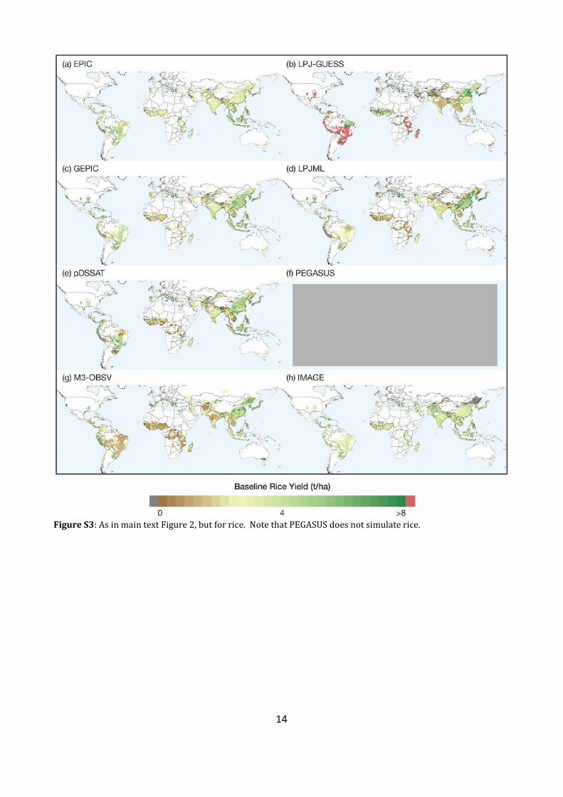
S3. Additional Results and Recommended Guidelines for Future Work Average reference period (1980-2010) wheat, rice, and soy yields are presented in Figures S2-S4. Figure S5 displays globally-aggregated production changes with CO2 effects separated by areas that are currently rainfed and areas with irrigation. Differences in production changes between rainfed and irrigated areas in any given model are generally smaller than the differences between simulations with and without CO2 effects. S3.1 General recommendations for the use of GGCM ensemble results from Phase 1 The seven GGCMs that provided data to the AgMIP/ISI-MIP Phase 1 archive differ in model type, implemented mechanisms, model calibration, and implicit and explicit assumptions. These differences have strong implications for the use and interpretation of data in analyses and assessments. We here want to point out a few general caveats but request from any researcher using these data to carefully check the suitability of the data for the intended analysis. If in doubt, please contact the individual GGCM modelers. Most obviously, some of the models have been calibrated to national or grid cell yield observations. This implies that absolute yield data are closer to observations, but it does not indicate models’ skill to simulate observed yield levels. Similarly, some of the GGCMs may have been applied in specific regions more than in others and may thus have implicit assumptions that suit cropping systems in these regions better than in others. Even though some GGCMs do not capture current yield patterns well (e.g. because of lacking calibration) the simulated relative yield trends may constitute valuable information to some applications such as economic assessments, if superimposed on observed yield patterns.
12
Many aspects, such as sensitivity to weather extremes and year-to-year variability have not been tested in detail. Analyses on these aspects need to evaluate the models’ skill in these aspects first. The AgMIP/ISI-MIP publications of Phase 1 provide a good orientation on GGCMs’ performance relative to the total range of results, which should be considered in the interpretation of the data. GGCM differences in model types, processes, inputs, and procedures imply ways that the results should be used. Relative yield changes should be used rather than absolute yield values since models differ in their calibration procedures as well as fertility inputs. For reference period yields, it is advisable to use an observation set such as the M3 data (Monfreda et al., 2008) adjusted to represent future yields using relative yield change factors calculated from the GGCMs. Furthermore, multi-year averages of yield results should be used because for some models yields are reported according to the year containing the harvest date and some years may not have reported yields or may have two harvests. Great care should be used in interpreting regional (i.e., continental, sub-continental, national, and sub-national) results, since the objective of this study was to conduct a global-scale intercomparison, and regional input data, model settings, and results have not been vetted. (See for example the discussion of accumulation of uncertainties in Roudier et al. 2011). We recommend that detailed validation be done at national and sub-national scales as a first step to use of these results at finer-than-global scales. Work is continuing to attribute climate sensitivity differences to disparities in GGCM properties and configurations. S3.2 AgMIP GGCM Intercomparison Phase II In the second phase of the AgMIP GGCM intercomparison, we will conduct a rigorous validation study and design protocols that provide further information relevant to policymakers. The next phase may also include updated versions of the models described here as well as a broader range of global gridded crop models (such as DayCent, Del Grosso et al., 2001; GLAM, Challinor et al., 2004, and Osborne et al., 2013; MCWLA (Tao et al., 2009); Orchidee-Mil, Berg et al., 2013). For example, the GGCM intercomparison protocol could include simulations without nutrient limitation and with harmonized planting dates. Since economic growth is likely to spur greater fertilizer applications in current low-input regions and improve management, this would improve comparability across models and adaptation planning and may additionally be more informative than trying to match current yields in low-input regions.

13
Figure S2: As in main text Figure 2, but for wheat.
14
Figure S3: As in main text Figure 2, but for rice. Note that PEGASUS does not simulate rice.

15
Figure S4: As in main text Figure 2, but for soybean.

16
Figure S5: As in main text Figure 4, but with rainfed and irrigated areas separated with CO2 effects.

17
References from Supplementary Information 1. Williams, J.R. (1995) The EPIC. In: Singh, V.P. (Ed.). Computer Models of Watershed Hydrology. Water Resources
Publications. Littleton, CO. pp. 909–1000 (Chapter 25). 2. Izaurralde, R.C., et al. (2006) Simulating soil C dynamics with EPIC: Model description and testing against long-
term data. Ecological Modeling 192(3-4):362-384. 3. Williams, J.R., et al. (1990) EPIC-Erosion/Productivity Impact Calculator. United States Department of Agriculture
Agricultural Research Service. Technical Bulletin Number 1768. Springfield, VA. 4. Liu, J. and Williams, J and Zehnder, A.J.B. and Yang, H., (2007) GEPIC–modelling wheat yield and crop water
productivity with high resolution on a global scale, Agricultural Systems, 94 (2), pp. 478–493 5. Leemans, R. and A.M. Solomon (1993) Modeling the potential change in yield and distribution of the earth’s crops
under a warmed climate. Climate Research 3:79-96. 6. Bouwman A.F., T. Kram, T. Klein, and K. Goldewijk (Eds.). (2006) Integrated Modelling of Global Environmental
Change. An Overview of IMAGE 2.4. PBL Netherlands Environmental Assessment Agency, The Hague. 7. Bondeau, A., et al. (2007) Modelling the role of agriculture for the 20th century global terrestrial carbon balance.
Global Change Biology 13:679–706, doi:10.1111/j.1365-2486.2006.01305.x 8. Fader, M., et al. (2010), Virtual water content of temperate cereals and maize: Present and potential future patterns,
Journal of Hydrology, 384, 218-231. 9. Waha, K., et al. (2012) Climate-driven simulation of global crop sowing dates. Global Ecology and Biogeography
21:247-259. 10. Schaphoff, S., U. Heyder, S. Ostberg, D. Gerten, J. Heinke, and W. Lucht (2013) Contribution of permafrost soils to
the global carbon budget, Environmental Research Letters. in press. 11. Smith, B., et al. (2001) Representation of vegetation dynamics in the modelling of terrestrial ecosystems: comparing
two contrasting approaches within European climate space. Global Ecology and Biogeography 10:621-637 12. Lindeskog M., et al. (in review) Implications of accounting for land use in simulations of ecosystem services and
carbon cycling in Africa. (in review at Earth Systems Dynamics) 13. Elliott, J., M. Glotter, N. Best, D. Kelly, M. Wilde, and I. Foster (2013). The Parallel System for Integrating Impact
Models and Sectors (pSIMS). Accepted for publication in the Proceedings of the 2013 XSEDE Conference. 14. Jones, J.W., et al. (2003) The DSSAT cropping system model. Eur. J. Agron. 18:235-265. 15. Deryng, D., W.J. Sacks, C.C. Barford, N. Ramankutty (2011) Simulating the effects of climate and agricultural
management practices on global crop yield. Global Biogeochem. Cycles 25(2) (/doi/10.1002/gbc.v25.2/issuetoc).
16. Adam, M., van Bussel, L. G. J., Leffelaar, P. A., Van Keulen, H., and Ewert, F. (2011). Effects of modelling detail on simulated potential crop yields under a wide range of climatic conditions. Ecological Modelling, 222(1):131–143.
17. Batjes, N.H. (2006) ISRIC-WISE Derived Soil Properties on a 5 by 5 Arc-minutes Global Grid. ISRIC – World Soil Information, Wageningen, Netherlands. (Available at http://www.isric.org.)
18. Schaap, M.G., and W. Bouten (1996). Modeling water retention curves of sandy soils using neural networks. Water Resources Research, 32(10), 3033-3040.
19. van Genuchten, M.T., F. Kaveh, and W.B. Russell, W.B. (1988) Direct and indirect methods for estimating the hydraulic properties of unsaturated soils \ Land qualities in space and time : proceedings of a symposium Wageningen, the Netherlands, 22 - 26 August 1988.
20. Dobos, E. (2006) Albedo. In Encyclopedia of Soil Science, Second Edition (pp. 64-66). 21. USDA/NRCS (2012): Soil Survey Staff, Natural Resources Conservation Service, Soil Survey Geographic
(SSURGO) Database for [Survey Area, State]. Available online at http://soildatamart.nrcs.usda.gov. Accessed Feb 2012.
22. Wood, S.R. and F.J. Dent (1983) LECS : a land evaluation computer system methodology. Part of: Manual / Food and Agriculture Organization Nr. no. 5, version 1
23. FAO (1991) The Digitized Soil Map of the World (Release 1.0). Food and Agriculture Organization of the United Nations)
24. FAO/IIASA/ISRIC/ISSCAS/JRC(2012) Harmonized World Soil Database (version 1.2), FAO, Rome, Italy and IIASA, Laxenburg, Austria.
25. Cosby, B.J., G.M. Hornberger, R.B. Clapp, and T.R. Ginn, T. R. (1984) A statistical exploration of the relationships of soil moisture characteristics to the physical properties of soils. Water Resources Research, 20(6), 682-690.
26. Lawrence, D.M., and A.G. Slater (2008) Incorporating organic soil into a global climate model. Climate Dynamics, 30(2-3), 145-160.
27. Sacks, W.J., D. Deryng, J.A. Foley, and N. Ramankutty (2010) Crop planting dates: an analysis of global patterns. Global Ecology and Biogeography 19:607-620.
28. You, L., et al. (2000) Spatial Production Allocation Model (SPAM) 2000 Version 3 Release 1. http://MapSPAM.info. (Accessed Feb, 2012).
18
29. Monfreda, C., Ramankutty, N. & Foley, J. A. (2008) Farming the planet: 2. Geographic distribution of crop areas, yields, physiological types, and net primary production in the year 2000. GBC 22, 19.Monteith, J.L. 1965. Evaporation and environment. Symposia of the Society for Experimental Biology 19: 205–224. PMID 5321565.
30. Willmott, C. J., et al. (1985) Statistics for the evaluation and comparison of models, J. Geophys. Res., 90(C5), 8995–9005.
31. Folberth, C., R. Gaiser, K.C. Abbaspour, R. Schulin, H. Yang (2012) Regionalization of a large-scale crop growth model for sub-Saharan Africa: Model setup, evaluation, and estimation of maize yields. Agriculture Ecosystems & Environment 151:21-33.
32. Farquhar, G. D., S. Caemmerer, J.A. Berry (1980) A biochemical model of photosynthetic CO2 assimilation in leaves of C3 species. Planta 149.
33. Deryng, D., et al. (2013) Global opportunities for producing more crops per drop under rising atmospheric CO2. PNAS, submitted to this special issue.
34. Penman, H.L. (1948) Natural Evaporation from Open Water, Bare Soil and G5 Grass. Proc. Roy. Soc. London A(194), S. 120-145.
35. Monteith, J. (1965) Evaporation and environment. Symp. Soc. Exp. Biol. 19:205-234. 36. Priestley, C.H.B. and R.J. Taylor (1972) On the assessment of surface heat flux and evaporation using large-scale
parameters. Monthly Weather Review 100 (2): 81–82. Bibcode 1972MWRv..100...81P. doi:10.1175/1520-0493(1972)100<0081:OTAOSH>2.3.CO;2.
37. Hargreaves, G.H. and Z.A. Samani (1985) Reference crop evapotranspiration from temperature. Transactions of ASAE 1(2):96-99.
38. Baier, W. and G. W. Robertson (1965) Estimation of latent evaporation from simple weather observations. Can. J. Plant Sci. 45:276-284.
39. Portmann, F.T., S. Siebert, P. Doll (2010) MIRCA2000 – global monthly irrigated and rainfed crop areas around the year 2000: a new high-resolution data set for agricultural and hydrological modelling. Global Biogeochemical Cycles 24:GB1011.
40. Kimball, B.A. 2011. Lessons from FACE: CO2 effects and interactions with water, nitrogen, and temperature. In Hillel, D. and Rosenzweig, C. (Eds.). Handbook of Climate Change and Agroecosystems: Impacts, Adaptation, and Mitigation. ICP Series on Climate Change Impacts, Adaptation, and Mitigation Vol 1. Imperial College Press. London. pp. 87-107.
41. Potter, Philip, Navin Ramankutty, Elena M. Bennett, Simon D. Donner (2010) Characterizing the Spatial Patterns of Global Fertilizer Application and Manure Production. Earth Interact., 14, 1–22.
42. Lobell, D.B., K.G. Cassman, and C.B. Field (2009) Crop Yield Gaps: Their Importance, Magnitudes, and Causes. Annu. Rev. Environ. Resour. 2009. 34:179–204
43. Roudier, P., B. Sultan, P. Quirion, C. Baron, A. Alhassane, S.B. Traore, and B. Muller (2011) The impact of future climate change on West African crop yields: What does the recent literature say? Global Environmental Change 21:1073-1083.
44. Del Grosso, et al. (Eds.) (2001) Modeling Carbon and Nitrogen Dynamics for Soil Management. CRC Press, Boca Raton, Florida, pp. 303-332.
45. Challinor, A.J., T.R. Wheeler, P.Q. Craufurd, J.M. Slingo, and D.I.F. Grimes (2004) Design and optimisation of a large-area process-based model for annual crops. Agric. For. Meteorol. 124, 99–120.
46. Osborne, T., G. Rose, and T. Wheeler (2013): Variation in the global-scale impacts of climate change on crop productivity due to climate model uncertainty and adaptation. Agric. For. Meteorol. 170, 183-194. doi:10.1016/j.agrformet.2012.07.006
47. Tao, F., M. Yokozawa, and Z. Zhang (2009) Modelling the impacts of weather and climate variability on crop productivity over a large area: A new process-based model development, optimization, and uncertainties analysis. Agric. For. Meteorol. 149, 831–850
48. Berg, A., N. de Noblet-Ducoudré, N., B. Sultan, M Lengaigne, and M. Guimberteau (2013) Projections of climate change impacts on potential C4 crop productivity over tropical regions. Agric. For. Meteorol. 170, 89-102. doi:10.1016/j.agrformet.2011.12.003