Critical state plasticity, Part VI: Meso-scale finite element

simulation of strain localization in discrete granular materials

Ronaldo I. Borja∗†, Jose E. Andrade

Department of Civil and Environmental Engineering, Stanford University, Stanford, CA 94305, USA

Abstract

Development of accurate mathematical models of discrete granular material behavior requires

a fundamental understanding of deformation and strain localization phenomena. This paper

utilizes a meso-scale finite element modeling approach to obtain an accurate and thorough

capture of deformation and strain localization processes in discrete granular materials such

as sands. We employ critical state theory and implement an elastoplastic constitutive model

for granular materials, a variant of a model called “Nor-Sand,” allowing for non-associative

plastic flow and formulating it in the finite deformation regime. Unlike the previous versions

of critical state plasticity models presented in a series of “Cam-Clay” papers, the present

model contains an additional state parameter ψ that allows for a deviation or detachment of

the yield surface from the critical state line. Depending on the sign of this state parameter,

the model can reproduce plastic compaction as well as plastic dilation in either loose or dense

granular materials. Through numerical examples we demonstrate how a structured spatial

density variation affects the predicted strain localization patterns in dense sand specimens.

∗Corresponding author. E-mail: borja@stanford.edu (R. I. Borja).†Supported by U.S. National Science Foundation, Grant Nos. CMS-0201317 and CMS-0324674

1 Introduction

Development of accurate mathematical models of discrete granular material behavior requires

a fundamental understanding of the localization phenomena, such as the formation of shear

bands in dense sands. For this reason, much experimental work has been conducted to gain

a better understanding of the localization process in these materials [1–11]. The subject also

has spurred considerable interest in the theoretical and computational modeling fields [12–29].

It is important to recognize that the material response observed in the laboratory is a result

of many different micro-mechanical processes, such as mineral particle rolling and sliding in

granular soils, micro-cracking in brittle rocks, and mineral particle rotation and translation

in the cement matrix of soft rocks. Ideally, any localization model for geomaterials must rep-

resent all of these processes. However, current limitations of experimental and mathematical

modeling techniques in capturing the evolution in the micro-scale throughout testing have

inhibited the use of a micro-mechanical description of the localized deformation behavior.

To circumvent the problems associated with the micro-mechanical modeling approach, a

macro-mechanical approach is often used. For soils, this approach pertains to the specimen

being considered as a macro-scale element from which the material response may be inferred.

The underlying assumption is that the specimen is prepared uniformly and deformed homo-

geneously enough to allow extraction of the material response from the specimen response.

However, it is well known that each specimen is unique, and that two identically prepared

samples could exhibit different mechanical responses in the regime of instability even if they

had been subjected to the same initially homogeneous deformation field. This implies that

the size of a specimen is too large to accurately resolve the macro-scale field, and that it can

only capture the strain localization phenomena in a very approximate way.

In this paper, we adopt a more refined approach to investigating strain localization phe-

nomena based on a meso-scale description of the granular material behavior. As a matter of

terminology, the term “meso-scale” is used in this paper to refer to a scale larger than the

grain scale (particle-scale) but smaller than the element, or specimen, scale (macro-scale).

This approach is motivated primarily by the current advances in laboratory testing capabil-

2

Figure 1: Cross-section through a biaxial specimen of silica sand analyzed by X-ray computedtomography; white spot is a piece of gravel.

ities that allow accurate measurements of material imperfection in the specimens, such as

X-ray Computed Tomography (CT) and Digital Image Processing (DIP) in granular soils

[2–4, 7, 29]. For example, Figure 1 shows the result of a CT scan on a biaxial specimen of

pure silica sand having a mean grain diameter of 0.5 mm and prepared via air pluviation.

The gray level variations in the image indicate differences in the meso-scale local density, with

lighter colors indicating regions of higher density (the large white spot in the lower level of

the specimen is a piece of gravel). This advanced technology in laboratory testing, combined

with DIP to quantitatively transfer the CT results as input into a numerical model, enhances

an accurate meso-scale description of granular material behavior and motivates the develop-

ment of robust meso-scale modeling approaches for replicating the shear banding processes in

discrete granular materials.

The modeling approach pursued in this paper utilizes nonlinear continuum mechanics and

the finite element method, in combination with a constitutive model based on critical state

plasticity that captures both hardening and softening responses depending on the state of the

material at yield. The first plasticity model exhibiting such features that comes to mind is the

classical modified Cam-Clay [24, 30–36]. However, this model may not be robust enough to

reproduce the shear banding processes, particularly in sands, since it was originally developed

3

to reproduce the hardening response of soils on the “wet” side of the critical state line, and

not the dilative response on the “dry” side where this model poorly replicates the softening

behavior necessary to trigger strain localization. To model the strain localization process

more accurately, we use an alternative critical state formulation that contains an additional

constitutive variable, namely, the state parameter ψ [37–39]. This parameter determines

whether the state point lies below or above the critical state line, as well as enables a complete

“detachment” of the yield surface from this line. By “detachment” we mean that the initial

position of the critical state line and the state of stress alone do not determine the density of the

material. Instead, one needs to specify the spatial variation of void ratio (or specific volume)

in addition to the state parameters required by the classical Cam-Clay models. Through the

state parameter ψ we can now prescribe quantitatively any measured specimen imperfection

in the form of initial spatial density variation.

Specifically, we use classical plasticity theory along with a variant of “Nor-Sand” model

proposed by Jefferies [38] to describe the constitutive law at the meso-scale level. The main

difference between this and the classical Cam-Clay model lies in the description of the evolu-

tion of the plastic modulus. In classical Cam-Clay model the character of the plastic modulus

depends on the sign of the plastic volumetric strain increment (determined from the flow rule),

i.e., it is positive under compaction (hardening), negative under dilation (softening), and is

zero at critical state (perfect plasticity). In sandy soils this may not be an accurate representa-

tion of hardening/softening responses since a dense sand could exhibit an initially contractive

behavior, followed by a dilative behavior, when sheared. This important feature, called phase

transformation in the literature [40, 41], cannot be reproduced by classical Cam-Clay models.

In the present formulation the growth or collapse of the yield surface is determined by the

deviatoric component of the plastic strain increment and by the position of the stress point

relative to a so-called limit hardening dilatancy. Such description reproduces more accurately

the softening response on the “dry” side of the critical state line.

The theoretical and computational aspects of this paper include the mathematical analyses

of the thermodynamics of constitutive models characterized by elastoplastic coupling [42, 43].

4

We also describe the numerical implementation of the finite deformation version of the model,

the impact of B-bar integration near the critical state, and the localization of deformation on

the “dry” side of the critical state line. We present two numerical examples demonstrating

the localization of deformation in plane strain and full 3D loading conditions, highlighting

in both cases the important role that the spatial density variation plays on the mechanical

responses of dense granular materials.

Notations and symbols used in this paper are as follows: bold-faced letters denote tensors

and vectors; the symbol ‘·’ denotes an inner product of two vectors (e.g. a · b = aibi), or a

single contraction of adjacent indices of two tensors (e.g. c ·d = cijdjk); the symbol ‘:’ denotes

an inner product of two second-order tensors (e.g. c : d = cijdij), or a double contraction of

adjacent indices of tensors of rank two and higher (e.g. C : ǫe = Cijklǫekl); the symbol ‘⊗’

denotes a juxtaposition, e.g., (a⊗b)ij = aibj . Finally, for any symmetric second order tensors

α and β,(α ⊗ β)ijkl = αijβkl, (α ⊕ β)ijkl = αjlβik, and (α ⊖ β)ijkl = αilβjk.

2 Formulation of the infinitesimal model

We begin by presenting the general features of the meso-scale constitutive model in the in-

finitesimal regime. Extension of the features to the finite deformation regime is then presented

in the next section.

2.1 Hyperelastic response

We consider a stored energy density function Ψ e(ǫe) in a granular assembly taken as a con-

tinuum; the macroscopic stress σ is given by

σ =∂Ψ e

∂ǫe(2.1)

where

Ψ e = Ψ e(ǫev) +

µeǫe 2

s (2.2)

5

and

Ψ(ǫev) = −p0κ exp ω , ω = −ǫev − ǫev0

κ, µe = µ0 +

α0

κΨ(ǫev). (2.3)

The independent variables are the infinitesimal macroscopic volumetric and deviatoric strain

invariants

ǫev = tr(ǫe) , ǫes =

√2

3‖ee‖ , ee = ǫe −

1

3ǫev1, (2.4)

where ǫe is the elastic component of the infinitesimal macroscopic strain tensor. The material

parameters required for definition are the reference strain ǫev0 and reference pressure p0 of the

elastic compression curve, as well as the elastic compressibility index κ. The above model

produces pressure-dependent elastic bulk and shear moduli, in accord with a well-known soil

behavioral feature. Equation (2.3) results in a constant elastic shear modulusµe = µ0 when

α0 = 0. This model is conservative in the sense that no energy is generated or lost in a closed

elastic loading loop [44].

2.2 Yield surface, plastic potential function, and flow rule

We consider the first two stress invariants

p =1

3trσ, q =

√3

2‖s‖, s = σ − p1, (2.5)

where p ≤ 0 in general. We define a yield function F of the form

F = q + ηp, (2.6)

where

η =

M [1 + ln (pi/p)] if N = 0;

M/N[1 − (1 −N) (p/pi)

N/(1−N)]

if N > 0.(2.7)

6

Here, pi < 0 is called the “image stress” representing the size of the yield surface, defined

such that the stress ratio η = −q/p = M when p = pi. A closed-form expression for pi is

pi

p=

exp(η/M − 1) if N = 0;

[(1 −N)/(1 − ηN/M)] if N > 0.(2.8)

The parameterN ≥ 0 determines the curvature of the yield surface on the hydrostatic axis and

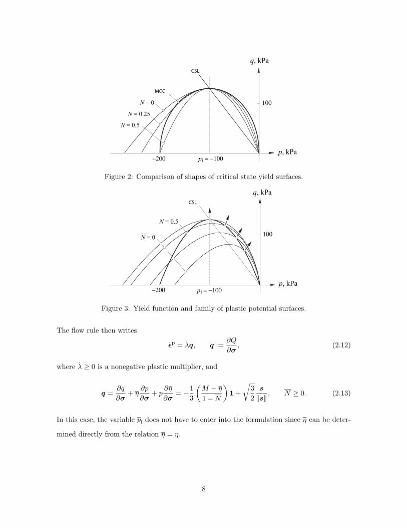
typically has a value less than 0.4 for sands [38]; asN increases, the curvature increases. Figure

2 shows yield surfaces for different values of N . For comparison, a plot of the conventional

elliptical yield surface used in modified Cam-Clay plasticity theory is also shown [30].

Next we consider a plastic potential function of the form

Q = q + ηp, (2.9)

where

η =

M [1 + ln(pi/p)] if N = 0;

(M/N)[1 − (1 −N)(p/pi)

N/(1−N)]

if N > 0.(2.10)

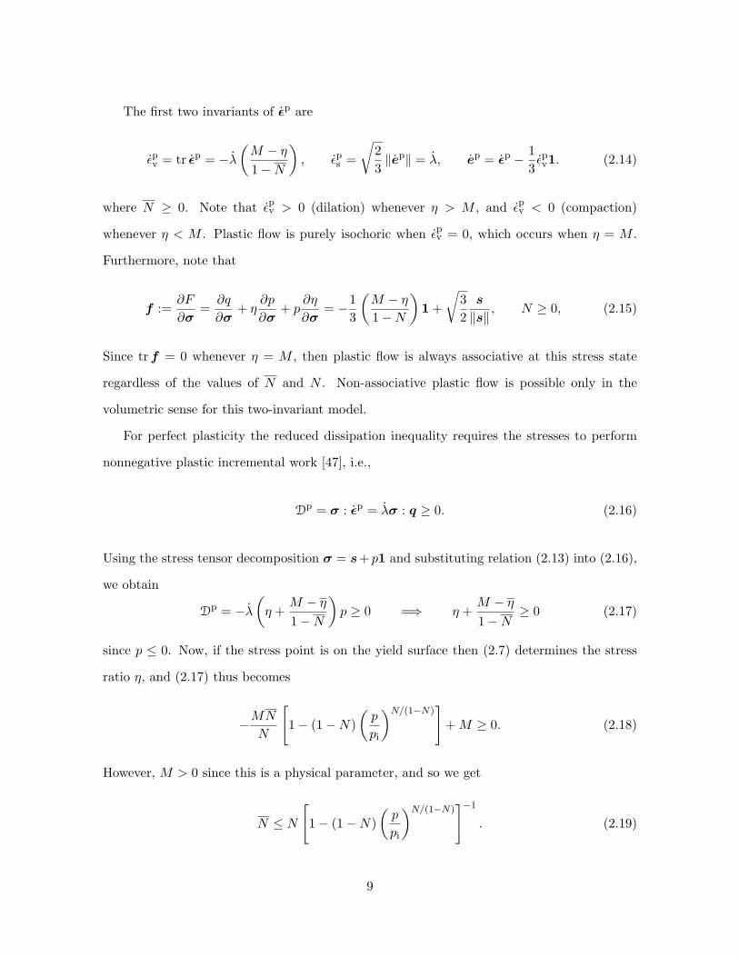
The plastic flow is associative if N = N and pi = pi, and non-associative otherwise. For the

latter case, we assume that N ≤ N resulting in a plastic potential function that is ‘flatter’

than the yield surface (if N < N), as shown in Figure 3. This effectively yields a smaller

dilatancy angle than is predicted by the assumption of associative normality, similar in idea to

the thermodynamic restriction that the dilatancy angle must be at most equal to the friction

angle in Mohr-Coulomb or Drucker-Prager materials, see [45, 46] for further elaboration.

The variable pi is a free parameter that determines the final size of the plastic potential

function. If we set Q = 0 whenever the stress point (p, q) lies on the yield surface, then pi can

be determined as

pi

p=

exp(η/M − 1) if N = 0;[(1 −N)/(1 − ηN/M)

](1−N)/Nif N > 0.

(2.11)

7

N = 0

N = 0.25

N = 0.5

MCC

q, kPa

p, kPa−200 p = −100i

CSL

100

Figure 2: Comparison of shapes of critical state yield surfaces.

N = 0.5

q, kPa

p, kPa−200 p = −100i

CSL

100N = 0

Figure 3: Yield function and family of plastic potential surfaces.

The flow rule then writes

ǫp = λq, q :=∂Q

∂σ, (2.12)

where λ ≥ 0 is a nonegative plastic multiplier, and

q =∂q

∂σ+ η

∂p

∂σ+ p

∂η

∂σ= −

1

3

(M − η

1 −N

)1 +

√3

2

s

‖s‖, N ≥ 0. (2.13)

In this case, the variable pi does not have to enter into the formulation since η can be deter-

mined directly from the relation η = η.

8

The first two invariants of ǫp are

ǫpv = tr ǫp = −λ

(M − η

1 −N

), ǫps =

√2

3‖ep‖ = λ, ep = ǫp −

1

3ǫpv1. (2.14)

where N ≥ 0. Note that ǫpv > 0 (dilation) whenever η > M , and ǫpv < 0 (compaction)

whenever η < M . Plastic flow is purely isochoric when ǫpv = 0, which occurs when η = M .

Furthermore, note that

f :=∂F

∂σ=∂q

∂σ+ η

∂p

∂σ+ p

∂η

∂σ= −

1

3

(M − η

1 −N

)1 +

√3

2

s

‖s‖, N ≥ 0, (2.15)

Since trf = 0 whenever η = M , then plastic flow is always associative at this stress state

regardless of the values of N and N . Non-associative plastic flow is possible only in the

volumetric sense for this two-invariant model.

For perfect plasticity the reduced dissipation inequality requires the stresses to perform

nonnegative plastic incremental work [47], i.e.,

Dp = σ : ǫp = λσ : q ≥ 0. (2.16)

Using the stress tensor decomposition σ = s+ p1 and substituting relation (2.13) into (2.16),

we obtain

Dp = −λ

(η +

M − η

1 −N

)p ≥ 0 =⇒ η +

M − η

1 −N≥ 0 (2.17)

since p ≤ 0. Now, if the stress point is on the yield surface then (2.7) determines the stress

ratio η, and (2.17) thus becomes

−MN

N

[1 − (1 −N)

(p

pi

)N/(1−N)]

+M ≥ 0. (2.18)

However, M > 0 since this is a physical parameter, and so we get

N ≤ N

[1 − (1 −N)

(p

pi

)N/(1−N)]−1

. (2.19)

9

The expression inside the pair of brackets is equal to unity at the stress space origin when

p = 0, reduces to N at the image stress point when η = M and p = pi, and is zero on the

hydrostatic axis when η = 0 and p = pi/(1−N)(1−N)/N . The corresponding inverses are equal

to unity, 1/N > 1, and positive infinity, respectively. Hence, for (2.19) to remain true at all

times, we must have

N ≤ N , (2.20)

as postulated earlier.

2.3 State parameter and plastic dilatancy

In classical Cam-Clay models the image stress pi coincides with a point on the critical state

line (CSL), a locus of points characterized by isochoric plastic flow in the space defined by

the stress invariants p and q and by the specific volume v. The CSL is given by the pair of

equations

qc = −Mpc, vc = vc0 − λ ln(−pc), (2.21)

where subscript “c” denotes that the point (vc, pc, qc) is on the CSL. The parameters are the

compressibility index λ and the reference specific volume vc0. Thus, any given point on the

yield surface has an associated specific volume, and isochoric plastic flow can only take place

on the CSL.

To apply the model to sands, which exhibit different types of volumetric yielding depending

on initial density, the yield surface is detached from the critical state line along the v-axis.

Thus, the state point (v, p, q) may now lie either above or below the critical specific volume vc

at the same stress p depending on whether the sand is looser or denser than critical. Following

the notations of [38], a state parameter ψ is introduced to denote the relative distance along

the v-axis of the current state point to a point vc on the CSL at the same p,

ψ = v − vc. (2.22)

Further, a state parameter ψi is introduced denoting the distance of the same current state

10

ln(− p)

v

− p

λ~

ψ < 0

− p i

ψi

CSL

v1

v2

vc

Figure 4: Geometric representation of state parameter ψ.

point to vc,i on the CSL at p = pi,

ψi = v − vc,i, vc,i = vc0 − λ ln(−pi), (2.23)

where vc,i is the value of vc at the stress pi, and vc0 is the reference value of vc when pi = 1,

see (2.21). The relation between ψ and ψi is (see Figure 4)

ψi = ψ + λ ln

(pi

p

). (2.24)

Hence, ψ is negative below the CSL and positive above it. An upshot of disconnecting the

yield surface from the CSL is that it is no longer possible to locate a state point on the

yield surface by prescribing p and q alone; one also needs to specify the state parameter

ψ to completely describe the state of a point. Furthermore, isochoric plastic flow does not

anymore occur only on the CSL but could also take place at the image stress point. Finally,

the parameter ψi dictates the amount of plastic dilatancy in the case of dense sands.

Formally, plastic dilatancy is defined by the expression

D := ǫpv/ǫps =

η −M

1 −N. (2.25)

11

This definition is valid for all possible values of η, even for η = 0 where Q is not a smooth

function. However, experimental evidence on a variety of sands suggests that there exists a

maximum possible plastic dilatancy, D∗, which limits a plastic hardening response. The value

of D∗ depends on the state parameter ψi, increasing in value as the state point lies farther and

farther away from the CSL on the dense side. An empirical correlation has been established

experimentally in [38] between the plastic dilatancy D∗ and the state parameter ψi, and takes

the form

D∗ = αψi, (2.26)

where α ≈ −3.5 typically for most sands. The corresponding value of stress ratio at this limit

hardening dilatancy is

η∗ = M +D∗(1 −N) = M + αψi(1 −N) = M + αψi(1 −N), (2.27)

and the corresponding size of the yield surface is

p∗ip

=

exp(αψi/M) if N = N = 0;

(1 − αψiN/M)(N−1)/N if 0 ≤ N ≤ N 6= 0,(2.28)

where

αβ = α, β =1 −N

1 −N. (2.29)

In the above expression we have introduced a non-associativity parameter β ≤ 1, where β = 1

in the associative case.

2.4 Consistency condition and hardening law

For elastoplastic response the standard consistency condition on the yield function F reads

F = f : σ −Hλ = 0 , λ > 0, (2.30)

12

where H is the plastic modulus given by the equation

H = −1

λ

∂F

∂pipi = −

1

λ

(p

pi

)1/(1−N)

Mpi. (2.31)

Since p/pi > 0, the sign of the plastic modulus depends on the sign of pi: H > 0 if pi < 0

(hardening), H < 0 if pi > 0 (softening), and H = 0 if pi = 0 (perfect plasticity).

In classical Cam-Clay theory the sign of H depends on the sign of ǫpv, i.e., H is positive

for compaction and negative for expansion. However, as noted above, this simple criterion

does not adequately capture the hardening/softening responses of sands, which are shown to

be dependent on the limit hardening plastic dilatancy D∗, i.e., H is positive if D < D∗ and

negative if D > D∗. Thus, any postulated hardening law must satisfy the obvious relationship

sgnH = sgn(−pi) = sgn(D∗ −D) = sgn(η∗ − η) = sgn(pi − p∗i ), (2.32)

where ‘sgn’ is the sign operator. Furthermore, in terms of the cumulative plastic shear strain

ǫps =

∫

tǫps dt, (2.33)

we require that

limǫps →∞

H = limǫps →∞

(−pi) = limǫps →∞

(D∗ −D) = limǫps →∞

(η∗ − η) = limǫps →∞

(pi − p∗i ) = 0. (2.34)

Thus, any postulated hardening law must reflect a condition of perfect plasticity as the plastic

shear strain becomes very large. Note that the above restriction is stronger, e.g., than the

weaker condition D∗ − D = 0, without the limit, which could occur even if the stress and

image points do not coincide. The limiting condition ǫps → ∞ insures that the stress and

image points approach the CSL, and that these two points coincide in the limit.

A general evolution for −pi satisfying the requirements stated above may be given by an

13

equation of the form

−pi = f(pi − p∗i )ǫps = f(pi − p∗i )λ, (2.35)

where f is a simple odd scalar function of its argument, i.e., f(−x) = −f(x) and sgn f = sgnx.

(Alternately, one can use either D or η in the argument for f). In this case, the expression

for the plastic modulus becomes

H = M

(p

pi

)1/(1−N)

f(pi − p∗i ). (2.36)

Taking f(x) = hx, where h is a positive dimensionless constant, we arrive at a phenomeno-

logical expression of the form similar to that presented in [38],

f(pi − p∗i ) = h(pi − p∗i ). (2.37)

This results in a plastic modulus given by the equation

H = Mh

(p

pi

)1/(1−N)

(pi − p∗i ). (2.38)

To summarize, the transition point between hardening and softening responses is represented

by the limit hardening dilatancy D∗, which approaches zero on the CSL.

2.5 Implications to entropy production

Consider the Helmholtz free energy function Ψ = Ψ(ǫe, ǫps ). For now, we avoid making the

usual additive decomposition of the free energy into Ψ = Ψ e(ǫe) + Ψp(ǫps ); in fact, we shall

demonstrate that such decomposition is not possible in the present model. Ignoring the

non-mechanical powers, the local Clausius-Duhem inequality yields

σ : ǫ −dΨ

dt≥ 0. (2.39)

14

Applying the chain rule for dΨ/dt and invoking the standard Coleman relations results in the

constitutive relation

σ =∂Ψ(ǫe, ǫps )

∂ǫe, (2.40)

plus the reduced dissipation inequality

σ : ǫp − piǫps ≥ 0 , pi =

∂Ψ(ǫe, ǫps )

∂ǫps. (2.41)

Here, we have chosen pi to be the stress-like plastic internal variable conjugate to ǫps . With an

appropriate set of material parameters we have ensured before that σ : ǫp ≥ 0 (see Sec. 2.2).

Since ǫps = λ ≥ 0 and pi < 0, the reduced dissipation inequality as written above holds

provided that

∂Ψ(ǫe, ǫps )

∂ǫps≤ 0. (2.42)

Now, consider the evolution for pi as postulated in (2.35). Integrating in time yields

∂Ψ(ǫe, ǫps )

∂ǫps≡ pi = pi0 −

∫ ǫps

ǫps0

f(pi − p∗i ) dǫps , (2.43)

where pi0 is the reference value of pi when ǫps = ǫps0. Recalling that f is a simple odd function,

the right-hand side of the above equation is negative provided that sgn(pi − p∗i ) = sgnH =

positive. This implies that the reduced dissipation inequality is identically satisfied in the

hardening regime.

Integrating once more gives a more definitive form of the Helmholtz free energy,

Ψ(ǫe, ǫps ) =

∫ ǫps

ǫps0

pi0 dǫps −

∫ ǫps

ǫps0

∫ ǫps

ǫps0

f(pi − p∗i ) dǫps dǫps + Ψ e(ǫe) + Ψ0, (2.44)

where Ψ e(ǫe) is the usual elastic stored energy function. The first two integrals represent the

plastic component of the free energy,

Ψp = Ψp(ǫe, ǫps ) =

∫ ǫps

ǫps0

pi0 dǫps −

∫ ǫps

ǫps0

∫ ǫps

ǫps0

f(pi − p∗i ) dǫps dǫps . (2.45)

15

Note in this case that Ψp depends not only on ǫps but also on ǫe through the variable p∗i . The

Cauchy stress tensor then becomes

σ =∂Ψ e(ǫe)

∂ǫe+

∫ ǫps

ǫps0

∫ ǫps

ǫps0

f ′(pi − p∗i )∂p∗i∂ǫe

dǫps dǫps

︸ ︷︷ ︸O(∆ǫp 2

s )

, (2.46)

where ∆ǫps = ǫps − ǫps0, and

∂p∗i∂ǫe

= (1 −N)αp∗i /M

1 − αψiN/M

∂ψi

∂ǫe+p∗ip

∂p

∂ǫe, N ≥ 0. (2.47)

Strictly, then, the Cauchy stress tensor depends not only on ǫe but also on ǫps . Attempts

have been made in the past to capture this dependence of σ on ǫps ; for example, a nonlinear

elasticity model in which the elastic shear modulus varies with a stress-like plastic internal

variable similar to pi has been proposed in [43, 48]. However, these developments have not

gained much acceptance in the literature due, primarily, to the lack of experimental data and

to the difficulty with obtaining such test data.

It must be noted that the observed dependence of Ψp on the elastic strain ǫe occurs only

prior to reaching the critical state where ∆ǫps remains “relatively small,” and thus, the second-

order term in (2.46) may be ignored (such as done in Sec. 2.1). Most of the intense shearing

(i.e., large ∆ǫps ) in fact occurs at the critical state where f(pi − p∗i ) = 0, at which condition

the additive decomposition of the free energy into Ψ e(ǫe) and Ψp(ǫps ) holds, see (2.44).

2.6 Numerical implementation

Even though the plastic internal variable pi depends on the state parameter ψi, and that this

variable is deeply embedded in the plastic modulus H, the model is still amenable to fully

implicit numerical integration. Table 1 summarizes the relevant rate equations used in the

constitutive theory. Table 2 summarizes the algorithmic counterpart utilizing the classical

return mapping scheme. For improved efficiency, the return mapping algorithm in Table 2

is performed in the strain invariant space, as demonstrated below, leading to a system of

16

Table 1: Summary of rate equations for plasticity model for sands, infinitesimal deformationversion.

1. Strain rates: ǫ = ǫe + ǫp

2. Hyperelastic rate equations: σ = ce : ǫe; c

e = ∂2Ψ e/∂ǫe∂ǫe

3. Flow rule: ǫp = λq

4. State parameter: ψi = v + λpi/pi from (2.23)

5. Hardening law: −pi = f(pi − p∗i )λ from (2.35)

6. Consistency condition: f : σ −Hλ = 0

7. Kuhn-Tucker conditions: λ ≥ 0, F ≤ 0, λF = 0

nonlinear equations with three unknowns. As usual, it is assumed that ∆ǫ is given, which

implies that both the elastic trial strain ǫe tr and the total strain ǫ are known. Note that v0

is the initial value of the specific volume at the beginning of the calculations when ǫ = 0,

and should not be confused with vc0. As usual, the main goal is to find the final stresses σ

and the discrete plastic multiplier ∆λ for a given strain increment ∆ǫ. Following [34, 45],

consider the following local residual equations generated by the applied strain increment ∆ǫ

r = r(x) =

ǫev − ǫe trv + ∆λβ∂pF

ǫes − ǫe trs + ∆λ∂qF

F

; x =

ǫev

ǫes

∆λ

(2.48)

where β is the non-associativity parameter defined in (2.29). The goal is to dissipate the

residual vector r by finding the solution vector x∗ using a local Newton iteration.

In developing the local Jacobian matrix r′(x) used for Newton iteration, it is convenient

to define the following mapping induced by the numerical algorithm

y =

p

q

pi

=

p(ǫev, ǫes)

q(ǫev, ǫes)

pi(ǫev, ǫ

es ,∆λ)

=⇒ y = y(x) (2.49)

17

Table 2: Return mapping algorithm for plasticity model for sands, infinitesimal deformationversion.

1. Elastic strain predictor: ǫe tr = ǫen + ∆ǫ

2. Elastic stress predictor: σtr = ∂Ψ e/∂ǫe tr ; ptri = pi,n

3. Check if yielding: F(σtr, ptr

i

)≥ 0?

No, set ǫe = ǫe tr; σ = σtr; pi = ptri and exit

4. Yes, initialize ∆λ = 0 and iterate for ∆λ (steps 5–7)

5. Plastic corrector: ǫe = ǫe tr − ∆λq, σ = ∂Ψ e/∂ǫe

6. Update plastic internal variable pi:

(a) Cumulative strain: ǫ = ǫn + ∆ǫ

(b) Specific volume: v = v0(1 + tr ǫ)

(c) Initialize pi = pi,n and iterate for pi (steps 6d-f)

(d) State parameter: ψi = v − vc0 + λ ln(−pi)

(e) Limit hardening plastic variable:

p∗i = p×

{exp (αψi/M) if N = N = 0,

(1 − αψiN/M)(N−1)/N if 0 ≤ N ≤ N 6= 0.

(f) Plastic internal variable: pi = pi,n − f(pi − p∗i )∆λ

7. Discrete consistency condition: F (p, q, pi) = 0

18

The tangent y′(x) = D defines the slope, given by

D =

D11 D12 D13

D21 D22 D23

D31 D32 D33

=

∂ǫevp ∂ǫesp 0

∂ǫevq ∂ǫesq 0

∂ǫevpi ∂ǫespi ∂∆λpi

. (2.50)

The hyperelastic equations take the following form independent of the discrete plastic multi-

plier ∆λ (and hence, D13 = D23 = 0)

p = p0 exp ω

[1 +

3α0

2κǫe 2s

], q = 3(µ0 − α0p0 expω)ǫes . (2.51)

Thus,

D11 = −p0

κexp ω

[1 +

3α0

2κǫe 2s

],

D22 = 3µ0 − 3α0p0 exp ω,

D12 = D21 =3p0α0ǫ

es

κexp ω. (2.52)

We recall that D21 = D12 from the postulated existence of an elastic stored energy function

Ψ e.

The plastic internal variable pi is deeply embedded in the evolution equations and is best

calculated iteratively, as shown in Table 2. First, from Step No. 6(f), we construct a scalar

residual equation

r(pi) = pi − pi,n + f(pi − p∗i )∆λ, (2.53)

where p∗i is calculated in succession from Step No. 6(e,d) of Table 2 using the current estimate

for pi. Using a sub-local Newton iteration, we determine the root that dissipates this residual

iteratively. The sub-local scalar tangent operator takes the simple form

r′(pi) = 1 + f ′(pi − p∗i )∆λ

[1 −

λα(1 −N)

M − αψiN

(p∗ipi

)], N ≥ 0. (2.54)

Having determined the converged value of pi, we can then calculate the corresponding values

19

of ψi and p∗i and proceed with the following differentiation.

From Table 2, Step No. 6(f), we obtain the variation

∂pi

∂ǫev= −f ′(pi − p∗i )∆λ

(∂pi

∂ǫev−∂p∗i∂ǫev

). (2.55)

From Step No. 6(e), we get

∂p∗i∂ǫev

=

(αp∗i

1 −N

M − αψiN

)∂ψi

∂ǫev+p∗ipD11, N ≥ 0. (2.56)

From Step No. 6(d), we obtain

∂ψi

∂ǫev=λ

pi

∂pi

∂ǫev. (2.57)

Combining these last three equations gives

D31 =∂pi

∂ǫev= c−1f ′(pi − p∗i )∆λ

(p∗ip

)D11;

c = 1 + f ′(pi − p∗i )∆λ

[1 −

λα(1 −N)

M − αψiN

(p∗ipi

)]. (2.58)

Note that c is the converged value of r′(pi) when r = 0, cf. (2.54). Following a similar

procedure, we obtain

D32 =∂pi

∂ǫes= c−1f ′(pi − p∗i )∆λ

(p∗ip

)D12. (2.59)

Again, using the same implicit differentiation, we get

D33 =∂pi

∂∆λ= −c−1f(pi − p∗i ). (2.60)

For the hardening law adopted in [38], f ′(pi − p∗i ) reduces to the constant h.

It is also convenient to define the following vector operator

H =

[H1 H2 H3

]=

[∂2

pp ∂2pq ∂2

ppi

]F . (2.61)

20

For the yield function at hand, the elements of H are as follows. First, we obtain the first

derivatives

∂F

∂p=

M ln(pi/p) if N = 0,

(M/N)[1 − (p/pi)N/(1−N)] if N > 0,

∂F

∂q= 1,

∂F

∂pi= M

(p

pi

)1/(1−N)

, N ≥ 0. (2.62)

Then, for N ≥ 0, we have

H1 = −1

1 −N

M

p

(p

pi

)N/(1−N)

, H2 = 0, H3 =1

1 −N

M

p

(p

pi

)1/(1−N)

. (2.63)

Finally, from the product formula induced by the chain rule, we define the vector operator G,

G = HD =

[G1 G2 G3

]. (2.64)

The algorithmic local tangent operator for Newton iteration is then given by

r′(x) = (2.65)

1 + ∆λβG1 ∆λβG2 β(∂pF + ∆λG3)

0 1 ∂qF

(D11∂p +D21∂q +D31∂pi)F (D12∂p +D22∂q +D32∂pi

)F D33∂piF

.

Remark 1. The numerical algorithm described above entails two levels of nested Newton

iterations to determine the local unknowns. An alternative approach would be to consider pi

as a fourth local unknown, along with ǫev, ǫes and ∆λ, and solve them all iteratively in one

single Newton loop. We have found that either approach works well for the problem at hand,

and that either one demonstrates about the same computational efficiency.

21

2.7 Algorithmic tangent operator

The algorithmic tangent operator c = ∂σ/∂ǫe tr ≡ ∂σ/∂ǫ is used for the global Newton

iteration of the finite element problem. It has been shown in [49, 50] that it can also be

used in lieu of the theoretically correct elastoplastic constitutive operator cep for detecting

the onset of material instability, provided the step size is ‘small.’ To derive the algorithmic

tangent operator, consider the following expression for the Cauchy stress tensor

σ = p1 +

√2

3qn, (2.66)

where n = s/‖s‖ = ee/‖ee‖ = ee tr/‖ee tr‖ from the co-axiality of the principal directions.

The chain rule then yields (see [34])

c =∂σ

∂ǫ= 1 ⊗

(D11

∂ǫev∂ǫ

+D12∂ǫes∂ǫ

)+

√2

3n ⊗

(D21

∂ǫev∂ǫ

+D22∂ǫes∂ǫ

)

+2q

3ǫe trs

(I −

1

31 ⊗ 1 − n ⊗ n

), (2.67)

where I is the fourth-rank identity tensor with components Iijkl = (δikδjl + δilδjk)/2. Our

goal is to obtain closed-form expressions for the derivatives ∂ǫev/∂ǫ and ∂ǫes/∂ǫ.

Using the same strain invariant formulation of the previous section, we now write the same

local residual vector as r = r(ǫe trv , ǫe tr

s ,x), where x is the vector of local unknowns. We recall

that the trial elastic strains were held fixed at the local level; however, at the global level they

themselves are now the iterates. Consequently, at the converged state where r = 0, we now

write the strain derivatives of the residual vector as

∂r

∂ǫ=∂r

∂ǫ

∣∣∣∣x

+

(∂r

∂x

∣∣∣∣ǫe trv ,ǫe tr

s

)·∂x

∂ǫ= 0, (2.68)

which gives

a ·∂x

∂ǫ= −

∂r

∂ǫ

∣∣∣∣x

=⇒∂x

∂ǫ= −b ·

∂r

∂ǫ

∣∣∣∣x

. (2.69)

We recognize a as the same 3 × 3 tangent matrix r′(x) in (2.65) evaluated at the locally

22

converged state, and b = a−1. In component form, we have

∂ǫev/∂ǫ

∂ǫes/∂ǫ

∂∆λ/∂ǫ

=

b11 b12 b13

b21 b22 b23

b31 b32 b33

=

(1 − ∆λβθH3)1√

2/3n

−θ∂piF1

, (2.70)

in which ∂pi/∂ǫ = θ1, and

θ = c−1∆λf ′(pi − p∗i )v0p∗i

α(1 −N)

M − αψiN, (2.71)

is the linearization of the term associated with the state parameter ψi. This facilitates the

solution of the desired strain derivatives,

∂ǫev∂ǫ

= b111 +

√2

3b12n,

∂ǫes∂ǫ

= b211 +

√2

3b22n, (2.72)

where

b11 = (1 − ∆λβθH3)b11 − (θ∂piF )b13,

b21 = (1 − ∆λβθH3)b21 − (θ∂piF )b23. (2.73)

Defining the matrix product

D11 D12

D21 D22

=

D11 D12

D21 D22

b11 b12

b21 b22

, (2.74)

the consistent tangent operator then becomes

c =

(D11 −

2q

9ǫe trs

)1 ⊗ 1 +

√2

3

(D121 ⊗ n +D21n ⊗ 1

)

+2q

3ǫe trs

(I − n ⊗ n) +2

3D22n ⊗ n. (2.75)

In the elastic regime the submatrix [ bij ] becomes an identity matrix, and hence Dij = Dij

23

for i, j = 1, 2. In this case, c reduces to the hyperelastic tangent operator ce.

Remark 2. As shown in Figure 3, the proposed yield and plastic potential functions create

corners on the compaction side of the hydrostatic axis. While the model is primarily developed

to accurately capture dilative plastic flow, and therefore is not expected to perform well in

stress states dominated by hydrostatic compaction, numerical problems could still arise in

general boundary-value problem simulations when the stress ratio η as defined by (2.7) goes

to zero or even becomes negative. In order to avoid a negative η, we introduce a ‘cap’ on the

plastic potential function such that

Q =

q + ηp if η = η ≥ χM ,

−p if η = η < χM ,(2.76)

where χ is a user-specified parameter controlling the position of the plastic potential function

cap, e.g., χ = 0.10. For the case where η < χM , the local residual vector simplifies to

r(x) =

ǫev − ǫe trv − ∆λ

ǫes − ǫe trs

F

. (2.77)

The local tangent operator is given by

r′(x) =

1 0 −1

0 1 0

(D11∂p +D21∂q)F (D12∂p +D22∂q)F 0

. (2.78)

Finally, the strain derivative of r holding x fixed reduces to

∂r

∂ǫ

∣∣∣∣x

=

1

√2/3n

0

. (2.79)

Of course, one can also insert a smooth cap near the nose of the plastic potential function as

24

an alternative to the planar cap.

3 Finite deformation plasticity; localization of deformation

In the preceding section we have reformulated an infinitesimal rigid-plastic constitutive model

for sands to accommodate non-associated plasticity and hyperelasticity. In this section we

further generalize the model to accommodate finite deformation plasticity. The final model is

then used to capture deformation and failure initiation in dense sands, focusing on the effects

of uneven void distribution on the local and global responses.

3.1 Entropy inequality

Consider the multiplicative decomposition of deformation gradient for a local material point

X [51–53]

F (X, t) = F e(X, t) · F p(X, t). (3.1)

In the following we shall use as a measure of elastic deformation the contravariant tensor field

be reckoned with respect to the current placement, called the left Cauchy-Green deformation

tensor,

be = F e · F e t. (3.2)

Assume then that the free energy is given by

Ψ = Ψ(X, be, εps ). (3.3)

As in the infinitesimal model, we investigate conditions under which we could isolate an elastic

stored energy function from the above free energy function.

For the purely mechanical theory the local dissipation function takes the form

D = τ : d −dΨ(X, be, εps )

dt≥ 0, (3.4)

where τ = Jσ is the symmetric Kirchhoff stress tensor, J = det(F ), d = sym(l) is the rate of

25

deformation tensor, and l is the spatial velocity gradient. Using the chain rule and invoking

the standard Coleman relations yields the constitutive equation [54]

τ = 2∂Ψ(X, be, εps )

∂be · be, (3.5)

along with the reduced dissipation inequality

D = τ : dp − πiεps ≥ 0, (3.6)

where dp is the plastic component of the rate of deformation,

dp = sym(lp), lp := F e · Lp · F e−1, Lp := Fp· F p−1, (3.7)

and

πi =∂Ψ(X, be, εps )

∂εps, (3.8)

is a stress-like plastic internal variable equivalent to pi of the infinitesimal theory.

We assume that πi evolves in the same way as pi, i.e.,

−πi = φ(πi − π∗i )εps , (3.9)

where π∗i depends not only on πi but also on be. Integrating (3.9) gives

πi = πi0 −

∫ εps

εps0

φ(πi − π∗i ) dεps . (3.10)

Integrating once more, we get

Ψ(X, be, εps ) =

∫ εps

εps0

πi0 dεps −

∫ εps

εps0

∫ εps

εps0

φ(πi − π∗i ) dεps dεps + Ψ e(X, be) + Ψ0, (3.11)

where Ψ e(X, be) is the elastic stored energy function. Finally, using the constitutive equation

26

(3.5) once again, we get

τ = 2

∂Ψ e(X, be)

∂be +

∫ εps

εps0

∫ εps

εps0

φ′(πi − π∗i )∂π∗i∂be dεps dε

ps

︸ ︷︷ ︸O(∆εp

s2)

· be. (3.12)

The second-order terms in (3.12) can be ignored at the initial stage of loading when ∆εps is

small, thus leaving the Kirchhoff stress varying with the elastic stored energy function alone.

When ∆εps is large, φ(πi −π∗i ) vanishes at critical state, and so the elastic and plastic parts of

the free energy uncouple. In both cases the stresses can be expressed in terms of the elastic

stored energy function alone, i.e.,

τ = 2∂Ψ e(X, be)

∂be · be. (3.13)

Once again, the perfectly plastic behavior at critical state is a key feature of the model that

allows for the uncoupling of the free energy.

3.2 Finite deformation plasticity model

Consider the stress invariants

p =1

3tr τ , q =

√3

2‖ξ‖, ξ = τ − p1. (3.14)

Then, as in the infinitesimal theory the yield function can be defined as

F = q + ηp ≤ 0, (3.15)

where

η =

M [1 + ln(πi/p)] if N = 0;

(M/N)[1 − (1 −N)(p/πi)

N/(1−N)]

if N > 0.(3.16)

27

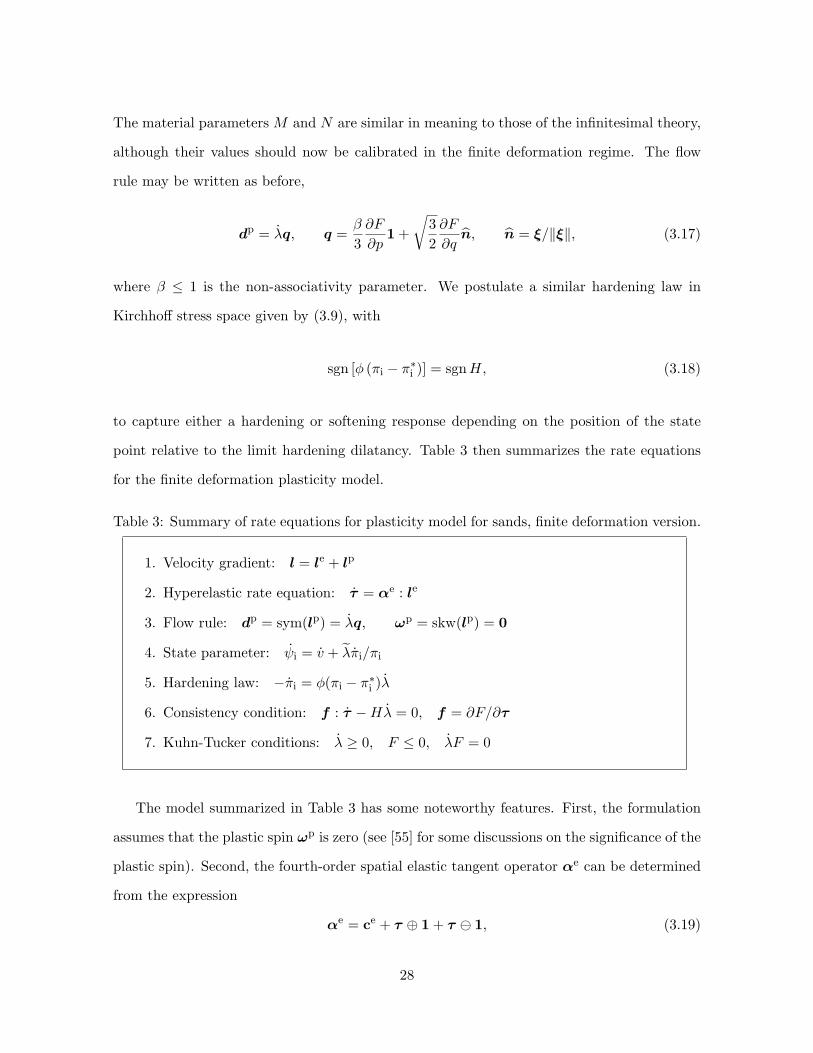
The material parameters M and N are similar in meaning to those of the infinitesimal theory,

although their values should now be calibrated in the finite deformation regime. The flow

rule may be written as before,

dp = λq, q =β

3

∂F

∂p1 +

√3

2

∂F

∂qn, n = ξ/‖ξ‖, (3.17)

where β ≤ 1 is the non-associativity parameter. We postulate a similar hardening law in

Kirchhoff stress space given by (3.9), with

sgn [φ (πi − π∗i )] = sgnH, (3.18)

to capture either a hardening or softening response depending on the position of the state

point relative to the limit hardening dilatancy. Table 3 then summarizes the rate equations

for the finite deformation plasticity model.

Table 3: Summary of rate equations for plasticity model for sands, finite deformation version.

1. Velocity gradient: l = le + lp

2. Hyperelastic rate equation: τ = αe : le

3. Flow rule: dp = sym(lp) = λq, ωp = skw(lp) = 0

4. State parameter: ψi = v + λπi/πi

5. Hardening law: −πi = φ(πi − π∗i )λ

6. Consistency condition: f : τ −Hλ = 0, f = ∂F/∂τ

7. Kuhn-Tucker conditions: λ ≥ 0, F ≤ 0, λF = 0

The model summarized in Table 3 has some noteworthy features. First, the formulation

assumes that the plastic spin ωp is zero (see [55] for some discussions on the significance of the

plastic spin). Second, the fourth-order spatial elastic tangent operator αe can be determined

from the expression

αe = ce + τ ⊕ 1 + τ ⊖ 1, (3.19)

28

where (τ ⊕ 1)ijkl = τjlδik, (τ ⊖ 1)ijkl = τilδjk, and ce is a spatial tangential elasticity tensor

obtained from the push-forward of all the indices of the second tangential elasticity tensor

defined in [52]. Finally, the specific volume varies according to the kinematical relation

v = Jv0 =⇒ v = Jv0 = Jv0 tr(l) = v tr(l). (3.20)

Thus, just as in the infinitesimal theory where the rate equations may be viewed as driven by

the strain rate ǫ, the rate equations shown in Table 3 may be viewed as driven by the spatial

velocity gradient l.

3.3 Numerical implementation

For the problem at hand we employ a standard elastic predictor-plastic corrector algorithm

based on the product formula for be, as summarized in Table 4. Let

ben = F e

n · F e tn . (3.21)

Suppressing plastic flow, the trial elastic predictor for be is

be tr ≡ be trn+1 = fn+1 · b

en · f t

n+1 , fn+1 =∂xn+1

∂xn. (3.22)

The plastic corrector emanates from the exponential approximation

be = exp(−2∆λq) · be tr , q ≡ qn+1 =∂Q

∂τ. (3.23)

From the co-axiality of plastic flow, the principal directions of q and τ coincide.

Next we obtain a spectral decomposition of be,

be =3∑

A=1

(λeA)2m(A) , m(A) = n(A) ⊗ n(A), (3.24)

where λeA are the elastic principal stretches, n(A) are the unit principal directions, and m(A)

29

Table 4: Return mapping algorithm for plasticity model for sands, finite deformation version.

1. Elastic deformation predictor: be tr = fn+1 · ben · f t

n+1

2. Elastic stress predictor: τ tr = 2(∂Ψ e/∂be tr) · be tr; πtri = πi,n

3. Check if yielding: F (ptr, qtr, πtri ) ≥ 0?

No, set be = be tr; τ = τ tr; πi = πtri and exit

4. Yes, initialize ∆λ = 0 and iterate for ∆λ (steps 5-8)

5. Spectral decomposition: be tr =∑3

A=1(λe trA )2mtr(A)

6. Plastic corrector in principal logarithmic stretches: εeA = ln(λeA),

εe trA = ln(λe tr

A ), εeA = εe trA − ∆λqA, τA = ∂Ψ e/∂εeA , A = 1, 2, 3.

7. Update plastic internal variable πi:

(a) Total deformation gradient: F = fn+1 · F n

(b) Specific volume: v = v0 detF = v0J

(c) Initialize πi = πi,n and iterate for πi (steps 7d-f)

(d) State parameter: ψi = v − vc0 + λ ln (−πi)

(e) Limit hardening plastic variable:

π∗i = p×

{exp (αψi/M) if N = N = 0,

(1 − αψiN/M)(N−1)/N if 0 ≤ N ≤ N 6= 0.

(f) Plastic internal variable: πi = πi,n − φ(πi − π∗i )∆λ

8. Discrete consistency condition: F (p, q, πi) = 0

9. Spectral resolution: be =∑3

A=1(λeA)2mtr(A)

30

are the spectral directions. The corresponding elastic logarithmic stretches are

εeA = ln(λeA) , A = 1, 2, 3. (3.25)

From material frame indifference Ψ e(X, be) only varies with εeA, and so we can write Ψ e =

Ψ e(X, εe1, εe2, ε

e2), which gives

∂Ψ e

∂be =1

2

3∑

A=1

1

(λeA)2

∂Ψ e

∂εeAm(A). (3.26)

The elastic constitutive equation then writes

τ = 2∂Ψ e

∂be · be =3∑

A=1

τAm(A) , τA =∂Ψ e

∂εeA, (3.27)

implying that the spectral directions of τ and be also coincide. Thus, be and q are also

co-axial, and for (3.23) to hold, be and be tr must also be co-axial, i.e.,

m(A) = mtr (A). (3.28)

This allows the plastic corrector phase to take place along the principal axes, as shown in

Table 4.

Alternatively, we can utilize the algorithm developed for the infinitesimal theory by work-

ing on the invariant space of the logarithmic elastic stretch tensor. Let

εev = εe1 + εe2 + εe3 , εes =1

3

√2[(εe1 − εe2)

2 + (εe1 − εe3)2 + (εe2 − εe3)

2], (3.29)

denote the first two invariants of the logarithmic elastic stretch tensor (similar definitions may

be made for εe trv and εe tr

s ), and

p =1

3(τ1 + τ2 + τ3) , q =

√[(τ1 − τ2)2 + (τ1 − τ3)2 + (τ2 − τ3)2]/2, (3.30)

31

denote the first two invariants of the Kirchhoff stress tensor. If we take the functional re-

lationships p = p(εev, εes), q = q(εev, ε

es), and πi = πi(ε

ev, ε

es ,∆λ) as before, using the same

elastic stored energy function but now expressed in terms of the logarithmic principal elastic

stretches, then the local residual vector writes

r = r(x) =

εev − εe trv + ∆λβ∂pF

εes − εe trs + ∆λ∂qF

F

; x =

εev

εes

∆λ

. (3.31)

In this case, the local Jacobian r′(x) takes a form identical to that developed for the infinites-

imal theory, see (2.65).

Comparing Tables 2 and 4, we see that the algorithm for finite deformation plasticity

differs from the infinitesimal version only through a few additional steps entailed for the

spectral decomposition and resolution of the deformation and stress tensors. Construction of

be from the spectral values requires two steps. The first involves resolution of the principal

elastic logarithmic stretches from the first two invariants calculated from return mapping,

εeA =1

3εevδA +

√3

2εesnA , nA =

√2

3

εe trA − (εe tr

v /3)δAεe trs

, (3.32)

where δA = 1 for A = 1, 2, 3.The above transformation entails scaling the deviatoric com-

ponent of the predictor tensor by the factor εes/εe trs and adding the volumetric component.

The second step involves a spectral resolution from the principal elastic logarithmic strains

(cf. (3.24))

be =3∑

A=1

exp(2εeA)mtr (A). (3.33)

The next section demonstrates that a closed-form consistent tangent operator is available for

the above algorithm.

32

3.4 Algorithmic tangent operator

For simplicity, we restrict to a quasi-static problem whose weak form of the linear momentum

balance over an initial volume B with surface ∂B reads

∫

B

(GRAD η : P − ρ0η · G) dV −

∫

∂Bt

η · t dA = 0, (3.34)

where ρ0G is the reference body force vector, t = P · n is the nominal traction vector on

∂Bt ⊂ ∂B, n is the unit vector on ∂Bt, η is the weighting function,

P = τ · F−t (3.35)

is the nonsymmetric first Piola-Kirchhoff stress tensor, and GRAD is the gradient operator

evaluated with respect to the reference configuration. We recall the internal virtual work

W eINT =

∫

Be

GRADη : P dV =

∫

Be

gradη : τ dV (3.36)

for any Be ⊂ B, where grad is the gradient operator evaluated with respect to the current

configuration. The first variation gives [56]

δW eINT =

∫

Be

gradη : a : grad δudV , (3.37)

where u is the displacement field, and

a = α − τ ⊖ 1, δτ = α : grad δu. (3.38)

Evaluation of a thus requires determination of the algorithmic tangent operator α.

We also recall the following spectral representation of the algorithmic tangent operator α

33

[56]

α =3∑

A=1

3∑

B=1

aABm(A) ⊗ m(B) (3.39)

+3∑

A=1

∑

B 6=A

τB − τAλe tr 2

B − λe tr 2A

(λe tr 2

B m(AB) ⊗ m(AB) + λe tr 2A m(AB) ⊗ m(BA)

),

where m(AB) = n(A) ⊗ n(B), A 6= B. The coefficients aAB are elements of the consistent

tangent operator obtained from a return mapping in principal axes, and is formally defined

as

aAB =∂τA∂εe tr

B

≡∂τA∂εB

, A,B = 1, 2, 3. (3.40)

The values of these coefficients are specific to the constitutive model in question, as well as

dependent on the numerical integration algorithm utilized for the model. For the present

critical state plasticity theory aAB is evaluated as follows.

The expression for a principal Kirchhoff stress is

τA = pδA +

√2

3q nA , A = 1, 2, 3. (3.41)

Differentiating with respect to a principal logarithmic strain gives

aAB =∂τA∂εB

= δA

(D11

∂εev∂εB

+D12∂εes∂εB

)+

√2

3nA

(D21

∂εev∂εB

+D22∂εes∂εB

)

+2q

3εe trs

(δAB −

1

3δAδB − nAnB

), A,B = 1, 2, 3, (3.42)

where δAB is the Kronecker delta. The coefficients D11, D22, and D21 are identical in form to

those shown in (2.52) except that the strain invariants now take on logarithmic definitions.

As in the infinitesimal theory, we obtain the unknown strain derivatives above from the local

residual vector, whose own derivatives write

∂rA∂εB

=∂rA∂εB

∣∣∣∣x

+3∑

C=1

∂rA∂xC

∣∣∣∣εe trv ,εe tr

s︸ ︷︷ ︸aAC

∂xC

∂εB= 0, A,B = 1, 2, 3, (3.43)

34

where the matrix [aAB] corresponds to the same algorithmic local tangent operator given in

(2.65). Letting [bAB] denote the inverse of [aAB], we can then solve

∂xA

∂εB= −

3∑

C=1

bAC∂rC∂εB

∣∣∣∣x

, A,B = 1, 2, 3. (3.44)

This latter equation provides the desired strain derivatives,

∂εev/∂εA

∂εes/∂εA

∂∆λ/∂εA

=

b11 b12 b13

b21 b22 b23

b31 b32 b33

(1 − ∆λβθH3)δA√

2/3nA

−θ∂πiFδA

, A = 1, 2, 3, (3.45)

where

θ = c−1∆λφ′(πi − π∗i )vπ∗i

α(1 −N)

M − αψiN,

c = 1 + φ′(πi − π∗i )∆λ

[1 −

λα(1 −N)

M − αψiN

(π∗iπi

)]. (3.46)

Note that the finite deformation expression for θ utilizes the current value of the specific

volume v whereas the infinitesimal version uses the initial value v0 (cf. (2.71)). Inserting the

expressions for ∂εev/∂εA and ∂εes/∂εA back in (3.42) yields the closed-form solution for aAB,

which takes an identical form to (2.75):

aAB =

(D11 −

2q

9εe trs

)δAδB +

√2

3

(D12δAnB +D21nAδB

)

+2q

3εe trs

(δAB − nAnB) +2

3D22nAnB, A,B = 1, 2, 3. (3.47)

See (2.72)–(2.74) for specific expressions for the coefficients Dij .

3.5 Localization condition

Following [56, 57], we summarize the following alternative (and equivalent) expressions for the

localization condition into planar bands. We denote the continuum elastoplastic counterpart

35

of the algorithmic tensor α by

αep =3∑

A=1

3∑

B=1

aepABm(A) ⊗ m(B) (3.48)

+3∑

A=1

∑

B 6=A

τB − τAλe 2

B − λe 2A

(λe 2

B m(AB) ⊗ m(AB) + λe 2A m(AB) ⊗ m(BA)

),

where aepAB is the continuum elastoplastic tangent stiffness matrix in principal axes. (Note,

this formula appears in [45, 49, 50] with a factor “1/2” before the spin-term summations, a

typographical error). Then,

aep = αep − τ ⊖ 1 (3.49)

defines the continuum counterpart of the fourth-order tensor a in (3.38).

Alternatively, we denote the constitutive elastoplastic material tensor cep by the expression

[54]

cep =

3∑

A=1

3∑

B=1

aepABm(A) ⊗ m(B) +

3∑

A=1

τAω(A), (3.50)

in which

ω(A) = 2[Ib − be ⊗ be + I3b

−1A (1 ⊗ 1 − I) + bA(be ⊗ m(A) + m(A) ⊗ be)

− I3b−1A (1 ⊗ m(A) + m(A) ⊗ 1) + ψm(A) ⊗ m(A)

]/DA, (3.51)

where bA is the Ath principal value of be, I1 and I3 are the first and third invariants of be,

Ib = (be ⊕ be + be ⊖ be)/2, ψ = I1bA + I3b−1A − 4b2A, (3.52)

and

DA := 2b2A − I1bA + I3b−1A . (3.53)

Note that cepijkl = 2FiAFjBFkCFlDCep

ABCD is the spatial push-forward of the first tangential

36

elastoplastic tensor Cep [52]. Then,

aep = c

ep + τ ⊕ 1 (3.54)

defines an alternative expression to (3.49).

Using aep from either (3.49) or (3.54), we can evaluate the elements of the Eulerian

elastoplastic acoustic tensor a as

aij = nkaepikjlnl, (3.55)

where nk and nl are elements of the unit normal vector n to a potential deformation band

reckoned with respect to the current configuration. Defining the localization function as

F = inf∣∣n(det a), (3.56)

we can then infer the inception of a deformation band from the initial vanishing of F. Though

theoretically one needs to use the constitutive operators αep or cep to obtain the acoustic

tensor a, the algorithmic tangent tensors are equally acceptable for bifurcation analyses for

small step sizes [50].

4 Numerical simulations

We present two numerical examples demonstrating the meso-scale modeling technique. To

highlight the triggering of strain localization via imposed material inhomogeneity, we only

considered regular specimens (either rectangular or cubical) along with boundary conditions

favoring the development of homogeneous deformation (a pin to arrest rigid body modes

and vertical rollers at the top and bottom ends of the specimen). A common technique of

perturbing the initial condition is to prescribe a weak element; however, this is unrealistic and

arbitrary. In the following simulations we have perturbed the initial condition by prescribing

a spatially varying specific volume (or void ratio) consisting of horizontal layers of relatively

homogeneous density but with some variation in the vertical direction. This resulted in vein-

37

like soil structures in the density field closely resembling that shown in the photograph of

Figure 1 and mimicked the placement of sand with a common laboratory technique called

pluviation. The specific volume fields were assumed to range from 1.60 to 1.70, with a mean

value of 1.63. These values were chosen such that all points remained on the dense side of the

CSL (ψi < 0).

4.1 Plane strain simulation

As a first example we considered a finite element mesh 1 m wide and 2 m tall and consisting

of 4,096 constant strain triangular elements shown in Figure 5. The mesh is completely

symmetric to avoid any bias introduced by the triangles. The vertical sides were subjected to

pressure loads (natural boundary condition), whereas the top end was compressed by moving

roller supports (essential boundary condition). The load-time functions are shown in Figure

6 with scaling factors γ = 100 kPa and β = 0.40 m for pressure load G1(t) and vertical

compression G2(t), respectively. The material parameters are summarized in Tables 5 and

6 and roughly represent those of dense Erksak sand, see [38]. The preconsolidation stress

was set to pc = −130 kPa and the reference specific volume was assumed to have a value

vc0 = 1.915 (uniform for all elements). The distribution of initial specific volume is shown in

Figure 7.

38

( )= ( )F t G tb 1

d t G t( )= ( )g 2

( )F t

d t( )

Figure 5: Finite element mesh for plane strain compression problem.

t0 0.2 0.4 0.6 0.8 1.0

0.2

0.4

0.6

0.8

1.0

G (t), G (t)1 2

G (t)1

0.0

G (t)2

Figure 6: Load-time functions.

39

Symbol Value Parameter

κ 0.03 compressibilityα0 0 coupling coefficientµ0 2000 kPa shear modulusp0 −100 kPa reference pressureǫev0 0 reference strain

Table 5: Summary of hyperelastic material parameters (see [44] for laboratory testing proce-dure).

Symbol Value Parameter

λ 0.04 compressibilityN 0.4 for yield function

N 0.2 for plastic potentialh 280 hardening coefficient

Table 6: Summary of plastic material parameters (see [38] for laboratory testing procedure).

Figure 8 shows contours of the determinant function and the logarithmic deviatoric strains

at the onset of localization for the case of finite deformations, which occurred at a nominal

axial strain of 12.26%. Localization for the infinitesimal model was slightly delayed at 12.34%.

The figure shows a clear correlation between regions in the specimen where the determinant

function vanished for the first time and where the deviatoric strains were most intense. Fur-

thermore, the figure reveals an X-pattern of shear band formation captured by both shear

deformation and determinant function contours, reproducing those observed in laboratory

experiments [1, 6].

40

1.61

1.62

1.63

1.64

1.65

1.66

1.67

1.68

1.69

Figure 7: Initial specific volume for plane strain compression problem.

0.5

1

1.5

2

2.5

x 107

0.12

0.13

0.14

0.15

0.16

0.17

0.18

(a) (b)

Figure 8: Contours of: (a) determinant function; and (b) deviatoric invariant of logarithmic

stretches at onset of localization.

Figure 9 displays contours of the plastic modulus and the logarithmic volumetric strains

at the onset of localization. We recall that for this plasticity model the plastic modulus is a

41

0.01

0.02

0.03

0.04

0.05

0.06

0.07

0.08

0.09

−0.05

−0.048

−0.046

−0.044

−0.042

−0.04

−0.038

−0.036

−0.034

(a) (b)

Figure 9: Contours of: (a) plastic hardening modulus; and (b) volumetric invariant of loga-rithmic stretches at onset of strain localization.

function of the state of stress, and in this figure low values of hardening modulus correlate

with areas of highly localized shear strains shown in Figure 8. On the other hand, volumetric

strains at localization appear to resemble the initial distribution of specific volume shown in

Figure 7. In fact the blue pocket of high compression extending horizontally at the top of

the sample (Figure 9b) is representative of that experienced by the red horizontal layer of

relatively low density shown in Figure 7. The calculated shear bands were predominantly

dilative.

4.2 Three-dimensional simulation

For the 3D simulation we considered a cubical finite element mesh shown in Figure 10. The

mesh is 1 m wide by 1 m deep by 2 m tall and consists of 2000 eight-node brick elements. All

four vertical faces of the mesh were subjected to pressure loads of 100 kPa (natural boundary

condition). The top face at z = 2 m was compressed vertically by moving roller supports

according to the same load-time function shown in Figure 6 (essential boundary condition),

effectively replicating a laboratory testing protocol for ‘triaxial’ compression on a specimen

with a square cross-section. The initial distribution of specific volume is also shown in Figure

42

00.5

1

0

0.5

10

0.5

1

1.5

2

x−axisy−axis

z−ax

is

1.61

1.62

1.63

1.64

1.65

1.66

1.67

1.68

1.69

Figure 10: Finite element mesh and initial specific volume for 3D compression problem.

10 and roughly mimicked the profile for plane strain shown in Figure 7.

Figures 11 and 12 compare the nominal axial stress and volume change behaviors, respec-

tively, of specimens with and without imposed heterogeneities. The homogeneous specimen

was created to have a uniform specific volume equal to the volume average of the specific

volume for the equivalent heterogeneous specimen, or 1.63 in this case. We used both the

standard numerical integration and B-bar method for the calculations [58–60], but there was

not much difference in the predicted responses. However, softening within the range of de-

formation shown in these figures was detected by all solutions except by the homogeneous

specimen simulation. Furthermore, an earlier overall dilation from an initially contractive be-

havior was detected by the heterogeneous specimen simulation (Figure 12). This reversal in

volume change behavior from contractive to dilative is usually termed ‘phase transformation’

in the geotechnical literature, a feature that is not replicated by classical Cam-Clay models.

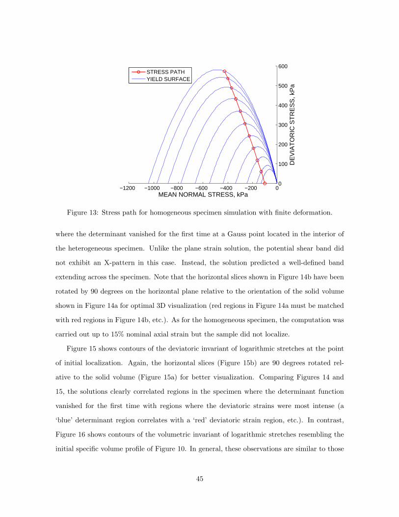
Figure 13 shows that this phase transition was captured by the constitutive model by first

yielding on the compression side of the yield surface, and later by yielding on the dilation

side.

Figure 14 shows contours of the determinant function F at a nominal axial strain of 8.78%,

43

0100

2 4 6 8 10

200

300

400

NOMINAL AXIAL STRAIN, %

NO

MIN

AL

AX

IAL

ST

RE

SS

, k

Pa

HOMOGENEOUS

HETEROGENEOUS

LOCALIZATION

Figure 11: Nominal axial stress-axial strain responses for 3D compression problem.

0 2 4 6 8 10

NOMINAL AXIAL STRAIN, %

VO

LU

ME

CH

AN

GE

, c

u.m

.

HOMOGENEOUS

HETEROGENEOUS

LOCALIZATION

− 0.01

− 0.02

0.00

− 0.03

− 0.04

Figure 12: Volume change-nominal axial strain responses for 3D compression problem.

44

−1200 −1000 −800 −600 −400 −200 00

100

200

300

400

500

600

MEAN NORMAL STRESS, kPa

DE

VIA

TO

RIC

ST

RE

SS

, kP

a

STRESS PATHYIELD SURFACE

Figure 13: Stress path for homogeneous specimen simulation with finite deformation.

where the determinant vanished for the first time at a Gauss point located in the interior of

the heterogeneous specimen. Unlike the plane strain solution, the potential shear band did

not exhibit an X-pattern in this case. Instead, the solution predicted a well-defined band

extending across the specimen. Note that the horizontal slices shown in Figure 14b have been

rotated by 90 degrees on the horizontal plane relative to the orientation of the solid volume

shown in Figure 14a for optimal 3D visualization (red regions in Figure 14a must be matched

with red regions in Figure 14b, etc.). As for the homogeneous specimen, the computation was

carried out up to 15% nominal axial strain but the sample did not localize.

Figure 15 shows contours of the deviatoric invariant of logarithmic stretches at the point

of initial localization. Again, the horizontal slices (Figure 15b) are 90 degrees rotated rel-

ative to the solid volume (Figure 15a) for better visualization. Comparing Figures 14 and

15, the solutions clearly correlated regions in the specimen where the determinant function

vanished for the first time with regions where the deviatoric strains were most intense (a

‘blue’ determinant region correlates with a ‘red’ deviatoric strain region, etc.). In contrast,

Figure 16 shows contours of the volumetric invariant of logarithmic stretches resembling the

initial specific volume profile of Figure 10. In general, these observations are similar to those

45

0

0.5

1

0

0.5

1

0

0.5

1

1.5

x−axisy−axis

z−axis

0

0.5

1 0

0.5

1

0

0.5

1

1.5

y−axisx−axisz−axis

0.5

1

1.5

2

2.5

3

x 1010

(a) (b)

Figure 14: Determinant function at onset of localization.

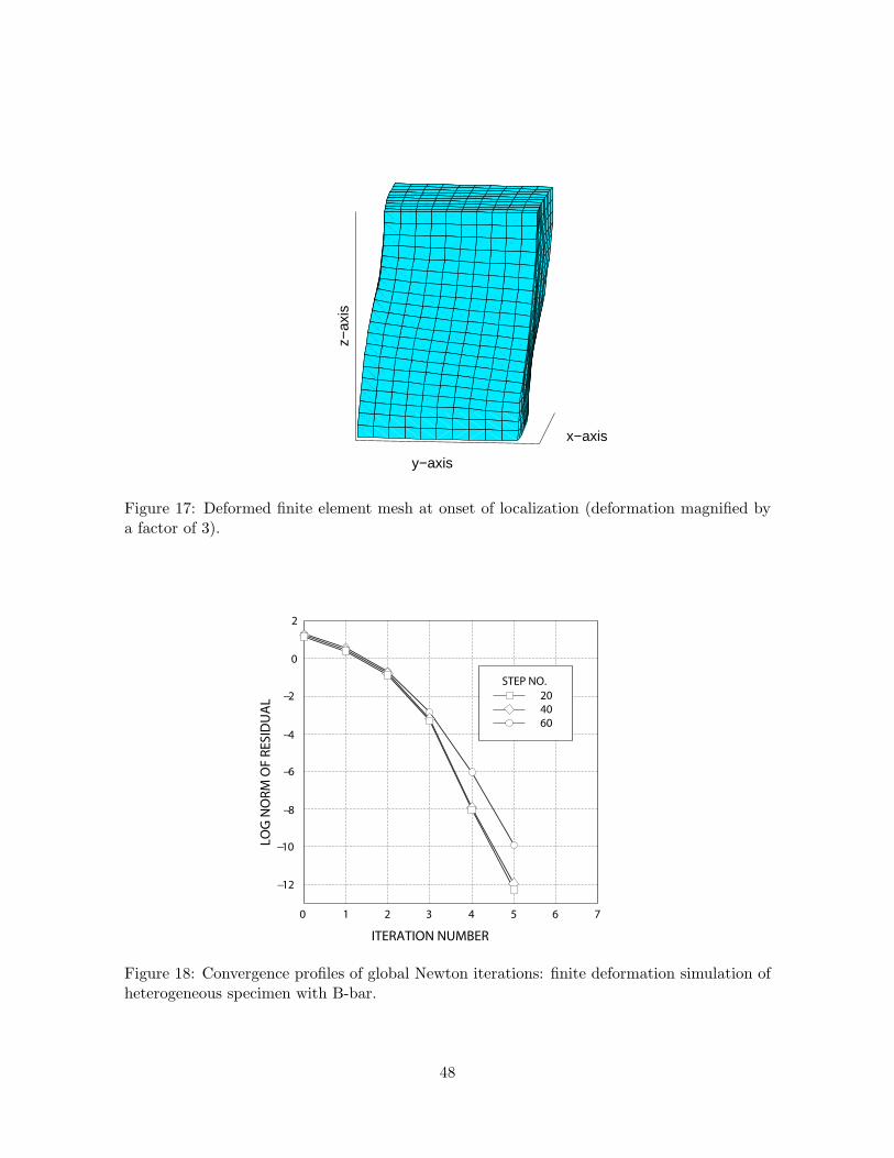
observed for the plane strain example. For completeness, Figure 17 shows the deformed FE

mesh for the heterogeneous sample at the instant of initial localization, suggesting that the

specimen moved laterally as well as twisted torsionally. Note once again that this non-uniform

deformation was triggered by the imposed initial density variation alone.

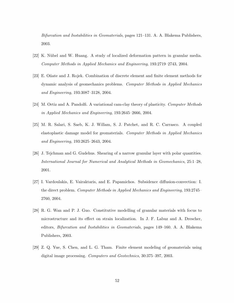
Finally, Figure 18 shows the convergence profiles of global Newton iterations for the full

3D finite deformation simulation of a heterogeneous specimen with B-bar integration. The

iterations converged quadratically in all cases, suggesting optimal performance. We empha-

size that all of the results presented above only pertain to the prediction of when and where

a potential shear band will emerge. We have not pursued the simulations beyond the point

of bifurcation due to mesh sensitivity issues inherent in rate-independent classical plasticity

models in the post-localized regime. A host of regularization techniques either in the consti-

tutive description or finite element solution are available and should be used to advance the

solution to this regime.

46

0

0.5

1

0

0.5

1

0

0.5

1

1.5

x−axisy−axis

z−axis

0

0.5

1 0

0.5

1

0

0.5

1

1.5

y−axisx−axisz−axis

0.03

0.04

0.05

0.06

0.07

0.08

0.09

0.1

0.11

0.12

(a) (b)

Figure 15: Deviatoric invariant of logarithmic stretches at onset of strain localization.

0

0.5

1

0

0.5

1

0

0.5

1

1.5

x−axisy−axis

z−axis

0

0.5

1 0

0.5

1

0

0.5

1

1.5

y−axisx−axis

z−axis

−0.024

−0.022

−0.02

−0.018

−0.016

−0.014

−0.012

−0.01

(a) (b)

Figure 16: Volumetric invariant of logarithmic stretches at onset of strain localization.

47

x−axis

y−axis

z−ax

is

Figure 17: Deformed finite element mesh at onset of localization (deformation magnified bya factor of 3).

20

40

60

STEP NO.

ITERATION NUMBER

0 1 2 3 4 5 6 7

0

− 2

− 4

− 6

− 8

− 10

− 12

2

LO

G N

OR

M O

F R

ES

IDU

AL

Figure 18: Convergence profiles of global Newton iterations: finite deformation simulation ofheterogeneous specimen with B-bar.

48

5 Closure

We have presented a meso-scale finite element modeling approach for capturing deformation

and strain localization in dense granular materials using critical state plasticity theory and

nonlinear finite element analysis. This approach has been motivated in large part by recent

trends in geotechnical laboratory testing allowing accurate quantitative measurement of the

spatial density variation in discrete granular materials. The meso-scale approach provides a

more realistic mathematical representation of imperfection; hence, it is expected to provide a

more thorough capture of the deformation and strain localization processes in these materials.

Potential extensions of the studies include a three-invariant enhancement of the plasticity

model and application of the model to unstructured random density fields (in contrast to the

structured density fields simulated in this paper). These aspects will be reported upon in a

future publication.

Acknowledgments

This work has been supported by National Science Foundation under Grant Nos. CMS-

0201317 and CMS-0324674 to Stanford University. We thank Professor Jack Baker of Stanford

University for his assistance in generating the initial specific volume profiles used in the

numerical examples, and Professor Amy Rechenmacher of USC for providing the X-Ray CT

image shown in Figure 1. We also thank the two anonymous reviewers for their constructive

reviews.

References

[1] J. Desrues and G. Viggiani. Strain localization in sand: an overview of the experimen-

tal results obtained in grenoble using stereophotogrammetry. International Journal for

Numerical and Analytical Methods in Geomechanics, 28:279–321, 2004.

[2] A. L. Rechenmacher and R. J. Finno. Digital image correlation to evaluate shear banding

in dilative sands. Geotechnical Testing Jounal, ASCE, 27:1–10, 2004.

49

[3] A. L. Rechenmacher and R. J. Finno. Shear band displacements and void ratio evolution

to critical state in dilative sands. In J. F. Labuz and A. Drescher, editors, Bifurcation

and Instabilities in Geomaterials, pages 13–22. A. A. Blakema Publishers, 2003.

[4] K. A. Alshibli, S. Sture, N. C. Costes, M. L. Frank, F. R. Lankton, S. N. Batiste, and

R. A. Swanson. Assessment of localized deformations in sand using x-ray computed

tomography. Geotechnical Testing Journal, ASCE, 23:274–299, 2000.

[5] K. A. Alshibli and S. Sture. Shear band formation in plane strain compression. Journal

of Geotechnical and Geoenvironmental Engineering, ASCE, 126:495–503, 2000.

[6] K. A. Alshibli, S. N. Batiste, and S. Sture. Strain localization in sand: plane strain

versus triaxial compression. Journal of Geotechnical and Geoenvironmental Engineering,

ASCE, 129:483–494, 2003.

[7] J. Desrues, R. Chambon, M. Mokni, and F. Mazerolle. Void ratio evolution inside

shear bands in triaxial sand specimens studied by computed tomography. Geotechnique,

46:527–546, 1996.

[8] R. J. Finno, W. W. Harris, and M. A. Mooney. Strain localization and undrained steady

state of sands. Journal of Geotechnical Engineering, ASCE, 122:462–473, 1996.

[9] G. Gudehus and K. Nubel. Evolution of shear bands in sand. Geotechnique, 54:187–201,

2004.

[10] I. Vardoulakis, M. Goldscheider, and G. Gudehus. Formation of shear bands in sand

bodies as a bifurcation problem. International Journal for Numerical and Analytical

Methods Geomechanics, 2:99–128, 1978.

[11] I. Vardoulakis and B. Graf. Calibration of constitutive models for granular materials

using data from biaxial experiments. Geotechnique, 35:299–317, 1985.

[12] E. Bauer, W. Wu, and W. Huang. Influence of an initially transverse isotropy on shear

banding in granular materials. In J. F. Labuz and A. Drescher, editors, Bifurcation and

Instabilities in Geomaterials, pages 161–172. A. A. Blakema Publishers, 2003.

50

[13] R. I. Borja and T. Y. Lai. Propagation of localization instability under active and passive

loading. Journal of Geotechnical and Geoenvironmental Engineering, ASCE, 128:64–75,

2002.

[14] R. Chambon and J. C. Moullet. Uniqueness studies in boundary value problems involving

some second gradient models. Computer Methods in Applied Mechanics and Engineering,

193:2771–2796, 2004.

[15] R. Chambon, D. Caillerie, and C. Tamagnini. A strain space gradient plasticity theory for

finite strain. Computer Methods in Applied Mechanics and Engineering, 193:2797–2826,

2004.

[16] F. Darve, G. Servant, F. Laouafa, and H. D. V. Khoa. Failure in geomaterials: contin-

uous and discrete analyses. Computer Methods in Applied Mechanics and Engineering,

193:3057–3085, 2004.

[17] R. de Borst and H. B. Muhlhaus. Gradient-dependent plasticity: Formulation and algo-

rithmic aspects. International Journal for Numerical Methods in Engineering, 35:521–

539, 1992.

[18] A. Gajo, D. Bigoni, and D. M. Wood. Stress induced elastic anisotropy and strain

localisation in sand. In H. B. Muhlhaus, A. Dyskin, and E. Pasternak, editors, Bifurcation

and Localisation Theory in Geomechanics, pages 37–44. A. A. Blakema Publishers, 2001.

[19] S. Kimoto, F. Oka, and Y. Higo. Strain localization analysis of elasto-viscoplastic soil

considering structural degradation. Computer Methods in Applied Mechanics and Engi-

neering, 193:2845–2866, 2004.

[20] P. A. Klerck, E. J. Sellers, and D. R. J. Owen. Discrete fracture in quasi-brittle materials

under compressive and tensile stress states. Computer Methods in Applied Mechanics

and Engineering, 193:3035–3056, 2004.

[21] B. Muhunthan, O. Alhattamleh, and H. M. Zbib. Modeling of localization in granular

materials: effect of porosity and particle size. In J. F. Labuz and A. Drescher, editors,

51

Bifurcation and Instabilities in Geomaterials, pages 121–131. A. A. Blakema Publishers,

2003.

[22] K. Nubel and W. Huang. A study of localized deformation pattern in granular media.

Computer Methods in Applied Mechanics and Engineering, 193:2719–2743, 2004.

[23] E. Onate and J. Rojek. Combination of discrete element and finite element methods for

dynamic analysis of geomechanics problems. Computer Methods in Applied Mechanics

and Engineering, 193:3087–3128, 2004.

[24] M. Ortiz and A. Pandolfi. A variational cam-clay theory of plasticity. Computer Methods

in Applied Mechanics and Engineering, 193:2645–2666, 2004.

[25] M. R. Salari, S. Saeb, K. J. Willam, S. J. Patchet, and R. C. Carrasco. A coupled

elastoplastic damage model for geomaterials. Computer Methods in Applied Mechanics

and Engineering, 193:2625–2643, 2004.

[26] J. Tejchman and G. Gudehus. Shearing of a narrow granular layer with polar quantities.

International Journal for Numerical and Analytical Methods in Geomechanics, 25:1–28,

2001.

[27] I. Vardoulakis, E. Vairaktaris, and E. Papamichos. Subsidence diffusion-convection: I.

the direct problem. Computer Methods in Applied Mechanics and Engineering, 193:2745–

2760, 2004.

[28] R. G. Wan and P. J. Guo. Constitutive modelling of granular materials with focus to

microstructure and its effect on strain localization. In J. F. Labuz and A. Drescher,

editors, Bifurcation and Instabilities in Geomaterials, pages 149–160. A. A. Blakema

Publishers, 2003.

[29] Z. Q. Yue, S. Chen, and L. G. Tham. Finite element modeling of geomaterials using

digital image processing. Computers and Geotechnics, 30:375–397, 2003.

52

[30] K. H. Roscoe and J. H. Burland. On the generalized stress–strain behavior of ‘wet’

clay. In J. Heyman and F. A. Leckie, editors, Engineering Plasticity, pages 535–609.

Cambridge University Press, 1968.

[31] A. Schofield and P. Wroth. Critical State Soil Mechanics. McGraw-Hill, New York, 1968.

[32] R. I. Borja and S. R. Lee. Cam-Clay plasticity, Part I: Implicit integration of elasto-

plastic constitutive relations. Computer Methods in Applied Mechanics and Engineering,

78:49–72, 1990.

[33] R. I. Borja. Cam-Clay plasticity, Part II: Implicit integration of constitutive equation

based on nonlinear elastic stress predictor. Computer Methods in Applied Mechanics and

Engineering, 88:225–240, 1991.

[34] R. I. Borja and C. Tamagnini. Cam-Clay plasticity, Part III: Extension of the in-

finitesimal model to include finite strains. Computer Methods in Applied Mechanics and

Engineering, 155:73–95, 1998.

[35] D. Peric and M.A. Ayari. Influence of Lode’s angle on the pore pressure generation in

soils. International Journal of Plasticity, 18:1039–1059, 2002.

[36] D. Peric and M.A. Ayari. On the analytical solutions for the three-invariant Cam clay

model. International Journal of Plasticity, 18:1061–1082, 2002.

[37] K. Been and M. G. Jefferies. A state parameter for sands. Geotechnique, 35:99–112,

1985.

[38] M. G. Jefferies. Nor-Sand: a simple critical state model for sand. Geotechnique, 43:91–

103, 1993.

[39] M. T. Manzari and Y. F. Dafalias. A critical state two-surface plasticity model for sands.

Geotechnique, 43:255–272, 1997.

[40] K. Ishihara, F. Tatsuoka, and S. Yasuda. Undrained deformation and liquefaction of

sand under cyclic stresses. Soils and Foundations, 15:29–44, 1975.

53

[41] S. L. Kramer. Geotechnical Earthquake Engineering. Prentice-Hall, New Jersey, 1996.

[42] A. Gens and D.M. Potts. Critical state models in computational geomechanics. Engi-

neering Computations, 5:178–197, 1988.

[43] R. J. Jardine, D. M. Potts, A. B. Fourie, and J. B. Burland. Studies of the influence of

non-linear stress-strain characteristics in soil-structure interaction. Geotechnique, 36:377–

396, 1986.

[44] G. T. Houlsby. The use of a variable shear modulus in elasto-plastic models for clays.

Computers and Geotechnics, 1:3–13, 1985.

[45] R. I. Borja, K. M. Sama, and P. F. Sanz. On the numerical integration of three-invariant

elastoplastic constitutive models. Computer Methods in Applied Mechanics and Engi-

neering, 192:1227–1258, 2003.

[46] P. V. Lade. Static instability and liquefaction of loose fine sandy slopes. Journal of

Geotechnical Engineering, ASCE, 118:51–71, 1992.

[47] J. C. Simo and T. J. R. Hughes. Computational Inelasticity. Prentice-Hall, New York,

1998.

[48] J. Sulem, I. Vardoulakis, E. Papamichos, A. Oulahna, and J. Tronvoll. Elasto-plastic

modelling of red wildmoor sandstone. Mechanics of Cohesive-Frictional Materials, 4:215–

245, 1999.

[49] R. I. Borja and A. Aydin. Computational modeling of deformation bands in granular me-

dia. I. Geological and mathematical framework. Computer Methods in Applied Mechanics

and Engineering, 193:2667–2698, 2004.

[50] R. I. Borja. Computational modeling of deformation bands in granular media. II.

Numerical simulations. Computer Methods in Applied Mechanics and Engineering,

193:2699–2718, 2004.

54

[51] E. H. Lee. Elastic-plastic deformation at finite strain. Journal of Applied Mechanics,

36:1–6, 1969.

[52] J. E. Marsden and T. J. R. Hughes. Mathematical Theory of Elasticity. Prentice-Hall,

Englewood Cliffs, NJ, 1983.

[53] L. E. Malvern. Introduction to the Mechanics of a Continuous Medium. Prentice-Hall,

Inc., Englewood Cliffs, NJ, 1969.

[54] J. C. Simo. Algorithms for static and dynamic multiplicative plasticity that preserve

the classical return mapping schemes of the infinitesimal theory. Computer Methods in

Applied Mechanics and Engineering, 99:61–112, 1992.

[55] Y. F. Dafalias. Plastic spin: necessity or redundancy? International Journal of Plasticity,

14:909–931, 1998.

[56] R. I. Borja. Bifurcation of elastoplastic solids to shear band mode at finite strains.

Computer Methods in Applied Mechanics and Engineering, 191:5287–5314, 2002.

[57] J. W. Rudnicki and J. R. Rice. Conditions for localization of deformation in pressure-

sensitive dilatant materials. Journal of the Mechanics and Physics of Solids, 23:371–394,

1975.

[58] T. J. R. Hughes. The Finite Element Method. Prentice-Hall, Englewood Cliffs, NJ, 1987.

[59] J. C. Nagtegaal, D. M. Parks, and J. R. Rice. On numerically accurate finite element

solutions in the fully plastic regime. Computer Methods in Applied Mechanics and Engi-

neering, 4:153–177, 1974.

[60] J. C. Simo, R. L. Taylor, and K. S. Pister. Variational and projection methods for the

volume constraint in finite deformation elasto-plasticity. Computer Methods in Applied

Mechanics and Engineering, 51:177–208, 1985.

55