critical state plasticity. part vi: meso-scale finite...
TRANSCRIPT
www.elsevier.com/locate/cma
Comput. Methods Appl. Mech. Engrg. 195 (2006) 5115–5140
Critical state plasticity. Part VI:Meso-scale finite element simulation of strain localization
in discrete granular materials
Ronaldo I. Borja *,1, Jose E. Andrade
Department of Civil and Environmental Engineering, Stanford University, Stanford, CA 94305, USA
Received 13 March 2005; received in revised form 30 August 2005; accepted 31 August 2005
Abstract
Development of more accurate mathematical models of discrete granular material behavior requires a fundamental understanding ofdeformation and strain localization phenomena. This paper utilizes a meso-scale finite element modeling approach to obtain an accurateand thorough capture of deformation and strain localization processes in discrete granular materials such as sands. We employ criticalstate theory and implement an elastoplastic constitutive model for granular materials, a variant of a model called ‘‘Nor-Sand’’, allowingfor non-associative plastic flow and formulating it in the finite deformation regime. Unlike the previous versions of critical state plasticitymodels presented in a series of ‘‘Cam-Clay’’ papers, the present model contains an additional state parameter w that allows for adeviation or detachment of the yield surface from the critical state line. Depending on the sign of this state parameter, the model canreproduce plastic compaction as well as plastic dilation in either loose or dense granular materials. Through numerical examples we dem-onstrate how a structured spatial density variation affects the predicted strain localization patterns in dense sand specimens.� 2005 Elsevier B.V. All rights reserved.
Keywords: Granular materials; Strain localization
1. Introduction
Development of accurate mathematical models of discrete granular material behavior requires a fundamental understand-ing of the localization phenomena, such as the formation of shear bands in dense sands. For this reason, much experimentalwork has been conducted to gain a better understanding of the localization process in these materials [1–11]. The subject alsohas spurred considerable interest in the theoretical and computational modeling fields [12–29]. It is important to recognizethat the material response observed in the laboratory is a result of many different micro-mechanical processes, such as mineralparticle rolling and sliding in granular soils, micro-cracking in brittle rocks, and mineral particle rotation and translation inthe cement matrix of soft rocks. Ideally, any localization model for geomaterials must represent all of these processes. How-ever, current limitations of experimental and mathematical modeling techniques in capturing the evolution in the micro-scalethroughout testing have inhibited the use of a micro-mechanical description of the localized deformation behavior.
To circumvent the problems associated with the micro-mechanical modeling approach, a macro-mechanical approach isoften used. For soils, this approach pertains to the specimen being considered as a macro-scale element from which thematerial response may be inferred. The underlying assumption is that the specimen is prepared uniformly and deformed
0045-7825/$ - see front matter � 2005 Elsevier B.V. All rights reserved.
doi:10.1016/j.cma.2005.08.020
* Corresponding author. Fax: +1 650 723 7514.E-mail address: [email protected] (R.I. Borja).
1 Supported by US National Science Foundation, Grant Nos. CMS-0201317 and CMS-0324674.
5116 R.I. Borja, J.E. Andrade / Comput. Methods Appl. Mech. Engrg. 195 (2006) 5115–5140
homogeneously enough to allow extraction of the material response from the specimen response. However, it is well knownthat each specimen is unique, and that two identically prepared samples could exhibit different mechanical responses in theregime of instability even if they had been subjected to the same initially homogeneous deformation field. This implies thatthe size of a specimen is too large to accurately resolve the macro-scale field, and that it can only capture the strain local-ization phenomena in a very approximate way.
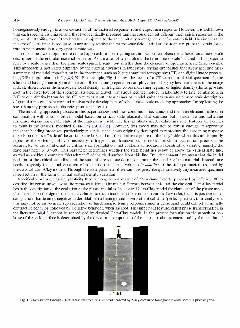
In this paper, we adopt a more refined approach to investigating strain localization phenomena based on a meso-scaledescription of the granular material behavior. As a matter of terminology, the term ‘‘meso-scale’’ is used in this paper torefer to a scale larger than the grain scale (particle scale) but smaller than the element, or specimen, scale (macro-scale).This approach is motivated primarily by the current advances in laboratory testing capabilities that allow accurate mea-surements of material imperfection in the specimens, such as X-ray computed tomography (CT) and digital image process-ing (DIP) in granular soils [1,4,8,9,29]. For example, Fig. 1 shows the result of a CT scan on a biaxial specimen of puresilica sand having a mean grain diameter of 0.5 mm and prepared via air pluviation. The gray level variations in the imageindicate differences in the meso-scale local density, with lighter colors indicating regions of higher density (the large whitespot in the lower level of the specimen is a piece of gravel). This advanced technology in laboratory testing, combined withDIP to quantitatively transfer the CT results as input into a numerical model, enhances an accurate meso-scale descriptionof granular material behavior and motivates the development of robust meso-scale modeling approaches for replicating theshear banding processes in discrete granular materials.
The modeling approach pursued in this paper utilizes nonlinear continuum mechanics and the finite element method, incombination with a constitutive model based on critical state plasticity that captures both hardening and softeningresponses depending on the state of the material at yield. The first plasticity model exhibiting such features that comesto mind is the classical modified Cam-Clay [24,30–36]. However, this model may not be robust enough to reproducethe shear banding processes, particularly in sands, since it was originally developed to reproduce the hardening responseof soils on the ‘‘wet’’ side of the critical state line, and not the dilative response on the ‘‘dry’’ side where this model poorlyreplicates the softening behavior necessary to trigger strain localization. To model the strain localization process moreaccurately, we use an alternative critical state formulation that contains an additional constitutive variable, namely, thestate parameter w [37–39]. This parameter determines whether the state point lies below or above the critical state line,as well as enables a complete ‘‘detachment’’ of the yield surface from this line. By ‘‘detachment’’ we mean that the initialposition of the critical state line and the state of stress alone do not determine the density of the material. Instead, oneneeds to specify the spatial variation of void ratio (or specific volume) in addition to the state parameters required bythe classical Cam-Clay models. Through the state parameter w we can now prescribe quantitatively any measured specimenimperfection in the form of initial spatial density variation.
Specifically, we use classical plasticity theory along with a variant of ‘‘Nor-Sand’’ model proposed by Jefferies [38] todescribe the constitutive law at the meso-scale level. The main difference between this and the classical Cam-Clay modellies in the description of the evolution of the plastic modulus. In classical Cam-Clay model the character of the plastic mod-ulus depends on the sign of the plastic volumetric strain increment (determined from the flow rule), i.e., it is positive undercompaction (hardening), negative under dilation (softening), and is zero at critical state (perfect plasticity). In sandy soilsthis may not be an accurate representation of hardening/softening responses since a dense sand could exhibit an initiallycontractive behavior, followed by a dilative behavior, when sheared. This important feature, called phase transformation inthe literature [40,41], cannot be reproduced by classical Cam-Clay models. In the present formulation the growth or col-lapse of the yield surface is determined by the deviatoric component of the plastic strain increment and by the position of
Fig. 1. Cross-section through a biaxial test specimen of silica sand analyzed by X-ray computed tomography; white spot is a piece of gravel.
R.I. Borja, J.E. Andrade / Comput. Methods Appl. Mech. Engrg. 195 (2006) 5115–5140 5117
the stress point relative to a so-called limit hardening dilatancy. Such description reproduces more accurately the softeningresponse on the ‘‘dry’’ side of the critical state line.
The theoretical and computational aspects of this paper include the mathematical analyses of the thermodynamics ofconstitutive models characterized by elastoplastic coupling [42,43]. We also describe the numerical implementation ofthe finite deformation version of the model, the impact of B-bar integration near the critical state, and the localizationof deformation on the ‘‘dry’’ side of the critical state line. We present two numerical examples demonstrating the locali-zation of deformation in plane strain and full 3D loading conditions, highlighting in both cases the important role thatthe spatial density variation plays on the mechanical responses of dense granular materials.
Notations and symbols used in this paper are as follows: bold-faced letters denote tensors and vectors; the symbol ‘Æ’denotes an inner product of two vectors (e.g. a Æ b = aibi), or a single contraction of adjacent indices of two tensors (e.g.c Æ d = cijdjk); the symbol ‘:’ denotes an inner product of two second-order tensors (e.g. c : d = cijdij), or a double contractionof adjacent indices of tensors of rank two and higher (e.g. C : �e ¼ Cijkl�
ekl); the symbol ‘�’ denotes a juxtaposition, e.g.,
(a � b)ij = aibj. Finally, for any symmetric second-order tensors a and b, (a � b)ijkl = aijbkl, (a � b)ijkl = ajlbik, and(a � b)ijkl = ailbjk.
2. Formulation of the infinitesimal model
We begin by presenting the general features of the meso-scale constitutive model in the infinitesimal regime. Extensionof the features to the finite deformation regime is then presented in the next section.
2.1. Hyperelastic response
We consider a stored energy density function We(�e) in a granular assembly taken as a continuum; the macroscopic stressr is given by
r ¼ oWe
o�e; ð2:1Þ
where
We ¼ eWeð�evÞ þ
3
2le�e2
s ; ð2:2Þ
and eWð�evÞ ¼ �p0~j exp x; x ¼ � �
ev � �e
v0
~j; le ¼ l0 þ
a0
~jeWð�e
vÞ. ð2:3Þ
The independent variables are the infinitesimal macroscopic volumetric and deviatoric strain invariants
�ev ¼ trð�eÞ; �e
s ¼ffiffiffi2
3
rkeek; ee ¼ �e � 1
3�e
v1; ð2:4Þ
where �e is the elastic component of the infinitesimal macroscopic strain tensor. The material parameters required for def-inition are the reference strain �e
v0 and reference pressure p0 of the elastic compression curve, as well as the elastic compress-ibility index ~j. The above model produces pressure-dependent elastic bulk and shear moduli, in accord with a well-knownsoil behavioral feature. Eq. (2.3) results in a constant elastic shear modulus le = l0 when a0 = 0. This model is conservativein the sense that no energy is generated or lost in a closed elastic loading loop [44].
2.2. Yield surface, plastic potential function, and flow rule
We consider the first two stress invariants
p ¼ 1
3trr; q ¼
ffiffiffi3
2
rksk; s ¼ r� p1; ð2:5Þ
where p 6 0 in general. We define a yield function F of the form
F ¼ qþ gp; ð2:6Þwhere
g ¼M ½1þ lnðpi=pÞ� if N ¼ 0;
ðM=NÞ½1� ð1� NÞðp=piÞN=ð1�NÞ� if N > 0.
(ð2:7Þ
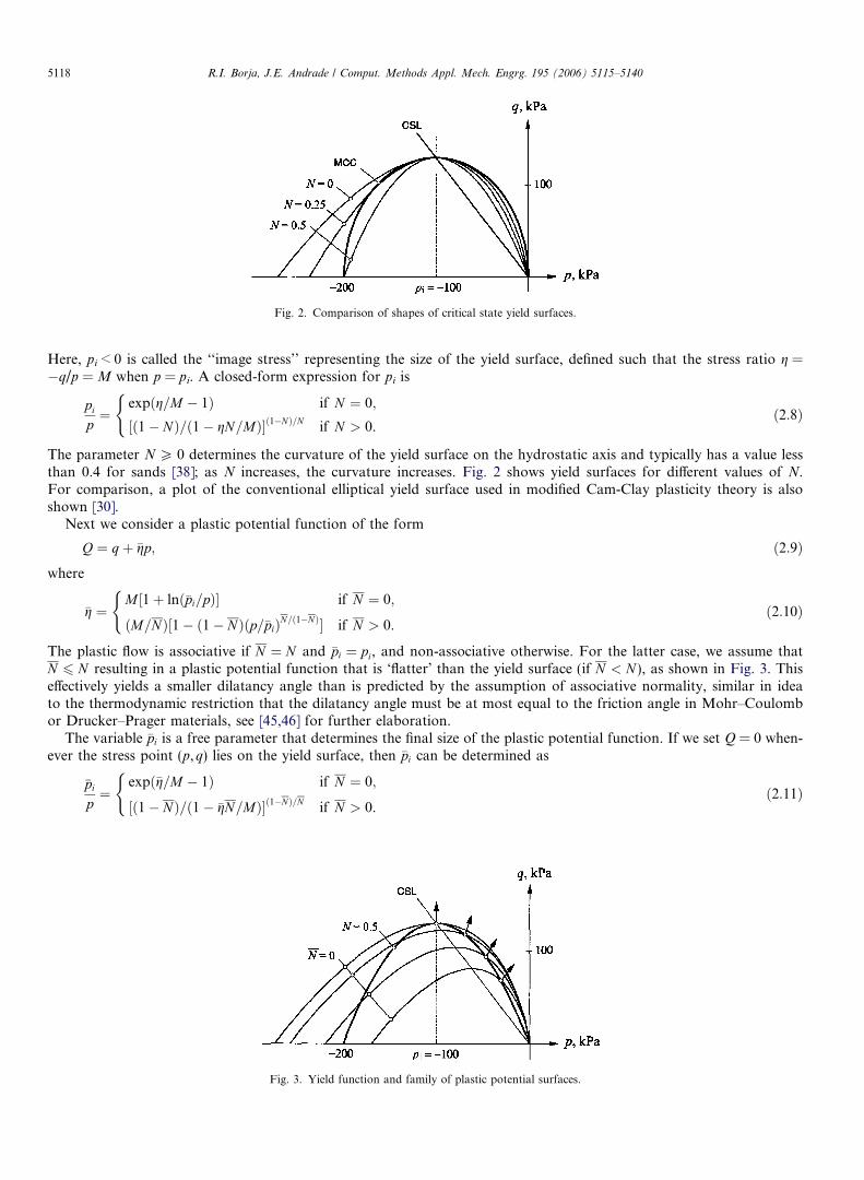
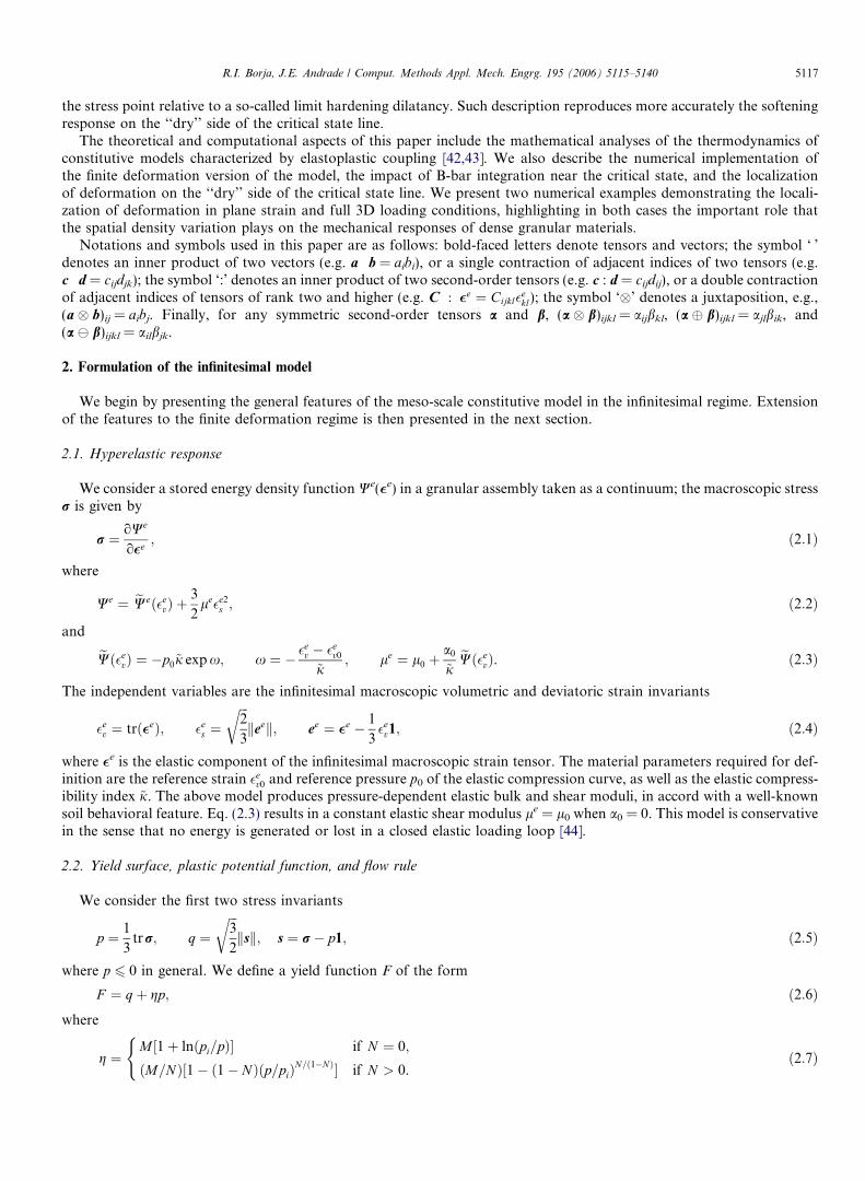
Fig. 2. Comparison of shapes of critical state yield surfaces.
5118 R.I. Borja, J.E. Andrade / Comput. Methods Appl. Mech. Engrg. 195 (2006) 5115–5140
Here, pi < 0 is called the ‘‘image stress’’ representing the size of the yield surface, defined such that the stress ratio g =�q/p = M when p = pi. A closed-form expression for pi is
pi
p¼
expðg=M � 1Þ if N ¼ 0;
½ð1� NÞ=ð1� gN=MÞ�ð1�NÞ=N if N > 0.
(ð2:8Þ
The parameter N P 0 determines the curvature of the yield surface on the hydrostatic axis and typically has a value lessthan 0.4 for sands [38]; as N increases, the curvature increases. Fig. 2 shows yield surfaces for different values of N.For comparison, a plot of the conventional elliptical yield surface used in modified Cam-Clay plasticity theory is alsoshown [30].
Next we consider a plastic potential function of the form
Q ¼ qþ �gp; ð2:9Þwhere
�g ¼M ½1þ lnð�pi=pÞ� if N ¼ 0;
ðM=NÞ½1� ð1� NÞðp=�piÞN=ð1�NÞ� if N > 0.
(ð2:10Þ
The plastic flow is associative if N ¼ N and �pi ¼ pi, and non-associative otherwise. For the latter case, we assume thatN 6 N resulting in a plastic potential function that is ‘flatter’ than the yield surface (if N < N ), as shown in Fig. 3. Thiseffectively yields a smaller dilatancy angle than is predicted by the assumption of associative normality, similar in ideato the thermodynamic restriction that the dilatancy angle must be at most equal to the friction angle in Mohr–Coulombor Drucker–Prager materials, see [45,46] for further elaboration.
The variable �pi is a free parameter that determines the final size of the plastic potential function. If we set Q = 0 when-ever the stress point (p,q) lies on the yield surface, then �pi can be determined as
�pi
p¼
expð�g=M � 1Þ if N ¼ 0;
½ð1� NÞ=ð1� �gN=MÞ�ð1�NÞ=N if N > 0.
(ð2:11Þ
Fig. 3. Yield function and family of plastic potential surfaces.
R.I. Borja, J.E. Andrade / Comput. Methods Appl. Mech. Engrg. 195 (2006) 5115–5140 5119
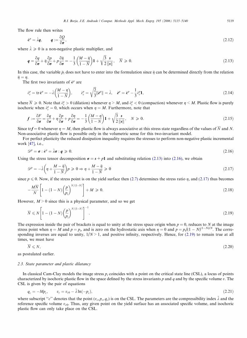
The flow rule then writes
_�p ¼ _kq; q :¼ oQor
; ð2:12Þ
where _k P 0 is a non-negative plastic multiplier, and
q ¼ oqorþ �g
oporþ p
o�gor¼ � 1
3
M � �g
1� N
� �1þ
ffiffiffi3
2
rs
ksk ; N P 0. ð2:13Þ
In this case, the variable �pi does not have to enter into the formulation since �g can be determined directly from the relation�g ¼ g.
The first two invariants of _�p are
_�pv ¼ tr _�p ¼ � _k
M � g
1� N
� �; _�p
s ¼ffiffiffi2
3
rk_epk ¼ _k; _ep ¼ _�p � 1
3_�p
v1; ð2:14Þ
where N P 0. Note that _�pv > 0 (dilation) whenever g > M, and _�p
v < 0 (compaction) whenever g < M. Plastic flow is purelyisochoric when _�p
v ¼ 0, which occurs when g = M. Furthermore, note that
f :¼ oFor¼ oq
orþ g
oporþ p
ogor¼ � 1
3
M � g1� N
� �1þ
ffiffiffi3
2
rs
ksk ; N P 0. ð2:15Þ
Since tr f = 0 whenever g = M, then plastic flow is always associative at this stress state regardless of the values of N and N.Non-associative plastic flow is possible only in the volumetric sense for this two-invariant model.
For perfect plasticity the reduced dissipation inequality requires the stresses to perform non-negative plastic incrementalwork [47], i.e.,
Dp ¼ r : _�p ¼ _kr : q P 0. ð2:16ÞUsing the stress tensor decomposition r = s + p1 and substituting relation (2.13) into (2.16), we obtain
Dp ¼ � _k gþM � �g
1� N
� �p P 0) gþM � �g
1� NP 0 ð2:17Þ
since p 6 0. Now, if the stress point is on the yield surface then (2.7) determines the stress ratio g, and (2.17) thus becomes
�MNN
1� ð1� NÞ ppi
� �N=ð1�NÞ" #
þM P 0. ð2:18Þ
However, M > 0 since this is a physical parameter, and so we get
N 6 N 1� ð1� NÞ ppi
� �N=ð1�NÞ" #�1
. ð2:19Þ
The expression inside the pair of brackets is equal to unity at the stress space origin when p = 0, reduces to N at the imagestress point when g = M and p = pi, and is zero on the hydrostatic axis when g = 0 and p = pi/(1 � N)(1�N)/N. The corre-sponding inverses are equal to unity, 1/N > 1, and positive infinity, respectively. Hence, for (2.19) to remain true at alltimes, we must have
N 6 N ; ð2:20Þas postulated earlier.
2.3. State parameter and plastic dilatancy
In classical Cam-Clay models the image stress pi coincides with a point on the critical state line (CSL), a locus of pointscharacterized by isochoric plastic flow in the space defined by the stress invariants p and q and by the specific volume v. TheCSL is given by the pair of equations
qc ¼ �Mpc; vc ¼ vc0 � ~k lnð�pcÞ; ð2:21Þwhere subscript ‘‘c’’ denotes that the point (vc,pc,qc) is on the CSL. The parameters are the compressibility index ~k and thereference specific volume vc0. Thus, any given point on the yield surface has an associated specific volume, and isochoricplastic flow can only take place on the CSL.
5120 R.I. Borja, J.E. Andrade / Comput. Methods Appl. Mech. Engrg. 195 (2006) 5115–5140
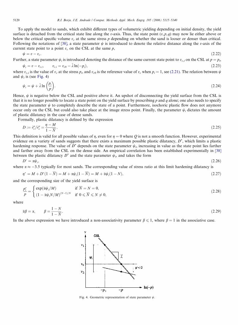
To apply the model to sands, which exhibit different types of volumetric yielding depending on initial density, the yieldsurface is detached from the critical state line along the v-axis. Thus, the state point (v,p,q) may now lie either above orbelow the critical specific volume vc at the same stress p depending on whether the sand is looser or denser than critical.Following the notations of [38], a state parameter w is introduced to denote the relative distance along the v-axis of thecurrent state point to a point vc on the CSL at the same p,
w ¼ v� vc. ð2:22ÞFurther, a state parameter wi is introduced denoting the distance of the same current state point to vc,i on the CSL at p = pi,
wi ¼ v� vc;i; vc;i ¼ vc0 � ~k lnð�piÞ; ð2:23Þwhere vc,i is the value of vc at the stress pi, and vc0 is the reference value of vc when pi = 1, see (2.21). The relation between wand wi is (see Fig. 4)
wi ¼ wþ ~k lnpi
p
� �. ð2:24Þ
Hence, w is negative below the CSL and positive above it. An upshot of disconnecting the yield surface from the CSL isthat it is no longer possible to locate a state point on the yield surface by prescribing p and q alone; one also needs to specifythe state parameter w to completely describe the state of a point. Furthermore, isochoric plastic flow does not anymoreoccur only on the CSL but could also take place at the image stress point. Finally, the parameter wi dictates the amountof plastic dilatancy in the case of dense sands.
Formally, plastic dilatancy is defined by the expression
D :¼ _�pv=_�p
s ¼g�M
1� N. ð2:25Þ
This definition is valid for all possible values of g, even for g = 0 where Q is not a smooth function. However, experimentalevidence on a variety of sands suggests that there exists a maximum possible plastic dilatancy, D*, which limits a plastichardening response. The value of D* depends on the state parameter wi, increasing in value as the state point lies fartherand farther away from the CSL on the dense side. An empirical correlation has been established experimentally in [38]between the plastic dilatancy D* and the state parameter wi, and takes the form
D� ¼ awi; ð2:26Þwhere a � �3.5 typically for most sands. The corresponding value of stress ratio at this limit hardening dilatancy is
g� ¼ M þ D�ð1� NÞ ¼ M þ awið1� NÞ ¼ M þ �awið1� NÞ; ð2:27Þand the corresponding size of the yield surface is
p�ip¼
expð�awi=MÞ if N ¼ N ¼ 0;
ð1� �awiN=MÞðN�1Þ=N if 0 6 N 6 N 6¼ 0;
(ð2:28Þ
where
�ab ¼ a; b ¼ 1� N
1� N. ð2:29Þ
In the above expression we have introduced a non-associativity parameter b 6 1, where b = 1 in the associative case.
Fig. 4. Geometric representation of state parameter w.
R.I. Borja, J.E. Andrade / Comput. Methods Appl. Mech. Engrg. 195 (2006) 5115–5140 5121
2.4. Consistency condition and hardening law
For elastoplastic response the standard consistency condition on the yield function F reads
_F ¼ f : _r� H _k ¼ 0; _k > 0; ð2:30Þwhere H is the plastic modulus given by the equation
H ¼ � 1_k
oFopi
_pi ¼ �1_k
ppi
� �1=ð1�NÞ
M _pi. ð2:31Þ
Since p/pi > 0, the sign of the plastic modulus depends on the sign of _pi : H > 0 if _pi < 0 (hardening), H < 0 if _pi > 0 (soft-ening), and H = 0 if _pi ¼ 0 (perfect plasticity).
In classical Cam-Clay theory the sign of H depends on the sign of _�pv , i.e., H is positive for compaction and negative for
expansion. However, as noted above, this simple criterion does not adequately capture the hardening/softening responsesof sands, which are shown to be dependent on the limit hardening plastic dilatancy D*, i.e., H is positive if D < D* andnegative if D > D*. Thus, any postulated hardening law must satisfy the obvious relationship
sgnH ¼ sgn ð� _piÞ ¼ sgn ðD� � DÞ ¼ sgn ðg� � gÞ ¼ sgn ðpi � p�i Þ; ð2:32Þwhere ‘sgn’ is the sign operator. Furthermore, in terms of the cumulative plastic shear strain
�ps ¼
Zt
_�ps dt; ð2:33Þ
we require that
lim�
ps!1
H ¼ lim�
ps!1ð� _piÞ ¼ lim
�ps!1ðD� � DÞ ¼ lim
�ps!1ðg� � gÞ ¼ lim
�ps!1ðpi � p�i Þ ¼ 0. ð2:34Þ
Thus, any postulated hardening law must reflect a condition of perfect plasticity as the plastic shear strain becomes verylarge. Note that the above restriction is stronger, e.g., than the weaker condition D* � D = 0, without the limit, whichcould occur even if the stress and image points do not coincide. The limiting condition �p
s !1 insures that the stressand image points approach the CSL, and that these two points coincide in the limit.
A general evolution for � _pi satisfying the requirements stated above may be given by an equation of the form
� _pi ¼ f ðpi � p�i Þ_�ps ¼ f ðpi � p�i Þ _k; ð2:35Þ
where f is a simple odd scalar function of its argument, i.e., f(�x) = �f(x) and sgn f = sgnx. (Alternately, one can use eitherD or g in the argument for f.) In this case, the expression for the plastic modulus becomes
H ¼ Mppi
� �1=ð1�NÞ
f ðpi � p�i Þ. ð2:36Þ
Taking f(x) = hx, where h is a positive dimensionless constant, we arrive at a phenomenological expression of the formsimilar to that presented in [38],
f ðpi � p�i Þ ¼ hðpi � p�i Þ. ð2:37Þ
This results in a plastic modulus given by the equation
H ¼ Mhppi
� �1=ð1�NÞ
ðpi � p�i Þ. ð2:38Þ
To summarize, the transition point between hardening and softening responses is represented by the limit hardening dilat-ancy D*, which approaches zero on the CSL.
2.5. Implications to entropy production
Consider the Helmholtz free energy density function W ¼ Wð�e; �ps Þ. For now, we avoid making the usual additive
decomposition of the free energy into W ¼ Weð�eÞ þWpð�ps Þ; in fact, we shall demonstrate that such decomposition is
not possible in the present model. Ignoring the non-mechanical powers, the local Clausius–Duhem inequality yields
r : _�� dWdt
P 0. ð2:39Þ
5122 R.I. Borja, J.E. Andrade / Comput. Methods Appl. Mech. Engrg. 195 (2006) 5115–5140
Applying the chain rule for dW/dt and invoking the standard Coleman relations results in the constitutive relation
r ¼ oWð�e; �ps Þ
o�e; ð2:40Þ
plus the reduced dissipation inequality
r : _�p � pi _�ps P 0; pi ¼
oWð�e; �ps Þ
o�ps
. ð2:41Þ
Here, we have chosen pi to be the stress-like plastic internal variable conjugate to �ps . With an appropriate set of material
parameters we have ensured before that r : _�p P 0 (see Section 2.2). Since _�ps ¼ _k P 0 and pi < 0, the reduced dissipation
inequality as written above holds provided that
oWð�e; �ps Þ
o�ps
6 0. ð2:42Þ
Now, consider the evolution for pi as postulated in (2.35). Integrating in time yields
oWð�e; �ps Þ
o�ps
pi ¼ pi0 �Z �
ps
�ps0
f ðpi � p�i Þd�ps ; ð2:43Þ
where pi0 is the reference value of pi when �ps ¼ �
ps0. Recalling that f is a simple odd function, the right-hand side of the above
equation is negative provided that sgn ðpi � p�i Þ ¼ sgnH ¼ positive. This implies that the reduced dissipation inequality isidentically satisfied in the hardening regime.
Integrating once more gives a more definitive form of the Helmholtz free energy,
Wð�e; �ps Þ ¼
Z �ps
�ps0
pi0d�ps �
Z �ps
�ps0
Z �ps
�ps0
f ðpi � p�i Þd�ps d�p
s þWeð�eÞ þW0; ð2:44Þ
where We(�e) is the usual elastic stored energy function. The first two integrals represent the plastic component of the freeenergy,
Wp ¼ Wpð�e; �ps Þ ¼
Z �ps
�ps0
pi0 d�ps �
Z �ps
�ps0
Z �ps
�ps0
f ðpi � p�i Þd�ps d�p
s . ð2:45Þ
Note in this case that Wp depends not only on �ps but also on �e through the variable p�i . The Cauchy stress tensor then
becomes
r ¼ oWeð�eÞo�e
þZ �
ps
�ps0
Z �ps
�ps0
f 0ðpi � p�i Þop�io�e
d�ps d�p
s|fflfflfflfflfflfflfflfflfflfflfflfflfflfflfflfflfflfflfflfflfflfflfflfflfflffl{zfflfflfflfflfflfflfflfflfflfflfflfflfflfflfflfflfflfflfflfflfflfflfflfflfflffl}OðD�p2
s Þ
; ð2:46Þ
where D�ps ¼ �p
s � �ps0, and
op�io�e¼ ð1� NÞ �ap�i =M
1� �awiN=Mowi
o�eþ p�i
popo�e
; N P 0. ð2:47Þ
Strictly, then, the Cauchy stress tensor depends not only on �e but also on �ps . Attempts have been made in the past to cap-
ture this dependence of r on �ps ; for example, a nonlinear elasticity model in which the elastic shear modulus varies with a
stress-like plastic internal variable similar to pi has been proposed in [43,48]. However, these developments have not gainedmuch acceptance in the literature due, primarily, to the lack of experimental data and to the difficulty with obtaining suchtest data.
It must be noted that the observed dependence of Wp on the elastic strain �e occurs only prior to reaching the criticalstate where D�p
s remains ‘‘relatively small’’, and thus, the second-order term in (2.46) may be ignored (such as done inSection 2.1). Most of the intense shearing (i.e., large D�p
s ) in fact occurs at the critical state where f ðpi � p�i Þ ¼ 0, at whichcondition the additive decomposition of the free energy into We(�e) and Wpð�p
s Þ holds, see (2.44).
2.6. Numerical implementation
Even though the plastic internal variable pi depends on the state parameter wi, and that this variable is deeply embeddedin the plastic modulus H, the model is still amenable to fully implicit numerical integration. Box 1 summarizes the relevantrate equations used in the constitutive theory. Box 2 summarizes the algorithmic counterpart utilizing the classical returnmapping scheme. For improved efficiency, the return mapping algorithm in Box 2 is performed in the strain invariant space,
1. Strain rates: _� ¼ _�e þ _�p.2. Hyperelastic rate equations: _r ¼ ce : _�e; ce = o2We/o�eo�e.3. Flow rule: _�p ¼ _kq.
4. State parameter: _wi ¼ _vþ ~k _pi=pi from (2.23).5. Hardening law: � _pi ¼ f ðpi � p�i Þ _k from (2.35).6. Consistency condition: f : _r� H _k ¼ 0.7. Kuhn–Tucker conditions: _k P 0, F 6 0 , _kF ¼ 0.
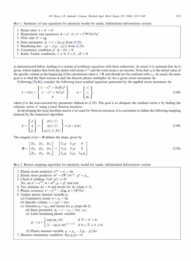
Box 1. Summary of rate equations for plasticity model for sands, infinitesimal deformation version
R.I. Borja, J.E. Andrade / Comput. Methods Appl. Mech. Engrg. 195 (2006) 5115–5140 5123
as demonstrated below, leading to a system of nonlinear equations with three unknowns. As usual, it is assumed that D� isgiven, which implies that both the elastic trial strain �e tr and the total strain � are known. Note that v0 is the initial value ofthe specific volume at the beginning of the calculations when � = 0, and should not be confused with vc0. As usual, the maingoal is to find the final stresses r and the discrete plastic multiplier Dk for a given strain increment D�.
Following [34,46], consider the following local residual equations generated by the applied strain increment D�
r ¼ rðxÞ ¼�e
v � �e trv þ DkbopF
�es � �e tr
s þ DkoqF
F
8><>:9>=>;; x ¼
�ev
�es
Dk
8><>:9>=>;; ð2:48Þ
where b is the non-associativity parameter defined in (2.29). The goal is to dissipate the residual vector r by finding thesolution vector x* using a local Newton iteration.
In developing the local Jacobian matrix r 0(x) used for Newton iteration, it is convenient to define the following mappinginduced by the numerical algorithm
y ¼p
q
pi
8><>:9>=>; ¼
pð�ev; �
esÞ
qð�ev; �
esÞ
pið�ev; �
es ;DkÞ
8><>:9>=>;) y ¼ yðxÞ. ð2:49Þ
The tangent y 0(x) = D defines the slope, given by
D ¼D11 D12 D13
D21 D22 D23
D31 D32 D33
264375 ¼ o�e
vp o�es p 0
o�ev q o�es q 0
o�ev pi o�es pi oDkpi
264375. ð2:50Þ
1. Elastic strain predictor: �e tr ¼ �en þ D�.
2. Elastic stress predictor: rtr ¼ oWe=o�e tr; ptri ¼ pi;n.
3. Check if yielding: F ðrtr; ptri ÞP 0?
No, set �e = �e tr; r = rtr; pi ¼ ptri and exit.
4. Yes, initialize Dk = 0 and iterate for Dk (steps 5–7).5. Plastic corrector: �e = �e tr � Dkq, r = oWe/o�e.6. Update plastic internal variable pi:
(a) Cumulative strain: � = �n + D�.(b) Specific volume: v = v0(1 + tr�).(c) Initialize pi = pi,n and iterate for pi (steps 6d–f).
(d) State parameter: wi ¼ v� vc0 þ ~k lnð�piÞ.(e) Limit hardening plastic variable:
p�i ¼ p expð�awi=MÞ if N ¼ N ¼ 0;
ð1� �awiN=MÞðN�1Þ=N if 0 6 N 6 N 6¼ 0.
((f) Plastic internal variable: pi ¼ pi;n � f ðpi � p�i ÞDk.
7. Discrete consistency condition: F(p,q,pi) = 0.
Box 2. Return mapping algorithm for plasticity model for sands, infinitesimal deformation version
5124 R.I. Borja, J.E. Andrade / Comput. Methods Appl. Mech. Engrg. 195 (2006) 5115–5140
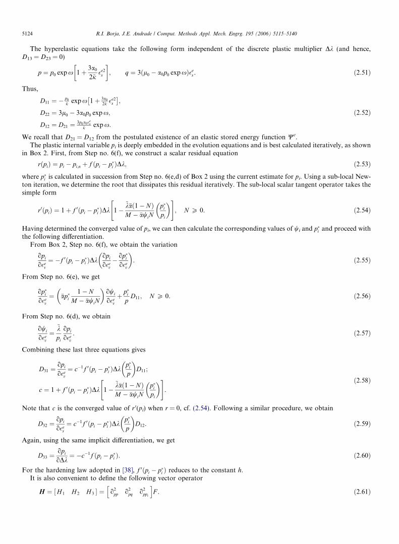
The hyperelastic equations take the following form independent of the discrete plastic multiplier Dk (and hence,D13 = D23 = 0)
p ¼ p0 exp x 1þ 3a0
2~j�e2
s
� �; q ¼ 3ðl0 � a0p0 exp xÞ�e
s . ð2:51Þ
Thus,
D11 ¼ � p0
~j exp x 1þ 3a0
2~j �e2s
� ;
D22 ¼ 3l0 � 3a0p0 exp x;
D12 ¼ D21 ¼ 3p0a0�es
~j exp x.
ð2:52Þ
We recall that D21 = D12 from the postulated existence of an elastic stored energy function We.The plastic internal variable pi is deeply embedded in the evolution equations and is best calculated iteratively, as shown
in Box 2. First, from Step no. 6(f), we construct a scalar residual equation
rðpiÞ ¼ pi � pi;n þ f ðpi � p�i ÞDk; ð2:53Þ
where p�i is calculated in succession from Step no. 6(e,d) of Box 2 using the current estimate for pi. Using a sub-local New-ton iteration, we determine the root that dissipates this residual iteratively. The sub-local scalar tangent operator takes thesimple form
r0ðpiÞ ¼ 1þ f 0ðpi � p�i ÞDk 1�~k�að1� NÞM � �awiN
p�ipi
� �" #; N P 0. ð2:54Þ
Having determined the converged value of pi, we can then calculate the corresponding values of wi and p�i and proceed withthe following differentiation.
From Box 2, Step no. 6(f), we obtain the variation
opi
o�ev
¼ �f 0ðpi � p�i ÞDkopi
o�ev
� op�io�e
v
� �. ð2:55Þ
From Step no. 6(e), we get
op�io�e
v
¼ �ap�i1� N
M � �awiN
� �owi
o�ev
þ p�ip
D11; N P 0. ð2:56Þ
From Step no. 6(d), we obtain
owi
o�ev
¼~kpi
opi
o�ev
. ð2:57Þ
Combining these last three equations gives
D31 ¼opi
o�ev
¼ c�1f 0ðpi � p�i ÞDkp�ip
� �D11;
c ¼ 1þ f 0ðpi � p�i ÞDk 1�~k�að1� NÞM � �awiN
p�ipi
� �" #.
ð2:58Þ
Note that c is the converged value of r 0(pi) when r = 0, cf. (2.54). Following a similar procedure, we obtain
D32 ¼opi
o�es
¼ c�1f 0ðpi � p�i ÞDkp�ip
� �D12. ð2:59Þ
Again, using the same implicit differentiation, we get
D33 ¼opi
oDk¼ �c�1f ðpi � p�i Þ. ð2:60Þ
For the hardening law adopted in [38], f 0ðpi � p�i Þ reduces to the constant h.It is also convenient to define the following vector operator
H ¼ H 1 H 2 H 3½ � ¼ o2pp o2
pq o2ppi
h iF . ð2:61Þ
R.I. Borja, J.E. Andrade / Comput. Methods Appl. Mech. Engrg. 195 (2006) 5115–5140 5125
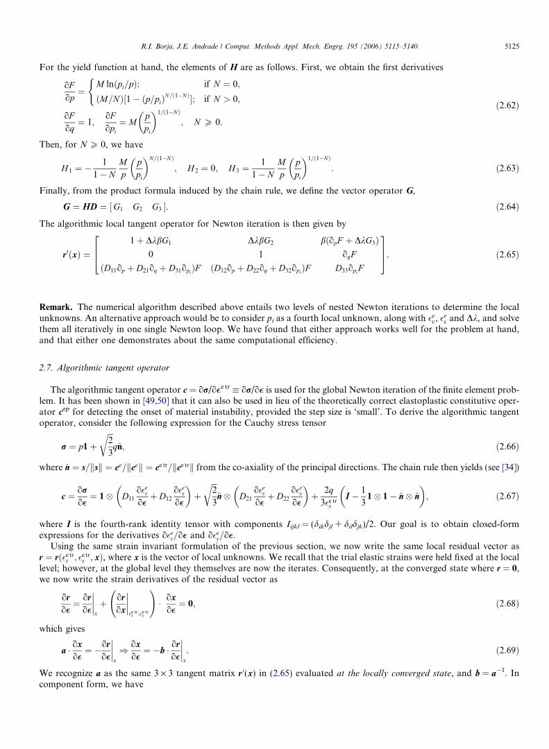
For the yield function at hand, the elements of H are as follows. First, we obtain the first derivatives
oFop¼
M lnðpi=pÞ; if N ¼ 0;
ðM=NÞ½1� ðp=piÞN=ð1�NÞ�; if N > 0;
(oFoq¼ 1;
oFopi
¼ Mppi
� �1=ð1�NÞ
; N P 0.
ð2:62Þ
Then, for N P 0, we have
H 1 ¼ �1
1� NMp
ppi
� �N=ð1�NÞ
; H 2 ¼ 0; H 3 ¼1
1� NMp
ppi
� �1=ð1�NÞ
. ð2:63Þ
Finally, from the product formula induced by the chain rule, we define the vector operator G,
G ¼ HD ¼ G1 G2 G3½ �. ð2:64Þ
The algorithmic local tangent operator for Newton iteration is then given by
r0ðxÞ ¼1þ DkbG1 DkbG2 bðopF þ DkG3Þ
0 1 oqF
ðD11op þ D21oq þ D31opiÞF ðD12op þ D22oq þ D32opi
ÞF D33opiF
264375. ð2:65Þ
Remark. The numerical algorithm described above entails two levels of nested Newton iterations to determine the localunknowns. An alternative approach would be to consider pi as a fourth local unknown, along with �e
v, �es and Dk, and solve
them all iteratively in one single Newton loop. We have found that either approach works well for the problem at hand,and that either one demonstrates about the same computational efficiency.
2.7. Algorithmic tangent operator
The algorithmic tangent operator c = or/o�e tr or/o� is used for the global Newton iteration of the finite element prob-lem. It has been shown in [49,50] that it can also be used in lieu of the theoretically correct elastoplastic constitutive oper-ator cep for detecting the onset of material instability, provided the step size is ‘small’. To derive the algorithmic tangentoperator, consider the following expression for the Cauchy stress tensor
r ¼ p1þffiffiffi2
3
rqn; ð2:66Þ
where n ¼ s=ksk ¼ ee=keek ¼ ee tr=kee trk from the co-axiality of the principal directions. The chain rule then yields (see [34])
c ¼ or
o�¼ 1� D11
o�ev
o�þ D12
o�es
o�
� �þ
ffiffiffi2
3
rn� D21
o�ev
o�þ D22
o�es
o�
� �þ 2q
3�e trs
I � 1
31� 1� n� n
� �; ð2:67Þ
where I is the fourth-rank identity tensor with components Iijkl = (dikdjl + dildjk)/2. Our goal is to obtain closed-formexpressions for the derivatives o�e
v=o� and o�es=o�.
Using the same strain invariant formulation of the previous section, we now write the same local residual vector asr ¼ rð�e tr
v ; �e trs ; xÞ, where x is the vector of local unknowns. We recall that the trial elastic strains were held fixed at the local
level; however, at the global level they themselves are now the iterates. Consequently, at the converged state where r = 0,we now write the strain derivatives of the residual vector as
or
o�¼ or
o�
x
þ or
ox
�e tr
v ;�e trs
!� ox
o�¼ 0; ð2:68Þ
which gives
a � ox
o�¼ �or
o�
x
) ox
o�¼ �b � or
o�
x
. ð2:69Þ
We recognize a as the same 3 · 3 tangent matrix r 0(x) in (2.65) evaluated at the locally converged state, and b = a�1. Incomponent form, we have
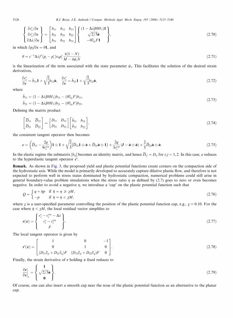
5126 R.I. Borja, J.E. Andrade / Comput. Methods Appl. Mech. Engrg. 195 (2006) 5115–5140
o�ev=o�
o�es=o�
oDk=o�
8><>:9>=>; ¼
b11 b12 b13
b21 b22 b23
b31 b32 b33
264375 ð1� DkbhH 3Þ1ffiffiffiffiffiffiffiffi
2=3p
n
�hopiF 1
8><>:9>=>;; ð2:70Þ
in which opi/o� = h1, and
h ¼ c�1Dkf 0ðpi � p�i Þv0p�i�að1� NÞ
M � �awiNð2:71Þ
is the linearization of the term associated with the state parameter wi. This facilitates the solution of the desired strainderivatives,
o�ev
o�¼ ~b111þ
ffiffiffi2
3
rb12n;
o�es
o�¼ ~b211þ
ffiffiffi2
3
rb22n; ð2:72Þ
where
~b11 ¼ ð1� DkbhH 3Þb11 � ðhopiF Þb13;
~b21 ¼ ð1� DkbhH 3Þb21 � ðhopiF Þb23.
ð2:73Þ
Defining the matrix product
D11 D12
D21 D22
" #¼
D11 D12
D21 D22
� � ~b11 b12
~b21 b22
" #; ð2:74Þ
the consistent tangent operator then becomes
c ¼ D11 �2q
9�e trs
� �1� 1þ
ffiffiffi2
3
rD121� nþ D21n� 1� �
þ 2q3�e tr
s
ðI � n� nÞ þ 2
3D22n� n. ð2:75Þ
In the elastic regime the submatrix [bij] becomes an identity matrix, and hence Dij ¼ Dij for i, j = 1,2. In this case, c reducesto the hyperelastic tangent operator ce.
Remark. As shown in Fig. 3, the proposed yield and plastic potential functions create corners on the compaction side ofthe hydrostatic axis. While the model is primarily developed to accurately capture dilative plastic flow, and therefore is notexpected to perform well in stress states dominated by hydrostatic compaction, numerical problems could still arise ingeneral boundary-value problem simulations when the stress ratio g as defined by (2.7) goes to zero or even becomesnegative. In order to avoid a negative g, we introduce a ‘cap’ on the plastic potential function such that
Q ¼qþ �gp if �g ¼ g P vM ;
�p if �g ¼ g < vM ;
ð2:76Þ
where v is a user-specified parameter controlling the position of the plastic potential function cap, e.g., v = 0.10. For thecase where �g < vM , the local residual vector simplifies to
rðxÞ ¼�e
v � �e trv � Dk
�es � �e tr
s
F
8><>:9>=>;. ð2:77Þ
The local tangent operator is given by
r0ðxÞ ¼1 0 �1
0 1 0
ðD11op þ D21oqÞF ðD12op þ D22oqÞF 0
264375. ð2:78Þ
Finally, the strain derivative of r holding x fixed reduces to
or
o�
x
¼1ffiffiffiffiffiffiffiffi
2=3p
n
0
8><>:9>=>;. ð2:79Þ
Of course, one can also insert a smooth cap near the nose of the plastic potential function as an alternative to the planarcap.
R.I. Borja, J.E. Andrade / Comput. Methods Appl. Mech. Engrg. 195 (2006) 5115–5140 5127
3. Finite deformation plasticity; localization of deformation
In the preceding section we have reformulated an infinitesimal rigid-plastic constitutive model for sands to accommo-date non-associated plasticity and hyperelasticity. In this section we further generalize the model to accommodate finitedeformation plasticity. The final model is then used to capture deformation and failure initiation in dense sands, focusingon the effects of uneven void distribution on the local and global responses.
3.1. Entropy inequality
Consider the multiplicative decomposition of deformation gradient for a local material point X [51–53]
FðX ; tÞ ¼ FeðX ; tÞ � FpðX ; tÞ. ð3:1ÞIn the following we shall use as a measure of elastic deformation the contravariant tensor field be reckoned with respect tothe current placement, called the left Cauchy–Green deformation tensor,
be ¼ Fe � Fet. ð3:2ÞAssume then that the free energy is given by
W ¼ WðX ; be; eps Þ. ð3:3Þ
As in the infinitesimal model, we investigate conditions under which we could isolate an elastic stored energy function fromthe above free energy function.
For the purely mechanical theory the local dissipation function takes the form
D ¼ s : d � dWðX ; be; eps Þ
dtP 0; ð3:4Þ
where s = Jr is the symmetric Kirchhoff stress tensor, J = det (F), d = sym (l) is the rate of deformation tensor, and l is thespatial velocity gradient. Using the chain rule and invoking the standard Coleman relations yields the constitutive equation[54]
s ¼ 2oWðX ; be; ep
s Þobe � be; ð3:5Þ
along with the reduced dissipation inequality
D ¼ s : dp � pi _eps P 0; ð3:6Þ
where d p is the plastic component of the rate of deformation,
dp ¼ sym ðlpÞ; lp :¼ Fe � Lp � Fe�1; Lp :¼ _Fp � Fp�1; ð3:7Þand
pi ¼oWðX ; be; ep
s Þoep
sð3:8Þ
is a stress-like plastic internal variable equivalent to pi of the infinitesimal theory.We assume that pi evolves in the same way as pi, i.e.,
� _pi ¼ /ðpi � p�i Þ_eps ; ð3:9Þ
where p�i depends not only on pi but also on be. Integrating (3.9) gives
pi ¼ pi0 �Z ep
s
eps0
/ðpi � p�i Þdeps . ð3:10Þ
Integrating once more, we get
WðX ; be; eps Þ ¼
Z eps
eps0
pi0 deps �
Z eps
eps0
Z eps
eps0
/ðpi � p�i Þdeps dep
s þWeðX ; beÞ þW0; ð3:11Þ
where We(X,be) is the elastic stored energy function. Finally, using the constitutive Eq. (3.5) once again, we get
s ¼ 2oWeðX ; beÞ
obe þZ ep
s
eps0
Z eps
eps0
/0ðpi � p�i Þop�iobe dep
s deps|fflfflfflfflfflfflfflfflfflfflfflfflfflfflfflfflfflfflfflfflfflfflfflfflfflfflffl{zfflfflfflfflfflfflfflfflfflfflfflfflfflfflfflfflfflfflfflfflfflfflfflfflfflfflffl}
OðDep2s Þ
266664377775 � be. ð3:12Þ
5128 R.I. Borja, J.E. Andrade / Comput. Methods Appl. Mech. Engrg. 195 (2006) 5115–5140
The second-order terms in (3.12) can be ignored at the initial stage of loading when Deps is small, thus leaving the Kirchhoff
stress varying with the elastic stored energy function alone. When Deps is large, /ðpi � p�i Þ vanishes at critical state, and so
the elastic and plastic parts of the free energy uncouple. In both cases the stresses can be expressed in terms of the elasticstored energy function alone, i.e.,
s ¼ 2oWeðX ; beÞ
obe � be. ð3:13Þ
Once again, the perfectly plastic behavior at critical state is a key feature of the model that allows for the uncoupling of thefree energy.
3.2. Finite deformation plasticity model
Consider the stress invariants
p ¼ 1
3trs; q ¼
ffiffiffi3
2
rknk; n ¼ s� p1. ð3:14Þ
Then, as in the infinitesimal theory the yield function can be defined as
F ¼ qþ gp 6 0; ð3:15Þ
where
g ¼M ½1þ lnðpi=pÞ� if N ¼ 0;
ðM=NÞ½1� ð1� NÞðp=piÞN=ð1�NÞ� if N > 0.
(ð3:16Þ
The material parameters M and N are similar in meaning to those of the infinitesimal theory, although their values shouldnow be calibrated in the finite deformation regime. The flow rule may be written as before,
dp ¼ _kq; q ¼ b3
oFop
1þffiffiffi3
2
roFoq
n; n ¼ n=knk; ð3:17Þ
where b 6 1 is the non-associativity parameter. We postulate a similar hardening law in Kirchhoff stress space given by(3.9), with
sgn ½/ðpi � p�i Þ� ¼ sgn H ð3:18Þto capture either a hardening or softening response depending on the position of the state point relative to the limit hard-ening dilatancy. Box 3 then summarizes the rate equations for the finite deformation plasticity model.
The model summarized in Box 3 has some noteworthy features. First, the formulation assumes that the plastic spin xp iszero (see [55] for some discussions on the significance of the plastic spin). Second, the fourth-order spatial elastic tangentoperator ae can be determined from the expression
ae ¼ ce þ s� 1þ s� 1; ð3:19Þ
where (s � 1)ijkl = sjldik, (s � 1)ijkl = sildjk, and ce is a spatial tangential elasticity tensor obtained from the push-forward ofall the indices of the second tangential elasticity tensor defined in [53].
Box 3. Summary of rate equations for plasticity model for sands, finite deformation version
1. Velocity gradient: l = l e + l p.2. Hyperelastic rate equation: _s ¼ ae : le.3. Flow rule: dp ¼ sym ðlpÞ ¼ _kq; xp ¼ skw ðlpÞ ¼ 0.4. State parameter: _wi ¼ _vþ ~k _pi=pi.5. Hardening law: � _pi ¼ /ðpi � p�i Þ _k.6. Consistency condition: f : _s� H _k ¼ 0, f = oF/os.7. Kuhn–Tucker conditions: _k P 0, F 6 0, _kF ¼ 0.
Finally, the specific volume varies according to the kinematical relation
v ¼ Jv0 ) _v ¼ _Jv0 ¼ Jv0tr ðlÞ ¼ v tr ðlÞ. ð3:20Þ
R.I. Borja, J.E. Andrade / Comput. Methods Appl. Mech. Engrg. 195 (2006) 5115–5140 5129
Thus, just as in the infinitesimal theory where the rate equations may be viewed as driven by the strain rate _�, the rate equa-tions shown in Box 3 may be viewed as driven by the spatial velocity gradient l.
3.3. Numerical implementation
For the problem at hand we employ a standard elastic predictor-plastic corrector algorithm based on the productformula for be, as summarized in Box 4. Let
ben ¼ Fe
n � Fetn . ð3:21Þ
Suppressing plastic flow, the trial elastic predictor for be is
be tr be trnþ1 ¼ f nþ1 � be
n � ftnþ1; f nþ1 ¼
oxnþ1
oxn. ð3:22Þ
The plastic corrector emanates from the exponential approximation
be ¼ expð�2DkqÞ � be tr; q qnþ1 ¼oQos
. ð3:23Þ
From the co-axiality of plastic flow, the principal directions of q and s coincide.
Box 4. Return mapping algorithm for plasticity model for sands, finite deformation version
1. Elastic deformation predictor: be tr ¼ f nþ1 � ben � f
tnþ1.
2. Elastic stress predictor: str ¼ 2ðoWe=obe trÞ � be tr; ptri ¼ pi;n.
3. Check if yielding: F ðptr; qtr; ptri ÞP 0?
No, set be ¼ be tr; s ¼ str; pi ¼ ptri and exit.
4. Yes, initialize Dk = 0 and iterate for Dk (steps 5–8).5. Spectral decomposition: be tr ¼
P3A¼1ðk
e trA Þ
2mtrðAÞ.
6. Plastic corrector in principal logarithmic stretches: eeA ¼ lnðke
AÞ, ee trA ¼ lnðke tr
A Þ,ee
A ¼ ee trA � DkqA, sA ¼ oWe=oee
A; A ¼ 1; 2; 3.7. Update plastic internal variable pi:
(a) Total deformation gradient: F = fn+1 Æ Fn.(b) Specific volume: v = det (F)v0 = Jv0.(c) Initialize pi = pi,n and iterate for pi (Steps 7d–f).
(d) State parameter: wi ¼ v� vc0 þ ~k lnð�piÞ.(e) Limit hardening plastic variable:
p�i ¼ p expð�awi=MÞ if N ¼ N ¼ 0;
ð1� �awiN=MÞðN�1Þ=N if 0 6 N 6 N 6¼ 0.
((f) Plastic internal variable: pi ¼ pi;n � /ðpi � p�i ÞDk.
8. Discrete consistency condition: F(p,q,pi) = 0.9. Spectral resolution: be ¼
P3A¼1ðk
eAÞ
2mtrðAÞ.
Next we obtain a spectral decomposition of be,
be ¼X3
A¼1
ðkeAÞ
2mðAÞ; mðAÞ ¼ nðAÞ � nðAÞ; ð3:24Þ
where keA are the elastic principal stretches, n(A) are the unit principal directions, and m(A) are the spectral directions. The
corresponding elastic logarithmic stretches are
eeA ¼ lnðke
AÞ; A ¼ 1; 2; 3. ð3:25ÞFrom material frame indifference We(X,be) only varies with ee
A, and so we can write We ¼ WeðX ; ee1; e
e2; e
e2Þ, which gives
oWe
obe ¼1
2
X3
A¼1
1
ðkeAÞ
2
oWe
oeeA
mðAÞ. ð3:26Þ
5130 R.I. Borja, J.E. Andrade / Comput. Methods Appl. Mech. Engrg. 195 (2006) 5115–5140
The elastic constitutive equation then writes
s ¼ 2oWe
obe � be ¼X3
A¼1
sAmðAÞ; sA ¼oWe
oeeA
; ð3:27Þ
implying that the spectral directions of s and be also coincide. Thus, be and q are also co-axial, and for (3.23) to hold, be andbe tr must also be co-axial, i.e.,
mðAÞ ¼ mtrðAÞ. ð3:28ÞThis allows the plastic corrector phase to take place along the principal axes, as shown in Box 4.
Alternatively, we can utilize the algorithm developed for the infinitesimal theory by working on the invariant space ofthe logarithmic elastic stretch tensor. Let
eev ¼ ee
1 þ ee2 þ ee
3; ees ¼
1
3
ffiffiffiffiffiffiffiffiffiffiffiffiffiffiffiffiffiffiffiffiffiffiffiffiffiffiffiffiffiffiffiffiffiffiffiffiffiffiffiffiffiffiffiffiffiffiffiffiffiffiffiffiffiffiffiffiffiffiffiffiffiffiffiffiffiffiffiffiffiffiffiffiffi2½ðee
1 � ee2Þ
2 þ ðee1 � ee
3Þ2 þ ðee
2 � ee3Þ
2�q
ð3:29Þ
denote the first two invariants of the logarithmic elastic stretch tensor (similar definitions may be made for ee trv and ee tr
s ),and
p ¼ 1
3ðs1 þ s2 þ s3Þ; q ¼
ffiffiffiffiffiffiffiffiffiffiffiffiffiffiffiffiffiffiffiffiffiffiffiffiffiffiffiffiffiffiffiffiffiffiffiffiffiffiffiffiffiffiffiffiffiffiffiffiffiffiffiffiffiffiffiffiffiffiffiffiffiffiffiffiffiffiffiffiffiffiffiffiffiffiffiffiffi½ðs1 � s2Þ2 þ ðs1 � s3Þ2 þ ðs2 � s3Þ2�=2
qð3:30Þ
denote the first two invariants of the Kirchhoff stress tensor. If we take the functional relationships p ¼ pðeev; e
esÞ,
q ¼ qðeev; e
esÞ, and pi ¼ piðee
v; ees ;DkÞ as before, using the same elastic stored energy function but now expressed in terms
of the logarithmic principal elastic stretches, then the local residual vector writes
r ¼ rðxÞ ¼ee
v � ee trv þ DkbopF
ees � ee tr
s þ DkoqF
F
8><>:9>=>;; x ¼
eev
ees
Dk
8><>:9>=>;. ð3:31Þ
In this case, the local Jacobian r 0(x) takes a form identical to that developed for the infinitesimal theory, see (2.65).Comparing Boxes 2 and 4, we see that the algorithm for finite deformation plasticity differs from the infinitesimal ver-
sion only through a few additional steps entailed for the spectral decomposition and resolution of the deformation andstress tensors. Construction of be from the spectral values requires two steps. The first involves resolution of the principalelastic logarithmic stretches from the first two invariants calculated from return mapping,
eeA ¼
1
3ee
vdA þffiffiffi3
2
ree
s nA; nA ¼ffiffiffi2
3
ree tr
A � ðee trv =3ÞdA
ee trs
; ð3:32Þ
where dA = 1 for A = 1,2,3. The above transformation entails scaling the deviatoric component of the predictor tensor bythe factor ee
s=ee trs and adding the volumetric component. The second step involves a spectral resolution from the principal
elastic logarithmic strains (cf. (3.24))
be ¼X3
A¼1
expð2eeAÞmtrðAÞ. ð3:33Þ
The next section demonstrates that a closed-form consistent tangent operator is available for the above algorithm.
3.4. Algorithmic tangent operator
For simplicity, we restrict to a quasi-static problem whose weak form of the linear momentum balance over an initialvolume B with surface oB readsZ
B
ðGRADg : P � q0g � GÞdV �Z
oBtg � t dA ¼ 0; ð3:34Þ
where q0G is the reference body force vector, t = P Æ n is the nominal traction vector on oBt � oB, n is the unit vector onoBt, g is the weighting function,
P ¼ s � F�t ð3:35Þis the non-symmetric first Piola–Kirchhoff stress tensor, and GRAD is the gradient operator evaluated with respect to thereference configuration. We recall the internal virtual work
R.I. Borja, J.E. Andrade / Comput. Methods Appl. Mech. Engrg. 195 (2006) 5115–5140 5131
W eINT ¼
ZBe
GRADg : P dV ¼ZBe
gradg : sdV ð3:36Þ
for any Be � B, where grad is the gradient operator evaluated with respect to the current configuration. The first variationgives [56]
dW eINT ¼
ZBe
gradg : a : graddudV ; ð3:37Þ
where u is the displacement field, and
a ¼ a� s� 1; ds ¼ a : graddu. ð3:38ÞEvaluation of a thus requires determination of the algorithmic tangent operator a.
We also recall the following spectral representation of the algorithmic tangent operator a [56]
a ¼X3
A¼1
X3
B¼1
aABmðAÞ �mðBÞ þX3
A¼1
XB 6¼A
sB � sA
ke tr2B � ke tr2
A
ke tr2B mðABÞ �mðABÞ þ ke tr2
A mðABÞ �mðBAÞ� �; ð3:39Þ
where m(AB) = n(A) � n(B), A 5 B. The coefficients aAB are elements of the consistent tangent operator obtained from a re-turn mapping in principal axes, and is formally defined as
aAB ¼osA
oee trB
osA
oeB; A;B ¼ 1; 2; 3. ð3:40Þ
The values of these coefficients are specific to the constitutive model in question, as well as dependent on the numericalintegration algorithm utilized for the model. For the present critical state plasticity theory aAB is evaluated as follows.
The expression for a principal Kirchhoff stress is
sA ¼ pdA þffiffiffi2
3
rqnA; A ¼ 1; 2; 3. ð3:41Þ
Differentiating with respect to a principal logarithmic strain gives
aAB ¼osA
oeB¼ dA D11
oeev
oeBþ D12
oees
oeB
� �þ
ffiffiffi2
3
rnA D21
oeev
oeBþ D22
oees
oeB
� �þ 2q
3ee trs
dAB �1
3dAdB � nAnB
� �; A;B ¼ 1; 2; 3; ð3:42Þ
where dAB is the Kronecker delta. The coefficients D11, D22, and D21 are identical in form to those shown in (2.52) exceptthat the strain invariants now take on logarithmic definitions. As in the infinitesimal theory, we obtain the unknown strainderivatives above from the local residual vector, whose own derivatives write
orA
oeB¼ orA
oeB
x
þX3
C¼1
orA
oxC
ee tr
v ;ee trs|fflfflfflfflfflffl{zfflfflfflfflfflffl}
�aAC
oxC
oeB¼ 0; A;B ¼ 1; 2; 3; ð3:43Þ
where the matrix ½�aAB� corresponds to the same algorithmic local tangent operator given in (2.65). Letting [bAB] denote theinverse of ½�aAB�, we can then solve
oxA
oeB¼ �
X3
C¼1
bACorC
oeB
x
; A;B ¼ 1; 2; 3. ð3:44Þ
This latter equation provides the desired strain derivatives,
oeev=oeA
oees=oeA
oDk=oeA
8<:9=; ¼
b11 b12 b13
b21 b22 b23
b31 b32 b33
24 35 ð1� DkbhH 3ÞdAffiffiffiffiffiffiffiffi2=3
pnA
�hopi F dA
8<:9=;; A ¼ 1; 2; 3; ð3:45Þ
where
h ¼ c�1Dk/0ðpi � p�i Þvp�i�að1� NÞ
M � �awiN;
c ¼ 1þ /0ðpi � p�i ÞDk 1�~k�að1� NÞM � �awiN
p�ipi
� �" #.
ð3:46Þ
5132 R.I. Borja, J.E. Andrade / Comput. Methods Appl. Mech. Engrg. 195 (2006) 5115–5140
Note that the finite deformation expression for h utilizes the current value of the specific volume v whereas the infinitesimalversion uses the initial value v0 (cf. (2.71)). Inserting the expressions for oee
v=oeA and oees=oeA back in (3.42) yields the closed-
form solution for aAB, which takes an identical form to (2.75):
aAB ¼ D11 �2q
9ee trs
� �dAdB þ
ffiffiffi2
3
rD12dAnB þ D21nAdB
� �þ 2q
3ee trs
ðdAB � nAnBÞ þ2
3D22nAnB; A;B ¼ 1; 2; 3. ð3:47Þ
See (2.72)–(2.74) for specific expressions for the coefficients Dij.
3.5. Localization condition
Following [56,57], we summarize the following alternative (and equivalent) expressions for the localization conditioninto planar bands. We denote the continuum elastoplastic counterpart of the algorithmic tensor a by
aep ¼X3
A¼1
X3
B¼1
aepABmðAÞ �mðBÞ þ
X3
A¼1
XB6¼A
sB � sA
ke2B � ke2
A
ke2B mðABÞ �mðABÞ þ ke2
A mðABÞ �mðBAÞ� �; ð3:48Þ
where aepAB is the continuum elastoplastic tangent stiffness matrix in principal axes. (Note, this formula appears in [46,49,50]
with a factor ‘‘1/2’’ before the spin-term summations, a typographical error.) Then,
aep ¼ aep � s� 1 ð3:49Þdefines the continuum counterpart of the fourth-order tensor a in (3.38).
Alternatively, we denote the constitutive elastoplastic material tensor cep by the expression [54]
cep ¼X3
A¼1
X3
B¼1
aepABmðAÞ �mðBÞ þ
X3
A¼1
sAxðAÞ; ð3:50Þ
in which
xðAÞ ¼ 2½Ib � be � be þ I3b�1A ð1� 1� IÞ þ bAðbe �mðAÞ þmðAÞ � beÞ
� I3b�1A ð1�mðAÞ þmðAÞ � 1Þ þ wmðAÞ �mðAÞ�=DA; ð3:51Þ
where bA is the Ath principal value of be, I1 and I3 are the first and third invariants of be,
Ib ¼ ðbe � be þ be � beÞ=2; w ¼ I1bA þ I3b�1A � 4b2
A; ð3:52Þand
DA :¼ 2b2A � I1bA þ I3b�1
A . ð3:53ÞNote that cep
ijkl ¼ 2F iAF jBF kCF lDCepABCD is the spatial push-forward of the first tangential elastoplastic tensor Cep [53]. Then,
aep ¼ cep þ s� 1 ð3:54Þdefines an alternative expression to (3.49).
Using aep from either (3.49) or (3.54), we can evaluate the elements of the Eulerian elastoplastic acoustic tensor a as
aij ¼ nkaepikjlnl; ð3:55Þ
where nk and nl are elements of the unit normal vector n to a potential deformation band reckoned with respect to the cur-rent configuration. Defining the localization function as
F ¼ inf jnðdet aÞ; ð3:56Þwe can then infer the inception of a deformation band from the initial vanishing of F. Though theoretically one needs touse the constitutive operators aep or cep to obtain the acoustic tensor a, the algorithmic tangent tensors are equally accept-able for bifurcation analyses for small step sizes [50].
4. Numerical simulations
We present two numerical examples demonstrating the meso-scale modeling technique. To highlight the triggering ofstrain localization via imposed material inhomogeneity, we only considered regular specimens (either rectangular or cubi-cal) along with boundary conditions favoring the development of homogeneous deformation (a pin to arrest rigid bodymodes and vertical rollers at the top and bottom ends of the specimen). A common technique of perturbing the initialcondition is to prescribe a weak element; however, this is unrealistic and arbitrary. In the following simulations we have
R.I. Borja, J.E. Andrade / Comput. Methods Appl. Mech. Engrg. 195 (2006) 5115–5140 5133
perturbed the initial condition by prescribing a spatially varying specific volume (or void ratio) consisting of horizontallayers of relatively homogeneous density but with some variation in the vertical direction. This resulted in vein-like soilstructures in the density field closely resembling that shown in the photograph of Fig. 1 and mimicked the placement ofsand with a common laboratory technique called pluviation. The specific volume fields were assumed to range from1.60 to 1.70, with a mean value of 1.63. These values were chosen such that all points remained on the dense side ofthe CSL (wi < 0).
4.1. Plane strain simulation
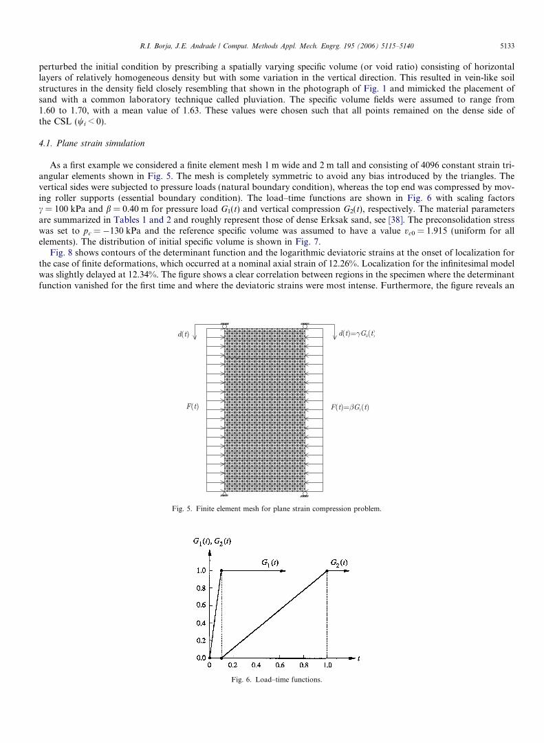
As a first example we considered a finite element mesh 1 m wide and 2 m tall and consisting of 4096 constant strain tri-angular elements shown in Fig. 5. The mesh is completely symmetric to avoid any bias introduced by the triangles. Thevertical sides were subjected to pressure loads (natural boundary condition), whereas the top end was compressed by mov-ing roller supports (essential boundary condition). The load–time functions are shown in Fig. 6 with scaling factorsc = 100 kPa and b = 0.40 m for pressure load G1(t) and vertical compression G2(t), respectively. The material parametersare summarized in Tables 1 and 2 and roughly represent those of dense Erksak sand, see [38]. The preconsolidation stresswas set to pc = �130 kPa and the reference specific volume was assumed to have a value vc0 = 1.915 (uniform for allelements). The distribution of initial specific volume is shown in Fig. 7.
Fig. 8 shows contours of the determinant function and the logarithmic deviatoric strains at the onset of localization forthe case of finite deformations, which occurred at a nominal axial strain of 12.26%. Localization for the infinitesimal modelwas slightly delayed at 12.34%. The figure shows a clear correlation between regions in the specimen where the determinantfunction vanished for the first time and where the deviatoric strains were most intense. Furthermore, the figure reveals an
Fig. 5. Finite element mesh for plane strain compression problem.
Fig. 6. Load–time functions.
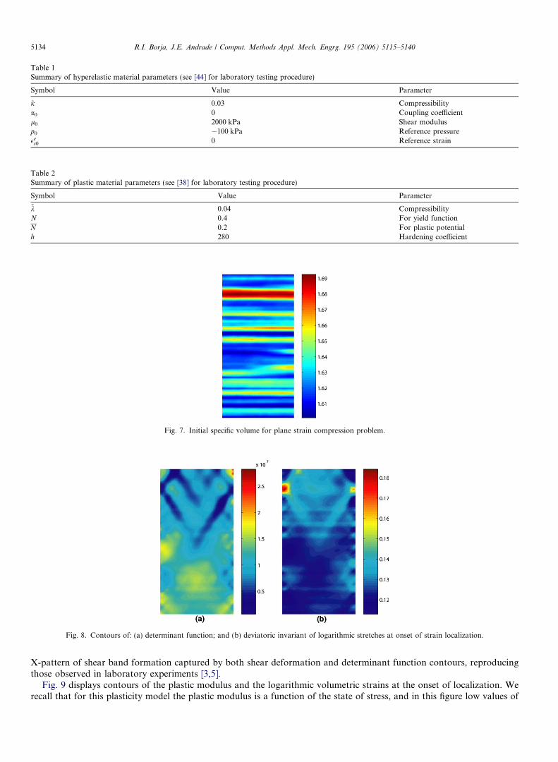
Table 2Summary of plastic material parameters (see [38] for laboratory testing procedure)
Symbol Value Parameter
~k 0.04 CompressibilityN 0.4 For yield functionN 0.2 For plastic potentialh 280 Hardening coefficient
Fig. 7. Initial specific volume for plane strain compression problem.
Table 1Summary of hyperelastic material parameters (see [44] for laboratory testing procedure)
Symbol Value Parameter
~j 0.03 Compressibilitya0 0 Coupling coefficientl0 2000 kPa Shear modulusp0 �100 kPa Reference pressure�e
v0 0 Reference strain
Fig. 8. Contours of: (a) determinant function; and (b) deviatoric invariant of logarithmic stretches at onset of strain localization.
5134 R.I. Borja, J.E. Andrade / Comput. Methods Appl. Mech. Engrg. 195 (2006) 5115–5140
X-pattern of shear band formation captured by both shear deformation and determinant function contours, reproducingthose observed in laboratory experiments [3,5].
Fig. 9 displays contours of the plastic modulus and the logarithmic volumetric strains at the onset of localization. Werecall that for this plasticity model the plastic modulus is a function of the state of stress, and in this figure low values of
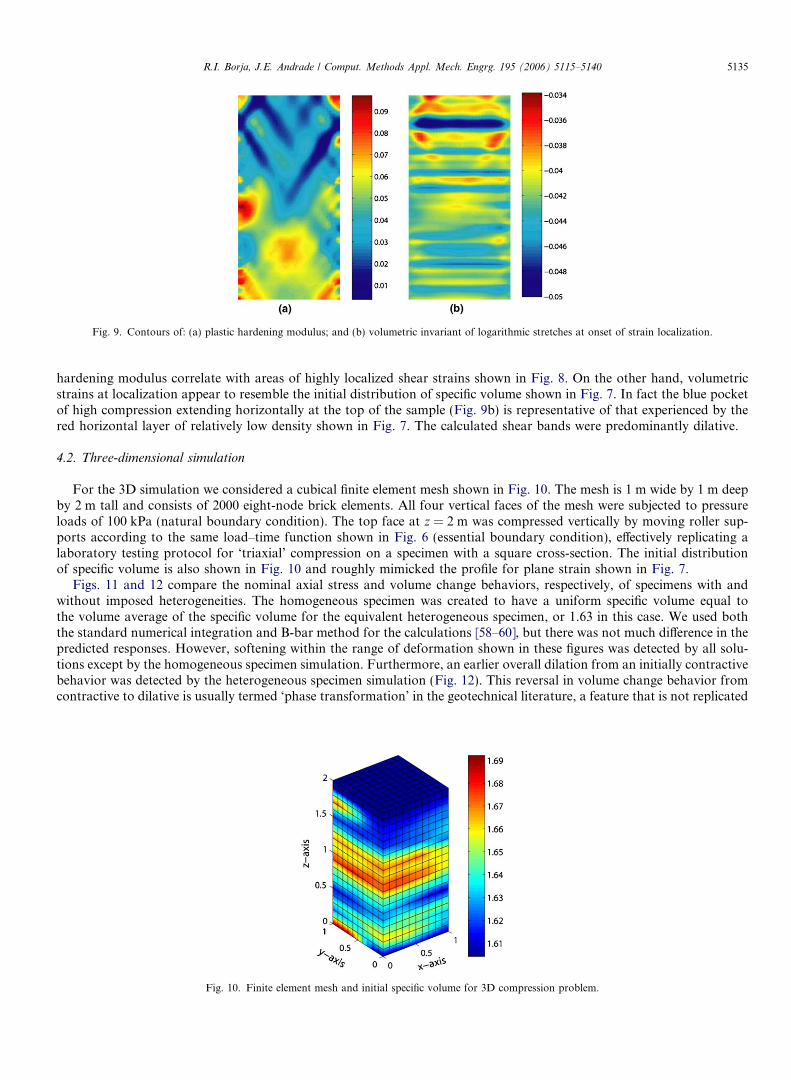
Fig. 9. Contours of: (a) plastic hardening modulus; and (b) volumetric invariant of logarithmic stretches at onset of strain localization.
R.I. Borja, J.E. Andrade / Comput. Methods Appl. Mech. Engrg. 195 (2006) 5115–5140 5135
hardening modulus correlate with areas of highly localized shear strains shown in Fig. 8. On the other hand, volumetricstrains at localization appear to resemble the initial distribution of specific volume shown in Fig. 7. In fact the blue pocketof high compression extending horizontally at the top of the sample (Fig. 9b) is representative of that experienced by thered horizontal layer of relatively low density shown in Fig. 7. The calculated shear bands were predominantly dilative.
4.2. Three-dimensional simulation
For the 3D simulation we considered a cubical finite element mesh shown in Fig. 10. The mesh is 1 m wide by 1 m deepby 2 m tall and consists of 2000 eight-node brick elements. All four vertical faces of the mesh were subjected to pressureloads of 100 kPa (natural boundary condition). The top face at z = 2 m was compressed vertically by moving roller sup-ports according to the same load–time function shown in Fig. 6 (essential boundary condition), effectively replicating alaboratory testing protocol for ‘triaxial’ compression on a specimen with a square cross-section. The initial distributionof specific volume is also shown in Fig. 10 and roughly mimicked the profile for plane strain shown in Fig. 7.
Figs. 11 and 12 compare the nominal axial stress and volume change behaviors, respectively, of specimens with andwithout imposed heterogeneities. The homogeneous specimen was created to have a uniform specific volume equal tothe volume average of the specific volume for the equivalent heterogeneous specimen, or 1.63 in this case. We used boththe standard numerical integration and B-bar method for the calculations [58–60], but there was not much difference in thepredicted responses. However, softening within the range of deformation shown in these figures was detected by all solu-tions except by the homogeneous specimen simulation. Furthermore, an earlier overall dilation from an initially contractivebehavior was detected by the heterogeneous specimen simulation (Fig. 12). This reversal in volume change behavior fromcontractive to dilative is usually termed ‘phase transformation’ in the geotechnical literature, a feature that is not replicated
Fig. 10. Finite element mesh and initial specific volume for 3D compression problem.
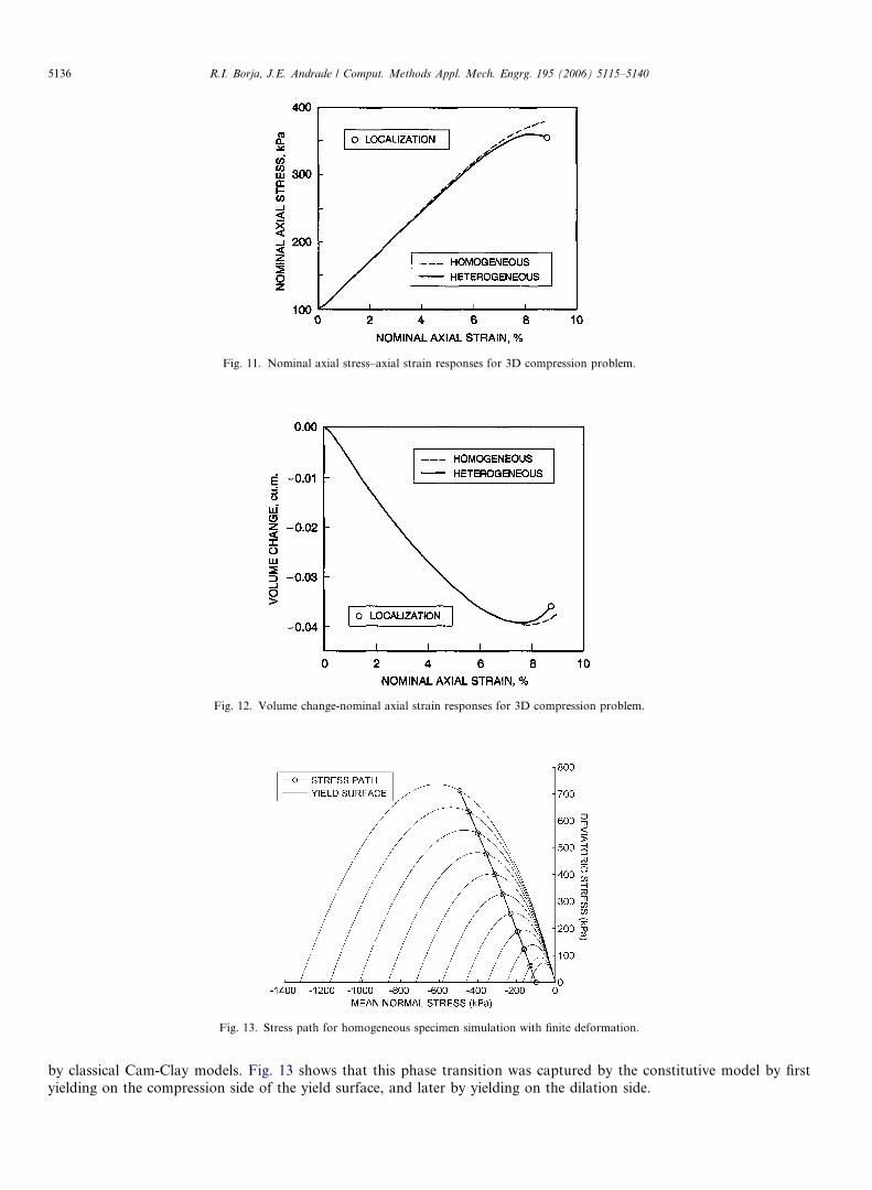
Fig. 12. Volume change-nominal axial strain responses for 3D compression problem.
Fig. 11. Nominal axial stress–axial strain responses for 3D compression problem.
Fig. 13. Stress path for homogeneous specimen simulation with finite deformation.
5136 R.I. Borja, J.E. Andrade / Comput. Methods Appl. Mech. Engrg. 195 (2006) 5115–5140
by classical Cam-Clay models. Fig. 13 shows that this phase transition was captured by the constitutive model by firstyielding on the compression side of the yield surface, and later by yielding on the dilation side.
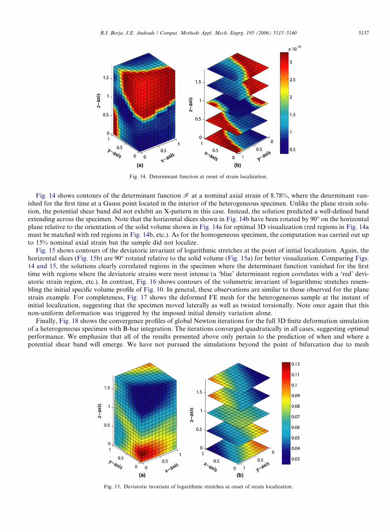
Fig. 14. Determinant function at onset of strain localization.
R.I. Borja, J.E. Andrade / Comput. Methods Appl. Mech. Engrg. 195 (2006) 5115–5140 5137
Fig. 14 shows contours of the determinant function F at a nominal axial strain of 8.78%, where the determinant van-ished for the first time at a Gauss point located in the interior of the heterogeneous specimen. Unlike the plane strain solu-tion, the potential shear band did not exhibit an X-pattern in this case. Instead, the solution predicted a well-defined bandextending across the specimen. Note that the horizontal slices shown in Fig. 14b have been rotated by 90� on the horizontalplane relative to the orientation of the solid volume shown in Fig. 14a for optimal 3D visualization (red regions in Fig. 14amust be matched with red regions in Fig. 14b, etc.). As for the homogeneous specimen, the computation was carried out upto 15% nominal axial strain but the sample did not localize.
Fig. 15 shows contours of the deviatoric invariant of logarithmic stretches at the point of initial localization. Again, thehorizontal slices (Fig. 15b) are 90� rotated relative to the solid volume (Fig. 15a) for better visualization. Comparing Figs.14 and 15, the solutions clearly correlated regions in the specimen where the determinant function vanished for the firsttime with regions where the deviatoric strains were most intense (a ‘blue’ determinant region correlates with a ‘red’ devi-atoric strain region, etc.). In contrast, Fig. 16 shows contours of the volumetric invariant of logarithmic stretches resem-bling the initial specific volume profile of Fig. 10. In general, these observations are similar to those observed for the planestrain example. For completeness, Fig. 17 shows the deformed FE mesh for the heterogeneous sample at the instant ofinitial localization, suggesting that the specimen moved laterally as well as twisted torsionally. Note once again that thisnon-uniform deformation was triggered by the imposed initial density variation alone.
Finally, Fig. 18 shows the convergence profiles of global Newton iterations for the full 3D finite deformation simulationof a heterogeneous specimen with B-bar integration. The iterations converged quadratically in all cases, suggesting optimalperformance. We emphasize that all of the results presented above only pertain to the prediction of when and where apotential shear band will emerge. We have not pursued the simulations beyond the point of bifurcation due to mesh
Fig. 15. Deviatoric invariant of logarithmic stretches at onset of strain localization.
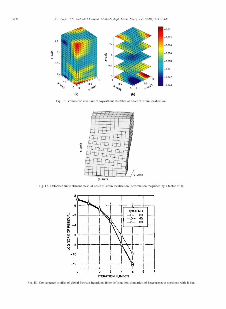
Fig. 16. Volumetric invariant of logarithmic stretches at onset of strain localization.
Fig. 17. Deformed finite element mesh at onset of strain localization (deformation magnified by a factor of 3).
Fig. 18. Convergence profiles of global Newton iterations: finite deformation simulation of heterogeneous specimen with B-bar.
5138 R.I. Borja, J.E. Andrade / Comput. Methods Appl. Mech. Engrg. 195 (2006) 5115–5140
R.I. Borja, J.E. Andrade / Comput. Methods Appl. Mech. Engrg. 195 (2006) 5115–5140 5139
sensitivity issues inherent in rate-independent classical plasticity models in the post-localized regime. A host of regulariza-tion techniques either in the constitutive description or finite element solution are available and should be used to advancethe solution to this regime.
5. Closure
We have presented a meso-scale finite element modeling approach for capturing deformation and strain localization indense granular materials using critical state plasticity theory and nonlinear finite element analysis. This approach has beenmotivated in large part by recent trends in geotechnical laboratory testing allowing accurate quantitative measurement ofthe spatial density variation in discrete granular materials. The meso-scale approach provides a more realistic mathematicalrepresentation of imperfection; hence, it is expected to provide a more thorough capture of the deformation and strainlocalization processes in these materials. Potential extensions of the studies include a three-invariant enhancement ofthe plasticity model and application of the model to unstructured random density fields (in contrast to the structured den-sity fields simulated in this paper). These aspects will be reported upon in a future publication.
Acknowledgements
This work has been supported by National Science Foundation under Grant Nos. CMS-0201317 and CMS-0324674 toStanford University. We thank Professor Jack Baker of Stanford University for his assistance in generating the initial spe-cific volume profiles used in the numerical examples, and Professor Amy Rechenmacher of USC for providing the X-RayCT image shown in Fig. 1. We also thank the two anonymous reviewers for their constructive reviews.
References
[1] K.A. Alshibli, S. Sture, N.C. Costes, M.L. Frank, F.R. Lankton, S.N. Batiste, R.A. Swanson, Assessment of localized deformations in sand usingX-ray computed tomography, Geotech. Test. J. 23 (2000) 274–299.
[2] K.A. Alshibli, S. Sture, Shear band formation in plane strain compression, J. Geotech. Geoenviron. Engrg. 126 (2000) 495–503.[3] K.A. Alshibli, S.N. Batiste, S. Sture, Strain localization in sand: plane strain versus triaxial compression, J. Geotech. Geoenviron. Engrg. 129 (2003)
483–494.[4] J. Desrues, R. Chambon, M. Mokni, F. Mazerolle, Void ratio evolution inside shear bands in triaxial sand specimens studied by computed
tomography, Geotechnique 46 (1996) 527–546.[5] J. Desrues, G. Viggiani, Strain localization in sand: an overview of the experimental results obtained in Grenoble using stereophotogrammetry, Int. J.
Numer. Analyt. Methods Geomech. 28 (2004) 279–321.[6] R.J. Finno, W.W. Harris, M.A. Mooney, Strain localization and undrained steady state of sands, J. Geotech. Engrg. ASCE 122 (1996) 462–473.[7] G. Gudehus, K. Nubel, Evolution of shear bands in sand, Geotechnique 54 (2004) 187–201.[8] A.L. Rechenmacher, R.J. Finno, Digital image correlation to evaluate shear banding in dilative sands, Geotech. Test. J. 27 (2004) 13–22.[9] A.L. Rechenmacher, R.J. Finno, Shear band displacements and void ratio evolution to critical state in dilative sands, in: J.F. Labuz, A. Drescher
(Eds.), Bifurcations & Instabilities in Geomechanics, A.A. Blakema Publishers, Lisse, 2003, pp. 193–206.[10] I. Vardoulakis, M. Goldscheider, G. Gudehus, Formation of shear bands in sand bodies as a bifurcation problem, Int. J. Numer. Analyt. Methods
Geomech. 2 (1978) 99–128.[11] I. Vardoulakis, B. Graf, Calibration of constitutive models for granular materials using data from biaxial experiments, Geotechnique 35 (1985)
299–317.[12] E. Bauer, W. Wu, W. Huang, Influence of an initially transverse isotropy on shear banding in granular materials, in: J.F. Labuz, A. Drescher (Eds.),
Bifurcations & Instabilities in Geomechanics, A.A. Balkema, Lisse, 2003, pp. 161–172.[13] R.I. Borja, T.Y. Lai, Propagation of localization instability under active and passive loading, J. Geotech. Geoenviron. Engrg. ASCE 128 (2002)
64–75.[14] R. Chambon, J.-C. Moullet, Uniqueness studies in boundary value problems involving some second gradient models, Comput. Methods Appl. Mech.
Engrg. 193 (2004) 2771–2796.[15] R. Chambon, D. Caillerie, C. Tamagnini, A strain space gradient plasticity theory for finite strain, Comput. Methods Appl. Mech. Engrg. 193 (2004)
2797–2826.[16] F. Darve, G. Servant, F. Laouafa, H.D.V. Khoa, Failure in geomaterials: continuous and discrete analyses, Comput. Methods Appl. Mech. Engrg.
193 (2004) 3057–3085.[17] R. de Borst, H.-B. Muhlhaus, Gradient-dependent plasticity: formulation and algorithmic aspects, Int. J. Numer. Methods Engrg. 35 (1992) 521–539.[18] A. Gajo, D. Bigoni, D. Muir Wood, Stress induced elastic anisotropy and strain localisation in sand, in: H.-B. Muhlhaus, A. Dyskin, E. Pasternak
(Eds.), Bifurcation and Localisation Theory in Geomechanics, A.A. Balkema, Lisse, 2001, pp. 37–44.[19] S. Kimoto, F. Oka, Y. Higo, Strain localization analysis of elasto-viscoplastic soil considering structural degradation, Comput. Methods Appl. Mech.
Engrg. 193 (2004) 2845–2866.[20] P.A. Klerck, E.J. Sellers, D.R.J. Owen, Discrete fracture in quasi-brittle materials under compressive and tensile stress states, Comput. Methods Appl.
Mech. Engrg. 193 (2004) 3035–3056.[21] B. Muhunthan, O. Alhattamleh, H.M. Zbib, Modeling of localization in granular materials: effect of porosity and particle size, in: J.F. Labuz, A.
Drescher (Eds.), Bifurcations & Instabilities in Geomechanics, A.A. Balkema, Lisse, 2003, pp. 121–131.[22] K. Nubel, W. Huang, A study of localized deformation pattern in granular media, Comput. Methods Appl. Mech. Engrg. 193 (2004) 2719–2743.
5140 R.I. Borja, J.E. Andrade / Comput. Methods Appl. Mech. Engrg. 195 (2006) 5115–5140
[23] E. Onate, J. Rojek, Combination of discrete element and finite element methods for dynamic analysis of geomechanics problems, Comput. MethodsAppl. Mech. Engrg. 193 (2004) 3087–3128.
[24] M. Ortiz, A. Pandolfi, A variational Cam-Clay theory of plasticity, Comput. Methods Appl. Mech. Engrg. 193 (2004) 2645–2666.[25] M.R. Salari, S. Saeb, K.J. Willam, S.J. Patchet, R.C. Carrasco, A coupled elastoplastic damage model for geomaterials, Comput. Methods Appl.
Mech. Engrg. 193 (2004) 2625–2643.[26] J. Tejchman, G. Gudehus, Shearing of a narrow granular layer with polar quantities, Int. J. Numer. Analyt. Methods Geomech. 25 (2001) 1–28.[27] I. Vardoulakis, E. Vairaktaris, E. Papamichos, Subsidence diffusion–convection: I. The direct problem, Comput. Methods Appl. Mech. Engrg. 193
(2004) 2745–2760.[28] R.G. Wan, P.J. Guo, Constitutive modelling of granular materials with focus to microstructure and its effect on strain localization, in: J.F. Labuz, A.
Drescher (Eds.), Bifurcations & Instabilities in Geomechanics, A.A. Balkema, Lisse, 2003, pp. 149–160.[29] Z.Q. Yue, S. Chen, L.G. Tham, Finite element modeling of geomaterials using digital image processing, Comput. Geotech. 30 (2003) 375–397.[30] K.H. Roscoe, J.H. Burland, On the generalized stress–strain behavior of ‘wet’ clay, in: J. Heyman, F.A. Leckie (Eds.), Engineering Plasticity,
Cambridge University Press, Cambridge, 1968, pp. 535–609.[31] A. Schofield, P. Wroth, Critical State Soil Mechanics, McGraw-Hill, New York, 1968.[32] R.I. Borja, S.R. Lee, Cam-Clay plasticity, Part I: Implicit integration of elasto-plastic constitutive relations, Comput. Methods Appl. Mech. Engrg. 78
(1990) 49–72.[33] R.I. Borja, Cam-Clay plasticity, Part II: Implicit integration of constitutive equation based on a nonlinear elastic stress predictor, Comput. Methods
Appl. Mech. Engrg. 88 (1991) 225–240.[34] R.I. Borja, C. Tamagnini, Cam-Clay plasticity, Part III: Extension of the infinitesimal model to include finite strains, Comput. Methods Appl. Mech.
Engrg. 155 (1998) 73–95.[35] D. Peric, M.A. Ayari, Influence of Lode’s angle on the pore pressure generation in soils, Int. J. Plast. 18 (2002) 1039–1059.[36] D. Peric, M.A. Ayari, On the analytical solutions for the three-invariant Cam clay model, Int. J. Plast. 18 (2002) 1061–1082.[37] K. Been, M.G. Jefferies, A state parameter for sands, Geotechnique 35 (1985) 99–112.[38] M.G. Jefferies, Nor-Sand: a simple critical state model for sand, Geotechnique 43 (1993) 91–103.[39] M.T. Manzari, Y.F. Dafalias, A critical state two-surface plasticity model for sands, Geotechnique 47 (1997) 255–272.[40] K. Ishihara, F. Tatsuoka, S. Yasuda, Undrained deformation and liquefaction of sand under cyclic stresses, Soils Found. 15 (1975) 29–44.[41] S.L. Kramer, Geotechnical Earthquake Engineering, Prentice-Hall, New Jersey, 1996.[42] A. Gens, D.M. Potts, Critical state models in computational geomechanics, Eng. Comput. 5 (1988) 178–197.[43] R.J. Jardine, D.M. Potts, A.B. Fourie, J.B. Burland, Studies of the influence of non-linear stress–strain characteristics in soil–structure interaction,
Geotechnique 36 (1986) 377–396.[44] G.T. Houlsby, The use of a variable shear modulus in elastic–plastic models for clays, Comput. Geotech. 1 (1985) 3–13.[45] P.V. Lade, Static instability and liquefaction of loose fine sandy slopes, J. Geotech. Engrg. ASCE 118 (1992) 51–71.[46] R.I. Borja, K.M. Sama, P.F. Sanz, On the numerical integration of three-invariant elastoplastic constitutive models, Comput. Methods Appl. Mech.
Engrg. 192 (2003) 1227–1258.[47] J.C. Simo, T.J.R. Hughes, Computational Inelasticity, Springer-Verlag, New York, NY, 1998.[48] J. Sulem, I. Vardoulakis, E. Papamichos, A. Oulahna, J. Tronvoll, Elasto-plastic modelling of Red Wildmoor sandstone, Mech. Cohes.-Frict. Mater.
4 (1999) 215–245.[49] R.I. Borja, A. Aydin, Computational modeling of deformation bands in granular media, I. Geological and mathematical framework, Comput.
Methods Appl. Mech. Engrg. 193 (2004) 2667–2698.[50] R.I. Borja, Computational modeling of deformation bands in granular media, II. Numerical simulations, Comput. Methods Appl. Mech. Engrg. 193
(2004) 2699–2718.[51] E.H. Lee, Elastic–plastic deformation at finite strains, J. Appl. Mech. (1969) 1–6.[52] L.E. Malvern, Introduction to the Mechanics of a Continuous Medium, Prentice-Hall, Englewood Cliffs, NJ, 1969.[53] J.E. Marsden, T.J.R. Hughes, Mathematical Theory of Elasticity, Dover Publications, New York, NY, 1983.[54] J.C. Simo, Algorithms for static and dynamic multiplicative plasticity that preserve the classical return mapping schemes of the infinitesimal theory,
Comput. Methods Appl. Mech. Engrg. 99 (1992) 61–112.[55] Y.F. Dafalias, Plastic spin: necessity or redundancy? Int. J. Plast. 14 (1998) 909–931.[56] R.I. Borja, Bifurcation of elastoplastic solids to shear band mode at finite strain, Comput. Methods Appl. Mech. Engrg. 191 (2002) 5287–5314.[57] J.W. Rudnicki, J.R. Rice, Conditions for the localization of deformation in pressure-sensitive dilatant materials, J. Mech. Phys. Solids 23 (1975)
371–394.[58] T.J.R. Hughes, The Finite Element Method, Prentice-Hall, Englewood Cliffs, NJ, 1987.[59] J.C. Nagtegaal, D.M. Parks, J.R. Rice, On numerically accurate finite element solutions in the fully plastic range, Comput. Methods Appl. Mech.
Engrg. 4 (1974) 153–177.[60] J.C. Simo, R.L. Taylor, K.S. Pister, Variational and projection methods for the volume constraint in finite deformation elasto-plasticity, Comput.
Methods Appl. Mech. Engrg. 51 (1985) 177–208.