Comparison of very long baseline interferometry,

GPS, and satellite laser ranging height residuals from

ITRF2005 using spectral and correlation methods

X. Collilieux,1 Z. Altamimi,1 D. Coulot,1 J. Ray,2 and P. Sillard3

Received 10 January 2007; revised 20 July 2007; accepted 18 September 2007; published 28 December 2007.

[1] For the first time, the ITRF2005 input data are in the form of time series of stationpositions and Earth orientation parameters, together with full variance-covarianceinformation. The first step of the ITRF2005 analysis consists of rigorously stacking eachtime series to yield a long-term solution per technique. As a by-product, time series ofposition residuals contain the nonlinear motion of points over the Earth’s surface. In thispaper, the height residual time series of very long baseline interferometry (VLBI), GlobalPositioning System (GPS), and satellite laser ranging (SLR) solutions submitted toITRF2005 are compared. We note that the interpretation of the ITRF2005 position residualtime series as observed physical motions at the various stations is delicate due to theinhomogeneous site distribution. We estimate that the network effect may introduce anaveraged scatter of 3 and 2 mm in the VLBI and SLR height residuals, respectively.Although noise levels are different among these three techniques, a common 1.0 cycles peryear (cpy) frequency is clearly detected. The GPS height annual signal exhibits significantregional correlations that are confirmed by VLBI and SLR measurements in somecolocated sites. Significant power near frequencies 2.00, 3.12, and 4.16 cpy is alsodetected in the individual GPS height residuals time series as mentioned by Ray et al.(2007). However, neither VLBI nor SLR show any significant signals at these frequenciesfor colocated sites. The agreement between detrended height time series at colocatedsites is quantified using a novel method based on Kalman filtering and on maximumlikelihood estimation. The GPS and VLBI measurements are shown to agree fairly well formost of the colocated sites. However, agreement is not generally observed in the GPS andSLR comparisons. A study of the interannual signal at colocated sites indicates that thegood correlation cannot be completely attributed to the annual harmonic.

Citation: Collilieux, X., Z. Altamimi, D. Coulot, J. Ray, and P. Sillard (2007), Comparison of very long baseline interferometry,

GPS, and satellite laser ranging height residuals from ITRF2005 using spectral and correlation methods, J. Geophys. Res., 112, B12403,

doi:10.1029/2007JB004933.

1. Introduction

[2] ITRF2005, the newest release of the InternationalTerrestrial Reference Frame (ITRF) as a realization ofthe International Terrestrial Reference Systems (ITRS)[McCarthy and Petit, 2004], is a set of positions andvelocities of points located on the Earth’s surface. For thefirst time, it is associated with a set of consistent Earthorientation parameters (EOPs) taking an important step toensure consistency among the International Earth Rotationand Reference System Service (IERS) products [Altamimi etal., 2007]. As with previous versions, the ITRF2005 solu-

tion has been computed using data from the four main spacegeodetic techniques, very long baseline interferometry(VLBI), satellite laser ranging (SLR), Global PositioningSystem (GPS) and Doppler orbitography and Radio-posi-tioning Integrated by Satellites (DORIS), together with localties at colocation sites. The use of these four techniques isessential to take advantage of the strengths of each for thebenefit of the combined frame. For the first time, ITRF2005input data are in the form of time series of station positionsand EOPs with their full variance-covariance matrices.[3] The strategy adopted for the ITRF2005 combination

has two steps [Altamimi et al., 2007]. The first step is theindependent computation of a long-term stacked TerrestrialReference Frame (TRF) for each measurement techniqueunder the assumption of linear motions. A unique set ofpositions and velocities is computed for every observingstation of each technique in a reference system specific tothe technique. The associated EOPs are readjusted simulta-neously to make them consistent with their stacked TRFs.Thus for each technique the first computation step produces

JOURNAL OF GEOPHYSICAL RESEARCH, VOL. 112, B12403, doi:10.1029/2007JB004933, 2007ClickHere

for

FullArticle

1Laboratoire de Recherche en Geodesie/Institut Geographique National,Marne-La-Vallee, France.

2NOAA National Geodetic Survey, Silver Spring, Maryland, USA.3Institut National de la Statistique et des Etudes Economiques,

Malakoff, France.

Copyright 2007 by the American Geophysical Union.0148-0227/07/2007JB004933$09.00

B12403 1 of 18

a consistent set of station positions and velocities, and EOPstogether with their full covariance matrix. In the second stepthese individual secular reference frames are combinedmaking use of local intertechnique ties to yield positionsand velocities for every point, with time-varying EOPs, in aconsistent and well-defined global frame.[4] The intertechnique combination requires an assess-

ment of the consistency of the long-term site motions givenby the various measurement techniques. Beginning withITRF2005 it is now possible to assess the nonlinear motionsthrough the residuals of the first computational step. Weneed to investigate what lessons can be learned from theirstudy to improve the secular reference frame combinationprocess and to probe whether technique-dependent system-atic errors are detectable. Only the height component isinvestigated here because most geophysical signals, as wellas most systematic errors, are expected to be largest in thiscomponent.[5] Indeed, due mainly to gravitational attraction by

celestial bodies, internal mass flows, and various massredistributions at the Earth’s surface between the ground,the atmosphere and the ocean, the Earth’s crust is contin-uously deforming. This deformation is one of the signalsthat geophysicists wish to measure and understand. One ofthe main tasks of geodesy is to try to model as accurately aspossible all other effects which may contaminate the meas-urements. Ever since geodetic coordinate repeatability be-came sufficiently precise to detect predicted loading motion,geodetic measurements have been used to try to validategeodynamical models. Atmospheric pressure and continen-tal water loading have been detected in various studies,using alternatively GPS [van Dam et al., 1994; van Dam etal., 2001], VLBI [van Dam and Herring, 1994; Petrov andBoy, 2004], or DORIS observations [Mangiarotti et al.,2001]. Most of the time, these studies provide an acceptableagreement between geodetic positioning and theoreticalmodel predictions but the measurements cannot be fullyexplained by the models. Power spectra of the GPS coor-dinate time series have been the most widely studied.Blewitt and Lavallee [2002] have analyzed the spectralcontent of GPS height time series and have clearly detectedannual and semiannual signals as well as higher harmonics.Dong et al. [2002] tried to explain the significant annual andsemiannual (‘‘seasonal’’) signals in GPS height time seriesby investigating all possible individual contributions; lessthan half of the observed seasonal motion can be explainedby known loading effects. More recently, van Dam et al.[2007] have compared GPS height residual time series toGRACE gravity field observation over Europe, and showthat the agreement is not yet achieved. According to Titovand Yakovleva [1999], annual signals have been alsodetected in VLBI baseline length time series; a semiannualsignature has also been identified for some baselines. Amore complete study has been led by Petrov and Ma[2003]: The motion of every VLBI telescope has beenmodeled by sums of harmonics whose terms have beenestimated simultaneously from the time delay observations.Significant annual signals have been detected and partlyattributed to hydrological loading. Petrov and Ma [2003]also revealed that VLBI annual vertical motions are posi-tively correlated with the annual motion measured bycolocated GPS observations from Dong et al. [2002]. Ding

et al. [2005] have also compared GPS and VLBI computedtime series at colocated sites. Their wavelet analysis of thehalf-monthly sampled GPS and VLBI time series exhibitssignals with time-varying amplitudes. The annual signalwas in phase for both techniques but exhibited higheramplitude for GPS. Interannual signals have also beenproved to be correlated for most of the considered colocatedsites. Fewer studies have been conducted concerning non-linear motions in SLR position time series. More recently,Ray et al. [2007] have analyzed the general spectral contentof these three techniques by computing stacked periodo-grams of the ITRF2005 position residuals and loadingdisplacement models. They have emphasized that GPSstation positions contain harmonics of the 1.04 cpy fre-quency, up to the sixth.[6] These previous studies have emphasized that only a

part of the displacement observed could be attributed to thereal motion of the ground. Systematic errors may degradethe observed displacements, notably on the height compo-nent. Indeed, any nonmodeled or mismodeled contributionaffecting the range measurements or the station a priorimotions can contribute to the station position time seriesscattering. Also, as shown by Stewart et al. [2005], theimpact of unmodeled tidal signals in the geodetic observa-tion processing can cause aliasing into longer-period sig-nals. Thus each space geodetic technique acts as a filter ofthe measurements, creating its own artifact signals.[7] Here, we aim at comparing the height measurements

provided by GPS, SLR and VLBI which are known to havethe best internal precision [Altamimi et al., 2007]. Thisintertechnique comparison aims at detecting possible indi-vidual technique systematic errors with the limitation thatany common systematic error will not be detected. Thiswork is an assessment, at the time of the ITRF2005 release,of the agreement in the height estimates among the threetechniques. The input time series span more than 10common years, with continuously weekly samplings forGPS and SLR, and irregular 24-h intervals for VLBI. Wehave analyzed these three solutions to separate the nonlinearmotion of individual points from the global motion andbiases that affect the whole set of stations. Unfortunately,this procedure cannot be fully realized since station dis-placements may alias into the global parameters. We haveconsequently evaluated the possible error introduced. Thecomparison of the derived height residuals is then achievedin two main steps. The spectral contents of the heightresidual time series are first investigated to search forsignificant common spectral lines in the data sets. Thestudy then focuses on the annual signal which is the mostsignificant common spectral line. Next, we develop amethod based on Kalman filtering and maximum likelihoodestimation (MLE) to assess height time series similaritiesand compute correlation coefficients. This method is ap-plied to height time series for sites with sufficient commondata spans from multiple techniques.

2. ITRF2005 Data Processing

[8] ITRF2005 input solutions using SLR, VLBI, and GPShave been analyzed by the geodetic services of the Interna-tional Association of Geodesy (IAG): the InternationalLaser Ranging Service (ILRS), the International VLBI

B12403 COLLILIEUX ET AL.: ITRF2005 HEIGHT RESIDUAL ANALYSIS

2 of 18

B12403

Service (IVS) and the International GNSS Service (IGS),respectively. Each set of solutions is composed of intra-technique combined time series of positions and EOPsprovided with the full covariance information at each epoch(weekly for SLR and GPS, daily for VLBI). Each solutionset has been stacked independently to estimate secularreference frames with consistent EOP time series.

2.1. Input Time Series for ITRF2005

[9] The IGS network comprises 302 sites whose dataspan 1996.0 to 2006.0. The number of points has increasedsignificantly since 1996.0 to exceed 200 in 2003. Thenetwork is almost evenly distributed globally although morestations are located in the Northern Hemisphere. The rawGPS data have been computed by eight analysis centers(ACs), each one providing its solution to the IGS. Weeklycombined sets of positions and daily EOPs have beencomputed from these solutions by the Natural ResourcesCanada (NRCan) combination center and have been explic-itly expressed in ITRF2000 [Ferland and Hutchison, 2001;Ferland, 2003]. It is worth noting that the IGS weeklysolutions have not been homogeneously computed. Forexample, major changes in the Center for Orbit Determina-tion in Europe (CODE) AC computation strategy have beenreported by Steigenberger et al. [2006]. As the most recentdata have been analyzed with improved modeling, theirinternal quality is expected to be better.[10] The ILRS network is composed of 87 stations using

data from 1993.0 to 2006.0. Although the ILRS networksuffers from an unequally distributed network, the quality ofthe Lageos 1 and Lageos 2 orbit determination makes thistechnique essential for the realization of the ITRF origin asthe center of mass of the whole Earth system. Its 13-year (a)data span is also essential for ITRF stability monitoring.Weekly sets of positions and daily EOPs have been com-puted by the Agenzia Spaziale Italiane (ASI) AC within theILRS Analysis Working Group (AWG) combining data

analyzed by five independent ACs [Luceri and Pavlis,2006]. Although not all the stations observe continuouslyduring the whole week, the ILRS weekly solutions providestation coordinates computed at the mean epoch of eachweek.[11] The IVS solutions span 1980.0 to 2006.0 and include

136 radio telescope stations. The number of telescopes per24-h session varies from 3 to 20. Each session spans a fullday but these are not continuous, with an average of aboutthree sessions per week, and the central epochs are atirregular intervals. The combined daily solutions have beencomputed by the VLBI group at the Geodetic Institute of theUniversity of Bonn from five independent VLBI ACs[Vennebusch et al., 2006]. For this study, we have analyzedonly those sessions comprising at least four stations.[12] ITRF2005 contains 18 sites with colocated VLBI,

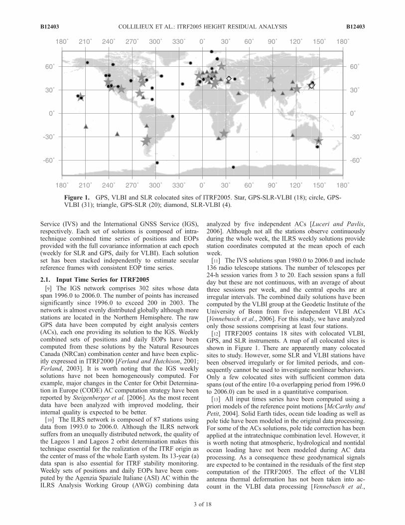
GPS, and SLR instruments. A map of all colocated sites isshown in Figure 1. There are apparently many colocatedsites to study. However, some SLR and VLBI stations havebeen observed irregularly or for limited periods, and con-sequently cannot be used to investigate nonlinear behaviors.Only a few colocated sites with sufficient common dataspans (out of the entire 10-a overlapping period from 1996.0to 2006.0) can be used in a quantitative comparison.[13] All input times series have been computed using a

priori models of the reference point motions [McCarthy andPetit, 2004]. Solid Earth tides, ocean tide loading as well aspole tide have been modeled in the original data processing.For some of the ACs solutions, pole tide correction has beenapplied at the intratechnique combination level. However, itis worth noting that atmospheric, hydrological and nontidalocean loading have not been modeled during AC dataprocessing. As a consequence these geodynamical signalsare expected to be contained in the residuals of the first stepcomputation of the ITRF2005. The effect of the VLBIantenna thermal deformation has not been taken into ac-count in the VLBI data processing [Vennebusch et al.,

Figure 1. GPS, VLBI and SLR colocated sites of ITRF2005. Star, GPS-SLR-VLBI (18); circle, GPS-VLBI (31); triangle, GPS-SLR (20); diamond, SLR-VLBI (4).

B12403 COLLILIEUX ET AL.: ITRF2005 HEIGHT RESIDUAL ANALYSIS

3 of 18

B12403

2006]. The use of current thermal deformation model[McCarthy and Petit, 2004] has been investigated by[Tesmer et al., 2006]. They have shown that this effectmainly causes annual signal up to 0.7 mm and lead toepisodic signal up to ±3 mm in the height component.

2.2. Detrended Height Time Series Computation

[14] IGS, IVS, and ILRS coordinate frame time serieshave been rigorously stacked using the Combination andAnalysis of Terrestrial Reference Frames (CATREF) soft-ware [Altamimi et al., 2002] to estimate positions at areference epoch and velocities for every station. The com-putation strategy is summarized in this section. For moredetails about this approach, see Altamimi et al. [2006,2007].[15] The per technique time series of station positions and

EOPs have been combined, rigorously stacked, using thefollowing relation involving the seven Helmert similarityparameters in a Cartesian frame:

8i; X ik tik� �

¼ X ic þ tik � t0

� �_X ic þ Tk þ DkX

ic þ RkX

ic ð1Þ

where for each point i of the solution k, Xki (tik) is the position

(at epoch tki ) and Xc

i and _X ci are the position (at the reference

epoch t0) and velocity of the stacked solution c. Dk, Tk andRk are the scale factor, the translation vector and the rotationmatrix, respectively, needed to transform the coordinates ofthe combined frame at the mean epoch of the solution k intothe frame of the individual input set k. Tk contains the threeorigin components and Rk the three rotations around thethree axes X, Y, Z, respectively. Thus seven parameters perinput weekly (or session-wise) solution as well as secularcoordinates for every station are estimated using the fullcovariance of every solution to weight the estimation.Frame minimum constraints are added to define the stackedframe and to allow the normal equation inversion [Altamimiet al., 2007].[16] This approach is used to separate global motion and

biases affecting the whole set of stations from the motion ofindividual stations. Here the motion of each station ismodeled as a piecewise linear function so that most of thestation nonlinear motion is left in the postfit residuals. Abreak-wise approach is used to account for discontinuities inthe time series due to any physical motion of the ground,such as earthquakes, or equipment changes. Discontinuityfiles can be found at http://itrf.ensg.ign.fr/. A new stackedstation position is estimated after every offset detected. Inthat case, velocities are usually constrained to be equalbefore and after a discontinuity, except site where earth-quake occurred. A similar velocity constraint is also appliedfor colocated stations. Noncontinuous preseismic and post-seismic deformations have not been modeled in this analysisnor any seasonal term or nonlinear deformation field.[17] The time series residuals of this computation are

assessed in the following. Contrary to the ITRF2005 com-putation, we reject all VLBI sessions having less than fourstations, restricting the number of VLBI sessions to 3259 inthe above computation.

2.3. Network Effect

[18] Geodetic position time series contain nonlinear var-iations which reach several millimeters of amplitude. These

are mainly attributed to loading effects which are notmodeled at the ACs level (see section 2.1) and to remainingsystematic errors. Although equation (1) is weighted by thefull covariance matrix of the positions neither time-corre-lated noise nor nonlinear station motion are modeled. TheHelmert parameters of equation (1) are used to compare thepiecewise linear positions of the stacked frame to thepositions of a frame which undergoes more complex shapedeformation. However, theoretically, this relationship canonly be rigorously applied when the two frames to becompared have a similar shape. A portion of the stationindividual motion may consequently leak into the Helmertparameters. As this effect is dependent on the networkconfiguration, we call it ‘‘network effect’’ in the following,as is commonly done. However, it should be noticed that theamplitude of this effect depends additionally on each stationindividual motion and systematic errors, and on techniqueinternal noise.[19] The analysis of the network effect needs an a priori

knowledge either of the station individual motion or of thetransformation parameters. Blewitt and Lavallee [2000]have analyzed this effect assuming that loading effectsdominate station motions. Tregoning and van Dam [2005]have observed that the scale parameter absorbs stationmotion when transforming station displacements causedby atmospheric loading from a frame centered at the Earth’scenter of mass (CM) to a frame centered at the Earth’ssurface barycenter (CF) using a seven-parameter similarity,but their simulation did not model any other systematicerrors. Lavallee et al. [2006] have also analyzed this effectusing synthetic and real data, mentioning that an annualsignal in the GPS scale is reduced when the crust deforma-tion field is modeled using loading theory. In the context ofITRF computation, and particularly ITRF2005, the scale hasbeen chosen to be estimated to better monitor any distortionof the weekly (or session-wise) frames. Intrinsic IVSsolution scale and ILRS solution translation and scale timeseries are available from Altamimi et al. [2007] (Figures 2and 3). Their rigorous analysis in the scope of networkeffect evaluation requires external information such as aloading model, which is beyond the scope of this paper. Theanalysis of the IGS solution Helmert parameters time seriesthemselves would be useless since IGS weekly frames havealready been expressed in ITRF2000: no seasonal pattern isconsequently detectable in the IGS solution intrinsic scaletime series.[20] We attempt here to evaluate the network effect using

only ITRF2005 data. Our method is to compare stationresidual time series from different IGS subnetworks stackedto give an order of magnitude of the error introduced by thisnetwork effect. The advantage of such an approach is thatno assumption about the signal needs to be made neither forthe residuals nor for the Helmert parameters. Our experi-ment, however, only uses an extract of each covariancematrix. The disadvantage is that the covariances involvingpoints which have been removed are neglected. To circum-vent this omission and to strictly test the geometrical effect,we have only considered station block diagonal covarianceterms in the following either for the subnetwork stacking orfor the full IGS network stacking. We first qualify the IGSnetwork and then evaluate the network effects associatedwith the SLR and VLBI networks.

B12403 COLLILIEUX ET AL.: ITRF2005 HEIGHT RESIDUAL ANALYSIS

4 of 18

B12403

[21] The IGS network has a good global coverage butthere is a concentration of stations in the Northern Hemi-sphere and a varying spatial density. As loading effects and/or systematic errors are regionally correlated (due, forexample, to similar equipment and monumentation in caseof GPS), the aliasing effect is expected to be accentuated.Therefore we have selected a GPS subnetwork which isalmost optimal in terms of spatial density. The Earth’ssurface has been subdivided into 80 faces with almost equalarea, based on the first subdivision of an icosahedroncentered with respect to the Earth [Chambodut et al.,2005]. Only one IGS station has been chosen per face.The selected network covers 61 faces with, on average, 52%of the stations in the X positive hemisphere, 56% in the Ypositive hemisphere and 55% in the Z positive hemisphere(see Table 1). Some of the stations are located in the samesite but operate at different epochs. We have also made three

exceptions to the above rule by using stations located closeto the boundary of an empty face (MDO1, CRO1 andUNSA). The estimation of the 14-parameter similarity(seven for the positions and seven for their time derivatives)between the stacked frame of this subnetwork and thestacked frame of the full IGS network provides the shapedifference between the two solutions. The weighted rootmean square scatter (WRMS) of the transformation is 0.4mm for position and 0.2 mm/a for velocities. The residualtime series of the two stackings are almost identical for thehorizontal components with scatter of 0.5 ± 0.1 mm.However, a difference of 1.2 ± 0.2 mm is observed forthe height component mostly because the two scales differby an annual term of 1 mm of magnitude. Thus we haveobserved that the IGS network effect might have an impactof about 1 mm in the heights when changing to a moreuniformly distributed network. This analysis implicitly

Figure 2. Histograms of the detected frequencies in the ITRF2005 height residuals of the GPStechnique with SNR higher than 3.5. (a) With more than 150 points. (b) Detailed histogram with constantbin width. Orange indicates European stations only (48 time series), and black indicates whole set ofstations (205 time series) (c) Histogram of the detected frequencies in the ITRF2005 height residuals ofthe VLBI technique with SNR higher than 3.5. Twenty residual height time series with more than 150estimated positions are considered. (d) Histogram of the detected frequencies in the ITRF2005 heightresiduals of the SLR technique with SNR higher than 3.5. 28 residual height time series with more than150 estimated positions are considered.

B12403 COLLILIEUX ET AL.: ITRF2005 HEIGHT RESIDUAL ANALYSIS

5 of 18

B12403

assumes that a well distributed network does not suffer fromnetwork effect, which should not be exactly true becausethere is no reason that station individual motions canceleach other exactly. With regards to the relatively small valueobtained and this consideration we keep IGS networkstacking residuals as a reference in the following.[22] To study VLBI and SLR network effects, IGS

colocated subnetworks have been separately extracted fromthe IGS frames building two subsets of data. These subnet-work frames are then stacked with the same strategy as the

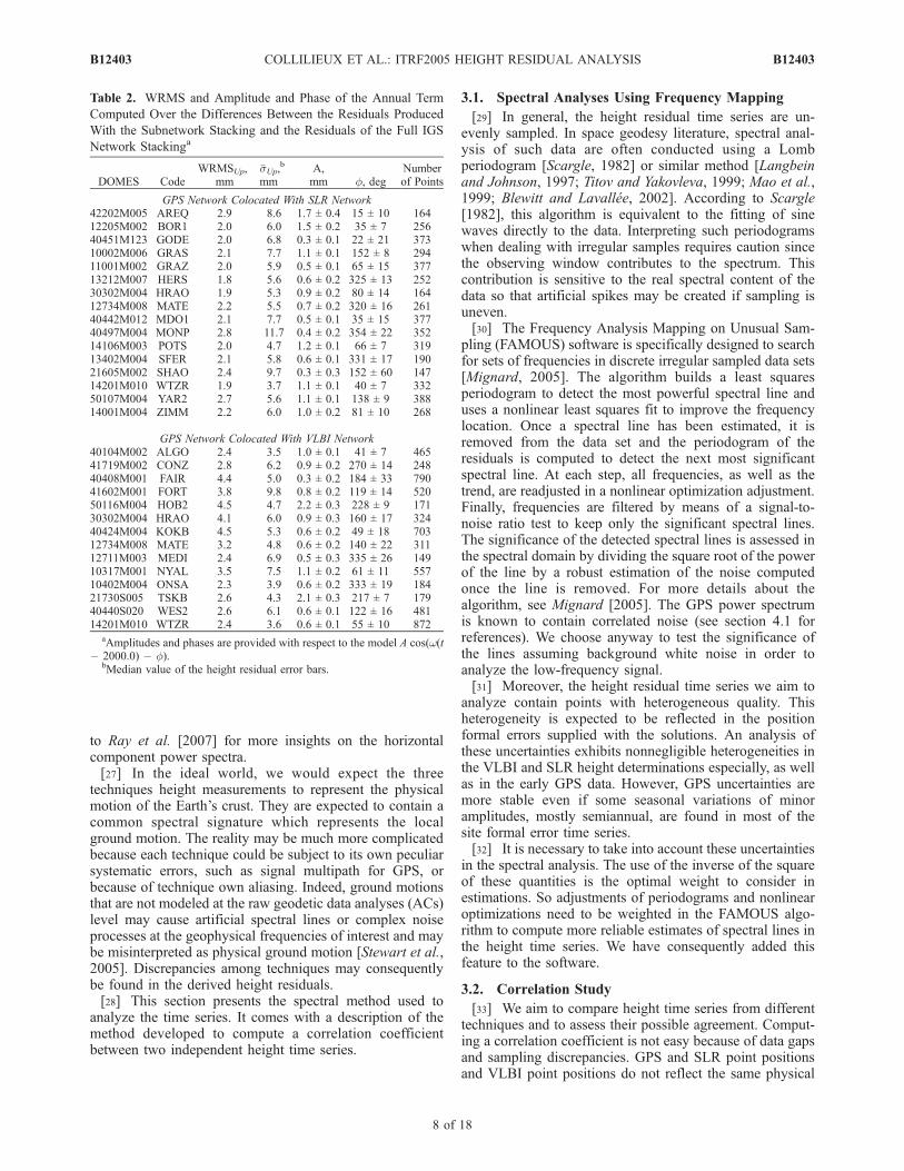
VLBI and SLR input solutions for ITRF2005, using internalconstrains to define the combined frames [Altamimi et al.,2007]. On average, 72% of the SLR stations simultaneouslyoperate with a GPS station. As SLR core stations play animportant role in the SLR analysis, we paid attention toreject all the weeks where more than two IGS stationscolocated with SLR core stations are missing; we assure onaverage that more than 85% of the SLR core stations arerepresented in the colocated GPS subset of data. Thegeometry of the true SLR network is not exactly reproducedin that experiment although the general distribution is quiterepresentative. The stacked solution of this subnetwork iscomparable to the full IGS stacked solution. Indeed, a 14-parameter similarity has been estimated between them overstations having more than 150 points. The WRMS agree-ment of the transformation is at the level of 0.3 mm forpositions and 0.1 mm/a for velocities. It is worth noting thatthere is no significant drift in the translations. The Helmertparameter time series differ from those of the full IGSstacking by 1 mm scatter in each origin component and 2mm in scale. The two sets of residuals are consequentlydifferent. Table 2 shows the computed average scatterbetween the full GPS residuals and colocated GPS networkresiduals in the height component. Horizontal componentsare omitted for clarity but their agreement is at the level of0.8 ± 0.5 mm, whereas it is 2.1 ± 0.3 mm for the heights interm of scatter.[23] The same analysis has been conducted for colocated

VLBI stations where daily solutions of more than fourstations have been used. About 86% of the VLBI stationsoperate simultaneously with IGS stations. The mediannumber of IVS stations is six per session. As VLBI observesat a daily interval, the GPS subnetwork data of the week hasbeen extracted every time a VLBI session has occurred.Similarly, a 14-parameter similarity has been estimatedbetween the stacked frame of this subnetwork and the fullIGS network stacked frame over stations having more than150 points. The WRMS agreement of the transformation is1.3 mm for positions and 0.7 mm/a for velocities. HeightWRMS values are given in Table 2 for stations having morethan 150 points. The horizontal agreement is 1.3 ± 0.5 mmand is 3.0 ± 0.8 mm for the vertical (see Table 2). The levelof scatter due to the network effect, as evaluated here, is stilllower than the uncertainty of the station positions for SLRand VLBI colocated networks.[24] As section 4.1 reveals that the annual harmonic is the

main common spectral line in the IGS, IVS, and ILRSresiduals, we have fitted an annual signal of the residualdifferences with respect to the full IGS reference residualsfor both experiments (see Table 2). The annual signalamplitude is about 1 mm on average for both techniques.There is no significant scale annual signal in the simulatedVLBI scale difference with respect to the full IGS scale. Wenote 0.7 ± 0.1 mm of annual signal in the SLR simulatedscale difference. The difference increases at this frequencycompared to the well-distributed IGS subnetwork to reach0.9 ± 0.1 mm and 1.4 ± 0.2 mm for VLBI and SLR,respectively, with consistent phases for the two signals. Itseems consequently that the scale affects the three techni-ques quite similarly at the annual frequency, mainly due theasymmetry between the Northern and Southern Hemi-

Figure 3. (a) The 4.14 cpy wave estimated in GPS heightresidual time series having SNRs greater than 3.5. (b) The1.00 cpy wave estimated in GPS height residual time serieshaving SNRs greater than 3.5. The norm of arrows providesthe signal amplitude A and the arrow orientation (countedclockwise from the north) indicates the phase f with respectto the model A cos(w(t � 2000.0) � f). The ellipsesrepresent the 95% confidence ellipses.

B12403 COLLILIEUX ET AL.: ITRF2005 HEIGHT RESIDUAL ANALYSIS

6 of 18

B12403

sphere. The effect of these added annual terms may be areduction or an amplification of the real measured annualdisplacement. The phase may shift, but this shift may bereasonably small if the station displacement is much largerthan the added annual error.[25] This experiment provides an indication of the geo-

metrical effect caused by the stacking strategy but does notconstitute an exact answer. Indeed, the SLR and VLBItechniques are not subject to the same systematic errors asGPS is and do not provide the same level of measurementnoise. Thus, although our experiment quite faithfully repro-duces the geometry of the networks, it does not reproducethe exact station position measurement as viewed by theSLR or VLBI techniques. It is, however, reasonable to takethe values of 2 mm and 3 mm as measurement of thenetwork effect for SLR and VLBI, respectively.

3. Height Residual Analysis

[26] Before entering into more details, it is worth brieflydiscussing the scatter of the position residual time series.IGS position residual WRMS is typically at the level of 1.8mm for both horizontal components and 5.3 mm for heights.IVS position residuals have scatter of 3.5 mm and 4.4 mm,

respectively, and ILRS residuals have nearly equal scatter inall components with 8.7 mm horizontally and 8.5 mmvertically for the core stations. Ray et al. [2007] have alsoanalyzed the spectral content of the ITRF2005 ILRS, IVS,and IGS position residuals by stacking the normalizedperiodograms. They conclude that GPS residuals on thethree components are dominated by flicker noise and thatIVS and ILRS power spectra are much whiter. This workuses the same data set, except that we restrict here thenumber of VLBI sessions used. However, this work isdevoted to individual station residual analysis. The verticalcomponent is more interesting to study since loading signalsare larger than for the other components [Farrell, 1972].Systematic errors are expected to be more important too inthat component due mainly to the geometry of the measure-ments, troposphere refraction and data analysis. The scat-tering of SLR residuals on the horizontal component alsodecreases the interest of intercomparing horizontal residualssince only GPS and VLBI techniques would be worthcomparing, restricting the analysis to two independent datasets only. We consequently limit this analysis to the verticalcomponent but the horizontal component issue is addressedif it clarifies or enriches the discussion. The reader may refer

Table 1. IGS Station Subnetwork Selected to Constitute a Spatially Well-Distributed Network

Code NaLong,deg

Lat,deg

WRMS

tstart � tendb Code N

Long,deg

Lat,deg

WRMS

tstart � tendbE, mm N, mm U, mm E, mm N, mm U, mm

ALIC 382 133.9 �23.5 1.6 1.3 5.4 1998.5–2006.0 LHAS 417 91.1 29.5 2.2 2.5 7.2 1996.8–2006.0AOML 308 �80.2 25.6 2.1 1.6 5.6 1998.2–2004.3 MALI 492 40.2 �3.0 3.3 2.2 7.2 1996.1–2006.0ASC1 404 �14.4 �7.9 2.7 1.7 5.8 1996.3–2005.6 MAS1 493 �15.6 27.6 1.7 1.9 5.2 1996.1–2006.0ASPA 151 �170.7 �14.2 3.0 1.6 6.8 2003.1–2006.0 MCM4 501 166.7 �77.8 2.4 1.7 8.4 1996.1–2006.0AUCK 506 174.8 �36.4 3.4 1.6 4.6 1996.1–2006.0 MDO1 515 �104.0 30.5 1.8 1.7 4.6 1996.1–2006.0BAHR 472 50.6 26.1 2.0 2.1 6.0 1996.6–2006.0 MSKU 93 13.6 �1.6 2.5 1.7 4.9 2001.4–2005.3BAKO 319 106.9 �6.5 2.0 2.1 7.3 1998.3–2006.0 NKLG 288 9.7 0.4 1.8 1.5 5.5 2000.3–2006.0BILI 268 166.4 67.9 1.3 2.0 5.3 1999.7–2006.0 NLIB 516 �91.6 41.6 1.8 1.8 5.3 1996.1–2006.0BRAZ 277 �47.9 �15.9 2.0 1.5 8.3 1996.7–2006.0 NOUM 392 166.4 �22.1 3.6 1.8 6.5 1998.2–2006.0BRUS 513 4.4 50.6 1.7 1.6 3.4 1996.1–2006.0 NTUS 347 103.7 1.3 2.0 2.2 5.6 1997.7–2006.0CHAT 507 �176.6 �43.8 2.8 1.8 4.7 1996.1–2006.0 NYAL 487 11.9 78.9 1.5 1.8 5.6 1996.1–2006.0COCO 470 96.8 �12.1 1.9 1.9 4.6 1996.5–2006.0 OHI3 115 �57.9 �63.2 2.0 2.5 6.3 2003.5–2005.9CRO1 479 �64.6 17.7 2.7 1.9 7.0 1996.1–2006.0 OHIG 199 �57.9 �63.2 2.8 3.1 8.7 1996.1–2002.1DAV1 474 78.0 �68.5 1.8 1.7 4.4 1996.1–2006.0 ONSA 509 11.9 57.2 1.3 1.1 3.2 1996.1–2006.0DGAR 370 72.4 �7.2 2.4 2.2 5.1 1996.4–2006.0 PETP 373 158.6 52.9 1.9 1.8 5.6 1998.8–2006.0DRAO 518 �119.6 49.1 1.9 1.8 4.8 1996.1–2006.0 POL2 450 74.7 42.5 1.7 1.6 4.7 1996.1–2006.0EISL 354 �109.4 �27.0 4.2 2.0 7.4 1996.1–2003.8 QAQ1 178 �46.1 60.6 0.9 1.2 5.1 2002.5–2006.0FORT 500 �38.4 �3.9 3.1 2.3 6.6 1996.1–2006.0 RAMO 348 34.8 30.4 3.1 1.9 5.6 1998.5–2006.0GALA 205 �90.3 �0.7 2.1 1.6 4.7 1996.7–2002.9 REYK 507 �22.0 64.0 2.3 1.6 6.3 1996.1–2006.0GLPS 130 �90.3 �0.7 1.3 1.9 3.7 2003.3–2006.0 RIOG 429 �67.8 �53.6 1.5 2.2 5.2 1997.7–2006.0GOLD 518 �116.9 35.2 2.0 2.5 4.5 1996.1–2006.0 SANT 505 �70.7 �33.0 2.1 2.3 6.1 1996.1–2006.0GOUG 249 �9.9 �40.2 3.1 2.1 13.7 1998.7–2006.0 SEY1 145 55.5 �4.6 2.9 2.3 6.5 1999.2–2005.2GUAM 497 144.9 13.5 2.7 2.2 5.3 1996.1–2006.0 STJO 516 �52.7 47.4 1.7 1.4 4.2 1996.1–2006.0HOB2 475 147.4 �42.6 2.2 1.5 5.5 1996.2–2006.0 SUTH 361 20.8 �32.2 2.7 1.5 4.7 1998.3–2006.0HRAO 414 27.7 �25.7 2.0 1.9 5.3 1996.8–2006.0 THTI 355 �149.6 �17.5 2.9 1.9 5.9 1998.5–2006.0IISC 421 77.6 12.9 2.2 1.5 7.1 1997.4–2006.0 TIXI 369 128.9 71.5 1.7 2.3 6.4 1998.8–2006.0INVK 211 �133.5 68.1 1.7 2.3 8.9 2001.9–2006.0 TOW2 384 147.1 �19.2 2.0 1.6 4.6 1998.5–2006.0IRKT 495 104.3 52.0 2.0 2.2 8.1 1996.1–2006.0 TSKB 504 140.1 35.9 2.3 2.4 6.8 1996.1–2006.0ISPA 84 �109.3 �27.0 1.8 1.2 5.9 2004.2–2006.0 UNSA 271 �65.4 �24.6 1.8 1.6 6.0 2000.3–2006.0KERG 488 70.3 �49.2 2.0 2.2 4.3 1996.1–2006.0 VESL 257 �2.8 �71.6 1.7 1.7 7.3 1998.8–2006.0KIT3 392 66.9 39.0 2.1 2.6 5.0 1996.1–2006.0 VILL 500 �4.0 40.3 1.5 1.4 3.7 1996.1–2006.0KOKB 495 �159.7 22.0 2.8 1.8 5.5 1996.1–2006.0 WUHN 484 114.4 30.4 2.3 1.9 6.5 1996.6–2006.0KOUR 482 �52.8 5.2 2.4 2.6 6.7 1996.1–2006.0 YAR2 501 115.4 �28.9 2.3 1.9 6.3 1996.1–2006.0KWJ1 277 167.7 8.7 3.1 2.3 6.9 1996.2–2002.6

aNumber of weekly estimated positions available over the interval 1996.0–2006.0.bData span of the station.

B12403 COLLILIEUX ET AL.: ITRF2005 HEIGHT RESIDUAL ANALYSIS

7 of 18

B12403

to Ray et al. [2007] for more insights on the horizontalcomponent power spectra.[27] In the ideal world, we would expect the three

techniques height measurements to represent the physicalmotion of the Earth’s crust. They are expected to contain acommon spectral signature which represents the localground motion. The reality may be much more complicatedbecause each technique could be subject to its own peculiarsystematic errors, such as signal multipath for GPS, orbecause of technique own aliasing. Indeed, ground motionsthat are not modeled at the raw geodetic data analyses (ACs)level may cause artificial spectral lines or complex noiseprocesses at the geophysical frequencies of interest and maybe misinterpreted as physical ground motion [Stewart et al.,2005]. Discrepancies among techniques may consequentlybe found in the derived height residuals.[28] This section presents the spectral method used to

analyze the time series. It comes with a description of themethod developed to compute a correlation coefficientbetween two independent height time series.

3.1. Spectral Analyses Using Frequency Mapping

[29] In general, the height residual time series are un-evenly sampled. In space geodesy literature, spectral anal-ysis of such data are often conducted using a Lombperiodogram [Scargle, 1982] or similar method [Langbeinand Johnson, 1997; Titov and Yakovleva, 1999; Mao et al.,1999; Blewitt and Lavallee, 2002]. According to Scargle[1982], this algorithm is equivalent to the fitting of sinewaves directly to the data. Interpreting such periodogramswhen dealing with irregular samples requires caution sincethe observing window contributes to the spectrum. Thiscontribution is sensitive to the real spectral content of thedata so that artificial spikes may be created if sampling isuneven.[30] The Frequency Analysis Mapping on Unusual Sam-

pling (FAMOUS) software is specifically designed to searchfor sets of frequencies in discrete irregular sampled data sets[Mignard, 2005]. The algorithm builds a least squaresperiodogram to detect the most powerful spectral line anduses a nonlinear least squares fit to improve the frequencylocation. Once a spectral line has been estimated, it isremoved from the data set and the periodogram of theresiduals is computed to detect the next most significantspectral line. At each step, all frequencies, as well as thetrend, are readjusted in a nonlinear optimization adjustment.Finally, frequencies are filtered by means of a signal-to-noise ratio test to keep only the significant spectral lines.The significance of the detected spectral lines is assessed inthe spectral domain by dividing the square root of the powerof the line by a robust estimation of the noise computedonce the line is removed. For more details about thealgorithm, see Mignard [2005]. The GPS power spectrumis known to contain correlated noise (see section 4.1 forreferences). We choose anyway to test the significance ofthe lines assuming background white noise in order toanalyze the low-frequency signal.[31] Moreover, the height residual time series we aim to

analyze contain points with heterogeneous quality. Thisheterogeneity is expected to be reflected in the positionformal errors supplied with the solutions. An analysis ofthese uncertainties exhibits nonnegligible heterogeneities inthe VLBI and SLR height determinations especially, as wellas in the early GPS data. However, GPS uncertainties aremore stable even if some seasonal variations of minoramplitudes, mostly semiannual, are found in most of thesite formal error time series.[32] It is necessary to take into account these uncertainties

in the spectral analysis. The use of the inverse of the squareof these quantities is the optimal weight to consider inestimations. So adjustments of periodograms and nonlinearoptimizations need to be weighted in the FAMOUS algo-rithm to compute more reliable estimates of spectral lines inthe height time series. We have consequently added thisfeature to the software.

3.2. Correlation Study

[33] We aim to compare height time series from differenttechniques and to assess their possible agreement. Comput-ing a correlation coefficient is not easy because of data gapsand sampling discrepancies. GPS and SLR point positionsand VLBI point positions do not reflect the same physical

Table 2. WRMS and Amplitude and Phase of the Annual Term

Computed Over the Differences Between the Residuals Produced

With the Subnetwork Stacking and the Residuals of the Full IGS

Network Stackinga

DOMES CodeWRMSUp,

mm�sUp,

b

mmA,mm f, deg

Numberof Points

GPS Network Colocated With SLR Network42202M005 AREQ 2.9 8.6 1.7 ± 0.4 15 ± 10 16412205M002 BOR1 2.0 6.0 1.5 ± 0.2 35 ± 7 25640451M123 GODE 2.0 6.8 0.3 ± 0.1 22 ± 21 37310002M006 GRAS 2.1 7.7 1.1 ± 0.1 152 ± 8 29411001M002 GRAZ 2.0 5.9 0.5 ± 0.1 65 ± 15 37713212M007 HERS 1.8 5.6 0.6 ± 0.2 325 ± 13 25230302M004 HRAO 1.9 5.3 0.9 ± 0.2 80 ± 14 16412734M008 MATE 2.2 5.5 0.7 ± 0.2 320 ± 16 26140442M012 MDO1 2.1 7.7 0.5 ± 0.1 35 ± 15 37740497M004 MONP 2.8 11.7 0.4 ± 0.2 354 ± 22 35214106M003 POTS 2.0 4.7 1.2 ± 0.1 66 ± 7 31913402M004 SFER 2.1 5.8 0.6 ± 0.1 331 ± 17 19021605M002 SHAO 2.4 9.7 0.3 ± 0.3 152 ± 60 14714201M010 WTZR 1.9 3.7 1.1 ± 0.1 40 ± 7 33250107M004 YAR2 2.7 5.6 1.1 ± 0.1 138 ± 9 38814001M004 ZIMM 2.2 6.0 1.0 ± 0.2 81 ± 10 268

GPS Network Colocated With VLBI Network40104M002 ALGO 2.4 3.5 1.0 ± 0.1 41 ± 7 46541719M002 CONZ 2.8 6.2 0.9 ± 0.2 270 ± 14 24840408M001 FAIR 4.4 5.0 0.3 ± 0.2 184 ± 33 79041602M001 FORT 3.8 9.8 0.8 ± 0.2 119 ± 14 52050116M004 HOB2 4.5 4.7 2.2 ± 0.3 228 ± 9 17130302M004 HRAO 4.1 6.0 0.9 ± 0.3 160 ± 17 32440424M004 KOKB 4.5 5.3 0.6 ± 0.2 49 ± 18 70312734M008 MATE 3.2 4.8 0.6 ± 0.2 140 ± 22 31112711M003 MEDI 2.4 6.9 0.5 ± 0.3 335 ± 26 14910317M001 NYAL 3.5 7.5 1.1 ± 0.2 61 ± 11 55710402M004 ONSA 2.3 3.9 0.6 ± 0.2 333 ± 19 18421730S005 TSKB 2.6 4.3 2.1 ± 0.3 217 ± 7 17940440S020 WES2 2.6 6.1 0.6 ± 0.1 122 ± 16 48114201M010 WTZR 2.4 3.6 0.6 ± 0.1 55 ± 10 872

aAmplitudes and phases are provided with respect to the model A cos(w(t� 2000.0) � f).

bMedian value of the height residual error bars.

B12403 COLLILIEUX ET AL.: ITRF2005 HEIGHT RESIDUAL ANALYSIS

8 of 18

B12403

quantity: GPS and SLR positions are weekly integrations ofmean motion whereas VLBI positions are daily integrations.Averaging VLBI data at the GPS or SLR sampling wouldnot be reasonable because of VLBI data sparseness. Wehave adopted a time evolution model of the data to deal withdata gaps and this heterogeneous sampling. In doing so, weadd stochastic information to model the time evolution ofthe data. The GPS and SLR averaging process of dailypositions also need to be modeled in the comparisonmethod.3.2.1. Correlation Computation Equations[34] Our method is based on a nonadaptative Kalman

filter: a complete review of Kalman filtering and basicrandom processes is given, for example, by Herring et al.[1990]. The state-space model used in the Kalman filterformalism is particularly adapted to describe the timeevolution of a random process. The random process, calledthe state, does not necessarily need to be directly observ-able: the observations, here a pair of height residuals fromtwo distinct techniques, can be related to the randomprocess as a linear combination, plus an additive noise.We present the model used to compare weekly time series todaily time series, for example, GPS or SLR residual heighttime series and VLBI residual height time series. In ourcase, we would like to estimate the daily height motionviewed by the two techniques. In the following, we call thisdaily height the state height. Thus our state vector containsat least two parameters, one for the state height as viewedby each technique. However, GPS and SLR height residualsrepresent a weekly mean height with an average of sevenconsecutive daily height parameters. Seven state parametersare then needed for GPS or SLR vectors and one stateparameter is needed for each VLBI state height which isdirectly observable.[35] The dynamics of the state parameters are given in the

Kalman filter state equation. Two consecutive positions zt+1and zt are modeled to differ by a white noise contribution,the innovations Vt:

Ztþ1 ¼ AtZt þ Vt

zvlbitþ4ð Þ

zgps

t�2ð Þ

zgps

t�1ð Þ

zgps

tð Þ

zgps

tþ1ð Þ

zgps

tþ2ð Þ

zgps

tþ3ð Þ

zgps

tþ4ð Þ

266666666666666664

377777777777777775

¼

1 0 0 0 0 0 0 0

0 0 1 0 0 0 0 0

0 0 0 1 0 0 0 0

0 0 0 0 1 0 0 0

0 0 0 0 0 1 0 0

0 0 0 0 0 0 1 0

0 0 0 0 0 0 0 1

0 0 0 0 0 0 0 1

266666666666664

377777777777775

zvlbitþ3ð Þ

zgps

t�3ð Þ

zgps

t�2ð Þ

zgps

t�1ð Þ

zgps

tð Þ

zgps

tþ1ð Þ

zgps

tþ2ð Þ

zgps

tþ3ð Þ

266666666666666664

377777777777777775

þ

vvlbitþ3ð Þ0

0

0

0

0

0

vgps

tþ3ð Þ

2666666666666664

3777777777777775

ð2Þ

where z(t)vlbi, z(t)

gps are the state daily heights viewed by VLBIand GPS, respectively, at the epoch t. The innovations, v(t)

vlbi

and v(t)gps, may be different for each technique but are

assumed to be correlated. This correlation is modeled in the

innovation vector V(t) variance-covariance matrix, assumedto be

Var Vtð Þ ¼

s2wnvlbi 0 . . . . . . 0 rswnvlbiswngps

0 0 0

..

. . .. ..

.

..

. . .. ..

.

0 0 0

rswnvlbiswngps 0 . . . . . . 0 s2wngps

266666664

377777775ð3Þ

The correlation coefficient r and the white noise variancesswnvlbi2 and swngps

2 are unknown and are our parameters ofinterest.[36] Our sampling problem is solved in the measurement

equation of the Kalman filter. When GPS and VLBI data areavailable at 3-d intervals, our observation equation iswritten as

hvlbitþ3ð Þ

hgps

tð Þ

" #¼

1 0 0 0 0 0 0

0 17

17

17

17

17

17

" #

zvlbitþ3ð Þ

zgps

t�3ð Þ

zgps

t�2ð Þ

zgps

t�1ð Þ

zgps

tð Þ

zgps

tþ1ð Þ

zgps

tþ2ð Þ

zgps

tþ3ð Þ

266666666666666664

377777777777777775

þuvlbi

tþ3ð Þ

ugps

tð Þ

" #

Ht ¼ CtZt þ Ut ð4Þ

where h(t)vlbi and h(t)

gps are the height residuals at the epoch t. Inequation (4), we assume that the VLBI measurement is anobservation of the daily position which is a firstapproximation because the middle of the session does notcoincide with the middle of the day. The random process Ut

models the measurement noise which is assumed to beuncorrelated. The covariance matrix of the measurementnoise is

Var Utð Þ ¼s0vlbi

2s2vlbiobs tþ3ð Þ 0

0 s0gps2s2

gpsobs tð Þ

" #ð5Þ

[37] An indication of the measurement noise is providedwith the height residuals through the covariance matrix ofthe associated observations where sgpsobs

2 and svlbiobs2 are

taken from. Our combination experiment encourages us torescale these quantities, which are overly optimistic. This isdone through the variance factor parameters s0gps

2 and s0vlbi2 .

When one of the two observations is not available, thecorresponding line of this equation is removed.[38] Equations (2) and (4) are used to estimate the state

vector and its covariance matrix at daily sampling from thefirst day to the last day of common observation span, byusing the Kalman filter equations [Herring et al., 1990].However, the matrices of this model are dependent on some

B12403 COLLILIEUX ET AL.: ITRF2005 HEIGHT RESIDUAL ANALYSIS

9 of 18

B12403

parameters which are the following: the innovations var-iances swngps

2 and swnvlbi2 and their correlation r and scaling

factors s0vlbi2 and s0gps

2 . These five parameters are estimatedby maximum likelihood (ML).[39] The log likelihood of the observation vector Ht is

built according to Gourieroux and Monfort [1997] underGaussian assumption by

log LHð Þ Ht; qð Þ ¼ � 1

2

Xnt¼1

log det Var Htþ1jt� �

qð Þ� � � �

� 1

2

Xnt¼1

dim Htð Þ log 2pð Þ½

� 1

2

Xnt¼1

Ht � Htþ1jt qð Þ� �T

Var Htþ1jt qð Þ� ��1

Ht � Htþ1jt qð Þ� �

where H t+1jt and var(H t+1jt) are the prediction of theobservation at time t + 1 and its covariance matrix builtusing the whole set of observations before time t,respectively. These quantities are computed using theestimates of the Kalman filter and their covariance matrices[Gourieroux and Monfort, 1997]. According to equation(6), the Kalman filter needs to be run fully forward toevaluate the log likelihood. This log likelihood is minimizedusing the downhill simplex method [Press et al., 1996].[40] The Kalman filter model is slightly modified to

estimate the correlation coefficient between SLR and GPSdata. We assume the SLR positions to be mean motions overan entire week although this is not strictly true. Indeed, theSLR network only tracks satellites when they are observableand when weather conditions allow. The same can also besaid for GPS where observations for an entire week are notalways used for every station. However, the information ofthe midpoint epoch of the observations is stored in the IGSsolution files. We consider this epoch to be the epoch of aweekly position because the information of the exactintegration time is not always directly available. With

respect to these concerns, the sample epochs are not equal.The previous model has to be modified to use 14 statemodel parameters to represent the averaging process in theobservation equation. Observations at the same epoch canbe used when they are both available, equation (4) becomes

hslrtð Þ

hgps

tð Þ

" #¼

17I7 0

0 17I7

� �zslrt�3ð Þ

..

.

zslrtþ3ð Þ

zgps

t�3ð Þ

..

.

zgps

tþ3ð Þ

266666666664

377777777775þ

uslrtð Þ

ugps

tð Þ

" #ð7Þ

where I7 is the identity matrix.3.2.2. Estimator of the Parameter Variances[41] In the case of an asymptotic normal distribution for

the ML estimator, the covariance matrix of the parameterscan be estimated analytically. It is the opposite of theinverse of the Hessian matrix of the log likelihood functioncomputed at the point of the maximum. For example, thisestimator has been used by Zhang et al. [1997] to estimatethe variance of their ML estimator of the random walk andwhite noise variances which were assumed to model thenoise in GPS position time series. Conversely, Langbeinand Johnson [1997] have proposed a method which relieson a Monte Carlo simulation to compute error bars. In thefollowing, we check if the Hessian matrix can be used tocompute the estimate covariance matrix in our specificapplication.[42] To do so, simulated data must first be generated and

used as input to our estimator to compute a scatter of theestimated parameters around the simulated values. Empiri-cal mean square errors (MSE) are compared to the secondderivative mean values in Tables 3 and 4 for 1000 simu-lations of 350 points without gaps. The variance estimatesprovide similar results. When comparing VLBI and GPS theinnovation variance of VLBI is better determined than inGPS because the VLBI daily motion is directly observed.Conversely, the variance factor of GPS measurement noiseis better determined. Indeed, it is easier to distinguish themeasurement noise from the state dynamics, which areaveraged in the case of the GPS model.[43] As the MSE computation is time consuming, the

second derivative evaluation to compute uncertainties forestimated parameters is retained.

4. Results

4.1. Spectral Content

[44] All stations having more than 150 estimated posi-tions are analyzed to search for up to 10 significantfrequencies, each with signal-to-noise ratio (SNR) higher

Table 3. Results of the Tests of the ML Estimator on Synthetic

GPS and VLBI Time Seriesa

sVLBI,mm d1/2

sGPS,mm d1/2 r sVLBI

0 sGPS0

Simulatedparameters

0.600 0.600 0.300 1.000 1.000

Mean of estimatedparameters

0.596 0.597 0.306 0.999 0.999

Square root ofmean variances

0.064 0.072 0.148 0.055 0.042

Square rootof the MSE

0.067 0.074 0.146 0.055 0.042

aThere are 350 points per technique; 1000 simulations. The parametersused to generate these simulated data are listed as well as the averageestimates and the mean square error (MSE).

Table 4. Results of the Tests of the ML Estimator on Synthetic GPS and SLR Time Seriesa

sSLR, mm d1/2 sGPS, mm d1/2 r sSLR0 sGPS

0

Simulated parameters 0.600 0.600 0.300 1.000 1.000Mean of estimated parameters 0.597 0.595 0.289 0.999 1.001Square root of mean variances 0.073 0.073 0.156 0.042 0.042Square root of the MSE 0.072 0.073 0.157 0.042 0.043

aThere are 350 points per technique; 1000 simulations.

ð6Þ

B12403 COLLILIEUX ET AL.: ITRF2005 HEIGHT RESIDUAL ANALYSIS

10 of 18

B12403

than 3.5. As the frequencies are estimated in a nonlinearleast squares adjustment, the uncertainties on the frequencylocations can be computed as well as the uncertainties forthe amplitudes and phases. The precision of the frequencylocation is mainly related to the presence of noise in the dataand to the number of data samples. Assuming normalbackground decorrelated noise and given our data span,we estimate the precision of the annual frequency locationto be on the order of 10�2 cpy for SLR data and better than10�2 cpy for VLBI and GPS. The width of the detectedspectral lines in the frequency domain cannot be thinnerthan 0.106, 0.092, and 0.052 cpy for GPS, SLR, and VLBI,respectively, which give an order of magnitude of themaximum spectral resolution.[45] The assessment of the detected frequencies is pre-

sented as histograms of the proportion of stations for whichdetected frequencies in a given frequency bin exist. Thespectral bins are chosen to be constant in the logarithmicscale such that the logarithm of the ratio of two consecutivebin frequencies is equal to 0.1 (see Figures 2a, 2c, and 2d).It should be noted that only stations providing data lengthslonger than 2 times the period of the spectral line arecounted in the bins of these histograms.[46] The GPS power spectrum has already been exten-

sively analyzed during the last decade. It contains a flickernoise background spectrum and white noise [Zhang et al.,1997; Mao et al., 1999; Williams et al., 2004; Le Bail et al.,2007]. Annual and semiannual frequencies have also beenwidely detected [Mao et al., 1999; Blewitt and Lavallee,2000; Dong et al., 2002]. Blewitt and Lavallee [2002] havealso reported other annual frequency harmonics. UsingITRF2005 IGS residuals, Ray et al. [2007] have investigat-ed these harmonics accurately. They have shown that thesefrequencies were not exactly located at integer values eitheron vertical or horizontal components. A model of harmonicsof the 1.04 cpy frequency fits their locations very well. Theauthors have suggested that these could be systematic errorsrelated to the GPS satellite orbits combined with thegeometry of the measurements. Figure 2a shows the resultsof our study. The proportion of significant spectral lines inevery frequency band with SNR higher than 3.5 is pre-sented. This analysis reveals that 71% of GPS station heightresidual time series have a significant signal at a frequencylocated between 0.95–1.05 cpy with SNR higher than 3.5.This annual frequency comes with a semiannual frequency,and frequencies at the previously mentioned harmonics.This study gives median frequencies of 3.09 cpy and4.14 cycles per year with scatters of 0.09 cpy for thesetwo frequencies (see Figure 2b). These are consistent withthe values 3.12 and 4.16 cpy suggested by Ray et al. [2007].It confirms that these harmonics are detectable in theindividual time series. The annual and semiannual as wellas 3.09 and 4.14 cpy signals have been estimated for everyheight time series with a significant spectral line detectedaround 4.14 cpy. Figure 3a shows the distribution of the4.14 cpy spectral line using the convention of Dong et al.[2002] for the representation: the norms of the vectorsindicate the signal amplitudes whereas their orientationsgive the phases. For most stations, the amplitude of thesignal is less than 2 mm for these two frequencies. Thestations having the most powerful signals at 4.14 cpy arelocated at high latitude and notably in North America. The

amplitude reaches 4.6 ± 0.5 mm at the GPS Alert station innortheastern Canada with SNR up to 10. Moreover, it isnoteworthy that some areas of the world like North Amer-ica, western Europe and the Persian Gulf exhibit a clearspatial correlation of this signal. These harmonics are alsodetectable in the horizontal position time series with lessthan half a millimeter of amplitude on average.[47] The VLBI histogram in Figure 2c has been built with

20 stations. The ITRF2005 VLBI residual height time seriescontain mainly white noise [Ray et al., 2007], but withhigher level than GPS. As a consequence, the SNR is muchlower than for GPS. Only the annual frequency seems to belargely detected in the analyzed set. We can also notice afew low frequencies, but it represents one or two stations ineach lower bin. Half of the analyzed time series havesignificant power (SNR >3.5) between 0.95–1.05 cpy.Some few frequencies have been detected at higher location,but we interpret them as noise. No other frequency than theannual has been largely detected in the horizontal compo-nent as well. We notice that the semiannual signaturereported by Titov and Yakovleva [1999] and Petrov andMa [2003] has not been detected here. Tesmer et al. [2007]have, however, reported a semiannual signal in the VLBIscale as well as annual. This signal has been shown to berobust whatever the mapping function used to model thetropospheric delay. We detect annual and semiannual sig-nals as well in the IVS solution scale at the level of 2.9 ±0.1 mm and 1.2 ± 0.1 mm, respectively, for these twofrequencies. We have computed these values using dataafter 1993.0 because the number of stations has increasedsince that time [Tesmer et al., 2007]. Moreover, we thinkthat the network effect could add noise processes whichgenerally decrease the signal-to-noise ratio of the underly-ing signals.[48] The SLR power spectrum is more evenly dispersed.

Figure 2d has been obtained by analyzing 28 position timeseries. There are several frequency intervals containingsignificant spectral lines. The annual frequency is detectedin 8 time series in the interval 0.95–1.05 cpy. Semiannualsignals are detected in Riyadh, Arequipa, and Quincy timeseries. Riyadh station is not collocated, and the last two timeseries are not consistent with the colocated GPS data. Wedetect other groups of frequencies for some stations. Thereis a wide range of frequencies detected between 0.75 and0.9 cpy, as well as some lower frequencies. The horizontalpower spectra contain, however, few significant spectrallines as well, except the annual signature and some isolatedgroups of frequencies representing few stations. There istherefore no global signature at fixed frequencies in theILRS residuals.[49] The GPS power spectrum contains important power

at low frequency. In fact, the power spectrum characteristicsdepend on the area of the world. For example, Figure 2bshows frequencies distribution in the global spectrum overEurope compared to the full network. The 6th anomalousharmonic is detectable in this area for a few stations.European stations also contain more power between 0.33and 0.36 cpy. A fit at 0.35 cpy in the height residuals timeseries having more than 400 estimated positions reveals inphase signal over central Europe up to 2 mm. This resultreveals possible spatially correlated low-frequency signalsin the GPS data. This type of signal is usually analyzed as

B12403 COLLILIEUX ET AL.: ITRF2005 HEIGHT RESIDUAL ANALYSIS

11 of 18

B12403

being part of a flicker noise background spectrum and isanalyzed in term of variance level. Such analysis shows thatthe phase is worth studying. Nevertheless, such results needto be analyzed with caution because IGS data have not beencomputed homogeneously over time. Such low-frequencysignals would be worth studying with reprocessed GPS timeseries such as the ones computed at the Technical Univer-sities of Munich and Dresden [Steigenberger et al., 2006].

4.2. Annual Spectral Line

[50] The annual signal of ITRF2005 height residuals iscarefully studied as it is the only common spectral feature ofthe three observing techniques. An annual signal, as well asa constant, have been fitted by weighted least squares foreach colocated site height residual time series with morethan 150 points and for all GPS stations with a significantannual frequency (SNR >3.5). We consequently assumehere that the annual amplitude of the signal, as well as itsphase are constant with time. A semiannual signal has beenfitted simultaneously for GPS stations. The order of mag-nitude of the GPS annual amplitudes is less than 1 cm, themaximum being found at the Brazilia GPS station (BRAZ).The median value lies around 3–4 mm. Figure 3b shows thedistribution of the estimated annual GPS signals using theconventions of Dong et al. [2002] for the representation.Thus a vector pointing directly north describes an annualmotion having a maximum in January or a vector pointingeast describes an annual motion with its maximum in April.Figure 3b shows all stations having a significant annualsignal detected with the previous method. It exhibits clearregional correlations in Australia, South Africa, westernEurope and North America.[51] Figure 4 displays the annual signals estimated for all

colocated techniques. The significant annual signals for allother GPS stations are also shown. The annual signalsmeasured by the three techniques are in agreement at afew colocated sites. The list of these sites is given in Table 5together with their annual signal estimates. A few sitesexhibit impressive agreement both in amplitude and phase,such as the Yarragadee, Canberra, Hobart and Hartebees-thoek sites. This agreement is reinforced by the spatialconsistency of GPS annual signals fitted at the otherregional sites; see the map of Australia in Figure 4. Whatcan be clearly seen is that the three techniques reflect acommon spatially correlated signal. As the three techniquesare independent regarding their measurement principles,this agreement may be interpreted as evidence of anunderlying geophysical signature. We consequently suggestthis area, as well as the south of Africa and eastern NorthAmerica for geodynamic investigation. The total contribu-tion of the annual loading effects has been studied byMangiarotti et al. [2001]. Plates 1 to 3 of Mangiarotti etal., 2001], which present annual amplitude and phases ofthe total annual loading effect, can be compared to Figure 4.The case of sites in Europe is also instructive. The GPSannual signal in eastern Europe is spatially coherent. MateraVLBI station (Italy) seems to follow the phase of the motionand Potsdam SLR station (Germany) also although theestimated signal is less well determined. However, Wettzell(Germany) and Zimmerwald stations (Switzerland) do notexhibit agreement at that frequency. van Dam et al. [2007]have also compared IGS residual position time series after

having corrected them for the effect of atmosphere andocean loads to their GRACE water loading displacementmodel. The agreement was also very poor notably at thecoastal area.[52] We observe for some residual time series, mainly

GPS, very close spectral lines located near the annualfrequency and its harmonics. Our interpretation of suchspectral line groups is a time-varying behavior by theunderlying periodic source. We have noticed that a sec-ond-order polynomial representation of the amplitude andphase of the annual signal approximates very well thesignal, for example, for the GPS station MONP height timeseries.

4.3. Colocated Sites

4.3.1. Correlations[53] Our method is illustrated using the results for Harte-

beesthoek (South Africa). The estimated correlation be-tween VLBI and GPS height time series is 0.88 ± 0.09with comparable innovation variances, meaning that thesetwo signals are very consistent. The smoothed GPS andVLBI daily height time series can be estimated with the helpof the Kalman filter equations [Gourieroux and Monfort,1997], theorem 15.5. The plot of these signals is shown inFigure 5a. The smoothed signals have comparable ampli-tudes and are very similar due to the important value of thecorrelation coefficient. The VLBI signal is much moresmoothed than the GPS signal because the uncertainties ofthe original height time series are higher and moreoverrescaled by a factor of 1.4. Figure 5a illustrates that thismethod can be used to interpolate a position time series in acolocated site when data are missing. The SLR andGPS signals for this site are also very consistent at thelevel of 0.68 ± 0.15 with comparable levels of variance (seeTable 6).[54] The results of site correlation estimates are computed

for pairs of time series with more than 200 estimatedpositions in the common data period. The results are givenin Table 6 for GPS and VLBI, for GPS and SLR and forVLBI and SLR comparisons, ordered by colocation site. Wehave observed unbalanced solutions when the numbers ofdata points of the two series are small or when the numberof data points are not of the same order. This is the case forthe Hobart comparison, see Table 7. The minimizationalgorithm has converged to null VLBI innovation variancefor Tsukuba correlation estimation between VLBI and GPStime series and between VLBI and SLR data at Matera. Theresults of these comparisons have consequently been omit-ted in Table 6, since in that case, the correlation coefficientis not meaningful.[55] The first general comment concerns the estimation of

the measurement noise variance factors. The ratio betweenthe VLBI and GPS error bar factors lies mostly between 3and 4 whereas it is around 4 to 7 for SLR and GPS timeseries comparisons. The correlation study between VLBIand SLR confirms these values since the ratio between SLRand VLBI error bar factors is around 1.5. According to thesevalues, ILRS and IVS standard deviations are optimistic butthe network effect may add scatter in the height time seriesas seen in section 2.3. Our method seems to underevaluatethe GPS variance factor. This is in fact an expected resultbecause, compared to SLR and VLBI, the GPS background

B12403 COLLILIEUX ET AL.: ITRF2005 HEIGHT RESIDUAL ANALYSIS

12 of 18

B12403

power spectrum is dominated by correlated noise processes.The measurement noise is assumed to be uncorrelated in ourhypothesis; therefore the correlated part of the measurementnoise is consequently absorbed in the GPS state height. The

correlation coefficients between GPS and VLBI lie between0.5 and 0.9 with reasonable error bar values. AlthoughVLBI state variances are always lower than GPS variances,probably because of GPS correlated measurement noise, the

Figure 4. Vertical annual motions estimated for colocated GPS (red), VLBI (green), and SLR (blue)stations. Gray arrows represent the vertical annual motions for noncolocated GPS stations having SNRgreater than 3.5. See Figure 3 for the plot conventions.

B12403 COLLILIEUX ET AL.: ITRF2005 HEIGHT RESIDUAL ANALYSIS

13 of 18

B12403

innovation variances have comparable values with respectto their error bars. These results reflect the good consistencybetween GPS and VLBI heights at every colocated site withsufficient data. Figure 5d also displays IVS and IGS residualheight time series as well as their smoothed values at NyAlesund. We observe some periods of time when these tworesidual time series disagree.[56] The SLR results are more disparate. SLR height

standard deviations need to be rescaled by an average factorof 2. We notice that some sites have heterogeneous levels ofvariances for the GPS and SLR innovation processes.Figure 5c shows, for example, ILRS and IGS heightresidual time series at Wettzell (Europe) where this config-uration is encountered. The consistency is achieved whenthese quantities are of the same order of magnitude withreasonable values of the correlation coefficient like atHartebeesthoek, Potsdam, Arequipa, or Yarragadee (seeFigure 5b).[57] Unfortunately, the comparison of SLR and VLBI

data is only possible for two colocated sites (see Table 6)because of a lack of common data. Contrary to Wettzell,Hartebeesthoek shows close agreement between VLBI andSLR. This colocated site exhibits consistent residual heighttime series for all three techniques whatever the time seriesbeing compared.4.3.2. Interannual and Intra-annual Variations[58] We focus in this part on the interannual variations by

first assessing the extent to which the correlation coeffi-cients in section 4.3.1 can be attributed to the annualsignals. To answer this question, colocated sites withconsistent detected annual signals are studied. A commonannual signal is first fitted at every colocated site usingVLBI, GPS and SLR data where at least a couple of fitted

annual signals are consistent. These data are weighted in theestimation process with the variance factor values estimatedby MLE (see Table 6). As previously mentioned, the GPSvariance factors from Table 6 are lower than those of theother techniques. The GPS signal will consequently domi-nate the estimated annual term. The combined annual valuesare given in Table 7. At each of these sites, the estimatedsignal is removed from the input data and a new correlationcoefficient is estimated with the previous method for coupleof time series having more than 200 points in their commondata period. Results are shown in Table 7.[59] The measurement noise standard deviation factors of

all sites stay unchanged compared to Table 6. The innova-tion variances and correlation coefficients slightly decreasefor most of the sites but do not decrease as much as wemight have expected. The reason is that the time seriesscatter do not decrease so much when an annual wave isremoved. Indeed, a single wave is not sufficient to representthe annual pattern being repeated in the time series, thesebeing subject to significant interannual variations. Thus, formost of these sites, the annual signal spectral line is not theonly one responsible for the consistency observed, notablybetween GPS and VLBI time series. The SLR and GPS timeseries comparison in Yarragadee demonstrates that SLR andGPS in this site have mainly a consistent annual signal andprobably not more. Once removed, the correlation obtained,for equal state variances, is no longer significant.

5. Conclusion

[60] For the first time, combined input TRF time series ofindependent techniques have been analyzed homogeneouslyfor the ITRF2005 computation. It is therefore a greatopportunity to assess the agreement between the VLBI,GPS and SLR time series of positions. The key feature ofsuch comparisons relies on colocated sites where instru-ments of different techniques operate close to each other.[61] The residual height time series from a rigorous

stacking have been compared using spectral and correlationanalysis. However, the procedure used to estimate stationstacked coordinates does not prevent aliasing which canoccur between station individual motion and Helmertparameters that need to be estimated to remove globaltranslation motions and biases. We have evaluated thenetwork effect at the level of 1 mm for the IGS network.This value remains, however, somewhat questionable sinceit assumes that a well-distributed network does not sufferfrom the network effect. Thanks to simulations realizedusing ILRS and IVS colocated IGS stations, we have alsoevaluated the network effect at the level of 2 mm for heightSLR time series and 3 mm for VLBI height time series. Aspreviously mentioned by Dong et al. [1998] and Lavallee etal. [2006] and as checked here, the estimation of a scaleparameter changes the residual time series quite significantly.It seems, however, that the introduction of this parameteraffects quite similarly the residual height time series at theannual frequency. These values give an order of magnitudeof the network effect but should be refined with morecomplex simulations using fully synthetic data integratingall stations with realistic synthetic noise processes. Al-though estimating the scale will still be useful to monitorthe monotechnique frame stability, further studies need to be

Table 5. Nearly Consistent Annual Signals at Colocation Sitesa

Site Station Technique Amplitude, mm Phase, deg

Matera MATE GPS 1.5 ± 0.2 205 ± 77243 VLBI 2.2 ± 0.5 205 ± 12

Potsdam POTS GPS 2.1 ± 0.2 222 ± 67836 SLR 1.4 ± 0.6 212 ± 23

Shanghai SHAO GPS 4.8 ± 0.4 183 ± 57227 VLBI 4.0 ± 1.1 160 ± 187837 SLR 4.5 ± 1.2 154 ± 14

Hartebeesthoek HRAO GPS 3.1 ± 0.3 339 ± 67232 VLBI 4.5 ± 0.8 354 ± 97501 SLR 2.7 ± 0.7 349 ± 14

Algonquin ALGO GPS 2.2 ± 0.3 228 ± 77282 VLBI 2.5 ± 0.4 246 ± 10

Fairbanks FAIR GPS 2.4 ± 0.4 13 ± 97225 VLBI 0.8 ± 0.2 14 ± 12

Quincy QUIN GPS 3.5 ± 0.5 252 ± 87109 SLR 3.3 ± 0.6 266 ± 11

Westford WES2 GPS 1.4 ± 0.2 221 ± 107209 VLBI 1.1 ± 0.2 240 ± 11

Concepcion CONZ GPS 2.3 ± 0.5 86 ± 127640 VLBI 5.7 ± 1.2 80 ± 12

Canberra TIDB GPS 5.4 ± 0.3 34 ± 37843 SLR 7.2 ± 1.0 43 ± 8

Yarragadee YAR2 GPS 5.4 ± 0.3 9 ± 37090 SLR 5.8 ± 0.4 19 ± 4

Hobart HOB2 GPS 3.9 ± 0.3 44 ± 57242 VLBI 3.8 ± 1.1 46 ± 18

aThe amplitude A and the phase f values are provided with theconvention A cos(w(t � 2000.0) � f).

B12403 COLLILIEUX ET AL.: ITRF2005 HEIGHT RESIDUAL ANALYSIS

14 of 18

B12403

made to analyze the utility of estimating the scale parameterin the stacking procedure for future realizations of the ITRS.[62] We have developed a method of time series compar-

ison, which solves in first approximation the samplingproblem of the time series from VLBI and GPS or SLR.This method also takes into account the heterogeneity of theposition quality using the formal errors provided with thetechnique residuals. The correlation coefficients are esti-mated at colocated sites and produce reasonable agreementin a number of cases. GPS and VLBI agree quite well foralmost every site with sufficient data whereas good resultsare obtained for only a few SLR and GPS sites. Accordingto our method, the Hartebeesthoek site has been demon-strated to exhibit agreement for the three techniques heighttime series.[63] The spectral content of VLBI, GPS and SLR height

residuals has also been investigated using the FAMOUSsoftware [Mignard, 2005]. The annual spectral line has beendetected in most height time series of all three techniques.The GPS annual signal is regionally correlated over somecontinental areas. Regarding the three techniques, thisspatial correlation is confirmed for some areas like Aus-tralia, South Africa and eastern North America. As a

consequence, we suggest these areas for geodynamicalinvestigation and model comparisons. No significant spec-tral lines at the semiannual signal in agreement with IGSheight residuals have been found in IVS and ILRS heighttime series. IGS height time series also exhibit severalspectral lines, close to the annual harmonics, notably around3.09 and 4.14 cpy. The amplitude of these signals istypically less than 2 mm on the vertical. This study confirmsthe results of Ray et al. [2007] about anomalous harmonicspresent in the GPS position stacked periodograms.[64] Some improvements in data modeling have been

done during the ITRF2005 computation and validationperiod in the analysis of the three techniques observables.New mapping functions have been developed such asVienna mapping function (VMF) and Vienna mappingfunction 1 (VMF1), which are shown to fit the VLBI databetter than the Niell mapping functions [Boehm et al.,2006b]. The use of VMF reveals some bias in the heightcomponents compared to NMF, mostly used for ITRF2005,and modifies the annual signal in heights [Boehm et al.,2006b; Tesmer et al., 2006]. Some studies have been madewith GPS using the global mapping function (GMF)[Boehm et al., 2006a], which has been fitted to the VMF.

Figure 5. Height residual time series at four colocated sites (a) Hartebeesthoek, 7232 (VLBI) andHRAO (GPS); (b) Yarragadee: 7090 (SLR) and YAR2 (GPS); (c) Wettzell, 8834 (SLR) and WTZR(GPS); (d) Ny Alesund, 7331 (VLBI) and NYA1 (GPS). IGS, IVS, and ILRS height residual timeseries are plotted in magenta, light green, and cyan, respectively. Smoothed curves produced withestimated parameters of Table 6 are plotted over in solid red for GPS, dark green for VLBI, and solid bluefor SLR.

B12403 COLLILIEUX ET AL.: ITRF2005 HEIGHT RESIDUAL ANALYSIS

15 of 18

B12403

The same conclusions have been addressed by Boehm et al.[2005], although that study tested only 1 year of data. Theelevation cutoff angle used by the authors was, however,smaller than the one currently used by the IGS ACs. Theuse of global pressure and temperature models to compute apriori zenith delays has been shown to reduce spuriousannual signals in the GPS analysis as demonstrated byTregoning and Herring [2006]. Similarly, SLR analyses

will benefit from improved zenith delays with the M-Pmodel [Mendes and Pavlis, 2004]. Hulley and Pavlis [2007]also give some perspectives for improving SLR analysisusing horizontal refractivity gradients computed from ex-ternal data sets to model the tropospheric delay. A study ledby Wresnik et al. [2007] has shown new perspectives in themodeling of the thermal deformation of the VLBI tele-scopes. These results are encouraging for the modeling of

Table 6. Innovation Standard Deviations swn1 and swn2, Correlations r, and Error Bar Scaling Factors s01 and s02 Estimated for Pairs of

Time Seriesa

Site

Time Series Estimated Parameters

Station1 Station2 Type swn1 mm swn2 mm r s01 s02Algonquin 7282 (516) ALGO (507) RPb 0.61 ± 0.10 0.68 ± 0.07 0.89 ± 0.07 1.21 ± 0.04 0.62 ± 0.03Arequipa 7403 (255) AREQ (340) LPc 0.75 ± 0.12 0.98 ± 0.10 0.28 ± 0.19 2.23 ± 0.12 0.37 ± 0.03Borowiec 7811 (335) BOR1 (508) LP 1.49 ± 0.26 0.74 ± 0.09 0.58 ± 0.14 3.26 ± 0.17 0.35 ± 0.02Fairbanks 7225 (745) FAIR (455) RP 0.51 ± 0.12 0.78 ± 0.09 0.54 ± 0.16 1.65 ± 0.05 0.66 ± 0.03Fort Davis 7080 (474) MDO1 (512) LP 0.91 ± 0.10 0.78 ± 0.07 0.20 ± 0.14 2.12 ± 0.09 0.36 ± 0.02Grasse 7845 (263) GRAS (325) LP 1.19 ± 0.22 0.55 ± 0.08 �0.54 ± 0.19 2.44 ± 0.18 0.23 ± 0.02

7835 (365) GRAS (439) LP 1.05 ± 0.17 0.70 ± 0.09 �0.07 ± 0.20 2.69 ± 0.15 0.19 ± 0.02Hartebeesthoek 7232 (386) HRAO (413) RP 0.56 ± 0.13 0.79 ± 0.07 0.89 ± 0.09 1.19 ± 0.04 0.38 ± 0.02

7501 (225) HRAO (277) LP 0.75 ± 0.14 0.66 ± 0.08 0.67 ± 0.14 2.92 ± 0.17 0.40 ± 0.037232 (244) 7501 (225) RLd 0.55 ± 0.18 0.76 ± 0.15 0.80 ± 0.14 1.22 ± 0.06 2.89 ± 0.17

Herstmonceux 7840 (498) HERS (298) LP 0.26 ± 0.33 0.67 ± 0.08 0.47 ± 0.65 3.31 ± 0.32 0.27 ± 0.02Hobart 7242 (201) HOB2 (475) RP 0.38 ± 0.18 0.64 ± 0.05 0.97 ± 0.06 1.15 ± 0.06 0.45 ± 0.02Kauai 7298 (841) KOKB (495) RP 0.51 ± 0.08 1.01 ± 0.08 0.54 ± 0.15 1.49 ± 0.04 0.51 ± 0.03Matera 7243 (326) MATE (503) RP 0.44 ± 0.10 0.55 ± 0.05 0.84 ± 0.13 1.48 ± 0.06 0.33 ± 0.02Monument Peak 7110 (455) MONP (479) LP 0.65 ± 0.09 0.99 ± 0.08 �0.09 ± 0.14 2.90 ± 0.12 0.17 ± 0.01Ny-Alesund 7331 (503) NYA1 (394) RP 0.78 ± 0.15 1.03 ± 0.10 0.68 ± 0.13 1.78 ± 0.07 0.39 ± 0.03

7331 (597) NYAL (486) RP 0.66 ± 0.13 1.32 ± 0.11 0.55 ± 0.14 1.79 ± 0.11 0.30 ± 0.02Potsdam 7836 (346) POTS (428) LP 0.76 ± 0.13 0.66 ± 0.08 0.30 ± 0.22 2.01 ± 0.10 0.44 ± 0.03San Fernando 7824 (239) SFER (341) LP 3.75 ± 0.49 0.58 ± 0.06 0.35 ± 0.17 2.93 ± 0.20 0.29 ± 0.02Shanghai 7837 (283) SHAO (332) LP 1.54 ± 0.29 0.96 ± 0.09 0.08 ± 0.20 3.27 ± 0.20 0.32 ± 0.02Washington 7105 (473) GODE (509) LP 1.42 ± 0.20 0.80 ± 0.10 0.52 ± 0.13 2.39 ± 0.17 0.31 ± 0.02

7105 (405) USNO (439) LP 1.53 ± 0.22 0.66 ± 0.08 0.53 ± 0.13 2.41 ± 0.19 0.42 ± 0.03Westford 7209 (528) WES2 (498) RP 0.40 ± 0.09 0.54 ± 0.06 0.61 ± 0.16 1.67 ± 0.06 0.41 ± 0.02Wettzell 7224 (964) WTZR (503) RP 0.37 ± 0.10 0.48 ± 0.05 0.81 ± 0.09 1.60 ± 0.04 0.53 ± 0.03

8834 (417) WTZR (500) LP 1.19 ± 0.15 0.42 ± 0.05 0.11 ± 0.17 2.97 ± 0.15 0.54 ± 0.037224 (1253) 8834 (560) RL 0.17 ± 0.06 1.35 ± 0.16 0.13 ± 0.37 1.60 ± 0.03 3.05 ± 0.13

Yarragadee 7090 (498) YAR2 (497) LP 0.92 ± 0.09 0.84 ± 0.06 0.46 ± 0.10 3.37 ± 0.15 0.38 ± 0.02Zimmerwald 7810 (355) ZIMM (439) LP 0.95 ± 0.14 0.48 ± 0.05 �0.18 ± 0.17 2.92 ± 0.15 0.28 ± 0.02

aSee equations (3) and (5). The number of estimated positions considered for each station is indicated between brackets.bVLBI-GPS.cSLR-GPS.dVLBI-SLR.

Table 7. Innovation Standard Deviations swn1 and swn2, Correlations r, and Error Bar Scaling Factors s01 and s02 Estimated for Pairs of

Time Series After a Common Annual Signal Has Been Removeda

Site

Time Series Annual Signal Estimated Parameters

Station 1 Station 2 Type A mm f deg swn1 mm swn2 mm r s01 s02Algonquin 7282 (516) ALGO (507) RPb 2.1 ± 0.2 230 ± 5 0.50 ± 0.11 0.65 ± 0.07 0.87 ± 0.08 1.22 ± 0.05 0.62 ± 0.04Fairbanks 7225 (745) FAIR (455) RP 1.6 ± 0.2 15 ± 5 0.40 ± 0.10 0.72 ± 0.08 0.42 ± 0.21 1.67 ± 0.05 0.67 ± 0.03Hartebe- 7232 (386) HRAO (413) RP 3.0 ± 0.2 340 ± 4 0.35 ± 0.13 0.75 ± 0.07 0.75 ± 0.24 1.19 ± 0.05 0.38 ± 0.02esthoek 7501 (225) HRAO (277) LPc 0.61 ± 0.15 0.59 ± 0.09 0.53 ± 0.20 2.94 ± 0.18 0.41 ± 0.03Hobart 7242 (201) HOB2 (475) RP 4.0 ± 0.2 45 ± 3 0.05 ± 0.12 0.52 ± 0.05 0.60 ± 1.88 1.13 ± 0.06 0.44 ± 0.02Matera 7243 (326) MATE (503) RP 1.9 ± 0.2 198 ± 5 0.31 ± 0.11 0.49 ± 0.05 0.72 ± 0.23 1.48 ± 0.06 0.33 ± 0.02Potsdam 7836 (346) POTS (429) LP 2.0 ± 0.2 220 ± 7 0.71 ± 0.12 0.63 ± 0.08 0.16 ± 0.25 2.03 ± 0.10 0.45 ± 0.03Shanghai 7837 (283) SHAO (332) LP 4.5 ± 0.4 181 ± 5 1.44 ± 0.28 0.84 ± 0.09 �0.13 ± 0.23 3.31 ± 0.20 0.33 ± 0.02Westford 7209 (528) WES2 (498) RP 1.3 ± 0.2 228 ± 6 0.35 ± 0.10 0.51 ± 0.06 0.58 ± 0.18 1.68 ± 0.06 0.42 ± 0.02Yarragadee 7090 (498) YAR2 (497) LP 5.5 ± 0.2 13 ± 2 0.69 ± 0.10 0.72 ± 0.06 0.23 ± 0.14 3.49 ± 0.15 0.39 ± 0.02

aThe amplitude and phase of the annual term are provided with respect to the model A cos(w(t � 2000.0) � f). The number of estimated positionsconsidered for each station is indicated between brackets.

bVLBI-GPS.cSLR-GPS.

B12403 COLLILIEUX ET AL.: ITRF2005 HEIGHT RESIDUAL ANALYSIS

16 of 18

B12403

this effect at the observational level if their generalization ispossible. It will be valuable for future work to studyhomogeneously processed GPS position time series[Steigenberger et al., 2006]. The analysis and interpretationof low-frequency signals would be worth doing.[65] We may consequently expect the agreement to

become better in the near future when the data of the threetechniques will have been homogeneously reprocessedusing new models.

[66] Acknowledgments. This research was carried out at theLaboratoire de Recherche en Geodesie (LAREG) within the InstitutGeographique National (IGN) of France. The authors thank Tonie van DamandFrancoisMignardforfruitfuldiscussionsandalsothanktheILRS,IGS,andIVS for providing their solutions. The valuable comments of the reviewersD.Lavallee andS.Wdowinski are gratefully acknowledged.All the plots havebeenmadewith theGeneralMappingTool (GMT)software, available at http://gmt.soest.hawaii.edu/ under the GNUGeneral Public Licence.

ReferencesAltamimi, Z., P. Sillard, and C. Boucher (2002), ITRF2000: A new releaseof the International Terrestrial Reference Frame for earth science applica-tions, J. Geophys. Res., 107(B10), 2214, doi:10.1029/2001JB000561.

Altamimi, Z., X. Collilieux, and C. Boucher (2006), Accuracy assessmentof the ITRF datum definition, paper presented at V Hotine-MarussiSymposium on Mathematical Geodesy IAG Symposia, Int. Assoc. ofGeod., Wuhan, China.

Altamimi, Z., X. Collilieux, J. Legrand, B. Garayt, and C. Boucher (2007),ITRF2005: A new release of the International Terrestrial ReferenceFrame based on time series of station positions and Earth OrientationParameters, J. Geophys. Res., 112, B09401, doi:10.1029/2007JB004949.

Blewitt, G., and D. Lavallee (2000), Effect of annually repeating signals ongeodetic velocity estimates, paper presented at The Tenth GeneralAssembly of the WEGENER Project (WEGENER 2000), San Fernando,Spain, 18 –20 Sept.

Blewitt, G., and D. Lavallee (2002), Effect of annual signals on geodeticvelocity, J. Geophys. Res., 107(B7), 2145, doi:10.1029/2001JB000570.

Boehm, J., A. Mendes Cerveira, P. Tregoning, and H. Schuh (2005), Theimpact of tropospheric mapping functions based on numerical weathermodels on the determination of geodetic parameters, paper presented atIAG meeting, Int. Assoc. of Geod., Cairns, Australia.

Boehm, J., A. Niell, P. Tregoning, and H. Schuh (2006a), Global MappingFunction (GMF): A new empirical mapping function based on numericalweather model data, Geophys. Res. Lett., 33, L07304, doi:10.1029/2005GL025546.

Boehm, J., B. Werl, and H. Schuh (2006b), Troposphere mapping functionsfor GPS and very long baseline interferometry from European Centre forMedium-Range Weather Forecasts operational analysis data, J. Geophys.Res., 111, B02406, doi:10.1029/2005JB003629.

Chambodut, A., I. Panet, M. Mandea, M. Diament, M. Holschneider, andO. Jamet (2005), Wavelet frames: An alternative to spherical harmonicrepresentation of potential fields, Geophys. J. Int., 163, 875 –899,doi:10.1111/j.1365-246X.2005.02754.x.

Ding, X. L., D. W. Zheng, D. N. Dong, C. Ma, Y. Q. Chen, and G. L. Wang(2005), Seasonal and secular positional variations at eight co-locatedGPS and VLBI stations, J. Geod., 79, 71–81, doi:10.1007/s00190-005-0444-3.

Dong, D., T. A. Herring, and R. W. King (1998), Estimating regionaldeformation from a combination of space and terrestrial geodetic data,J. Geod., 72, 200–214.

Dong, D., P. Fang, Y. Bock, M. K. Cheng, and S. Miyazaki (2002), Anatomyof apparent seasonal variations from GPS-derived site position time series,J. Geophys. Res., 107(B4), 2075, doi:10.1029/2001JB000573.

Farrell, W. E. (1972), Deformation of the Earth by surface loads, Rev.Geophys., 10, 761–797.

Ferland, R. (2003), Reference frame working group technical report,2001–2002 technical report, Tech. rep., Int. GNSS Serv., Pasadena, Calif.

Ferland, R., and D. Hutchison (2001), IGSREPORT-8898, Wk 1144 IGSSINEX Combination, techical report, Int. GNSS Serv., LOCATION.

Gourieroux, C., and A. Monfort (1997), Time Series and Dynamic Models,Cambridge Univ. Press, New York.

Hamilton, J. D. (1994), Time Series Analysis, Princeton Univ. Press,Princeton, N. J.

Herring, T. A., J. L. Davis, and I. I. Shapiro (1990), Geodesy by radiointerferometry: The application of Kalman filtering to the analysis of verylong baseline interferometry data, J. Geophys. Res., 95, 12,561–12,581.

Hulley, G. C., and E. C. Pavlis (2007), A ray-tracing technique for improv-ing Satellite Laser Ranging atmospheric delay corrections, including theeffects of horizontal refractivity gradients, J. Geophys. Res., 112,B06417, doi:10.1029/2006JB004834.

Langbein, J., and H. Johnson (1997), Correlated errors in geodetic timeseries: Implications for time-dependent deformation, J. Geophys. Res.,102, 591–604.

Lavallee, D. A., T. van Dam, G. Blewitt, and P. J. Clarke (2006), Geocentermotions from GPS: A unified observation model, J. Geophys. Res., 111,B05405, doi:10.1029/2005JB003784.

Le Bail, K., J. Valette, W. Zerhouni, and M. Feissel-Vernier (2007), Long-term consistency of multi-technique terrestrial reference frames, aspectral approach, in Dynamic Planet: Monitoring and Understandinga Dynamic Planet with Geodetic and Oceanographic Tools, Int. Assoc.Geod. Symp., vol. 130, edited by P. Tregoning and C. Rizos, pp. 692–700, Springer, New York.

Luceri, V., and E. Pavlis (2006), The ILRS solution, technical report, ILRStechnical report, Int. Laser Rang. Serv., Greenbelt, Md.

Mangiarotti, S., A. Cazenave, L. Soudarin, and J. F. Cretaux (2001), Annualvertical crustal motions predicted from surface mass redistribution andobserved by space geodesy, J. Geophys. Res., 106, 4277–4292.

Mao, A., C. G. A. Harrison, and T. H. Dixon (1999), Noise in GPScoordinate time series, J. Geophys. Res., 104, 2797–2816.

McCarthy, D. D., and G. Petit (2004), IERS conventions (2003), IERS Tech.Note 32, Int. Earth Rotation and Ref. Syst. Serv., Frankfurt am Main,Germany.

Mendes, V. B., and E. C. Pavlis (2004), High-accuracy zenith delayprediction at optical wavelengths, Geophys. Res. Lett., 31, L14602,doi:10.1029/2004GL020308.

Mignard, F. (2005), Famous, frequency analysis mapping on usual sampling,technical report, Obs. de la Cote d’Azur Cassiopee, Nice, France.

Petrov, L., and J.-P. Boy (2004), Study of the atmospheric pressure loadingsignal in very long baseline interferometry observations, J. Geophys.Res., 109, B03405, doi:10.1029/2003JB002500.

Petrov, L., and C. Ma (2003), Study of harmonic site position variationsdetermined by very long baseline interferometry, J. Geophys. Res.,108(B4), 2190, doi:10.1029/2002JB001801.

Press, W. H., S. A. Teukolsky, W. T. Vetterling, and B. P. Flannery (1996),Numerical Recipes in FORTRAN 77: The Art of Scientific Computing,2nd ed., pp. 266–281, Cambridge Univ. Press, New York.

Ray, J. R., Z. Altamimi, X. Collilieux, and T.M. vanDam (2007), Anomalousharmonics in the spectra of GPS position estimates, GPS Solutions,doi:10.1007/s10291-007-0067-7, in press.

Scargle, J.D. (1982),Studies inastronomical timeseries analysis. II.Statisticalaspects of spectral analysis of unevenly spaced data,Astrophysical Journal,263, 835–853.

Steigenberger, P., M. Rothacher, R. Dietrich, M. Fritsche, A. Rulke, andS. Vey (2006), Reprocessing of a global GPS network, J. Geophys. Res.,111, B05402, doi:10.1029/2005JB003747.

Stewart, M. P., N. T. Penna, and D. D. Lichti (2005), Investigating thepropagation mechanism of unmodelled systematic errors on coordinatetime series estimated using least squares, J. Geod., 79, 479 –489,doi:10.1007/s00190-005-0478-6.

Tesmer, V., J. Boehm, R. Heinkelmann, and H. Schuh (2006), Impact ofanalysis options on the TRF, CRF and position time series estimated fromVLBI, in IVS 2006 General Meeting Proceedings, NASA Conf. Publ.,NASA/CP-2006-214140, 243–251.

Tesmer, V., J. Boehm, R. Heinkelmann, and H. Schuh (2007), Effect ofdifferent tropospheric mapping functions on the TRF, CRF and positiontime-series estimated from VLBI, J. Geod., 81, 409–421, doi:10.1007/s00190-006-0126-9.

Titov, O., and H. Yakovleva (1999), Seasonal variation in radialcomponents of VLBI stations, Astron. Astrophys. Trans., 18, 593–606.

Tregoning, P., and T. A. Herring (2006), Impact of a priori zenith hydro-static delay errors on GPS estimates of station heights and zenith totaldelays, Geophys. Res. Lett., 33, L23303, doi:10.1029/2006GL027706.

Tregoning, P., and T. van Dam (2005), Effects of atmospheric pressureloading and seven-parameter transformations on estimates of geocentermotion and station heights from space geodetic observations, J. Geophys.Res., 110, B03408, doi:10.1029/2004JB003334.

van Dam, T. M., and T. A. Herring (1994), Detection of atmosphericpressure loading using very long baseline interferometry measurements,J. Geophys. Res., 99, 4505–5417.

van Dam, T., J. Wahr, P. C. D. Milly, A. B. Shmakin, G. Blewitt, D. Lavallee,and K. M. Larson (2001), Crustal displacements due to continental waterloading, Geophys. Res. Lett., 28, 651–654.

van Dam, T., J. Wahr, and D. Lavalle (2007), A comparison of annualvertical crustal displacements from GPS and Gravity Recovery andClimate Experiment (GRACE) over Europe, J. Geophys. Res., 112,B03404, doi:10.1029/2006JB004335.

B12403 COLLILIEUX ET AL.: ITRF2005 HEIGHT RESIDUAL ANALYSIS

17 of 18

B12403

van Dam, T. M., G. Blewitt, and M. B. Heflin (1994), Atmospheric pressureloading effects on Global Positioning System coordinate determinations,J. Geophys. Res., 99, 23,939–23,950.

Vennebusch, M., S. Bockmann, and A. Nothnagel (2006), The contributionof very long baseline interferometry to ITRF2005, J. Geod., 81, 553–564, doi:10.1007/s00190-006-0117-x.

Williams, S. D. P., Y. Bock, P. Fang, P. Jamason, R. M. Nikolaidis,L. Prawirodirdjo, M. Miller, and D. J. Johnson (2004), Error analysis ofcontinuous GPS position time series, J. Geophys. Res., 109, B03412,doi:10.1029/2003JB002741.

Wresnik, J., R. Haas, J. Boehm, and H. Schuh (2007), Modeling thermaldeformation of VLBI antennas with a new temperature model, J. Geod.,81, 423–431, doi:10.1007/s00190-006-0120-2.

Zhang,J.,Y.Bock,H.Johnson,P.Fang,S.Williams,J.Genrich,S.Wdowinski,and J. Behr (1997), Southern California Permanent GPS Geodetic Array:Erroranalysisofdailypositionestimatesandsitevelocities,J.Geophys.Res.,102, 18,035–18,056.

�����������������������Z. Altamimi, X. Collilieux, and D. Coulot, Laboratoire de Recherche en

Geodesie/Institut Geographique National, 6-8 Avenue Blaise Pascal, CiteDescartes-Champs-sur-Marne, F-77455 Marne-La-Vallee Cedex 2, France.(xavier.collilieux@ign.fr)J. Ray, NOAA National Geodetic Survey, N/NGS6, 1315 East-West

Highway, Silver Spring, MD 20910, USA.P. Sillard, Institut National de la Statistique et des Etudes Economiques,

15 Boulevard Gabriel Peri, BP 100, F-92244 MALAKOFF, cedex, France.

B12403 COLLILIEUX ET AL.: ITRF2005 HEIGHT RESIDUAL ANALYSIS

18 of 18

B12403