Maximum Likelihood Multi-Baseline SAR Interferometry∗

G. Fornaro(*), A. Monti Guarnieri(**), A. Pauciullo(*), F. Rocca(**)(*) Istituto per il Rilevamento Elettromagnetico dell’Ambiente (IREA),

Consiglio Nazionale delle Ricerche (CNR),Via Diocleziano 38, 80124 Napoli Italy,

e-mail: fornaro.g@irea.cnr.it(**) Dipartimento di Elettronica e Informazione

Politecnico di MilanoPiazza Leonardo da Vinci 32, 20133 Milano Italy,

e-mail: monti@elet.polimi.it.

May 17, 2005

Abstract

We propose a technique to provide interferometry by combining multiple images of the same area. Thistechnique exploits all the images jointly and performs an optimal spectral shift pre-processing to remove mostof the decorrelation for distributed targets. It’s applications are mainly for DEM generation at centimetricaccuracy, and for differential interferometry. The major requirement is that targets are coherent over all theimages: this may be the case of current multi-pass over desert areas, or better the case of images comingfrom future short revisit time systems (constellations, cart-wheel, geosynchronous SAR etc.).

1 Introduction

Interferometric SAR (InSAR) surveys have been exploited for terrain mapping and DEM generation sincemore than two decades. The enhanced performances that would have been achieved by combining multipleinterferometric acquisitions have been studied in the early papers in SAR interferometry [1], even though alarge amount of literature has been built up since the early sixties for holographic applications.

In papers [2], [3] a combination was proposed of many interferograms by exploiting techniques similar to theChinese remainder theorem to reduce phase unwrapping problems. A Maximum Likelihood (ML) approach wasproposed in [4] for solving the same problem, applied to Tandem ERS acquisition. In that case, the problemwas made simple as only pairs of interferogram, assumed each one independent upon the other, were combined.The same technique was extended to the case of 3 images by exploiting jointly all the information in [5], orin the case of multi-frequency acquisitions in [6]. In all these papers, the model assumed for SAR reflectivityresembles a collection of point-scatterers. Then, in that case, a complete and assessed methodology has recentlydeveloped under the name of Permanent Scatterer [7].

On the other side, when the SAR reflectivity is modeled by a distributed target (speckle), these approachesbecomes far from optimal, as they do not properly handle the frequency domain incorrelation of the sources.Indeed, it was shown in [8] that, a sensible increment in quality could be obtained in 2-pass interferometry ifa proper prefiltering, tuned to the baseline and the terrain slope is exploited. In [9] and [10] this ”spectralshift” (SS) filtering was extended to the case of non-constant slopes, and in [11] this approach was shown to beoptimal in the MMSE sense, and extended to the combination of two images coming very different SAR modes(ScanSAR, SPOT etc.).

The purpose of this paper is to extend such approach to a multi-channel environment, where multiple acqui-sitions are made available either with different frequencies or with different baselines. The purpose is to establish

∗This work has been committed under ASI contract I/R/169/02 Multiple pass SAR Interferometry for very accurate Earthmodeling 2003-2004

1

a theoretical framework based on a Maximum Likelihood estimate, in which the best estimate of the underlyinggeometry, linked to the terrain topography, is provided. Although we focus mainly on DEM generation, wewill show that the approach is equally suited to retrieve motion fringes in multi-temporal acquisition, thus formapping landslides, earthquakes etc. The major scope of the paper is to jointly exploit the information providedby distributed targets. Hence, the technique would give the best result with a set of coherent images. Thiswould be the case of long temporal baselines in long term correlated areas (they should be non-vegetated in Cor X band surveys), or using short temporal baseline. For such reasons the main applications will be framed inthe next L band missions (ALOS, TERRASAR-L), or in the forthcoming constellations (Cartwheel etc.).

2 Multi-Channel model

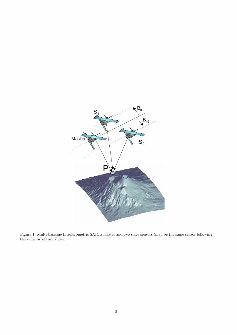
Let us refer to the multibaseline geometry in Fig. 1, an extension of the conventional SAR Interferometry [12, 13]to the multi channel case. In the figure, the target P corresponds to a distributed scatterer, that is imagedusing three different positions. Let us define the normal baseline Bn as the distance between the master and theslave’s track, measured normal to the slant range, azimuth plane. In the case shown in the picture, we couldcompute up to three interferograms, as the Hermitian products between two images, all of them coregistered inthe same master reference. The contribute of the target P to the interferogram’s phase would be proportionalto the travel path difference between the two acquisitions

∆ϕ =4π

λ(Rs(P )−RM (P )) (1)

where RS and RM are respectively the slave-target and the master-target travel path. Eventually we approxi-mate the interferogram phase as a slow varying linear term[14]:

φ(t) = −f0∆θ

tan(θ − α(t))t (2)

≈ −f0Bn

R0 tan(θ − α(t))t (3)

α(t) being the local slope (range-varying), R0 the closest approach, f0 the carrier frequency, and ∆θ the lookangle difference. The approximation in (3) holds for range intervals narrow enough to assume ∆θ constant.

In (3) the interferogram phase scales linearly both with the Bn and with f0, therefore we may get differentinterferograms either by exploiting multi-baseline or multi-frequency systems. In this paper we will refer to bothcases as ”multi-channel”, however we will address mostly the multi baseline case, that is much more commonin spaceborne SARs.

Let us assume to have N channels, including one master and (N − 1) slave images, and M samples (rangebins) from each acquisition. Following reference [11], we express each single acquisition as a filtered version ofthe wide-band reflectivity:

yi(P (t)) = γ(t) exp (jφ(t)) + wi(t) (4)

We limit our study to the 1D case, as the slant range, or fast-time, t, is the direction mostly affected by phasealiasing and baseline decorrelation due to the geometric deformations in the ground-to-range mapping [15]. In(4), γ is the source reflectivity, yi the focused signal of the i-th acquisition, and wi a noise source that cumulatesall the decorrelation terms [16].

In order to proper process the data, we need to up-sample the received signal, so that the final range samplingwould accommodate for all the possible spectral shifts, e.g. by computing (3) for the largest baseline. After upsampling each channel in 4, we end up in a discrete-time model that can be expressed by the following vectorformulation [11], represented schematically in Fig. 2:

yi = FiΦiγ + wi = Hiγ + wi (5)

where we assume bold notation for matrixes and vectors. In particular, we assume that the impulse responseon each channel is of length L, and we to have N channels, and M samples out of each channel. We require thenM+L-1 samples of the source. The vectors and matrixes involved in (5) are the following:

2

P

Bn1

Bn2

Master

S1

S2

Figure 1: Multi-baseline Interferometric SAR: a master and two slave sensors (may be the same sensor followingthe same orbit) are shown.

3

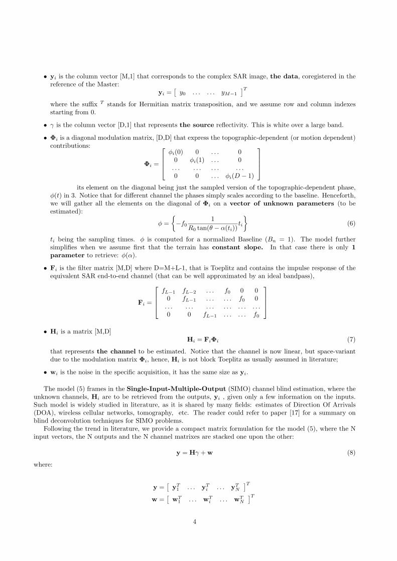
• yi is the column vector [M,1] that corresponds to the complex SAR image, the data, coregistered in thereference of the Master:

yi =[

y0 . . . . . . yM−1

]Twhere the suffix T stands for Hermitian matrix transposition, and we assume row and column indexesstarting from 0.

• γ is the column vector [D,1] that represents the source reflectivity. This is white over a large band.

• Φi is a diagonal modulation matrix, [D,D] that express the topographic-dependent (or motion dependent)contributions:

Φi =

φi(0) 0 . . . 0

0 φi(1) . . . 0. . . . . . . . . . . .0 0 . . . φi(D − 1)

its element on the diagonal being just the sampled version of the topographic-dependent phase,

φ(t) in 3. Notice that for different channel the phases simply scales according to the baseline. Henceforth,we will gather all the elements on the diagonal of Φi on a vector of unknown parameters (to beestimated):

φ =−f0

1R0 tan(θ − α(ti))

ti

(6)

ti being the sampling times. φ is computed for a normalized Baseline (Bn = 1). The model furthersimplifies when we assume first that the terrain has constant slope. In that case there is only 1parameter to retrieve: φ(α).

• Fi is the filter matrix [M,D] where D=M+L-1, that is Toeplitz and contains the impulse response of theequivalent SAR end-to-end channel (that can be well approximated by an ideal bandpass),

Fi =

fL−1 fL−2 . . . f0 0 0

0 fL−1 . . . . . . f0 0. . . . . . . . . . . . . . . . . .0 0 fL−1 . . . . . . f0

• Hi is a matrix [M,D]

Hi = FiΦi (7)

that represents the channel to be estimated. Notice that the channel is now linear, but space-variantdue to the modulation matrix Φi, hence, Hi is not block Toeplitz as usually assumed in literature;

• wi is the noise in the specific acquisition, it has the same size as yi.

The model (5) frames in the Single-Input-Multiple-Output (SIMO) channel blind estimation, where theunknown channels, Hi are to be retrieved from the outputs, yi , given only a few information on the inputs.Such model is widely studied in literature, as it is shared by many fields: estimates of Direction Of Arrivals(DOA), wireless cellular networks, tomography, etc. The reader could refer to paper [17] for a summary onblind deconvolution techniques for SIMO problems.

Following the trend in literature, we provide a compact matrix formulation for the model (5), where the Ninput vectors, the N outputs and the N channel matrixes are stacked one upon the other:

y = Hγ + w (8)

where:

y =[

yT1 . . . yT

i . . . yTN

]Tw =

[wT

1 . . . wTi . . . wT

N

]T4

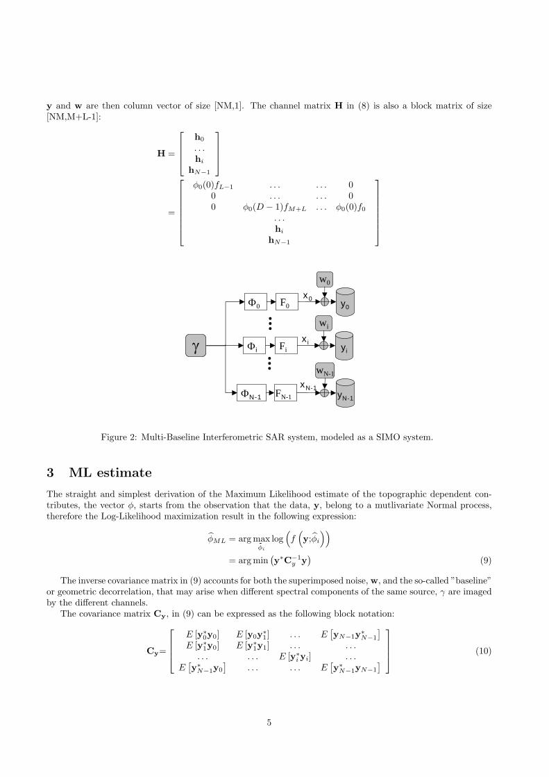
y and w are then column vector of size [NM,1]. The channel matrix H in (8) is also a block matrix of size[NM,M+L-1]:

H =

h0

. . .hi

hN−1

=

φ0(0)fL−1 . . . . . . 0

0 . . . . . . 00 φ0(D − 1)fM+L . . . φ0(0)f0

. . .hi

hN−1

Φ0 F0

γ Φi Fi...ΦN-1 FN-1

y0

w0

yi

wi...

yN-1

wN-1

x0

xN-1

xi

Figure 2: Multi-Baseline Interferometric SAR system, modeled as a SIMO system.

3 ML estimate

The straight and simplest derivation of the Maximum Likelihood estimate of the topographic dependent con-tributes, the vector φ, starts from the observation that the data, y, belong to a mutlivariate Normal process,therefore the Log-Likelihood maximization result in the following expression:

φML = arg maxbφi

log(f(y;φi

))= arg min

(y∗C−1

y y)

(9)

The inverse covariance matrix in (9) accounts for both the superimposed noise, w, and the so-called ”baseline”or geometric decorrelation, that may arise when different spectral components of the same source, γ are imagedby the different channels.

The covariance matrix Cy, in (9) can be expressed as the following block notation:

Cy=

E [y∗0y0] E [y0y∗1] . . . E

[yN−1y∗N−1

]E [y∗1y0] E [y∗1y1] . . . . . .

. . . . . . E [y∗i yi] . . .E[y∗N−1y0

]. . . . . . E

[y∗N−1yN−1

] (10)

5

Each block can be estimated basing on the model (8) and (7) (see Fig. 2):

E [y∗i yi] = F∗i φ

∗i CγφiFi + Cwi (11)

E [y∗i yj ] =i 6=j

F∗i φ

∗i CγφjFj + E [wiwj ] (12)

= F∗i φ

∗i CγφjFj (13)

where Cwi is the covariance matrix of the noise term in the i-th channel, and where we have introduced thedefinition:

Cγ = E [γγ∗]

The need of the covariance matrix inversion makes the ML estimator unfeasible, but for simple cases requiringone or two parameters to be retrieved and involving few images. The most interesting case could be the estimateof slopes basing on a very local scale (a few pixels) in a conventional two channel interferometric system [18].

4 DML estimate

The Deterministic Maximum Likelihood (DML) method approaches the same problem by including in the vectorof parameters the samples of the source, γ [17], [19]. This choice provides a simpler solution, at the price ofincreasing the number of parameters to be estimated and potentially worsening the accuracy of the estimates.The problem is linear in both the channel and the sources, therefore we can cascade the optimizations withrespect to γ and φ:

φDML, γ

= arg minbφ

(minbγ

((y −Hγ)∗ C−1 (y −Hγ)

))(14)

where C−1 is the noise covariance matrix. Eventually we define the SIMO channel covariance:

RH = H∗C−1H = Φ∗F∗C−1FΦ (15)

We first minimize with respect to the sources:

minbγ

(y∗C−1γH + H∗γ∗C−1y −H∗γ∗C−1γH

)(16)

that leads to the solution:

γDML = R†HH∗C−1y = R†

HΦ∗F∗C−1y (17)

where R†H is the pseudo-inverse of the channel covariance. We do not need the explicit computation of γDML

if we are not interested, we just need to substitute its expression back into (14), to retrieve the estimate of φ:

φDML = max (y∗PHy) (18)

where PH is a projector in the norm of the channel H :

PH = C−1HR†HH∗C−1 (19)

= C−1FΦR†HΦ∗F∗C−1 (20)

.The DML estimate φDML appears as complex as the ML approach in (18), as one matrix inversion is

required to compute R†H at each iteration. However, a sub-optimal implementation is known as the Two-Step

ML (TSML), introduced by Hua in [19]. This approach makes a first iteration by assuming that the channelcovariance matrix is diagonal: R†

H = I. In that case the DML estimate would be

φDMLI = maxbφ

(y∗C−1FΦΦ∗F∗C−1y

)(21)

6

this leads to an estimate of φDMLI that is shown to be optimal as for SNR→∞ [19]. An approximate value ofR†

H is computed by combining (15) with the first-step estimate φDMLI in (21). Thereafter, the final estimateφDML is retrieved from (20).

In a similar way, in papers [10] and [11] a preliminary information of the geometry and the topography wasused to derive the proper whitening operator.

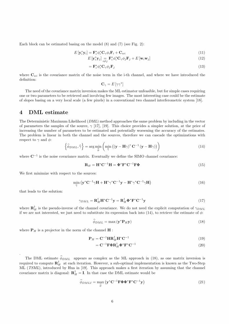
5 Single baseline interferometry

Let us compare the two estimates of the topographic-dependent phase in the simplest case, the single baselineinterferometry. The model of the Interferometric SAR channel is represented in Fig. 3.a, whereas Fig. 3.bdraws the linear estimate of the parameters φ. The linear estimate is justified by the Normal statistics of bothsources and noise. We will however derive it, and show that, by a proper selection of the coefficients, the samescheme in Fig. 3.b can represent either the ML or the DML approach. In the figure, we have conventionallyattributed half of the interferometric phase, Φ−1/2, to the master, and the other half to the slave. Furthermore,we changed the conventional SIMO model (see Fig. 2) by moving the noise contribution in front of the blocks F(that represents the SAR acquisition and focusing overall transfer function). This choice is closer to the actualSAR acquisition. However, the two models are both correct, provided that the proper noise covariance matrixis used.

Φ1 F1 y1

Φ2 F2 y2

γ

Master

H1

G21 y2|1

y1|2

H2

Slave

Slave synthesis

Master synthesis

w2

w1

(a) (b)Δφ

G12

y2|1

y1|2

Figure 3: Single baseline interferometry: (a) the acquisition model, and (b) the linear estimator of the interfer-ometric phase. This estimator applies for both the ML and the DML technique.

5.1 DML estimate

Let us first find a suitable approximation of the inverse of the noise covariance matrix involved in the DMLestimate (14). Let us assume the same kernel for both channels, F0 = F1 = F that is usually the case inmulti-pass interferometry. The model in Fig. 3.a allows us to express the noise covariance as the followingKronecker product:

C =[

σ20 00 σ2

1

]⊗RF

where σ20 and σ2

1 are the noise variances in the two channels, and RF expresses the channel cross-correlation.Eventually we take advantage of the inversion expression for Kronecker products:

(A⊗B)−1 = A−1 ⊗B−1

7

that leads to the inverse of the channel covariance matrix:

C−1=[

σ−20 00 σ−2

1

]⊗R−1

F

=[

σ−20 R−1

F 00 σ−2

1 R−1F

]=[

C00 00 C11

](22)

Having expressed the inverse noise covariance as a block matrix, with two non null blocks, we may write theDML estimator, (18), (20), as follows:

M = y∗0C00H0R†HH∗

0C00y0 + y∗1C11H1R†HH∗

1C11y1 (23)

+ y∗0C00H0R†HH∗

1C11y1 + y∗1C11H1R†HH∗

0C00y0 (24)

where the channel covariance matrix is:

RH = H∗C−1H = σ−20 H

∗0R

−1F H0 + σ−2

1 H∗1R

−1F H1 (25)

5.1.1 TSML: Fist Step

Let us now follow the TSML approach by providing a first estimate of φ by assuming R†H = I. The two addends

in (23), involve auto-correlations of each of outputs separately, therefore are blind to the interferometric phasesand can be dropped. In fact the following expression holds for both i = 0 and i = 1:

y∗i HiH∗i yi = y∗i FiΦ−1/2Φ1/2F∗

i yi = y∗i FiF∗i yi

that no longer depends in φ. The first step of the DML is then the maximization of the summation in (24):

M = y∗0C00H0H∗1C11y1 + y∗1C11H1H∗

0C00y0 (26)= 2Re(y∗1C11H1H∗

0C00y0) (27)= 2Re(s∗1s0) (28)

According to the scheme in Fig. 3.b, we interpret the DML (1st step) as the maximization of the cross-energyof two signals, s1 and s0 obtained by applying the kernels:

G0 = H∗0C00 = σ−2

0 Φ1/2

F∗0R

−1F (29)

G1 = H∗1C11 = σ−2

1 Φ−1/2

F∗1R

−1F (30)

to the outputs y0 and y1.We may assume that the channel kernels have no phase bias, i.e. F0 and F1 are Toeplitz, hence the products

P0= F∗0R

−1F and P1= F∗

1R−1F will still be two Toeplitz matrixes, P0 and P1. We can now derive the DML

estimate form (27):

φDMLI = arg max (Re (y∗1P1ΦP∗0y0))

= arg max

(Re∑

n

exp(jφn)y∗1P∗1P0y0

)(31)

that is maximized by imposing:

φDMLI(n) = arg(y∗1(n)y0(n)) = arg I10 (32)

I10 being the complex interferogram. Not surprisingly, the first step of the DML corresponds to the usualapproach, that retrieves the phase, as the argument of the complex interferogram. Notice that this approach is

8

optimal as SNR→∞.

In the case of constant sloped terrain (31), would be the Fourier Transform of the complex interferogram,evaluated at the frequency ∆φn/(2π), and the maximization of the likelihood corresponds to the conventionalperiodogram-based frequency estimation..

5.1.2 TS-DML: Second Step

The second step is performed by maximizing the likelihood:

M = 2 Re(y∗1C11H1R†HH∗

0C00y0) (33)

where R†H is the pseudo inverse of the channel autocorrelation (25) computed basing on the parameter φDMLI

from (32). Apart from this term, we would get the same result as in (32). The linear estimator in Fig. 3.b stillholds, but we now need to modify (29,30) by including R†1/2

H to both terms.In order to have a reasonable idea of the role played by the term R†

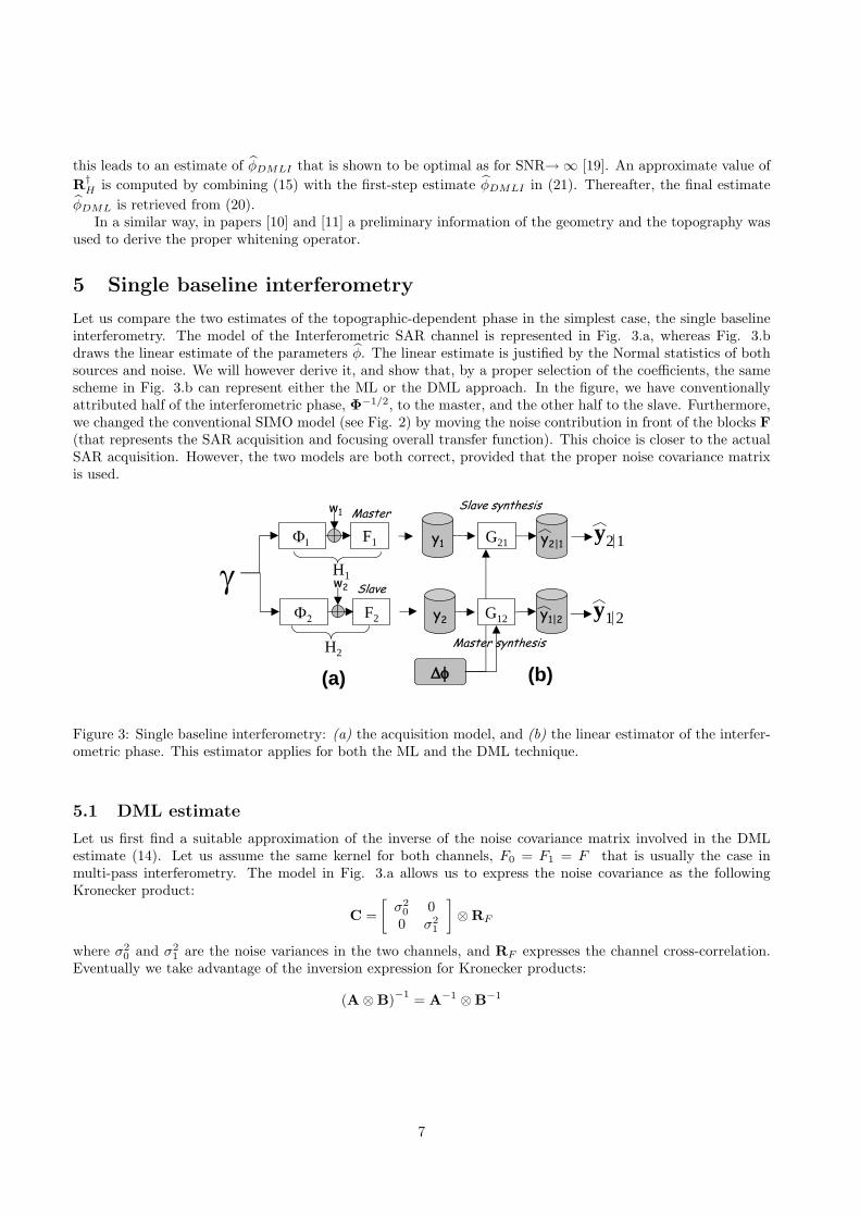
H , let us assume (1) a constant slopedterrain, and (2) a stationary case. The system can now be studied as in terms of linear, time variant convolutions.The forward model in Fig. 3.a becomes:

y0(t) = γ(t) · exp(−jΩt) + w0(t) ∗ f0(t) (34)y1(t) = γ(t) · exp(jΩt) + w1(t) ∗ f1(t) (35)

that is then sampled at a frequency consistent with the bandwidth of the on-board filters, f0(t) and f1(t). Thefrequency domain representation of the spectra Y0(f) and Y1(f) are shown in Fig. 4 (the two upper plots).

Figure 4: Single baseline model in the frequency domain, for a constant sloped terrain. Notice the spectral shift,∆f , that depends on the local slope and the baseline.

We have assumed ideal boxcar bandpass spectra, centered on the carrier frequency. Under this assumption,the autocorrelation of the two channels will have the same bandpass shape, then we will approximate the inversenoise covariance (22) as follows:

C−1=[

σ−20 F0 00 σ−2

1 F1

](36)

9

Eventually, we get from (25):

RH = σ−20

(Φ1/2F∗

0

)F0F0

(F∗

0Φ−1/2

)+ σ−2

1

(Φ−1/2F∗

1

)F1F1

(F∗

1Φ1/2)

(37)

In the constant slope case, the inverse kernel R†H will perform a ”whitening”, e.g. the equalization in the

frequency domain, shown in Fig. 4, last plot. Even if in this specific case, we do not expect any differencewith the result achieved at the first step, this equalization would be effective in the Multi-Baseline (SIMO)environment, when many channels could contribute to the same spectrum.

5.2 ML estimate

Let us now find a suitable approximation for the ML estimate in (9). We first introduce a matrix in thecomplementary space of the signal covariance: G = I−Cy, the ML is now the following maximization

φML = arg max(y∗G−1y

)(38)

The inverse of the matrix G can be expressed as the block matrix:

G−1=[

G00 G01

G10 G11

]The ML estimate is then:

Φ =arg max (y∗0G00y0 + y∗1G01y0 + y∗0G10y1 + y∗1G11y1)= arg max (y∗0G00y0 + 2 Re (y∗1G01y0) + y∗1G11y1) (39)

The likelihood to be maximized is similar in topology (but non identical in weights) to the one in the DMLestimate, (23).

Instead of inverting the covariance matrix, we can directly derive the ML by finding the weights and Gij

that maximizes (39). We observe that the solution is already known in the literature, in fact, in [11] the linearmodel in Fig. 3.b:

s0 = G0y0 and s1 = G1y1 (40)

was exploited to minimize the squared error:

minG0,G1

[‖y1 −G0y0‖2 + ‖y0 −G1y1‖2

](41)

= max[−y∗0G

∗0G0y0 + y∗1G0y0 + y∗0G0y1

−y∗1G∗1G1y1 + y∗0G1y1 + y∗1G1y0

]that is formally equivalent to the likelihood (39). The minimization of (41) gives the result (see [11]) :

G0 '1

1 + SNR−1F1Φ1/2F∗

0 (F0F∗0) † (42)

' 11 + SNR−1

0

F1Φ1/2F∗0 (43)

G1 =1

1 + SNR−11

F0Φ1/2F∗1 (44)

where SNR−10 , SNR−1

1 are the ratio between the noise power (in the signal bandwidth) and the signal powerin each channel, and (42) is an approximation that gives almost the same results if the channels F1, F0 haveflat frequency response in their pass-band.

5.3 Deterministic and statistic likelihood

10

We have just shown that both DML and ML estimates are performed by means of linear kernels, whose expres-sions (29,30) and (43,44) appears quite similar. The most outstanding difference is due to the inclusion, in theML case, of the weighting factor:

ρ =1

1 + SNR−10

11 + SNR−1

1

that corresponds to the definition of the coherence of the interferometric pair [16]. The channel decorrelation isnot handled in the DML approach, as this one regards the sources as set of parameters to be estimated ratherthan the realization of a statistical process.

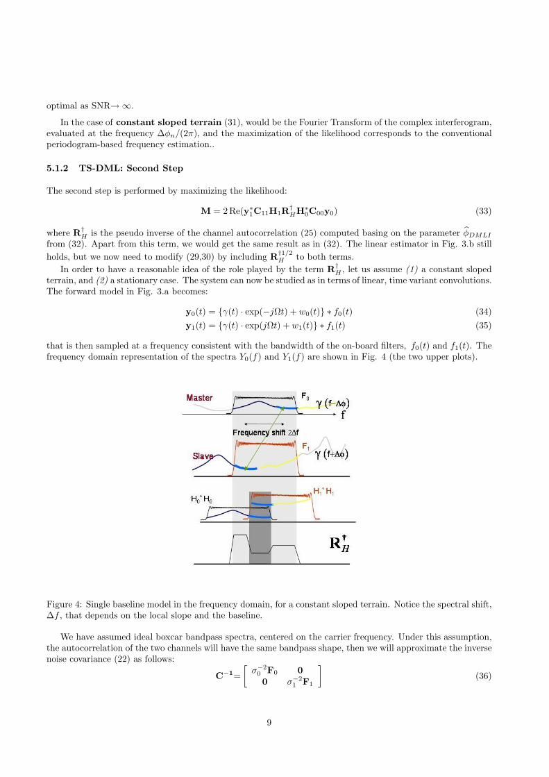
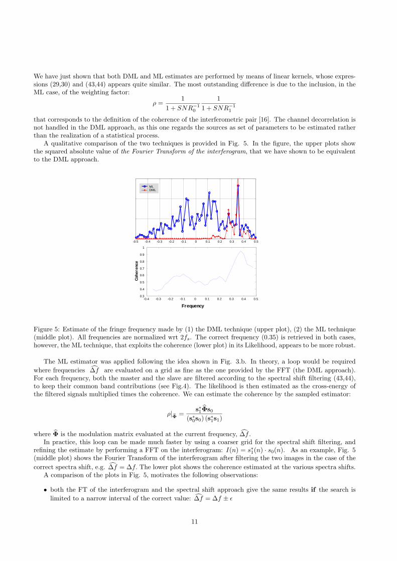
A qualitative comparison of the two techniques is provided in Fig. 5. In the figure, the upper plots showthe squared absolute value of the Fourier Transform of the interferogram, that we have shown to be equivalentto the DML approach.

-0.5 -0.4 -0.3 -0.2 -0.1 0 0.1 0.2 0.3 0.4 0.5

MLDML

0.3

0.4

0.5

0.6

0.7

0.8

0.9

1

-0.4 -0.3 -0.2 -0.1 0 0.1 0.2 0.3 0.4 0.5

Cohe

renc

e

Frequency

Figure 5: Estimate of the fringe frequency made by (1) the DML technique (upper plot), (2) the ML technique(middle plot). All frequencies are normalized wrt 2fs. The correct frequency (0.35) is retrieved in both cases,however, the ML technique, that exploits the coherence (lower plot) in its Likelihood, appears to be more robust.

The ML estimator was applied following the idea shown in Fig. 3.b. In theory, a loop would be requiredwhere frequencies ∆f are evaluated on a grid as fine as the one provided by the FFT (the DML approach).For each frequency, both the master and the slave are filtered according to the spectral shift filtering (43,44),to keep their common band contributions (see Fig.4). The likelihood is then estimated as the cross-energy ofthe filtered signals multiplied times the coherence. We can estimate the coherence by the sampled estimator:

ρ|bΦ =

s∗1Φs0

(s∗0s0) (s∗1s1)

where Φ is the modulation matrix evaluated at the current frequency, ∆f .In practice, this loop can be made much faster by using a coarser grid for the spectral shift filtering, and

refining the estimate by performing a FFT on the interferogram: I(n) = s∗1(n) · s0(n). As an example, Fig. 5(middle plot) shows the Fourier Transform of the interferogram after filtering the two images in the case of thecorrect spectra shift, e.g. ∆f = ∆f. The lower plot shows the coherence estimated at the various spectra shifts.

A comparison of the plots in Fig. 5, motivates the following observations:

• both the FT of the interferogram and the spectral shift approach give the same results if the search islimited to a narrow interval of the correct value: ∆f = ∆f ± ε

11

• the spectral shift approach is more robust due to the use of the coherence in the likelihood.

We then notice that the inclusion of coherence in the likelihood allows to better discriminate which of thespectral peaks in Fig. 3 is the ”true” one, whereas the coherence peak is too flat to provide an improvement inthe fine estimate ∆f . We once again remind that the weakness of the DML is due to the higher number ofparameters to be estimated. We than expect that, at the highest SNR, and for large estimation windows, thetwo techniques would provide the same results, whereas different results would be achieved at the low SNR.

A practical idea of this limit value is provided in Fig. 5. The figure shows the standard deviation of theestimate of ∆f as a function of the coherence and for different window sizes, L, achieved by means of a Monte-Carlo simulation, with the DML approach. For high coherence/SNR, all the estimates gives the same accuracy,once that they are scaled times the square root of the window length,

√L. However, for the low SNR, the

performances drops and the estimated frequency is biased towards 0, a fact well known in literature [20]. Inthat case, the ML estimate would get significant improvements.

0.2 0.3 0.4 0.5 0.6 0.7 0.8 0.9 1

100

Coherence

σ ∆ f

L=5

L =10

L=20

L=50

L=100

Figure 6: Standard deviation of the frequency estimate made by the DML approach, for different size of theestimation window, as a function of the coherence. Notice the threshold behavior for coherences ranging form0.35 (L=5) to 0.95 (L=100).

6 Multi-Baseline Slope Estimate

The multi-baseline case is more complicated than the single baseline case. In fact, although we are still able toextend the DML approach, we have no closed form solution for the ML in (9) that would avoid the inversion ofthe covariance matrix. We than propose a straight extension of (26), by simply adding coherence-based weightsto get close to the ML results. We need then to maximize the following figure of merit:

φ = argmaxN−1∑j=0

N−1∑i=0

ρij(φ)y∗i Gijyj (45)

where the weights are computed basing on (29), and assuming the noiseless case (as we already accounts fornoise with the coherence):

Gi = Φ1/2ij F∗

i

The diagonal matrixes Φij keeps the elements of φ in (6) properly scaled by the baseline of the pair i, j. Themaximum is then found by iterating for all the values of the normalized frequency shift, ∆f. Furthermore theco-channel terms (for i = j), are useless for the estimate of the phase term φ, and they can be dropped fromthe summation (45). This can be shown by writing the Fourier Transform of the SAR channel (34):

Yi(f) = Γ(f) ∗ δ(f −∆f(α(t))) · Fi(f)= Γ(f −∆f) · Fi(f) (46)

12

where ∆f(α(t) is the spectral shift, that depends on the slope. The power spectrum of the reflectivity,E[|Γ(f)|2

], is white over a large bandwith, therefore the power spectrum of the output, E

[|Yi(f)|2

]car-

ries no information on ∆f. Nor we can retrieve any information from the phase of Yi(f), as the sources areGaussian.

Having dropped the co-channel contribution, (45) reduces to the summation of averaged interferograms(i 6= j):

ρij(φ)y∗i Gijyj

Attention should be taken in order to exclude, at each value of the parameter ∆f, the contributions that wouldbe aliased. The constraint we have to impose is indeed more stringent, as we want to avoid biasing in thecoherence estimate. Given a spectral shift ∆f, the common bandwidth would be Bc = B −∆f , where Bi isthe SAR channel bandwidth. If we exploit patches on the ground of L pixels, sampled at a rate fs, the numberof effectively independent samples would be:

Ni = LBc

fs=

L

fs

(Bmax − f0

Bn

R0 tan(θ − α)

)and we need Ni 1 to avoid biasing of the coherence estimate ρij → 1.

Finally, we remark that in the straight extension from the single baseline, (42), to the MB case (45), wehave not accounted for a spectral equalization like the one provided by the operator R†

H (see Fig. 4), howeverthis topic could be a subject for future analysis.

6.1 Experimental results

The proposed MB InSAR estimation algorithm has been tested first with synthetic and then with real data.The estimation algorithm has been applied with respect to the pixel-to-pixel phase differences in range, in orderto remove any potential problem coming from tropospheric phase screen or other unknown phase offsets. Weselected a 5 samples window length as a compromise between accuracy and resolution. The algorithms testedwere based on the combination (45) in the two following implementations:

- DML unweighed,- ML, including the spectral shift filtering and weights derived by the a-posteriori estimate of the coherence.In presenting the results we have also added a single interferogram image for comparison.

6.2 Results from simulations

A set of 6 images was simulated by assuming the parameters of ENVISAT-ERS systems and the topography ofMt. Vesuvius. The baselines were chosen to cover a range of 1000 m with uniform sampling but taking care toavoid periodicity. The baseline vector is [-470 -310 100 +330 +580] m with respect to the master. We did notadd any further decorrelation, apart from the unavoidable baseline decorrelation. Having the perfect knowledgeof the topography, we could perform an accurate evaluation of the estimator performances for different slopes.These results are shown in Fig. 7. Fig. 7.a maps the local phase gradient in range expressed in radians andmeasured on the theoretical unwrapped phase that would come from the 470 m baseline interferogram.The othergraphics in the same figure show the natural logartihm of the counts of measured slopes with respect to thetrue slope, a sort of scatter-plot. The estimates are based on a single interferogram, in Fig. 7.(b), on the DMLestimator, Fig. 7.(c) and on the proposed ML-derived estimator, Fig. 7.(d).

The single interferogram is clearly limited in the trade-offs between altimetric resolution and phase aliasing.In the case shown we selected a small baseline (100 m), nonetheless there is a sensible loss of the contributioncoming from the higher slopes. We also notice the large variance, due to the fact that only two images wereexploited instead of the five available.

The DML estimate, in Fig. 7.(c) is almost useless, due to the strong biasing of the estimate, as discussed insection 5.3. On the other hand, the estimate achieved by the proposed technique, shown in Fig. 7.d, provides thehigher accuracy for the low values of the gradient, due to the cooperation of all the images, and the capabilityto solve the highest gradient with no aliasing, due to the combinations with the lowest baselines.

13

−3

−2.5

−2

−1.5

−1

−0.5

0

∆ φ

∆ φ e

−8 −6 −4 −2 0−8

−7

−6

−5

−4

−3

−2

−1

0

1

2

−6

−4

−2

0

2

4

6

8

10

(a) (b)

∆ φ

∆ φ e

−8 −6 −4 −2 0−8

−7

−6

−5

−4

−3

−2

−1

0

1

2

−6

−4

−2

0

2

4

6

8

∆ φ

∆ φ e

−8 −6 −4 −2 0−8

−7

−6

−5

−4

−3

−2

−1

0

1

2

−6

−4

−2

0

2

4

6

8

10

(c) (d)

Figure 7: (a) Phase gradient ∆φ, along slant range, of a 500 m interferogram on Mt. Vesuvius. (b-d) Scatterdiagram of ∆φ estimated versus true value for different estimator. (b) single-baseline interferogram, (c) MBbased on the unweighted combination , (d) MB achieved by both exploiting coherence weights and spectral shiftfiltering.

14

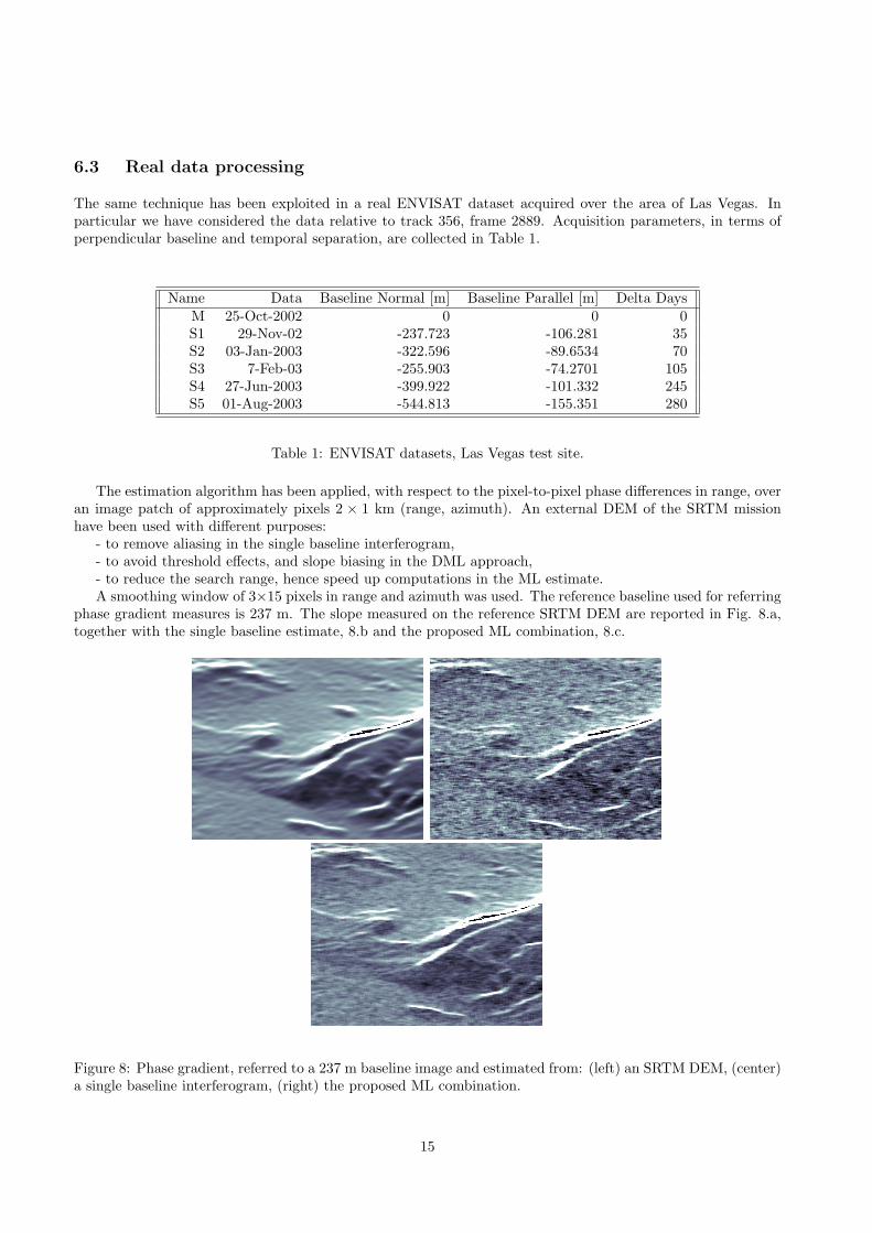
6.3 Real data processing

The same technique has been exploited in a real ENVISAT dataset acquired over the area of Las Vegas. Inparticular we have considered the data relative to track 356, frame 2889. Acquisition parameters, in terms ofperpendicular baseline and temporal separation, are collected in Table 1.

Name Data Baseline Normal [m] Baseline Parallel [m] Delta DaysM 25-Oct-2002 0 0 0S1 29-Nov-02 -237.723 -106.281 35S2 03-Jan-2003 -322.596 -89.6534 70S3 7-Feb-03 -255.903 -74.2701 105S4 27-Jun-2003 -399.922 -101.332 245S5 01-Aug-2003 -544.813 -155.351 280

Table 1: ENVISAT datasets, Las Vegas test site.

The estimation algorithm has been applied, with respect to the pixel-to-pixel phase differences in range, overan image patch of approximately pixels 2 × 1 km (range, azimuth). An external DEM of the SRTM missionhave been used with different purposes:

- to remove aliasing in the single baseline interferogram,- to avoid threshold effects, and slope biasing in the DML approach,- to reduce the search range, hence speed up computations in the ML estimate.A smoothing window of 3×15 pixels in range and azimuth was used. The reference baseline used for referring

phase gradient measures is 237 m. The slope measured on the reference SRTM DEM are reported in Fig. 8.a,together with the single baseline estimate, 8.b and the proposed ML combination, 8.c.

Figure 8: Phase gradient, referred to a 237 m baseline image and estimated from: (left) an SRTM DEM, (center)a single baseline interferogram, (right) the proposed ML combination.

15

Here again we find the same features as in the simulated results, although the altimetric resolution is lessevident due to the smaller baseline span. Notice the ML combination gets result similar to the SRTM DEM forboth robustness with respect to ambiguity and the accuracy.

6.4 Acknowledgments

The author would like to thank the Italian Space Agency for sponsoring of the work (ASI contract I/R/169/02Multiple pass SAR Interferometry for very accurate Earth modeling). Thanks also to Dr. Ing. F. De Zan forthe proficuous discussions on the statistic of the ML approach.

7 Conclusions

In the paper we have studied two different Maximum Likelihood techniques to provide estimates of the terraintopography in a Multi-Baseline SAR interferometric case, namely the Deterministic ML and the statistic ML.The first approach includes the sources in the vector of parameters, and thus it is less robust than the second(particularly when few samples are available). However, its quite efficient and suited for applications when apreliminary knowledge of the slope exists. The second estimator, the ML approach, was derived as an extensionof the MB case the exact ML estimated for conventional interferometry. A preliminary validation of thistechnique has demonstrated the capabilities of solving aliasing for the higher slopes, due to the use of thelower baselines, and to attain at the same time the high altimetric resolution that would come from the higherbaselines. The major limit of the technique, the computational complexity, leaves open opportunities for furtherresearches.

References

[1] F. K. Li and R. M. Goldstein, “Studies of multibaseline spaceborne interferometric synthetic apertureradars,” IEEE Transactions on Geoscience and Remote Sensing, vol. 28, no. 1, pp. 88–97, Jan. 1990.

[2] D. Massonnet, H. Vadon, and M. Rossi, “Reduction of the need for phase unwrapping in radar interferom-etry,” IEEE Transactions on Geoscience and Remote Sensing, vol. 34, no. 2, pp. 489–497, Mar. 1996.

[3] R. Lanari, G. Fornaro, D. Riccio, M. Migliaccio, K. P. Papathanassiou, J. ao R Moreira, M. Schwabisch,L. Dutra, G. Puglisi, G. Franceschetti, and M. Coltelli, “Generation of digital elevation models by us-ing SIR-C/X-SAR multifrequency two-pass interferometry: The Etna case study,” IEEE Transactions onGeoscience and Remote Sensing, vol. 34, no. 5, pp. 1097–1114, Sept. 1996.

[4] A. Ferretti, C. Prati, F. Rocca, and A. Monti Guarnieri, “Multibaseline SAR interferometry forautomatic DEM reconstruction,” in Third ERS Symposium—Space at the Service of our Environment,Florence, Italy, 17–21 March 1997, ser. ESA SP-414, 1997, pp. 1809–1820. [Online]. Available:http://earth1.esrin.esa.it/florence/data/ferretti/index.html

[5] F. Lombardini, “Optimal absolute phase retrieval in three-element SAR interferometry,” Electronics Letters,vol. 34, no. 5, pp. 1522–1524, July 1998.

[6] V. Pascazio and G. Schirinzi, “Estimation of terrain elevation by multifrequency interferometric wide bandSAR data,” IEEE Signal Processing Lett., vol. 8, pp. 7–9, 2001.

[7] A. Ferretti, C. Prati, and F. Rocca, “Permanent scatterers in SAR interferometry,” IEEE Transactions onGeoscience and Remote Sensing, vol. 39, no. 1, pp. 8–20, Jan. 2001.

[8] F. Gatelli, A. Monti Guarnieri, F. Parizzi, P. Pasquali, C. Prati, and F. Rocca, “The wavenumber shift inSAR interferometry,” IEEE Transactions on Geoscience and Remote Sensing, vol. 32, no. 4, pp. 855–865,July 1994.

[9] G. W. Davidson and R. Bamler, “Multiresolution phase unwrapping for SAR interferometry,” IEEE Trans-actions on Geoscience and Remote Sensing, vol. 37, no. 1, pp. 163–174, Jan. 1999.

16

[10] A. M. Guarnieri and F. Rocca, “Combination of low- and high-resolution SAR images for differentialinterferometry,” IEEE Transactions on Geoscience and Remote Sensing, vol. 37, no. 4, pp. 2035–2049, July1999.

[11] G. Fornarno and A. M. Guarnieri, “Minimum mean square error space-varying filtering of interferometricSAR data,” IEEE Transactions on Geoscience and Remote Sensing, vol. 40, no. 1, pp. 11–21, July 2002.

[12] R. Bamler and P. Hartl, “Synthetic aperture radar interferometry,” Inverse Problems, vol. 14, pp. R1–R54,1998.

[13] P. Rosen, S. Hensley, I. R. Joughin, F. K. Li, S. Madsen, E. Rodrıguez, and R. Goldstein, “Syntheticaperture radar interferometry,” Proceedings of the IEEE, vol. 88, no. 3, pp. 333–382, Mar. 2000.

[14] A. M. Guarnieri, “SAR interferometry and statistical topography,” IEEE Trans. Geosc. Remote Sens.,vol. 40, no. 12, pp. 2567–2581, Dec. 2002.

[15] H. A. Zebker and J. Villasenor, “Decorrelation in interferometric radar echoes,” IEEE Transactions onGeoscience and Remote Sensing, vol. 30, no. 5, pp. 950–959, sept 1992.

[16] D. Just and R. Bamler, “Phase statistics of interferograms with applications to synthetic aperture radar,”Applied Optics, vol. 33, no. 20, pp. 4361–4368, 1994.

[17] L. Tong and S. Perreau, “Multichannel blind identification: From subspace to maximum likelihood meth-ods,” Proc. IEEE, vol. 86, no. 10, pp. 1951–1968, Oct. 1998.

[18] F. De-Zan, “Stima ottima della fase nell’interferometria SAR,” Ph.D. dissertation, Politecnico di Milano,July 2004.

[19] Y. Hua, “Fast maximum likelihood for blind identification of multiple FIR channels,” IEEE Transactionson Signal Processing, vol. 44, pp. 661–672, Mar. 1996.

[20] R. Bamler, N. Adam, G. W. Davidson, and D. Just, “Noise-induced slope distortion in 2-d phase unwrap-ping by linear estimators with application to SAR interferometry,” IEEE Transactions on Geoscience andRemote Sensing, vol. 36, no. 3, pp. 913–921, May 1998.

17