characterization and anomalous diffusion analysis of a

Air Force Institute of TechnologyAFIT Scholar

Theses and Dissertations Student Graduate Works

3-21-2019

Characterization and Anomalous DiffusionAnalysis of a 100w Low Power Annular Hall EffectThrusterMegan N. Maikell

Follow this and additional works at: https://scholar.afit.edu/etd

Part of the Propulsion and Power Commons

This Thesis is brought to you for free and open access by the Student Graduate Works at AFIT Scholar. It has been accepted for inclusion in Theses andDissertations by an authorized administrator of AFIT Scholar. For more information, please contact [email protected].

Recommended CitationMaikell, Megan N., "Characterization and Anomalous Diffusion Analysis of a 100w Low Power Annular Hall Effect Thruster" (2019).Theses and Dissertations. 2226.https://scholar.afit.edu/etd/2226

https://scholar.afit.edu?utm_source=scholar.afit.edu%2Fetd%2F2226&utm_medium=PDF&utm_campaign=PDFCoverPages

https://scholar.afit.edu/etd?utm_source=scholar.afit.edu%2Fetd%2F2226&utm_medium=PDF&utm_campaign=PDFCoverPages

https://scholar.afit.edu/graduate_works?utm_source=scholar.afit.edu%2Fetd%2F2226&utm_medium=PDF&utm_campaign=PDFCoverPages

https://scholar.afit.edu/etd?utm_source=scholar.afit.edu%2Fetd%2F2226&utm_medium=PDF&utm_campaign=PDFCoverPages

http://network.bepress.com/hgg/discipline/225?utm_source=scholar.afit.edu%2Fetd%2F2226&utm_medium=PDF&utm_campaign=PDFCoverPages

https://scholar.afit.edu/etd/2226?utm_source=scholar.afit.edu%2Fetd%2F2226&utm_medium=PDF&utm_campaign=PDFCoverPages

mailto:[email protected]

CHARACTERIZATION AND ANOMALOUS DIFFUSION ANALYSIS OF A

100W LOW POWER ANNULAR HALL EFFECT THRUSTER

THESIS

Megan N. Maikell, 2d Lieutenant, USAF

AFIT-ENY-MS-19-M-231

DEPARTMENT OF THE AIR FORCE AIR UNIVERSITY

AIR FORCE INSTITUTE OF TECHNOLOGY

Wright-Patterson Air Force Base, Ohio

DISTRIBUTION STATEMENT A.

APPROVED FOR PUBLIC RELEASE; DISTRIBUTION UNLIMITED.

The views expressed in this thesis are those of the author and do not reflect the official

policy or position of the United States Air Force, Department of Defense, or the United

States Government. This material is declared a work of the U.S. Government and is not

subject to copyright protection in the United States.


CHARACTERIZATION AND ANOMALOUS

DIFFUSION ANALYSIS OF A 100W LOW POWER

ANNULAR HALL EFFECT THRUSTER

THESIS

Presented to the Faculty

Department of Aeronautics and Astronautics

Graduate School of Engineering and Management

Air Force Institute of Technology

Air University

Air Education and Training Command

In Partial Fulfillment of the Requirements for the

Degree of Master of Science in Astronautical Engineering

Megan N. Maikell

2d Lieutenant, USAF

March 2019

DISTRIBUTION STATEMENT A.

APPROVED FOR PUBLIC RELEASE; DISTRIBUTION UNLIMITED.


CHRACTERIZATION AND ANOMALOUS



Megan N. Maikell

2d Lieutenant, USAF

Committee Membership:

Carl R. Hartsfield, PhD

Chair

Maj David R. Liu, PhD

Member

William A. Hargus, PhD

Member


iv

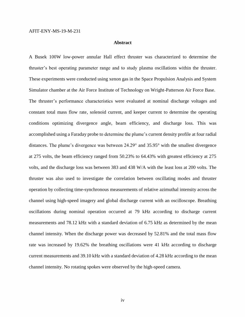
Abstract

A Busek 100W low-power annular Hall effect thruster was characterized to determine the

thruster’s best operating parameter range and to study plasma oscillations within the thruster.

These experiments were conducted using xenon gas in the Space Propulsion Analysis and System

Simulator chamber at the Air Force Institute of Technology on Wright-Patterson Air Force Base.

The thruster’s performance characteristics were evaluated at nominal discharge voltages and

constant total mass flow rate, solenoid current, and keeper current to determine the operating

conditions optimizing divergence angle, beam efficiency, and discharge loss. This was

accomplished using a Faraday probe to determine the plume’s current density profile at four radial

distances. The plume’s divergence was between 24.29° and 35.95° with the smallest divergence

at 275 volts, the beam efficiency ranged from 50.23% to 64.43% with greatest efficiency at 275

volts, and the discharge loss was between 383 and 438 W/A with the least loss at 200 volts. The

thruster was also used to investigate the correlation between oscillating modes and thruster

operation by collecting time-synchronous measurements of relative azimuthal intensity across the

channel using high-speed imagery and global discharge current with an oscilloscope. Breathing

oscillations during nominal operation occurred at 79 kHz according to discharge current

measurements and 78.12 kHz with a standard deviation of 6.75 kHz as determined by the mean

channel intensity. When the discharge power was decreased by 52.81% and the total mass flow

rate was increased by 19.62% the breathing oscillations were 41 kHz according to discharge

current measurements and 39.10 kHz with a standard deviation of 4.28 kHz according to the mean

channel intensity. No rotating spokes were observed by the high-speed camera.


v

Acknowledgments

I would first like to thank my thesis advisor Dr. Hartsfield, a professor at the Air Force

Institute of Technology. Dr. Hartsfield provided invaluable guidance throughout the entire thesis

process, including suggesting what papers to start my background research with, reviewing many

versions of this thesis, and helping assess potential problems and solutions in the lab when things

did not work as expected.

I would also like to thank my other committee members, Major Liu and Dr. Hargus, for

providing their valuable insight and critique.

Additionally, I would like to acknowledge 2d Lt Avery Leonard who took the time to be

in the lab while I was trying to fire the thruster to see how operation was going (or not going) and

for letting me do the same.

I would also like to thank Brian Crabtree at the model shop for manufacturing the

aluminum mounting plate for the cathode.

Lastly, I would like to thank the friends, family, and colleagues who read various versions

of this thesis and provided helpful suggestions to improve its clarity and quality.

Megan N. Maikell

iv

Table of Contents

Page

Abstract .......................................................................................................................................... iv

Acknowledgments .......................................................................................................................... v

Table of Contents ........................................................................................................................... iv

Nomenclature ............................................................................................................................... viii

Tables ............................................................................................................................................ xii

Figures ......................................................................................................................................... xiii

I. Introduction ................................................................................................................................. 1

1.1 Background ............................................................................................................................... 1

1.2 Motivation ................................................................................................................................. 2

1.3 Scope ......................................................................................................................................... 4

1.4 Objectives ................................................................................................................................. 4

II. Background ................................................................................................................................ 7

2.1 Fundamentals of Rocket Propulsion ......................................................................................... 7

2.2 Hall Effect Thruster Fundamentals ......................................................................................... 10

2.2.1 Plume Characteristics........................................................................................................... 11

2.2.2 Anode Characteristics .......................................................................................................... 14

2.2.3 Cathode Characteristics ....................................................................................................... 14

2.2.4 Electron Drift ....................................................................................................................... 17

2.2.5 BHT-100-I-Specific Structure ............................................................................................. 19

2.3 Plasma Fundamentals.............................................................................................................. 21

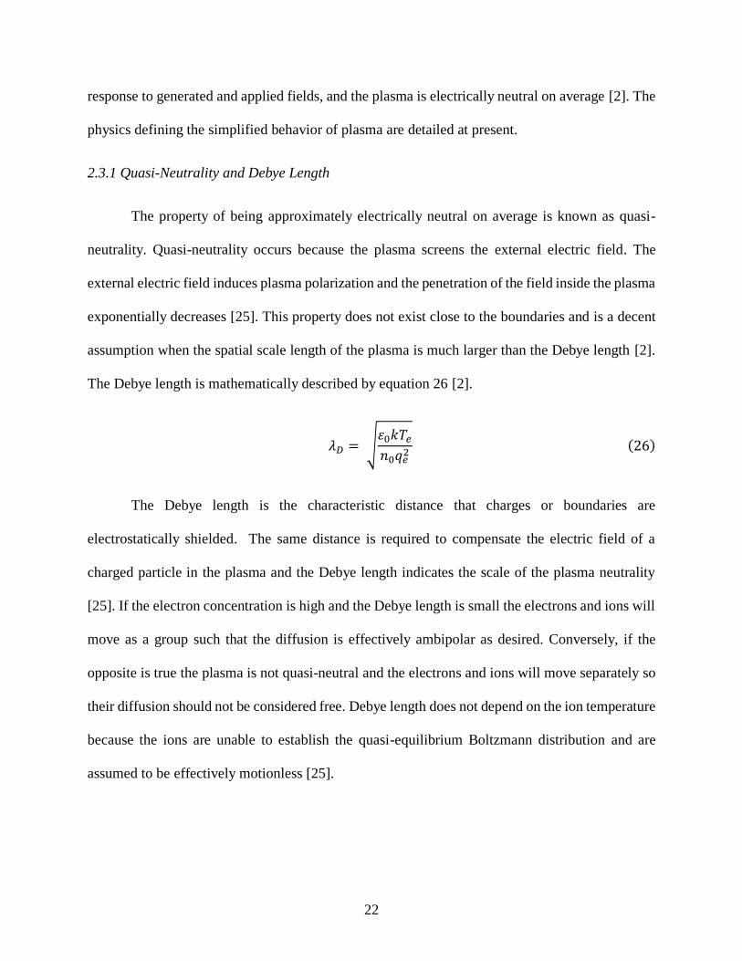
2.3.1 Quasi-Neutrality and Debye Length .................................................................................... 22

2.3.2 Maxwell’s Equations ........................................................................................................... 23

2.3.3 Assumptions ......................................................................................................................... 24

v

Page

2.3.4 Forces and Charged Particle Movement .............................................................................. 24

2.3.5 Classical Diffusion ............................................................................................................... 26

2.3.6 Plasma Oscillations .............................................................................................................. 27

2.4 Plasma Instabilities and Anomalous Diffusion Mechanisms.................................................. 29

2.4.1 Bohm Diffusion ................................................................................................................... 30

2.4.2 Near-Wall Conductivity ....................................................................................................... 30

2.4.3 Rotating Spokes ................................................................................................................... 31

2.5 Faraday Probe ......................................................................................................................... 32

2.6 E × B Probe ............................................................................................................................. 35

2.7 Emissive Probe........................................................................................................................ 38

III. Setup and Methodology .......................................................................................................... 40

3.1 Vacuum Chamber ................................................................................................................... 41

3.1.1 Pumping System .................................................................................................................. 42

3.1.2 Plumbing System ................................................................................................................. 45

3.2 Test Setup................................................................................................................................ 47

3.3 Thruster Operation .................................................................................................................. 51

3.4 Faraday Probe ......................................................................................................................... 53

3.5 E × B Probe ............................................................................................................................. 55

3.6 Emissive Probe........................................................................................................................ 56

3.7 High-Speed Imaging ............................................................................................................... 57

3.8 Oscilloscope ............................................................................................................................ 60

IV. Results and Analysis ............................................................................................................... 62

4.1 Propellant Selection ................................................................................................................ 62

4.2 Power Sources ......................................................................................................................... 63

vi

Page

4.3 Thruster Operation .................................................................................................................. 64

4.4 Effect of Mass Flow Rate on Discharge Current .................................................................... 66

4.5 Thruster Characterization........................................................................................................ 68

4.5.1 Equipment Setbacks ............................................................................................................. 68

4.5.2 Current Density Profile ........................................................................................................ 71

4.5.3 Current Density Profile Calculations ................................................................................... 76

4.5.4 Plume Divergence ................................................................................................................ 79

4.5.5 Maximum Current Density .................................................................................................. 80

4.5.6 Total Beam Current.............................................................................................................. 80

4.5.7 Ion Production Efficiency .................................................................................................... 82

4.6 Anomalous Diffusion .............................................................................................................. 83

4.6.1 Data Synchronization ........................................................................................................... 83

4.6.2 Breathing Mode ................................................................................................................... 85

4.6.3 Spoke Mode ......................................................................................................................... 89

V. Conclusions .............................................................................................................................. 94

5.1 Summary of Results ................................................................................................................ 95

5.2 Next Steps ............................................................................................................................... 96

5.3 Future Work ............................................................................................................................ 96

Appendix A – Thruster Operating Procedures ............................................................................. 99

Preparation .................................................................................................................................... 99

Condition Cathode ........................................................................................................................ 99

Ignite Cathode ............................................................................................................................. 100

Ignite Thruster ............................................................................................................................. 100

Secure Thruster ........................................................................................................................... 101

vii

Page

Appendix B – Characterization Operating Procedures ............................................................... 102

Preparation .................................................................................................................................. 102

Beam Profiler .............................................................................................................................. 103

Appendix C – Anomalous Diffusion Operating Procedures ...................................................... 106

Preparation .................................................................................................................................. 106

High-Speed Camera .................................................................................................................... 107

Emissive Probe............................................................................................................................ 107

Oscilloscope ................................................................................................................................ 110

References ................................................................................................................................... 111

viii

Nomenclature

𝐴 = area (m2)

𝐴𝑎𝑝𝑒𝑟𝑡𝑢𝑟𝑒 = area of the aperture (m2)

𝐴𝑒 = exit area (m2)

𝐵 = magnetic field (T)

𝐵0 = magnetic field normalization constant (T)

𝑐 = speed of light (299792458 m/s)

D = classical cross-field diffusion coefficient (m2/s)

𝐷⊥ = perpendicular classical cross-field diffusion coefficient (m2/s)

𝐷𝐵 = Bohm diffusion coefficient (m2/s)

𝑑 = distance between plates (m)

𝐸 = electric field (V/m)

𝐸𝑝ℎ𝑜𝑡𝑜𝑛 = Energy of a photon (W)

𝑒 = Euler’s number (2.71828)

𝐹 = force (N)

𝐹𝐶 = force due to collisions between particles (N)

𝐹𝐿 = Lorentz force (N)

𝐹𝑃 = pressure gradient force (N)

𝐹𝑡 = divergence correction factor (unitless)

f = frequency (Hz)

𝑓𝑝 = electron angular plasma frequency (rad/s)

𝑔 = gravitational acceleration (9.80665 m/s2)

ℎ = Planck’s constant (6.6261∗ 10−34 m2kg/s)

𝐼𝑏 = beam current (A)

𝐼𝑑 = discharge current (A)

𝐼𝑒,𝑒 = electron emission current (A)

𝐼𝑖 = ion current (A)

𝐼𝑠,𝑐 = electron saturation current (A)

𝐼𝑠,𝑖 = ion saturation current (A)

ix

𝐼𝑠𝑝 = specific impulse (s)

𝐼𝑠𝑝,𝑎 = anode specific impulse (s)

𝐼𝑡 = total impulse (Ns)

𝐽 = current density (A/m2)

𝐽𝑏 = beam current density (A/m2)

𝑘 = Boltzmann’s constant (1.3807 X 10-23 J/K)

𝐿 = characteristic scale length (m)

M = ion mass (kg)

𝑚 = mass (kg)

�̇� = mass flow rate (kg/s)

�̇�𝑎 = anode mass flow rate (kg/s)

𝑚𝑒 = electron mass (9.1094 X 10-31 kg)

𝑚𝑖 = ion mass (kg)

�̇�𝑖 = ion mass flow rate (kg/s)

𝑁 = number of molecules (integer)

𝑛 = particle density (particles/m3)

𝑛𝑒 = electron density (electrons/m3)

𝑛𝑖 = ion density (ions/m3)

𝑛0 = Loschmidt’s number (2.6868 X 1025 m-3)

𝑃 = pressure (Pa)

𝑃𝑏 = beam electrical power (W)

𝑃𝑑 = discharge power (W)

𝑃𝑗𝑒𝑡 = jet power in thruster exhaust (W)

𝑃𝑠𝑦𝑠 = power provided to thruster (W)

𝑝 = momentum (Ns)

𝑞𝑒 = charge of an electron (1.602176487 X 10-19 C)

𝑞𝑖 = charge of an ion (C)

𝑅𝑝𝑙𝑎𝑡𝑒 = resistance of the plate (Ω)

𝑟 = radius, beam radius (m)

𝑟𝐿 = Larmor radius (m)

x

𝑇 = thrust (N), temperature (K)

𝑇𝑒 = electron temperature (K)

𝑡 = time (s)

𝑡𝑓 = final time (s)

𝑡0 = initial time (s)

𝑉𝑏 = net beam voltage (V)

𝑉𝑑 = discharge voltage (V)

𝑉𝑑𝑟𝑜𝑝 = voltage drop (V)

𝑉𝑓 = emissive probe floating potential (V)

𝑉𝑖 = ionization potential (V)

𝑉𝑝 = plasma potential (V)

𝑣 = velocity (m/s)

𝑣⊥ = perpendicular component of velocity (m/s)

𝑣𝑎 = velocity of particle a (m/s)

𝑣𝑏 = velocity of particle b (m/s)

𝑣𝑐 = critical velocity (m/s)

𝑣𝐷 = diamagnetic drift velocity (m/s)

𝑣𝑑 = electron drift velocity (m/s)

𝑣𝐸 = azimuthal 𝑬 × 𝑩 drift velocity (m/s)

𝑣𝑒 = exhaust velocity (m/s)

𝑣𝑒,𝑎 = anode effective exit velocity (m/s)

𝑣𝑖 = ion velocity (m/s)

𝑣𝑡ℎ = thermal drift velocity (m/s)

z = charge state of the ion (integer)

𝛼 = multiply charged ions correction factor (unitless)

𝛼𝐿,𝑅 = Faraday probe correction factor angles (rad)

Γ𝑒 = cross field electron flux (Vm)

Δ𝑉𝑖 = accelerating voltage of ion (V)

∆𝑣 = change in velocity (m/s)

∆𝜙 = voltage difference between the plates (V)

xi

𝜀0 = permittivity of free space (8.8542 X 10-12 A2s4/m3kg)

𝜁𝑖 = ion species fraction (unitless)

𝜂 = total thruster efficiency (unitless)

𝜂𝑎 = anode efficiency (unitless)

𝜂𝑐 = cathode efficiency (unitless)

𝜂𝑚𝑎𝑔 = electromagnetic coil efficiency (unitless)

𝜂𝑠𝑦𝑠 = power system efficiency (unitless)

𝜃 = angle, average half- angle divergence of the beam (rad)

𝜅𝐴 = Faraday probe area correction factor (unitless)

𝜅𝐷 = Faraday probe distance correction factor (unitless)

𝜆 = wavelength (m)

𝜆𝐷 = Debye length (m)

𝜇 = electron mobility (m2/Vs)

𝜇⊥ = perpendicular electron mobility (m2/Vs)

𝜇0 = permeability of free space (1.25664 X 10-6 m kg/s2 A2)

𝜐 = collision frequency (Hz)

𝜐𝑎𝑏 = collision frequency between particles a and b (Hz)

𝜌 = charge density (C/m3)

𝜏 = average collision time (Hz)

Ωe = electron Hall parameter (unitless)

Ω𝑖 = beam current fraction (unitless)

Ω𝑝 = ion plasma frequency (Hz)

𝜔𝑐 = electron gyrofrequency (Hz)

𝜔𝑝 = electron plasma frequency (Hz)

xii

Tables

Page

Table 1. Typical Operating Parameters for Thrusters ....................................................................10

Table 2. Plasma Oscillation Regions .............................................................................................28

Table 3. Performance Test Data Comparison ................................................................................65

Table 4. Current Density Profile Calculations ...............................................................................77

Table 5. Breathing Mode Operating Parameters............................................................................85

Table 6. Spoke Mode Operating Parameters .................................................................................89

xiii

Figures

Page

Figure 1. HET Cross-Sectional Schematic of Basic Operating Principles ....................................11

Figure 2. Hollow Cathode Schematic ............................................................................................15

Figure 3. HET Azimuthal Drift Depiction .....................................................................................17

Figure 4. Downstream View of BHT-100-I with BHC-1500 ........................................................20

Figure 5. BHT-100-I and BHC-1500 Electrical Diagram .............................................................21

Figure 6. Faraday Probe Geometry to Thruster .............................................................................33

Figure 7. Electric and Magnetic Fields within E × B Probe ..........................................................36

Figure 8. SPASS Vacuum Chamber ..............................................................................................42

Figure 9. Screwline 250 Pump .......................................................................................................43

Figure 10. CVI TM150 (top) and CVI TM500 (side) ....................................................................43

Figure 11. CBST 6.0 Compressors ................................................................................................44

Figure 12. Residual Gas Analyzer Vacuum Plus User Interface ...................................................45

Figure 13. Propellant Line Plumbing .............................................................................................46

Figure 14. MKS Type 247 4 Channel Readout..............................................................................46

Figure 15 Test Setup Diagram .......................................................................................................47

Figure 16. Test Setup Inside Chamber for Phase One ...................................................................48

Figure 17. Labview User Interface for Phase One .........................................................................49

Figure 18. Test Setup Inside Chamber for Phase Two ..................................................................50

Figure 19. Labview User Interface for Phase Two ........................................................................51

Figure 20. Banana Plug and BNC Electrical Connections Rack ...................................................52

Figure 21. Faraday Probe ...............................................................................................................53

Figure 22. Faraday Probe Schematic .............................................................................................54

Figure 23. E × B Probe ..................................................................................................................55

Figure 24. Emissive Probe .............................................................................................................56

Figure 25. Emissive Probe Circuit .................................................................................................57

Figure 26. Shimadzu Hyper Vision HPV-2 Camera ......................................................................58

Figure 27. Simplified Image Analysis of HET Channel ................................................................59

Figure 28. Simplified Data Image Examples for Analysis ............................................................59

xiv

Page

Figure 29. Example of Emissive Probe Occlusion ........................................................................60

Figure 30. BHT-100-I with Krypton Gas ......................................................................................63

Figure 31. BHT-100-I with Xenon Gas .........................................................................................63

Figure 32. Discharge Voltage v. Current for Different Total Mass Flow Rates ............................67

Figure 33. Discharge Voltage v. Power for Different Total Mass Flow Rates ..............................67

Figure 34. Water Leak from Traverse Cooling System Inside Chamber ......................................69

Figure 35. RGA Output during HET Operation ............................................................................70

Figure 36. RGA Output during HET and Traverse Operation.......................................................70

Figure 37. Faraday Probe Current Density Measurements at 200V ..............................................72

Figure 38. Normalized Faraday Probe Current Density Measurements at 200V ..........................72







Figure 45. Divergence as a Function of Discharge Voltage ..........................................................79

Figure 46. Maximum Current Density as a Function of Discharge Voltage .................................80

Figure 47. Beam Current as a Function of Discharge Voltage ......................................................80

Figure 48. Total Beam Current as a Function of Radial Distance .................................................81

Figure 49. Ion Production Efficiency as a Function of Discharge Current ...................................82

Figure 50. BHT-100-I Jet Plume During Operation ......................................................................83

Figure 51. High-Speed Camera Live Video Feed ..........................................................................84

Figure 52. Breathing Mode Projected Channel Plot with Arbitrary Intensity ...............................85

Figure 53. Breathing Mode Channel Plot with Arbitrary Intensity and Min Cutoff Intensity ......86

Figure 54. Breathing Mode Discharge Current ..............................................................................86

Figure 55. Breathing Mode Projected Channel Plot with Arbitrary Intensity ...............................87

Figure 56. Breathing Mode Discharge Current ..............................................................................87

Figure 57. Breathing Mode Breathing Oscillations .......................................................................88

Figure 58. Breathing Mode Breathing Oscillation Frequency Histogram .....................................89

xv

Page

Figure 59. Spoke Mode Projected Channel Plot with Arbitrary Intensity and Min Cutoff ...........90

Figure 60. Spoke Mode Projected Channel Plot with Arbitrary Intensity and Min Cutoff ...........91

Figure 61. Spoke Mode Discharge Current ...................................................................................91

Figure 62. Spoke Mode Breathing Oscillations .............................................................................92

Figure 63. Spoke Mode Breathing Oscillation Frequency Histogram ...........................................93

Figure 64. Beam Mapper Overview Diagram ..............................................................................102

Figure 65. AFITPROGRAM.vi Main Page User Interface .........................................................103

Figure 66. Radial Scans User Interface........................................................................................104

Figure 67. Linear Scans Emissive User Interface ........................................................................106

Figure 68. Emissive Probe Generate Digital User Interface ........................................................108

Figure 69. Emissive Probe and PicoScope User Interface ...........................................................109

1

CHARACTERIZATION AND ANOMALOUS



I. Introduction

1.1 Background

Hall effect thrusters (HETs) have emerged as a leading electric propulsion technology in

terms of thrust, specific impulse, and efficiency. Electric propulsion relies on the acceleration of

gases for propulsion by electrical heating or by the combination of electric and magnetic forces.

HETs fall within the electrostatic propulsion subdivision of electric propulsion [1]. These thrusters

generally operate in power ranges of hundreds of Watts to tens of kilowatts with a specific impulse

anywhere from several hundred seconds to thousands of seconds [2]. The specific impulse of

HETs is significantly greater than those of chemical propulsion systems and HETs. Additionally,

HETs typically have thrust levels on the scale of a fraction of a Newton (depending on discharge

power), making them an ideal option for station keeping. This is because only small amounts of

thrust are required for station keeping and propellant mass is minimized.

HETs are most commonly used for station keeping because of their specific impulse and

thrust capabilities. However, HETs are not limited to station keeping; it simply takes HETs longer

than chemical propulsion systems to provide the change in velocity needed for orbit transfers.

HETs have been used for large orbit transfers by design [3] and as a solution to primary propulsion

system failure [4]. HETs have also been to decrease the altitude of the satellite’s orbit after mission

completion [5]. The purpose of this is to accelerate the orbital decay and thereby decrease the

2

amount of time before the satellite reenters the atmosphere. Additionally, HETs are considered

viable options for deep space missions [6] and formation flying [7].

The first working HETs were reported independently in America and Russia in the 1960s.

In December of 1971 the Soviets successfully operated the first pair of HETs in space aboard the

Meteor weather satellite [8]. The two thrusters, SPT-60s, were operational for more than 170 hours

and raised the satellite’s orbit altitude by 17 kilometers into a sun-synchronous orbit [9]. Since

their initial on-orbit success in 1971, HETs have gained considerable flight heritage and global

popularity within government-sponsored and commercial led space programs. Over 140 HETs

have operated in space since the first on-orbit test in 1971 [2] and the use of electric propulsion on

spacecraft continues to grow globally as reliability, flight heritage, and cost benefits increase.

1.2 Motivation

A primary advantage of electric propulsion over chemical propulsion systems is its power

source. Power required for HET operation is provided directly by the spacecraft’s power

subsystem as compared to the fixed amount of internal energy of the propellant [8]. This means

the amount of power supplied to the HET is limited by the technology available and size of the

solar arrays. This amount of power is expected to increase as advancements to power subsystem

components are made. These advances can decrease the amount of propellant mass needed,

reducing the overall mass of the satellite and the concurrent cost of the launch. Electric propulsion

systems are also more precise with their thrust level adjustability compared to chemical systems,

have a shutdown and restart capability, long lifetime, and can use chemically passive propellants

safer to handle than most of the propellants used in chemical systems [10]. Compared to other

forms of electric propulsion, HETs typically have higher specific power and higher thrust to power

3

ratios [8]. HETs also generally have less mass and are physically smaller than other forms of

electric propulsion [8].

Although HETs are already favored for their ability to reduce spacecraft mass, efforts are

being made to further increase their advantage over other propulsion systems by improving their

performance. These efforts include lowering the beam divergence angle, reducing and

characterizing electromagnetic interference with the spacecraft, decreasing erosion rates and

thereby increasing HET lifetime, raising the thrust to power ratio as much as physically possible,

increasing thrust efficiency, and scaling the power [11, 12] from tens of Watts up to 100 kilowatts

[8]. HETs are designed with greater capabilities due to the rapid rise in spacecraft power able to

support such subsystems as well as for spacecraft missions requiring propulsion systems with

greater efficiency, lifetime, and operating envelopes [8]. Understanding the dynamics within the

thruster channel and plume is essential to make these improvements in a time and cost-saving

manner.

Although HETs have been studied and characterized since the 1960s, the plasma dynamics

within the channel and plume remain an active area of research because they are not fully

understood [12, 13, 14]. Internal plasma measurements demonstrate classical diffusion theory

based on collision frequency cannot be the only transport mechanism enhancing cross-field

mobility [8, 15]. This has led to non-classical, or anomalous diffusion theory, and is thought to be

caused by a combination of several different mechanisms. The two most commonly proposed

anomalous transport mechanisms are Bohm diffusion and near-wall conductivity. An observed

effect of an unknown, additional mechanism causing transport across the magnetic field is referred

to as the rotating spoke. A connection between increased cathode electron emission and reduced

transport has been observed [3], however, better understanding of the spokes are required to

4

determine what mechanism causes the additional transport, or rather, what the causal relationship

between plasma instabilities and anomalous diffusion modes is. This is an important phenomenon

to understand and reduce because anomalous diffusion causes excessive cross-field current and

shifts the ion accelerating region outside of the thruster channel. This shift results in a more

diverged plasma plume and diminishes HET efficiency because it limits the maximum achievable

electric field [16].

1.3 Scope

The focus of this research is the characterization of the Busek 100 Watt long-life, low

power annular HET (BHT-100-I) and the observation of plasma oscillations within the thruster.

Data from the HET’s nominal operating boundaries is used to characterize the thruster using a

Faraday probe and E × B probe to determine the plume divergence angle, current density profile,

and ion species fractions at these operating modes. Plasma instability is induced by decreasing the

discharge voltage and increasing propellant flow to the thruster to observe the rotating spokes

phenomenon associated with anomalous diffusion. During this operating mode, concurrent

measurements of the local plasma potential are measured with an emissive probe, visible emissions

are captured using a high-speed camera capable of collecting data at one million frames per second,

and discharge current is measured with an oscilloscope.

1.4 Objectives

Hall thrusters are a viable propulsion alternative for station keeping, collision avoidance,

orbit transfers, formation flying, and deep space missions. This research is being conducted

because the BHT-100-I and HET plasma dynamics are not fully understood. The BHT-100-I

features several modifications intended to increase the lifetime of the thruster, but this, as well as

5

any secondary effects of these modifications, is experimentally untested. The BHT-100-I’s

performance has only been established for pre-delivery check-out purposes by Busek.

Experimental testing is performed at facilities located at the Air Force Institute of Technology

(AFIT) on Wright-Patterson Air Force Base. Specifically, the Space Propulsion Analysis and

System Simulator (SPASS) chamber. Experiments use pressurized xenon gas as the propellant.

The objectives of this research are as follows:

a. Verify the BHT-100-I operates as expected by comparing experimental results to

performance test data from pre-delivery check-out provided by Busek.

b. Vary the discharge voltage to develop performance curves for current density, divergence

angle, ion species, and efficiency at several nominal operating conditions by conducting

radial sweeps with a Faraday probe and E × B probe at 20, 30, 40, and 50 centimeters from

the thruster face in one degree increments with a five second dwell time per angle.

c. Determine the optimal range of operating conditions (by varying discharge voltage)

yielding greatest efficiency, smallest divergence angle, and highest single ionization

fraction.

d. Correlate non-intrusive visual measurements of plasma emission with a high-speed

camera, discharge current with a non-intrusive oscilloscope, and plasma potential with an

intrusive emissive probe at nominal conditions (breathing mode).

e. Correlate non-intrusive visual measurements of plasma emission with a high-speed

camera, discharge current with a non-intrusive oscilloscope, and plasma potential with an

intrusive emissive probe at non-optimal conditions (spoke mode).

Apart from gaining a better understanding of the operation of the BHT-100-I, the results of

this research may be used to aid in future HET development. The results could also be used to

6

improve or confirm existing numerical models and simulations, help develop future thruster

designs, and improve comparisons between vacuum chamber experiments and on-orbit plume

simulations.

7

II. Background

2.1 Fundamentals of Rocket Propulsion

All rocket propulsion systems are based on Newton’s second law of motion that states the

sum of the forces acting on the system are equal to the time rate of change of momentum of the

system. Assuming the velocity and mass are functions of time where mass is expelled at a constant

rate and constant exhaust velocity opposite to its direction of motion, the sum of the forces acting

on the body for a closed system is modeled by equation 1 [17].

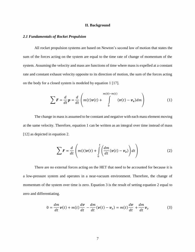
∑ 𝑭 =𝑑

𝑑𝑡𝒑 =

𝑑

𝑑𝑡 (𝑚(𝑡)𝒗(𝑡) + ∫ (𝒗(𝑡) − 𝒗𝒆)𝑑𝑚

𝑚(0)−𝑚(𝑡)

0

) (1)

The change in mass is assumed to be constant and negative with each mass element moving

at the same velocity. Therefore, equation 1 can be written as an integral over time instead of mass

[12] as depicted in equation 2.

∑ 𝑭 =𝑑

𝑑𝑡 (𝑚(𝑡)𝒗(𝑡) + ∫ (

𝑑𝑚

𝑑𝑡(𝒗(𝑡) − 𝒗𝒆)) 𝑑𝑡

𝑡

0

) (2)

There are no external forces acting on the HET that need to be accounted for because it is

a low-pressure system and operates in a near-vacuum environment. Therefore, the change of

momentum of the system over time is zero. Equation 3 is the result of setting equation 2 equal to

zero and differentiating.

0 =𝑑𝑚

𝑑𝑡𝒗(𝑡) + 𝑚(𝑡)

𝑑𝒗

𝑑𝑡 −

𝑑𝑚

𝑑𝑡(𝒗(𝑡) − 𝒗𝑒) = 𝑚(𝑡)

𝑑𝒗

𝑑𝑡 +

𝑑𝑚

𝑑𝑡𝒗𝑒 (3)

8

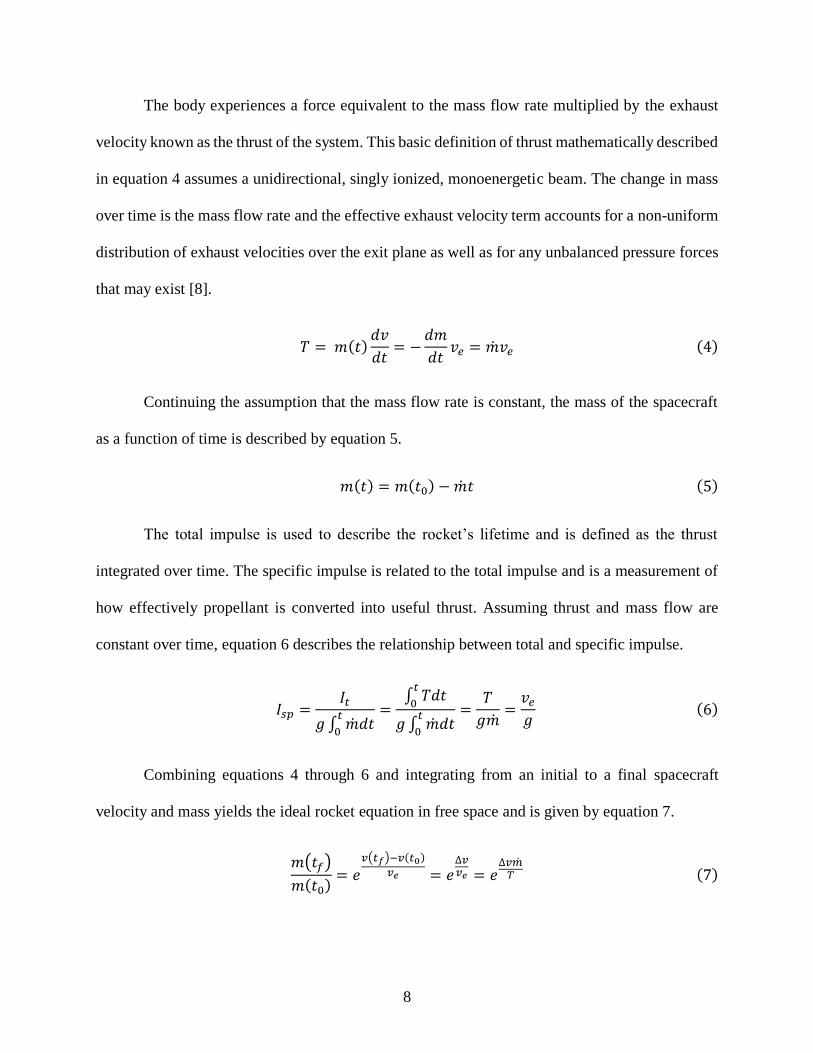
The body experiences a force equivalent to the mass flow rate multiplied by the exhaust

velocity known as the thrust of the system. This basic definition of thrust mathematically described

in equation 4 assumes a unidirectional, singly ionized, monoenergetic beam. The change in mass

over time is the mass flow rate and the effective exhaust velocity term accounts for a non-uniform

distribution of exhaust velocities over the exit plane as well as for any unbalanced pressure forces

that may exist [8].

𝑇 = 𝑚(𝑡)𝑑𝑣

𝑑𝑡= −

𝑑𝑚

𝑑𝑡𝑣𝑒 = �̇�𝑣𝑒 (4)

Continuing the assumption that the mass flow rate is constant, the mass of the spacecraft

as a function of time is described by equation 5.

𝑚(𝑡) = 𝑚(𝑡0) − �̇�𝑡 (5)

The total impulse is used to describe the rocket’s lifetime and is defined as the thrust

integrated over time. The specific impulse is related to the total impulse and is a measurement of

how effectively propellant is converted into useful thrust. Assuming thrust and mass flow are

constant over time, equation 6 describes the relationship between total and specific impulse.

𝐼𝑠𝑝 =𝐼𝑡

𝑔 ∫ �̇�𝑑𝑡𝑡

0

=∫ 𝑇𝑑𝑡

𝑡

0

𝑔 ∫ �̇�𝑑𝑡𝑡

0

=𝑇

𝑔�̇�=

𝑣𝑒

𝑔(6)

Combining equations 4 through 6 and integrating from an initial to a final spacecraft

velocity and mass yields the ideal rocket equation in free space and is given by equation 7.

𝑚(𝑡𝑓)

𝑚(𝑡0)= 𝑒

𝑣(𝑡𝑓)−𝑣(𝑡0)

𝑣𝑒 = 𝑒∆𝑣𝑣𝑒 = 𝑒

∆𝑣�̇�𝑇 (7)

9

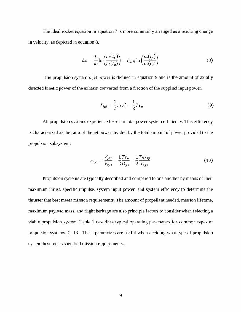
The ideal rocket equation in equation 7 is more commonly arranged as a resulting change

in velocity, as depicted in equation 8.

∆𝑣 =𝑇

�̇�ln (

𝑚(𝑡𝑓)

𝑚(𝑡0)) = 𝐼𝑠𝑝𝑔 ln (

𝑚(𝑡𝑓)

𝑚(𝑡0)) (8)

The propulsion system’s jet power is defined in equation 9 and is the amount of axially

directed kinetic power of the exhaust converted from a fraction of the supplied input power.

𝑃𝑗𝑒𝑡 =1

2�̇�𝑣𝑒

2 =1

2𝑇𝑣𝑒 (9)

All propulsion systems experience losses in total power system efficiency. This efficiency

is characterized as the ratio of the jet power divided by the total amount of power provided to the

propulsion subsystem.

𝜂𝑠𝑦𝑠 =𝑃𝑗𝑒𝑡

𝑃𝑠𝑦𝑠=

1

2

𝑇𝑣𝑒

𝑃𝑠𝑦𝑠=

1

2

𝑇𝑔𝐼𝑠𝑝

𝑃𝑠𝑦𝑠

(10)

Propulsion systems are typically described and compared to one another by means of their

maximum thrust, specific impulse, system input power, and system efficiency to determine the

thruster that best meets mission requirements. The amount of propellant needed, mission lifetime,

maximum payload mass, and flight heritage are also principle factors to consider when selecting a

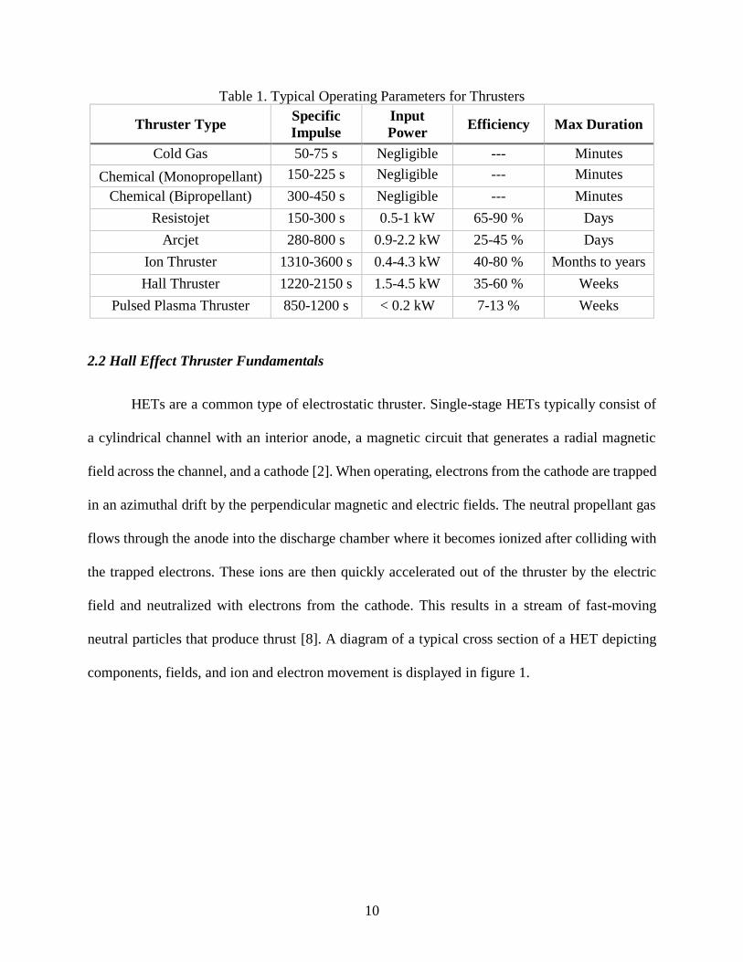
viable propulsion system. Table 1 describes typical operating parameters for common types of

propulsion systems [2, 18]. These parameters are useful when deciding what type of propulsion

system best meets specified mission requirements.

10

Table 1. Typical Operating Parameters for Thrusters

Thruster Type Specific

Impulse

Input

Power Efficiency Max Duration

Cold Gas 50-75 s Negligible --- Minutes

Chemical (Monopropellant) 150-225 s Negligible --- Minutes

Chemical (Bipropellant) 300-450 s Negligible --- Minutes

Resistojet 150-300 s 0.5-1 kW 65-90 % Days

Arcjet 280-800 s 0.9-2.2 kW 25-45 % Days

Ion Thruster 1310-3600 s 0.4-4.3 kW 40-80 % Months to years

Hall Thruster 1220-2150 s 1.5-4.5 kW 35-60 % Weeks

Pulsed Plasma Thruster 850-1200 s < 0.2 kW 7-13 % Weeks

2.2 Hall Effect Thruster Fundamentals

HETs are a common type of electrostatic thruster. Single-stage HETs typically consist of

a cylindrical channel with an interior anode, a magnetic circuit that generates a radial magnetic

field across the channel, and a cathode [2]. When operating, electrons from the cathode are trapped

in an azimuthal drift by the perpendicular magnetic and electric fields. The neutral propellant gas

flows through the anode into the discharge chamber where it becomes ionized after colliding with

the trapped electrons. These ions are then quickly accelerated out of the thruster by the electric

field and neutralized with electrons from the cathode. This results in a stream of fast-moving

neutral particles that produce thrust [8]. A diagram of a typical cross section of a HET depicting

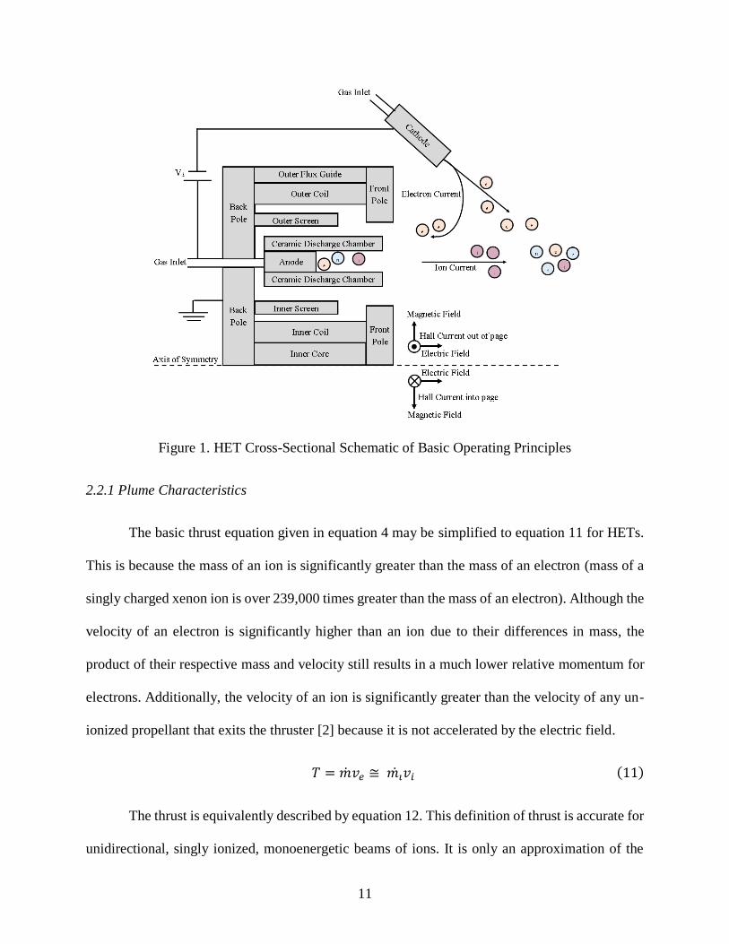
components, fields, and ion and electron movement is displayed in figure 1.

11

Figure 1. HET Cross-Sectional Schematic of Basic Operating Principles

2.2.1 Plume Characteristics

The basic thrust equation given in equation 4 may be simplified to equation 11 for HETs.

This is because the mass of an ion is significantly greater than the mass of an electron (mass of a

singly charged xenon ion is over 239,000 times greater than the mass of an electron). Although the

velocity of an electron is significantly higher than an ion due to their differences in mass, the

product of their respective mass and velocity still results in a much lower relative momentum for

electrons. Additionally, the velocity of an ion is significantly greater than the velocity of any un-

ionized propellant that exits the thruster [2] because it is not accelerated by the electric field.

𝑇 = �̇�𝑣𝑒 ≅ 𝑚𝑖̇ 𝑣𝑖 (11)

The thrust is equivalently described by equation 12. This definition of thrust is accurate for

unidirectional, singly ionized, monoenergetic beams of ions. It is only an approximation of the

12

thrust produced by a HET because it does not account for the divergence of the ion beam or the

presence of multiply charged ions.

𝑇 = (𝐼𝑏𝑀

𝑞𝑒) (√

2𝑞𝑒𝑉𝑏

𝑀) = 𝐼𝑏√

2𝑀𝑉𝑏

𝑞𝑒

(12)

Loss of momentum associated with the plume’s divergence can be calculated when the

input mass flow, measured thrust, and mass-weighted average velocity are known. There is no

consistent method for calculating the effect of plume momentum divergence on thrust because

measuring particle velocity throughout the plume is difficult [19]. One method for approximating

the plume momentum divergence for cylindrical HETs is by using the charge-weighted

divergence. The primary difference between the two results originates from spatial variation of the

average ion charge and mass utilization in the plume [19]. Using the divergence approximation,

the thrust correction factor for a cylindrical HET is mathematically described by equation 13 [2].

𝐹𝑡 =∫ 2𝜋𝑟𝐽(𝑟) cos 𝜃(𝑟)𝑑𝑟

𝑟

0

𝐼𝑏

(13)

The ion current density and half-angle divergence of the beam are functions of the beam

radius. If the ion current density is assumed to be constant as a function of radius the thrust

correction factor for beam divergence is further simplified to the cosine of the average half-angle

divergence of the beam.

In order to account for the effect of multiply charged ion species on the thrust produced by

the HET, an additional correction factor is required [2]. This correction factor is mathematically

expressed by equation 14, where the counter represents the charged state of the ion.

13

𝛼 =

∑1

√𝑖 𝐼𝑖 𝑖=1

∑ 𝐼𝑖 𝑖=1 (14)

Ions can become multiply charged as the result of multiple collisions or as the result of a

single collision with enough kinetic energy to reach a higher ionization state. Although multiply

charged ions are regularly observed in HET plumes, the amount of each species present in the

plume is expected to decrease with each increase in ionization state. This is because the amount of

energy required for ionization increases with each ionization state (roughly 12, 21, 32, 46 and 57

eV for xenon [20]) and the ion accelerates out of the HET as soon as it is ionized. The rapid

acceleration of the ion significantly decreases the probability of a second collision in the channel

because its time in the channel after ionization is so brief.

Collisions occur in the plume as well. Some of these collisions are required for plume

neutralization (between ions and electrons), but others are collisions between two ions or between

ions and neutral particles. These collisions result in charge exchange. Charge exchange occurs in

vacuum chamber testing more than on orbit due to background pressure in the chamber and the

exchange is greatest at the wings of the plume [21]. Additional collisions in the wings occur in

vacuum chamber tests because of the plume’s close proximity to the walls of the chamber.

Using the two correction factors expressed in equations 13 and 14 as well as the

relationship in equation 12, the thrust of a HET is best described by equation 15. The divergence

of the plume and the presence of multiply charged ions decrease the amount of thrust produced.

𝑇 = 𝐹𝑡 𝛼 𝐼𝑏√2𝑀𝑉𝑏

𝑞𝑒

(15)

14

The amount of power resulting from the beam of accelerated ions is described by equation

16 and is always less than the amount of discharge power applied to the system. This is because

of various loss mechanisms including thermal radiation, collisions with the channel walls, and

electron collection at the anode [12].

𝑃𝑏 = 𝐼𝑏𝑉𝑏 = 𝑛𝑖𝑞𝑖𝑣𝑖𝐴𝑒𝑉𝑏 < 𝑃𝑑 (16)

2.2.2 Anode Characteristics

When operated, the HET’s anode acts as the positive electrode for the applied voltage and

distributes the propellant gas uniformly into the chamber. This is usually done with a series of

equally spaced injection ports around the circumference of the anode, although some HETs have

separate anode and gas injector components [8]. The anode’s performance is defined by its

efficiency, discharge power, anode specific impulse, and thrust.

𝑣𝑒,𝑎 =𝑣𝑒

𝜂𝑐=

𝑇

�̇�𝑎

(17)

𝐼𝑠𝑝,𝑎 =𝐼𝑠𝑝

𝜂𝑐=

𝑇

�̇�𝑎𝑔 (18)

𝜂𝑎 =𝜂

𝜂𝑐𝜂𝑚𝑎𝑔=

𝑇2

2�̇�𝑎𝑃𝑑=

𝑇2

2�̇�𝑎𝐼𝑑𝑉𝑑 (19)

These parameters characterize how thruster operation is affected by voltage and mass flow

rate changes and are used to assess how various operating points affect thruster processes [8].

2.2.3 Cathode Characteristics

The cathode is responsible for supplying electrons to the chamber to ionize the propellant

and into the plasma plume to neutralize the accelerating ions [8] in order to maintain a spacecraft

15

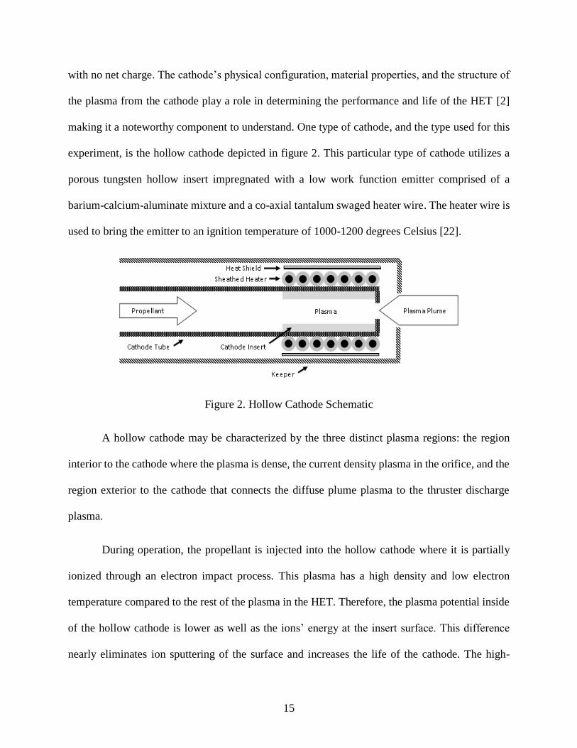
with no net charge. The cathode’s physical configuration, material properties, and the structure of

the plasma from the cathode play a role in determining the performance and life of the HET [2]

making it a noteworthy component to understand. One type of cathode, and the type used for this

experiment, is the hollow cathode depicted in figure 2. This particular type of cathode utilizes a

porous tungsten hollow insert impregnated with a low work function emitter comprised of a

barium-calcium-aluminate mixture and a co-axial tantalum swaged heater wire. The heater wire is

used to bring the emitter to an ignition temperature of 1000-1200 degrees Celsius [22].

Figure 2. Hollow Cathode Schematic

A hollow cathode may be characterized by the three distinct plasma regions: the region

interior to the cathode where the plasma is dense, the current density plasma in the orifice, and the

region exterior to the cathode that connects the diffuse plume plasma to the thruster discharge

plasma.

During operation, the propellant is injected into the hollow cathode where it is partially

ionized through an electron impact process. This plasma has a high density and low electron

temperature compared to the rest of the plasma in the HET. Therefore, the plasma potential inside

of the hollow cathode is lower as well as the ions’ energy at the insert surface. This difference

nearly eliminates ion sputtering of the surface and increases the life of the cathode. The high-

16

density plasma in the insert region also eliminates space charge effects that could limit electron

emission current density at the cathode surface [2].

An orifice at the end of the emitter tube restricts the downstream gas flow and establishes

a pressure within the cathode emitter tube. The current density is highest at the orifice for this

reason. There must be sufficient plasma density generated in this region to carry the current. The

discharge current flowing through the orifice is described by equation 20.

𝐼𝑑 = 𝑛𝑒𝑞𝑒𝑣𝑑𝐴 (20)

The electron drift velocity in equation 20 must be significantly smaller than the thermal

drift velocity. This relationship is determined by the plasma electron temperature at the emitter

orifice and is mathematically described by equation 21 [2].

𝑣𝑑 =𝐼𝑑

𝑛𝑒𝑞𝑒𝐴 ≪ √

𝑘𝑇𝑒

𝑚𝑒 = 𝑣𝑡ℎ (21)

The plume region begins where the plasma and ionized neutral gas start to expand. This

plasma and expanding ionized gas are used to neutralize the accelerated ions from the HET channel

and to ionize the neutral propellant coming from the anode (reference figure 1).

The life of the keeper has strong effects on the life of the cathode and thruster [2], making

it a vital component to understand. The keeper is an electrode that encases the entire cathode and

serves several functions that benefit cathode operation. The keeper facilitates turning on the

cathode discharge, sustains an internal discharge before establishing thruster operation, maintains

cathode operation and temperature if the discharge or beam current is briefly interrupted, and

protects the orifice plate and external heater from ion bombardment that would otherwise limit the

17

cathode’s life. Furthermore, the keeper is typically biased positive in relation to the cathode to

initiate the discharge during start-up and reduce ion bombardment energy during operation [2].

2.2.4 Electron Drift

The electrons that enter the chamber from the cathode are subject to an azimuthal drift

around the radial magnetic field lines as a result of the perpendicular magnetic and axial electric

fields. This electron drift velocity is depicted in figure 3 (and figure 1) and is given by equation 22

[1].

𝒗𝐸 = 𝑬 × 𝑩

𝐵02 (22)

Figure 3. HET Azimuthal Drift Depiction

The electrons are trapped in this closed drift due to the strength of the magnetic field,

increasing the electron residence time in the channel so the electrons and neutral particles injected

through the anode collide inelastically to ionize the propellant [1, 8]. Ionization results from these

electron-neutral collisions when the kinetic energy of the electron is greater than the first ionization

energy of the neutral gas. This sets a minimum electron drift velocity, or critical velocity, that is

18

mathematically expressed by equation 23 [2] using the law of the conservation of energy. Equation

23 assumes the electron correction term may be neglected because 𝑞𝑒𝑉𝑖 ≫1

2𝑚𝑒𝑣𝑒

2 in HETs.

1

2𝑚𝑒𝑣𝑐

2 = 𝑞𝑒𝑉𝑖 +1

2𝑚𝑒𝑣𝑒

2 ≅ 𝑞𝑒𝑉𝑖 (23)

The electrons are also required to be magnetized for proper HET operation, meaning the

electrons must make many orbits around a magnetic field line between collisions with a neutral or

ion that result in cross-field diffusion [2]. The electrons are considered magnetized when the

characteristic length scale is significantly larger than the electron Larmor radius as stated in

equation 24. The characteristic length scale is the length of the portion of the discharge chamber

where the electric field is positive and large and is approximately the length of the acceleration

region [8]. The Larmor radius is the radius of the particle’s circular gyration opposite to the

induced magnetic field.

𝑟𝐿 =𝑚𝑒𝑣⊥

𝑞𝑒𝐵=

𝑚𝑒𝐸

𝑞𝑒𝐵2≪ 𝐿 (24)

The magnetic field is not strong enough to trap the ions in an azimuthal drift within the

channel due to their significantly larger mass (on the order of 105 times greater). This increase in

mass means the ions have a significantly larger Larmor radius than the trapped electrons. The ions

are accelerated by the axial electric field out of the channel because their Larmor radius is much

greater than the channel characteristic length [2, 8, 11]. As this acceleration occurs, an axial

electron flux equivalent to the ion flux reaches the anode. This is due to cross-field mobility and

this same flux of electrons is provided by the cathode to neutralize the exhausted ions. This allows

quasi-neutrality to be maintained and ensures there is no space-charge limit imposed on the

acceleration [11].

19

The electrons must experience an adequate number of collisions on their route to the anode

and maintain an azimuthal current several times larger than the axial current to sustain the plasma

discharge [8]. This occurs when the square of the Hall parameter, a function of electron

gyrofrequency and collision frequency (reference equation 34), is significantly larger than unity

[2, 8]. This relationship is mathematically depicted by equation 25.

Ω𝑒2 = (

𝜔𝑐

𝜐)

2

= (𝑞𝑒𝐵

𝑚𝑒𝜈)

2

≫ 1 (25)

There is not enough energy to ionize the neutral propellant if the magnetic field is too

strong (equation 22 and 23) and the electrons will not be magnetized (needed for sustained

ionization) if the magnetic field is too weak (equation 24 and 25). It is therefore reasonable to

assume that efficient HET operation exists over a limited range of operating parameters and that

there will always be an optimum magnetic field strength to maximize thruster efficiency.

2.2.5 BHT-100-I-Specific Structure

The BHT-100-I has the basic structure shown in figure 1 but features an additional

permanent magnet under the nose cone and boron nitride lining at the exit plane. Both

modifications intend to decrease erosion and thus increase the lifetime of the thruster. The plasma

is generated at the end of the annular discharge channel and the magnetic circuit is driven by an

electromagnet. There are also plasma ground screens to shield the high voltage anode surfaces

from the plasma on the internal portion of the thruster. This was also done to increase the thruster’s

lifetime. Additionally, this specific model uses materials and coatings that are iodine compatible

[23] although the BHT-100-I was designed to use xenon as the propellant.

20

Iodine has been found to have similar performance to xenon with the BHT-200 except at

high discharge voltages where iodine was superior [24]. Iodine is easier to ionize than xenon (lower

ionization potential) but it is also solid at room temperature and electronegative with the ability to

oxidize certain materials [24], leading to a complex propellant supply system and additional

durability issues.

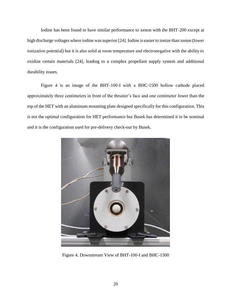
Figure 4 is an image of the BHT-100-I with a BHC-1500 hollow cathode placed

approximately three centimeters in front of the thruster’s face and one centimeter lower than the

top of the HET with an aluminum mounting plate designed specifically for this configuration. This

is not the optimal configuration for HET performance but Busek has determined it to be nominal

and it is the configuration used for pre-delivery check-out by Busek.

Figure 4. Downstream View of BHT-100-I and BHC-1500

21

The BHT-100-I is designed to operate at power levels between 75 and 125 Watts with a

nominal discharge potential between two hundred and three hundred volts. The cathode mass flow

rate may be varied from less than 10% to more than 30% of the anode mass flow rate. The cathode

mass flow rate is known to influence the measured performance and structure of the plume for this

model; divergence and cathode mass flow rate are positively correlated due to collisional

scattering. These devices require the electrical connections depicted in figure 5.

Figure 5. BHT-100-I and BHC-1500 Electrical Diagram

The cathode body is connected to the keeper ground, heater ground, and anode power

supply ground. The body of the thruster is grounded to the vacuum chamber and cathode body

ground through bracket attachment posts and an aluminum mounting plate. The BHT-100-I and

BHC-1500 are stored in a climate-controlled cabinet while not in use and are only handled with

gloves.

2.3 Plasma Fundamentals

HETs generate thrust by ionizing and accelerating a neutral propellant in plasma. Plasma

is the result of dissociation and is a dense collection of charged particles. These particles move in

22

response to generated and applied fields, and the plasma is electrically neutral on average [2]. The

physics defining the simplified behavior of plasma are detailed at present.

2.3.1 Quasi-Neutrality and Debye Length

The property of being approximately electrically neutral on average is known as quasi-

neutrality. Quasi-neutrality occurs because the plasma screens the external electric field. The

external electric field induces plasma polarization and the penetration of the field inside the plasma

exponentially decreases [25]. This property does not exist close to the boundaries and is a decent

assumption when the spatial scale length of the plasma is much larger than the Debye length [2].

The Debye length is mathematically described by equation 26 [2].

𝜆𝐷 = √𝜀0𝑘𝑇𝑒

𝑛0𝑞𝑒2

(26)

The Debye length is the characteristic distance that charges or boundaries are

electrostatically shielded. The same distance is required to compensate the electric field of a

charged particle in the plasma and the Debye length indicates the scale of the plasma neutrality

[25]. If the electron concentration is high and the Debye length is small the electrons and ions will

move as a group such that the diffusion is effectively ambipolar as desired. Conversely, if the

opposite is true the plasma is not quasi-neutral and the electrons and ions will move separately so

their diffusion should not be considered free. Debye length does not depend on the ion temperature

because the ions are unable to establish the quasi-equilibrium Boltzmann distribution and are

assumed to be effectively motionless [25].

23

2.3.2 Maxwell’s Equations

In order to understand how plasma particles move in response to electric and magnetic

fields, an understanding of Maxwell’s equations is required. These four equations describe the

electric and magnetic fields that form from distributions of electric charges and current as well as

how these two fields fluctuate and propagate over time.

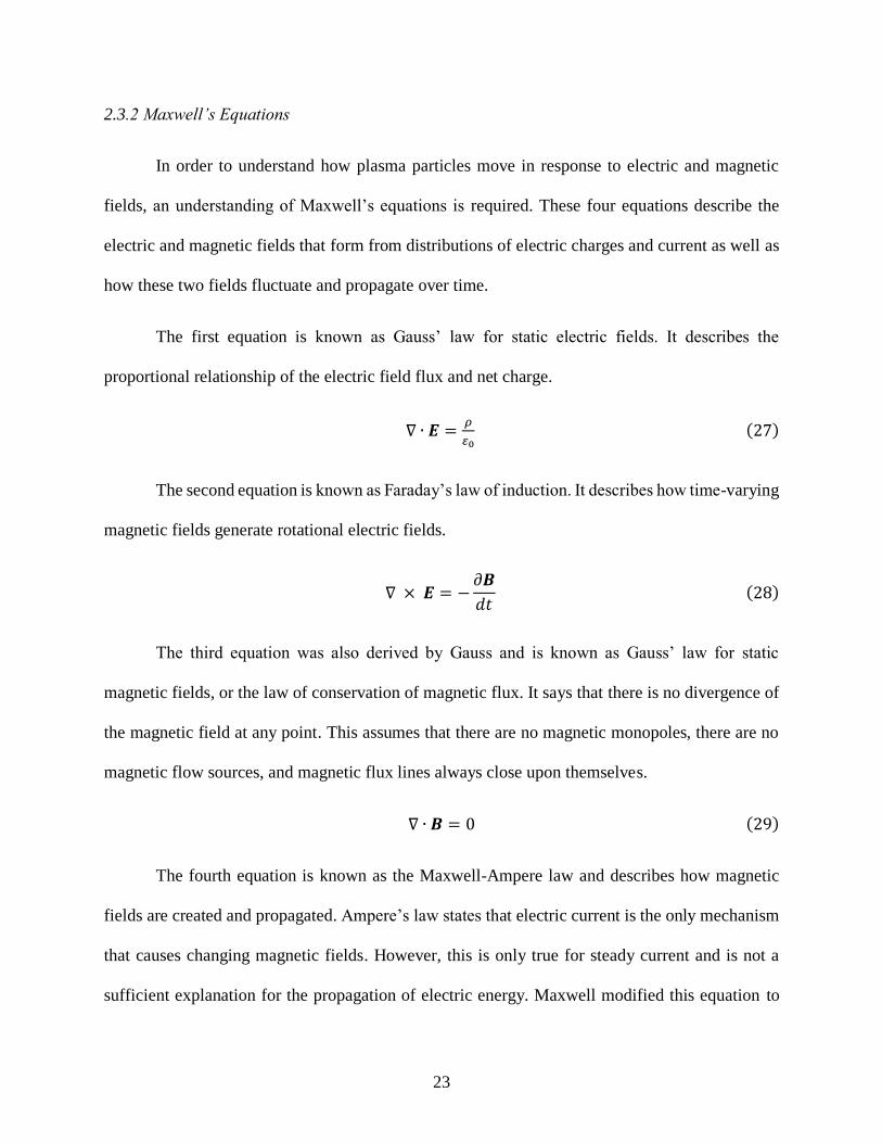
The first equation is known as Gauss’ law for static electric fields. It describes the

proportional relationship of the electric field flux and net charge.

∇ ∙ 𝑬 =𝜌

𝜀0(27)

The second equation is known as Faraday’s law of induction. It describes how time-varying

magnetic fields generate rotational electric fields.

∇ × 𝑬 = −𝜕𝑩

𝑑𝑡(28)

The third equation was also derived by Gauss and is known as Gauss’ law for static

magnetic fields, or the law of conservation of magnetic flux. It says that there is no divergence of

the magnetic field at any point. This assumes that there are no magnetic monopoles, there are no

magnetic flow sources, and magnetic flux lines always close upon themselves.

∇ ∙ 𝑩 = 0 (29)

The fourth equation is known as the Maxwell-Ampere law and describes how magnetic

fields are created and propagated. Ampere’s law states that electric current is the only mechanism

that causes changing magnetic fields. However, this is only true for steady current and is not a

sufficient explanation for the propagation of electric energy. Maxwell modified this equation to

24

account for displacement current, or changing electric fields, as another source of magnetic fields.

This modification to Ampere’s law satisfies the continuity equation of electric charge without

changing the laws for static fields.

∇ × 𝑩 = 𝜇0 ( 𝑱 + 𝜀0

𝜕𝑬

𝜕𝑡) (30)

This set of equations is referred to as Maxwell’s equations because the completed set laid

the foundation for Maxwell’s theory of electromagnetism and provided sufficient explanation for

the relationship between light and electromagnetic waves [26].

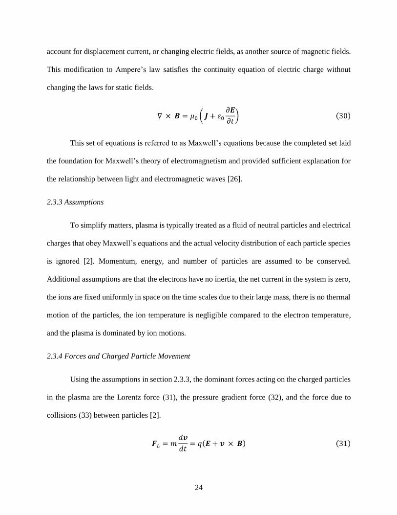
2.3.3 Assumptions

To simplify matters, plasma is typically treated as a fluid of neutral particles and electrical

charges that obey Maxwell’s equations and the actual velocity distribution of each particle species

is ignored [2]. Momentum, energy, and number of particles are assumed to be conserved.

Additional assumptions are that the electrons have no inertia, the net current in the system is zero,

the ions are fixed uniformly in space on the time scales due to their large mass, there is no thermal

motion of the particles, the ion temperature is negligible compared to the electron temperature,

and the plasma is dominated by ion motions.

2.3.4 Forces and Charged Particle Movement

Using the assumptions in section 2.3.3, the dominant forces acting on the charged particles

in the plasma are the Lorentz force (31), the pressure gradient force (32), and the force due to

collisions (33) between particles [2].

𝑭𝐿 = 𝑚𝑑𝒗

𝑑𝑡= 𝑞(𝑬 + 𝒗 × 𝑩) (31)

25

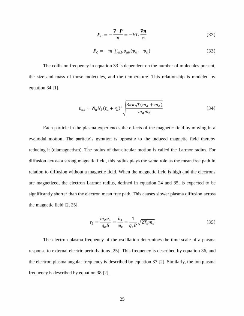
𝑭𝑃 = −∇ ∙ 𝑷

𝑛= −𝑘𝑇𝑒

∇𝒏

𝑛(32)

𝑭𝐶 = −𝑚 ∑ 𝜐𝑎𝑏(𝒗𝑎 − 𝒗𝑏)𝑎,𝑏 (33)

The collision frequency in equation 33 is dependent on the number of molecules present,

the size and mass of those molecules, and the temperature. This relationship is modeled by

equation 34 [1].

𝜐𝑎𝑏 = 𝑁𝑎𝑁𝑏(𝑟𝑎 + 𝑟𝑏)2√8𝜋𝑘𝐵𝑇(𝑚𝑎 + 𝑚𝑏)

𝑚𝑎𝑚𝑏 (34)

Each particle in the plasma experiences the effects of the magnetic field by moving in a

cycloidal motion. The particle’s gyration is opposite to the induced magnetic field thereby

reducing it (diamagnetism). The radius of that circular motion is called the Larmor radius. For

diffusion across a strong magnetic field, this radius plays the same role as the mean free path in

relation to diffusion without a magnetic field. When the magnetic field is high and the electrons

are magnetized, the electron Larmor radius, defined in equation 24 and 35, is expected to be

significantly shorter than the electron mean free path. This causes slower plasma diffusion across

the magnetic field [2, 25].

𝑟𝐿 =𝑚𝑒𝑣⊥

𝑞𝑒𝐵=

𝑣⊥

𝜔𝑐=

1

𝑞𝑒𝐵√2𝑇𝑒𝑚𝑒 (35)

The electron plasma frequency of the oscillation determines the time scale of a plasma

response to external electric perturbations [25]. This frequency is described by equation 36, and

the electron plasma angular frequency is described by equation 37 [2]. Similarly, the ion plasma

frequency is described by equation 38 [2].

26

𝜔𝑝 = √𝑛𝑒𝑞𝑒

2

𝜀0𝑚𝑒 (36)

𝑓𝑝 =𝜔𝑝

2𝜋≈ 9√𝑛𝑒 (37)

Ω𝑝 = √𝑛𝑒𝑞𝑒

2

𝜀0𝑀(38)

The electron plasma density is approximately the inverse of the minimum time required

for the plasma to react to changes in its boundaries or in the applied potentials. It corresponds to

the time a thermal electron travels the Debye length (equation 26) that is needed to provide

screening of the external perturbation [25].

2.3.5 Classical Diffusion

Pressure gradients and collisions between particles produce diffusion of the plasma from

high to low density regions. Diffusion occurs along and across magnetic field lines and is

significant in the particle transport of HET plasmas. This diffusion mechanism is referred to as

classical diffusion theory. Classical diffusion-driven particle motion in plasma is described by the

sum of the three dominant forces listed in equations 31 through 33 and is expressed mathematically

by equation 39.

∑ 𝑭 = 𝑚𝑑𝒗

𝑑𝑡= 𝑞𝑒(𝑬 + 𝒗 × 𝑩) −

∇(𝒏𝑘𝑇𝑒)

𝑛− 𝑚 ∑ 𝜐𝑎𝑏(𝒗𝑎 − 𝒗𝑏)

𝑎,𝑏

(39)

Assuming steady state classical diffusion, the perpendicular electron mobility and

perpendicular classical cross-field diffusion coefficients are defined in equations 40 and 41 [2].

27

𝜇⊥ =𝜇

1 + 𝜔𝑐2𝜏2

=𝜇

1 + Ω𝑒2

(40)

D⊥ = D

1 + ωc2τ2

=D

1 + 𝛺e2

(41)

The perpendicular velocity is a form of Fick’s law with additional azimuthal electric and

magnetic field cross drift (equation 42) and diamagnetic drift terms (equation 43). This is described

by equation 44 [2].

𝒗𝐸 = 𝑬 × 𝑩

𝐵02 (42)

𝒗𝐷 = −𝑘𝑇𝑒

𝑞𝑒𝐵02

∇𝑛 × 𝑩

𝑛 (43)

𝒗⊥ = ±𝜇⊥𝐸 − 𝐷⊥

∇𝑛

𝑛+

𝒗𝐸 + 𝒗𝐷

1 + 𝜐2 𝜔𝑐2⁄

(44)

The perpendicular cross-field electron flux flowing towards the anode is similarly

described by Fick’s law, with additional coefficients due to the magnetic field. This perpendicular

flux is described by equation 45 [2].

𝚪𝑒 = 𝑛𝒗⊥ = ±𝜇⊥𝑛𝑬 − 𝐷⊥∇𝑛 (45)

2.3.6 Plasma Oscillations

HET plasma has a variety of complex wave and noise characteristics over a wide frequency

spectrum. These oscillations are important to understand and characterize because they can affect

the divergence of the ion beam, performance level, and efficiency of HETs [11]. This is because

many of the oscillations are inherent to the ionization, particle diffusion, and acceleration processes

previously described [11]. The oscillations are excited by the plasma to self-regulate the charged

28

particle production and diffusion processes while adjusting to the imposed operating mode. These

oscillations range from broadband turbulence to narrow-band, distinct waves.

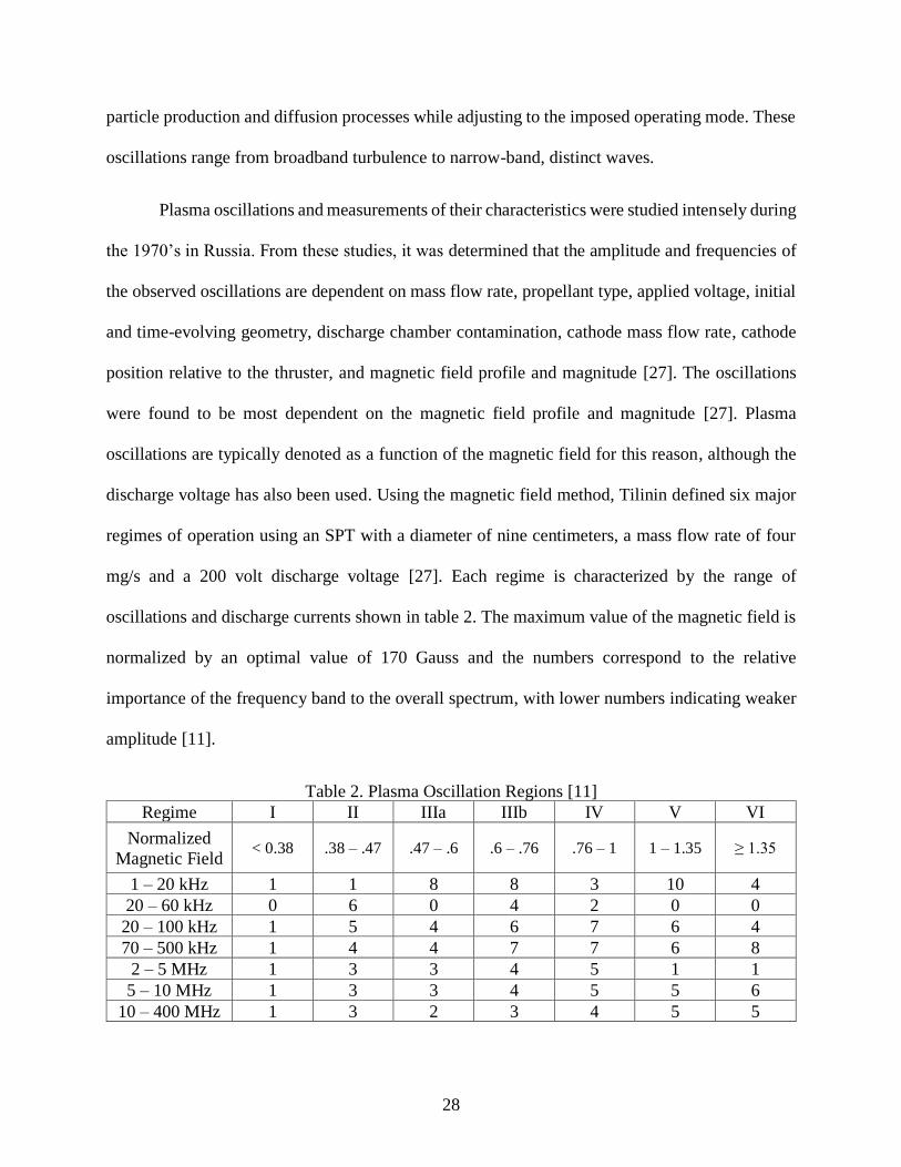
Plasma oscillations and measurements of their characteristics were studied intensely during

the 1970’s in Russia. From these studies, it was determined that the amplitude and frequencies of

the observed oscillations are dependent on mass flow rate, propellant type, applied voltage, initial

and time-evolving geometry, discharge chamber contamination, cathode mass flow rate, cathode

position relative to the thruster, and magnetic field profile and magnitude [27]. The oscillations

were found to be most dependent on the magnetic field profile and magnitude [27]. Plasma

oscillations are typically denoted as a function of the magnetic field for this reason, although the

discharge voltage has also been used. Using the magnetic field method, Tilinin defined six major

regimes of operation using an SPT with a diameter of nine centimeters, a mass flow rate of four

mg/s and a 200 volt discharge voltage [27]. Each regime is characterized by the range of

oscillations and discharge currents shown in table 2. The maximum value of the magnetic field is

normalized by an optimal value of 170 Gauss and the numbers correspond to the relative

importance of the frequency band to the overall spectrum, with lower numbers indicating weaker

amplitude [11].

Table 2. Plasma Oscillation Regions [11]

Regime I II IIIa IIIb IV V VI

Normalized

Magnetic Field < 0.38 .38 – .47 .47 – .6 .6 – .76 .76 – 1 1 – 1.35 ≥ 1.35

1 – 20 kHz 1 1 8 8 3 10 4

20 – 60 kHz 0 6 0 4 2 0 0

20 – 100 kHz 1 5 4 6 7 6 4

70 – 500 kHz 1 4 4 7 7 6 8

2 – 5 MHz 1 3 3 4 5 1 1

5 – 10 MHz 1 3 3 4 5 5 6

10 – 400 MHz 1 3 2 3 4 5 5

29

The fourth regime is referred to as the optimal regime because the oscillations are damped

in comparison to the other regions. The oscillations in this regime may be described by a predator-

prey model and the primary origin of these oscillations is well known. The oscillations are caused

by a periodic depletion and replenishment of the neutral near the exit. Enhanced ionization depletes

the neutral density and causes a downstream front of the neutral flow to move upstream into an

area where the ionization rate is lower. The decrease in upstream ionization rate causes a decrease

in the flux of electrons to the exit, leading the ionization in that region to abate and bring the

downstream neutral gas front back down where the cycle restarts. This oscillation occurs on the

time scale of the neutral replenishment time [2] and the oscillation cycle is referred to as a

breathing oscillation because it appears as if the thruster is breathing when the front moves closer

to and farther away from the thruster’s face. This oscillation impacts the discharge current because

the ion density oscillations impact electron conductivity through the transverse magnetic field [28].

2.4 Plasma Instabilities and Anomalous Diffusion Mechanisms

The classical cross-field diffusion coefficient is proportional to 1

𝐵2 and does not match

measured data. Experimental results indicate electron conductivity one to two orders of magnitude

greater than expected by classical diffusion theory mechanisms inside of the channel and plume

[29]. Anomalous diffusion refers to this electron current that is significantly higher than expected.

It is the result of mechanisms believed to modify electron dynamics to reduce their resistivity,

although there is disagreement and uncertainty about what these mechanisms are.

Anomalous diffusion is believed to be present in the entire thruster channel and plume

although the processes may be completely different in each. Experimental results indicate electron

conductivity is higher in the near-field plume than in the channel, there is lower conductivity in

30

the region of high magnetic and electric fields, magnetic field topology affects electron

conductivity, and electron mobility is proportional to 1

𝐵 instead of

1

𝐵2 [14].

2.4.1 Bohm Diffusion

Bohm diffusion is one of the two most commonly proposed anomalous transport

mechanisms. Experimental results are more closely described by the Bohm diffusion coefficient

(proportional to 1

𝐵). Bohm diffusion most likely dominates anomalous diffusion at low-voltages

because the electron temperature is lower, thereby reducing the wall collision rate [30]. It has been

experimentally found to dominate near the anode and downstream of the exit plane [8]. Bohm

diffusion is thought to be the result of collective plasma drift instabilities, where correlated

oscillations of the electric and density fields induce a net axial electron current [29]. This theory

was originally proposed by Bohm, and later derived by Spitzer in 1960 by assuming the existence

of homogenous turbulence in the plasma leading to diffusion [31]. It is empirically estimated by

equation 46.

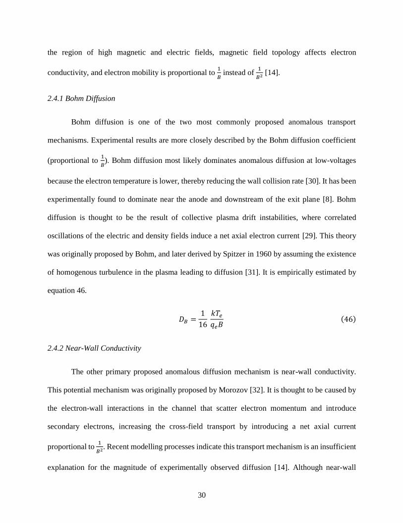
𝐷𝐵 =1

16 𝑘𝑇𝑒

𝑞𝑒𝐵(46)

2.4.2 Near-Wall Conductivity

The other primary proposed anomalous diffusion mechanism is near-wall conductivity.

This potential mechanism was originally proposed by Morozov [32]. It is thought to be caused by

the electron-wall interactions in the channel that scatter electron momentum and introduce

secondary electrons, increasing the cross-field transport by introducing a net axial current

proportional to 1

𝐵2. Recent modelling processes indicate this transport mechanism is an insufficient

explanation for the magnitude of experimentally observed diffusion [14]. Although near-wall

31

conductivity may contribute to diffusion, it cannot be the only mechanism contributing to

anomalous diffusion. It is likely Bohm diffusion and near-wall conductivity both contribute to

anomalous diffusion although they play a role in different regions of the thruster and are dominant

at different operating conditions [8].

2.4.3 Rotating Spokes

A high-frequency phenomenon referred to as the rotating spoke is believed to be caused by

an additional anomalous diffusion mechanism. It was first observed in 1966 by Janes and Lowder,

who were also the first to correlate the in-phase azimuthal electric field fluctuations with density

gradients. Janes and Lowder suggested rotating spokes could be the result of an additional

anomalous diffusion mechanism via the crossed electric and magnetic fields that causes an increase

in net electron transport to the anode [15].

Another proposed theory for the mechanism causing the rotating spokes is that the observed

spokes are the result of incomplete gas ionization and the rapid loss of newly disassociated ions

[33]. Newer theories include the existence of plasma waves where the spokes’ presence indicates

breathing-mode damping, localized breathing modes that exhibit an azimuthally local discharge

and replenishment process similar to HET breathing modes, and wall heating [34].

Regardless of the actual mechanism causing the observed spokes, the diffusion associated

with the rotating spokes scales as the inverse of the magnetic field, similar to Bohm diffusion [8].

Experimental results suggest the velocity is correlated with the first ionization potential of the

neutral gas, indicating a close connection between the ionization process and the appearance of the

spokes [14]. Additionally, Lomas and Kilkenny observed that the phase speed of the spokes

increases with the magnetic field, and more recent experiments suggest that the cathode influences

32

the spokes and electron conductivity [35]. This is a continued field of study because although the

intensity makes it reasonable to suggest a relation with increased diffusion, the physics detailing

this plasma behavior are complex and poorly understood [13]. The location in the plasma the

spokes are formed in is still unknown as well as the mechanism explaining their onset [13].

2.5 Faraday Probe

A Faraday probe is an intrusive device that measures ions in the plume with a uniform

collector plate to evaluate the divergence angle of the plume and the beam’s current density profile.

For this experiment, this is accomplished by radially sweeping the thruster’s plume at varying

distances.

The Faraday probe measures a drop in voltage at the collector plate due to a change in

current from ion bombardment. The area of the Faraday probe’s aperture and the resistance of the

plate are known values. The local beam current density may be solved for using these known

values and the measured drop in voltage, using Ohm’s law to solve for the current and then dividing

by the area of the aperture. This provides a single current density for one point of the plume. The

process for calculating the current density is mathematically by equation 47 [36].

𝐽𝑏 =𝑉𝑑𝑟𝑜𝑝/𝑅𝑝𝑙𝑎𝑡𝑒

𝐴𝑎𝑝𝑒𝑟𝑡𝑢𝑟𝑒 (47)

Equation 47 assumes the plasma originates from a single point source located at the center

of the HET. However, the channel is a more accurate location of ion production than the center of

the HET [37], meaning there are two point sources for each radial sweep of the plume. Equation

47 must be modified to account for the HET’s geometry and the cosine losses associated with that

geometry. This is accomplished by accounting for the distance between the point sources and

33

correcting the angle to each point source [21]. Figure 6 is a diagram depicting all of the distances

and angles needed to compute the correction factors.

Figure 6. Faraday Probe Geometry to Thruster

The area correction factor accounts for difference in the angles from the probe orifice to

the center of each channel (equation 48). These variations affect the current collection area by the

factor mathematically described by equation 49 [21]. The cosine losses are averaged between the

two point sources.

𝛼𝐿,𝑅 = ± (𝜋 − 𝜃 − tan−1 (cos 𝜃 ∓

𝑅𝐶𝐿𝑅

sin 𝜃)) (48)

𝜅𝐴 = cos2 (𝛼𝐿 + 𝛼𝑅

2) (49)

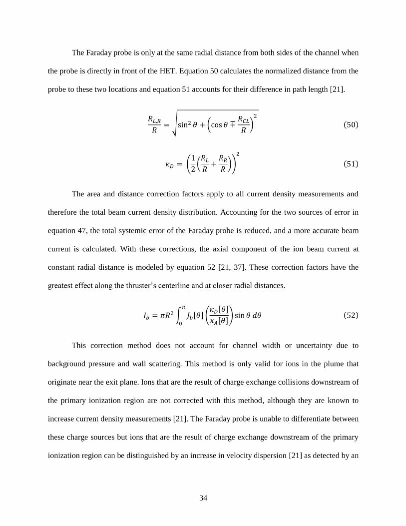
34

The Faraday probe is only at the same radial distance from both sides of the channel when

the probe is directly in front of the HET. Equation 50 calculates the normalized distance from the

probe to these two locations and equation 51 accounts for their difference in path length [21].

𝑅𝐿,𝑅

𝑅= √sin2 𝜃 + (cos 𝜃 ∓

𝑅𝐶𝐿

𝑅)

2

(50)

𝜅𝐷 = (1

2(

𝑅𝐿

𝑅+

𝑅𝑅

𝑅))

2

(51)

The area and distance correction factors apply to all current density measurements and

therefore the total beam current density distribution. Accounting for the two sources of error in

equation 47, the total systemic error of the Faraday probe is reduced, and a more accurate beam

current is calculated. With these corrections, the axial component of the ion beam current at

constant radial distance is modeled by equation 52 [21, 37]. These correction factors have the

greatest effect along the thruster’s centerline and at closer radial distances.

𝐼𝑏 = 𝜋𝑅2 ∫ 𝐽𝑏[𝜃] (𝜅𝐷[𝜃]

𝜅𝐴[𝜃]) sin 𝜃 𝑑𝜃

𝜋

0

(52)

This correction method does not account for channel width or uncertainty due to

background pressure and wall scattering. This method is only valid for ions in the plume that

originate near the exit plane. Ions that are the result of charge exchange collisions downstream of

the primary ionization region are not corrected with this method, although they are known to

increase current density measurements [21]. The Faraday probe is unable to differentiate between

these charge sources but ions that are the result of charge exchange downstream of the primary

ionization region can be distinguished by an increase in velocity dispersion [21] as detected by an

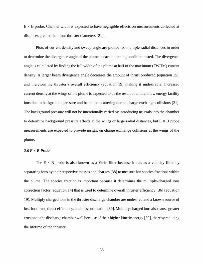
35

E × B probe. Channel width is expected to have negligible effects on measurements collected at

distances greater than four thruster diameters [21].

Plots of current density and sweep angle are plotted for multiple radial distances in order

to determine the divergence angle of the plume at each operating condition tested. The divergence

angle is calculated by finding the full width of the plume at half of the maximum (FWHM) current

density. A larger beam divergence angle decreases the amount of thrust produced (equation 15),

and therefore the thruster’s overall efficiency (equation 19) making it undesirable. Increased

current density at the wings of the plume is expected to be the result of ambient low energy facility

ions due to background pressure and beam ion scattering due to charge exchange collisions [21].

The background pressure will not be intentionally varied by introducing neutrals into the chamber

to determine background pressure effects at the wings or large radial distances, but E × B probe

measurements are expected to provide insight on charge exchange collisions at the wings of the

plume.

2.6 E × B Probe

The E × B probe is also known as a Wein filter because it acts as a velocity filter by

separating ions by their respective masses and charges [38] to measure ion species fractions within

the plume. The species fraction is important because it determines the multiply-charged ions

correction factor (equation 14) that is used to determine overall thruster efficiency [36] (equation

19). Multiply charged ions in the thruster discharge chamber are undesired and a known source of

loss for thrust, thrust efficiency, and mass utilization [39]. Multiply charged ions also cause greater

erosion to the discharge chamber wall because of their higher kinetic energy [39], thereby reducing

the lifetime of the thruster.

36

The E × B probe records the velocity of the ions it collects as a function of the charge state

through the use of the Lorentz force equation expressed in equation 53 [36, 38].

𝑭𝑖 = 𝑞𝑖(𝑬 + 𝒗𝑖 × 𝑩) (53)

The Lorentz equation describes the force acting on a charged particle moving within an

electric and magnetic field. In order for the E × B probe to collect the ion and produce a current,

the ion must be able to pass through the probe to the collector plate depicted in figure 7.

Figure 7. Electric and Magnetic Fields within E × B Probe

The ion will only reach the output collimator if it is not pushed off the drift axis. This will

occur when there is no net force acting on the ion, or when equation 53 is set to zero. The velocity

of an ion that will not be pushed off the drift axis when it enters the probe is portrayed by equation

54 (neglecting initial thermal velocities) [38].

𝑣𝑖 = −𝐸

𝐵= √

2𝑧𝑞𝑖Δ𝑉𝑖

𝑚𝑖 (54)

The probe’s plate voltage difference is swept over a range of values while the distance

between the plates and the magnetic field are held constant. This method separates each ion

according to its mass, charge state, and the potential difference between the ion creation point in

37

the plasma and the entrance collimator of the probe. This is visually depicted as a series of

decreasing peaks of current as the voltage to the bias plates is increased. Each successive peak

corresponds to an increased ionization state. The equation for the ions that are measured by the

probe is given by equation 55 [36].

∆𝜙 = 𝐵𝑑√2𝑧𝑞𝑖Δ𝑉𝑖

𝑚𝑖 (55)

The ions able to impact the collector plate because they are not deflected by the induced

electric field yield a current. When the current is plotted as a function of the plate bias voltage

distinct peaks of decreasing height and decreased area under the curve are expected. These peaks

represent the relative species concentrations within the plume and are correlated with singly

through multiply charged ions. The beam current fraction and ion species fraction are calculated

using the relationships mathematically described by equations 56 and 57 [36, 38, 40].

Ω𝑖 =𝑛𝑖𝑞

𝑖

32

∑ 𝑛𝑖𝑞𝑖

32

=𝐼𝑖

∑ 𝐼𝑖 , 𝑖 = 1,2,3 (56)

𝜁𝑖 =𝑛𝑖

∑ 𝑛𝑖 =

Ω𝑖 𝑞𝑖

32⁄

∑ Ω𝑖 𝑞𝑖

32⁄

, 𝑖 = 1,2,3 (57)

The multiply charged ions present in HET plumes are the result of multiple collisions or a

single collision with a more energetic electron. Data from previous experiments suggests potential

collisions within the plume and probe in addition to the thruster channel [38]. Previous experiments

also suggest multiply charged ions are created further downstream and at higher angles from the

thruster exit plane due to discharge chamber geometry and a secondary ionization region [38]. Ion

38

behavior at higher angles is very important behavior to understand and characterize in order to

limit erosion rates on spacecraft surfaces.

2.7 Emissive Probe

The emissive probe is an intrusive device that measures the potential of the plasma. It is a

viable device to study HET plumes because the plume is a moving stream of plasma that carries

electric fields and potentials and therefore localized charge distributions. This makes the local

plasma potential in the plume a useful diagnostic measurement for determining the electron and

ion populations within the plume [12] and for observing changes in ionization when the rotating

spokes are present.

For this research, the probe potential is allowed to vary freely relative to ground through

the use of a large load resistor. This method was developed by Kemp and Sellen in 1966 [12] and

is the method used because the emissive probe is meant to take time-synchronous data of the

induced rotating spokes at high sampling rates with the oscilloscope and high-speed camera. Using

this method, the current in the load resistor will be used to determine the potential drop at the

center of the probe filament. It is a good estimate of the potential as long as the natural logarithm

of (𝐼𝑠,𝑐

𝐼𝑠,𝑖+𝐼𝑒,𝑒) is greater than one. The potential is expressed mathematically by equation 58 [12].

𝑉𝑓 = 𝑉𝑝 − 𝑇𝑒 ln (𝐼𝑠,𝑐

𝐼𝑠,𝑖 + 𝐼𝑒,𝑒) (58)

Although the emissive probe provides a direct measurement of the plasma potential, it is

not insusceptible to error. The main sources of concern are the voltage drop across the filament

from the heating power supply and the difference between the true plasma potential and the heated

probe’s potential. Although the probe floats near the true potential, it is commonly accepted that a

39

sufficiently heated probe can still float below the true potential by about 1.03 times the electron

temperature [41]. This is expected to affect all measurements similarly so that the change in plasma

potential over time is uniformly affected.

40

III. Setup and Methodology

All experiments for this research take place in the Air Force Institute of Technology’s

Space Propulsion Application Simulation System Laboratory vacuum chamber at Wright-

Patterson Air Force Base, Ohio.

Testing begins by verifying the BHT-100-I operates as expected by comparing measured

discharge voltage and current, mass flow rates, and magnet voltage and current to pre-delivery

check-out data provided by Busek. The resistance across the inner magnetic coil will also be

measured and compared to the bench test data provided by Busek.

Thruster operation will then be characterized using a Faraday probe and an E × B probe.

The Faraday probe measures ion current in the plume and is used to calculate the plume’s current

density and divergence angle when conducted across a radial sweep of the plume. The E × B probe

measures ion species fractions. Both of these devices examine exhaust plume properties across the

nominal operating ranges of the BHT-100-I in order to determine and characterize the optimal

operating range for highest efficiency, highest single ionization, and smallest divergence angle of

the plume. Radial sweeps of the plume are independently conducted with these devices at 20, 30,

40, and 50 centimeters from the thruster face in one degree increments with a five second dwell

time per angle.

The thruster then runs at full power with a nominal discharge potential and anode mass

flow rate so that the plume has suppressed azimuthal features as observed by the time-synchronous

emissive probe, oscilloscope, and high-speed camera. The emissive probe measures the local

potential of the plasma, the oscilloscope measures discharge current, and the high-speed camera

measures the relative brightness across the channel. The discharge voltage is then decreased by at

41

least 50% and the anode mass flow rate is increased up to 10% in order to observe density

instabilities and azimuthal oscillations while maintaining overall stability at a higher discharge

current. The emissive probe and high-speed camera are used concurrently to observe the rotating

spokes phenomenon at frequencies between 125 kHz and one MHz. This phenomenon is not

expected to be observable at frequencies below this range.

3.1 Vacuum Chamber

The SPASS vacuum chamber was manufactured and installed by PHPK Technologies,

located in Columbus, Ohio [36] and its primary use is to aid in the research of electric propulsion

thrusters at AFIT. The vacuum chamber is cylindrical with a 1.8 meter diameter and 3.75 meter

length. The interior is composed of 304 stainless steel with a number four finish. There are seven

ports along the exterior of the chamber that house 25 centimeter diameter quartz windows for

visual observation and high-speed image data collection. Contamination occurs on the windows

from the deposition of eroded steel and aluminum from the chamber and structures within the

chamber. The amount of build-up on the window prior to testing is not great enough to affect the

relative brightness of the channel as observed by the images taken with the high-speed camera and

therefore does not necessitate removal and polishing prior to testing.

42

Figure 8. SPASS Vacuum Chamber

3.1.1 Pumping System

The vacuum chamber is capable of maintaining a pressure of 10-8 Torr while the thrusters

are off and around 10-6 Torr during thruster operation using a two-staged pump system [36].

The first stage of the two-staged pumping system is a dry compressing pump procedure

that mechanically pumps atmospheric air out of the chamber using a Screwline 250 pump pictured

in figure 9. It operates using the screw principle, where the pumping chamber is formed by two

synchronized positive displacement rotors that rotate in opposite directions [42]. At 60 Hertz, the

SP250 has a pumping speed of 330 cubic meters per hour with an ultimate pressure of

approximately 7.5 millitorr.

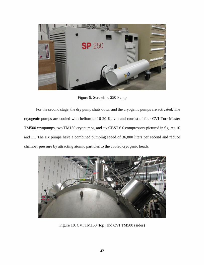
43

Figure 9. Screwline 250 Pump

For the second stage, the dry pump shuts down and the cryogenic pumps are activated. The

cryogenic pumps are cooled with helium to 16-20 Kelvin and consist of four CVI Torr Master

TM500 cryopumps, two TM150 cryopumps, and six CBST 6.0 compressors pictured in figures 10

and 11. The six pumps have a combined pumping speed of 36,800 liters per second and reduce

chamber pressure by attracting atomic particles to the cooled cryogenic heads.

Figure 10. CVI TM150 (top) and CVI TM500 (sides)

44

Figure 11. CBST 6.0 Compressors

The overall pressure is monitored by a Kurt J. Lesker Company Pirani gauge when the

pressures is greater than one millitorr and by ExTorr’s Residual Gas Analyzer (RGA) Vacuum

Plus software when the pressure is below one millitorr [12]. ExTorr’s RGA Vacuum Plus software

also measures the partial pressures of constituent species. It has a scanning speed of 144 Hertz and

looks for species below 110 amu. Species greater than 110 amu will be observed by the sensor but

the mass will be inaccurate due to sensor limitations and aliasing effects (xenon is 131.3 amu but

corresponds to a spike at 63 amu). The RGA has a total sensitivity of 1 per Torr and a partial

sensitivity of 6 × 10-4 per Torr. The user interface depicted in figure 12 may be scaled as needed.

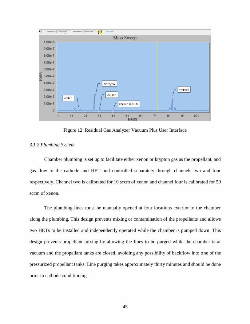
45

Figure 12. Residual Gas Analyzer Vacuum Plus User Interface

3.1.2 Plumbing System

Chamber plumbing is set up to facilitate either xenon or krypton gas as the propellant, and

gas flow to the cathode and HET and controlled separately through channels two and four

respectively. Channel two is calibrated for 10 sccm of xenon and channel four is calibrated for 50

sccm of xenon.

The plumbing lines must be manually opened at four locations exterior to the chamber

along the plumbing. This design prevents mixing or contamination of the propellants and allows

two HETs to be installed and independently operated while the chamber is pumped down. This

design prevents propellant mixing by allowing the lines to be purged while the chamber is at

vacuum and the propellant tanks are closed, avoiding any possibility of backflow into one of the

pressurized propellant tanks. Line purging takes approximately thirty minutes and should be done

prior to cathode conditioning.

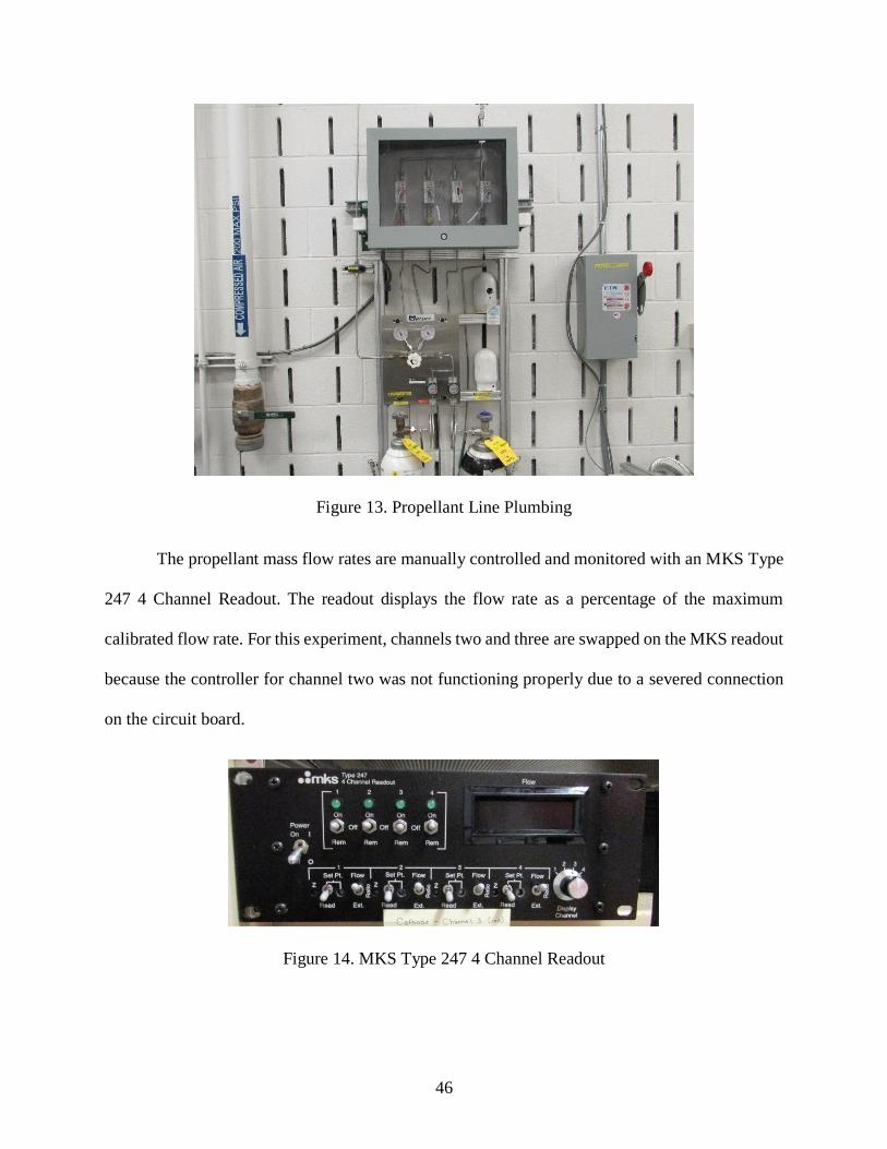
46

Figure 13. Propellant Line Plumbing

The propellant mass flow rates are manually controlled and monitored with an MKS Type

247 4 Channel Readout. The readout displays the flow rate as a percentage of the maximum

calibrated flow rate. For this experiment, channels two and three are swapped on the MKS readout

because the controller for channel two was not functioning properly due to a severed connection

on the circuit board.

Figure 14. MKS Type 247 4 Channel Readout

47

In order to bring the SPASS vacuum chamber back up to atmospheric pressure safely,

additional plumbing exists to manually flow nitrogen into the chamber. Nitrogen is used because

it is an inexpensive and nonreacting molecule that will not poison the cathode insert. This process

takes several hours to complete and should not be started until several hours after HET operation

has ended to ensure all components have cooled.

3.2 Test Setup

The BHT-100-I is mounted to a fixed frame at the far end of the vacuum chamber roughly

1.4 meters from the rear door and centered within the chamber such that the BHT’s face lines up

with the center of the window it faces. This is accomplished with a u-shaped frame made of

aluminum 80/20 T-slots and fasteners attached to an existing rack within the chamber. The frame

is attached in a way that does not interfere with traverse operation. Figure 15 depicts this setup.

Figure 15. Test Setup Diagram

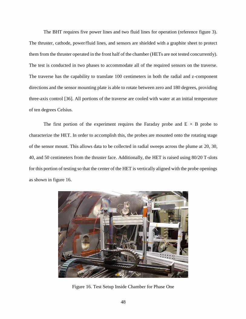
48

The BHT requires five power lines and two fluid lines for operation (reference figure 3).

The thruster, cathode, power/fluid lines, and sensors are shielded with a graphite sheet to protect

them from the thruster operated in the front half of the chamber (HETs are not tested concurrently).

The test is conducted in two phases to accommodate all of the required sensors on the traverse.

The traverse has the capability to translate 100 centimeters in both the radial and z-component

directions and the sensor mounting plate is able to rotate between zero and 180 degrees, providing

three-axis control [36]. All portions of the traverse are cooled with water at an initial temperature

of ten degrees Celsius.

The first portion of the experiment requires the Faraday probe and E × B probe to

characterize the HET. In order to accomplish this, the probes are mounted onto the rotating stage

of the sensor mount. This allows data to be collected in radial sweeps across the plume at 20, 30,

40, and 50 centimeters from the thruster face. Additionally, the HET is raised using 80/20 T-slots

for this portion of testing so that the center of the HET is vertically aligned with the probe openings

as shown in figure 16.

Figure 16. Test Setup Inside Chamber for Phase One

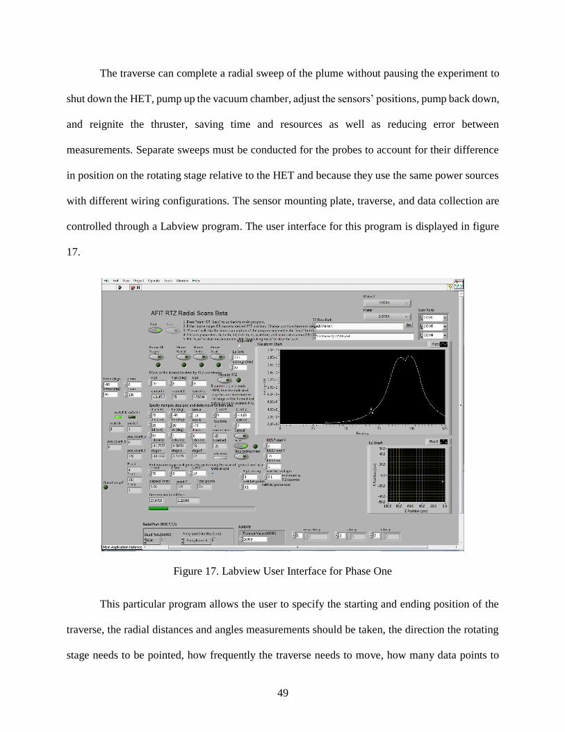
49

The traverse can complete a radial sweep of the plume without pausing the experiment to

shut down the HET, pump up the vacuum chamber, adjust the sensors’ positions, pump back down,

and reignite the thruster, saving time and resources as well as reducing error between

measurements. Separate sweeps must be conducted for the probes to account for their difference

in position on the rotating stage relative to the HET and because they use the same power sources

with different wiring configurations. The sensor mounting plate, traverse, and data collection are

controlled through a Labview program. The user interface for this program is displayed in figure

17.

Figure 17. Labview User Interface for Phase One

This particular program allows the user to specify the starting and ending position of the

traverse, the radial distances and angles measurements should be taken, the direction the rotating

stage needs to be pointed, how frequently the traverse needs to move, how many data points to

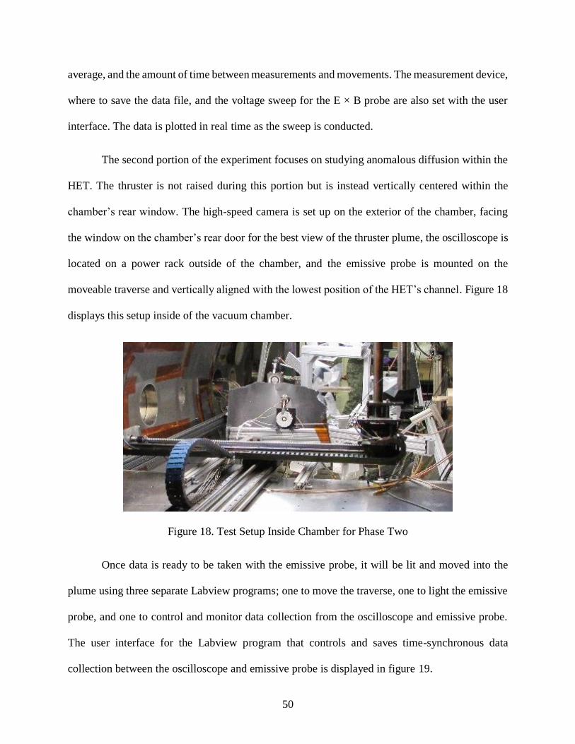
50

average, and the amount of time between measurements and movements. The measurement device,

where to save the data file, and the voltage sweep for the E × B probe are also set with the user

interface. The data is plotted in real time as the sweep is conducted.

The second portion of the experiment focuses on studying anomalous diffusion within the

HET. The thruster is not raised during this portion but is instead vertically centered within the

chamber’s rear window. The high-speed camera is set up on the exterior of the chamber, facing

the window on the chamber’s rear door for the best view of the thruster plume, the oscilloscope is

located on a power rack outside of the chamber, and the emissive probe is mounted on the

moveable traverse and vertically aligned with the lowest position of the HET’s channel. Figure 18

displays this setup inside of the vacuum chamber.

Figure 18. Test Setup Inside Chamber for Phase Two

Once data is ready to be taken with the emissive probe, it will be lit and moved into the

plume using three separate Labview programs; one to move the traverse, one to light the emissive

probe, and one to control and monitor data collection from the oscilloscope and emissive probe.

The user interface for the Labview program that controls and saves time-synchronous data

collection between the oscilloscope and emissive probe is displayed in figure 19.

51

Figure 19. Labview User Interface for Phase Two

The emissive probe will not be lit or moved into the plume until data is ready to be taken

in an effort to increase data collection time before the exposed tungsten wire inevitably breaks.

3.3 Thruster Operation

The HET and cathode are manually controlled and monitored with four separate power

supplies. The cathode heater is controlled with a Sorensen DCS33-33E power supply. This supply

is capable of delivering up to 33 volts and 33 amps of current to within 0.1% accuracy with 10 mA

ripples [43]. The heater is controlled while the power supply is in constant current mode. The

cathode keeper and thruster discharge are powered with two separate Matsusada REK650-2.5

power supplies. This type of power supply is able to output up to 650 volts and 2.5 amps. It has a

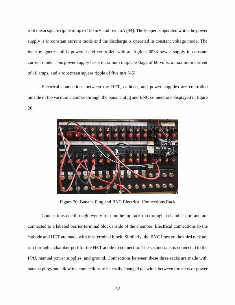
52

root mean square ripple of up to 150 mV and five mA [44]. The keeper is operated while the power

supply is in constant current mode and the discharge is operated in constant voltage mode. The

inner magnetic coil is powered and controlled with an Agilent 6038 power supply in constant

current mode. This power supply has a maximum output voltage of 60 volts, a maximum current

of 10 amps, and a root mean square ripple of five mA [45].

Electrical connections between the HET, cathode, and power supplies are controlled

outside of the vacuum chamber through the banana plug and BNC connections displayed in figure

20.

Figure 20. Banana Plug and BNC Electrical Connections Rack

Connections one through twenty-four on the top rack run through a chamber port and are

connected to a labeled barrier terminal block inside of the chamber. Electrical connections to the

cathode and HET are made with this terminal block. Similarly, the BNC lines on the third rack are

run through a chamber port for the HET anode to connect to. The second rack is connected to the

PPU, manual power supplies, and ground. Connections between these three racks are made with

banana plugs and allow the connections to be easily changed to switch between thrusters or power

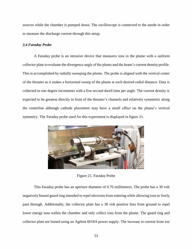
53

sources while the chamber is pumped down. The oscilloscope is connected to the anode in order

to measure the discharge current through this setup.

3.4 Faraday Probe

A Faraday probe is an intrusive device that measures ions in the plume with a uniform

collector plate to evaluate the divergence angle of the plume and the beam’s current density profile.

This is accomplished by radially sweeping the plume. The probe is aligned with the vertical center

of the thruster as it makes a horizontal sweep of the plume at each desired radial distance. Data is

collected in one degree increments with a five second dwell time per angle. The current density is

expected to be greatest directly in front of the thruster’s channels and relatively symmetric along

the centerline although cathode placement may have a small effect on the plume’s vertical

symmetry. The Faraday probe used for this experiment is displayed in figure 21.

Figure 21. Faraday Probe

This Faraday probe has an aperture diameter of 0.76 millimeters. The probe has a 30 volt

negatively biased guard ring intended to repel electrons from entering while allowing ions to freely

pass through. Additionally, the collector plate has a 30 volt positive bias from ground to repel

lower energy ions within the chamber and only collect ions from the plume. The guard ring and

collector plate are biased using an Agilent 6018A power supply. The increase in current from ion

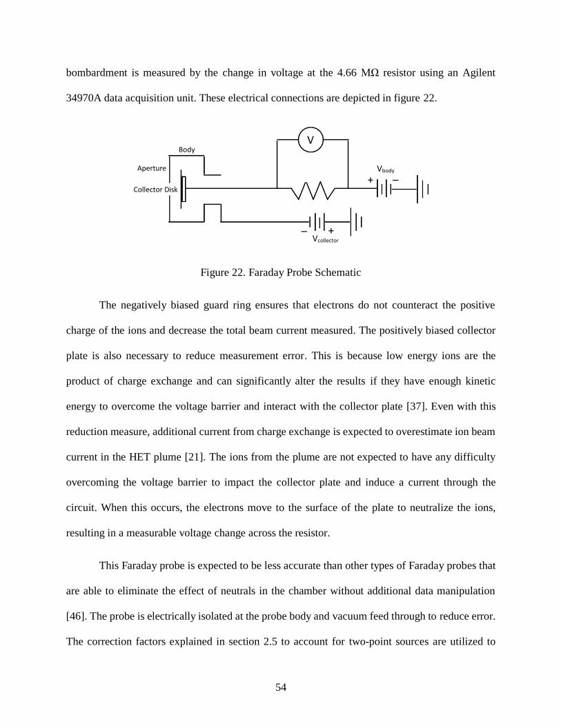
54

bombardment is measured by the change in voltage at the 4.66 MΩ resistor using an Agilent

34970A data acquisition unit. These electrical connections are depicted in figure 22.

Figure 22. Faraday Probe Schematic

The negatively biased guard ring ensures that electrons do not counteract the positive

charge of the ions and decrease the total beam current measured. The positively biased collector

plate is also necessary to reduce measurement error. This is because low energy ions are the

product of charge exchange and can significantly alter the results if they have enough kinetic

energy to overcome the voltage barrier and interact with the collector plate [37]. Even with this

reduction measure, additional current from charge exchange is expected to overestimate ion beam

current in the HET plume [21]. The ions from the plume are not expected to have any difficulty

overcoming the voltage barrier to impact the collector plate and induce a current through the

circuit. When this occurs, the electrons move to the surface of the plate to neutralize the ions,

resulting in a measurable voltage change across the resistor.

This Faraday probe is expected to be less accurate than other types of Faraday probes that

are able to eliminate the effect of neutrals in the chamber without additional data manipulation

[46]. The probe is electrically isolated at the probe body and vacuum feed through to reduce error.

The correction factors explained in section 2.5 to account for two-point sources are utilized to

Aperture

Collector Disk

Body V

Vcollector

Vbody

+

+

_

_

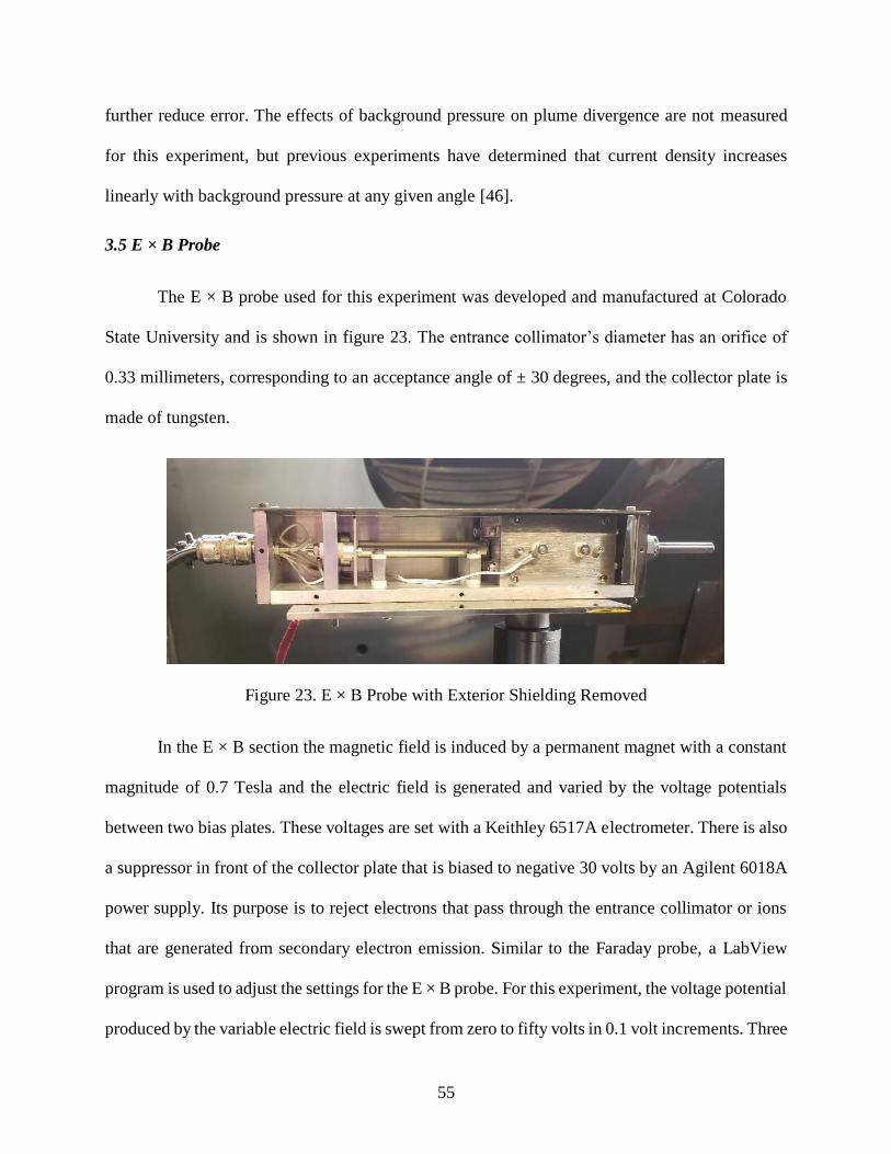
55

further reduce error. The effects of background pressure on plume divergence are not measured

for this experiment, but previous experiments have determined that current density increases

linearly with background pressure at any given angle [46].

3.5 E × B Probe

The E × B probe used for this experiment was developed and manufactured at Colorado

State University and is shown in figure 23. The entrance collimator’s diameter has an orifice of

0.33 millimeters, corresponding to an acceptance angle of ± 30 degrees, and the collector plate is

made of tungsten.

Figure 23. E × B Probe with Exterior Shielding Removed

In the E × B section the magnetic field is induced by a permanent magnet with a constant

magnitude of 0.7 Tesla and the electric field is generated and varied by the voltage potentials

between two bias plates. These voltages are set with a Keithley 6517A electrometer. There is also

a suppressor in front of the collector plate that is biased to negative 30 volts by an Agilent 6018A

power supply. Its purpose is to reject electrons that pass through the entrance collimator or ions

that are generated from secondary electron emission. Similar to the Faraday probe, a LabView

program is used to adjust the settings for the E × B probe. For this experiment, the voltage potential

produced by the variable electric field is swept from zero to fifty volts in 0.1 volt increments. Three

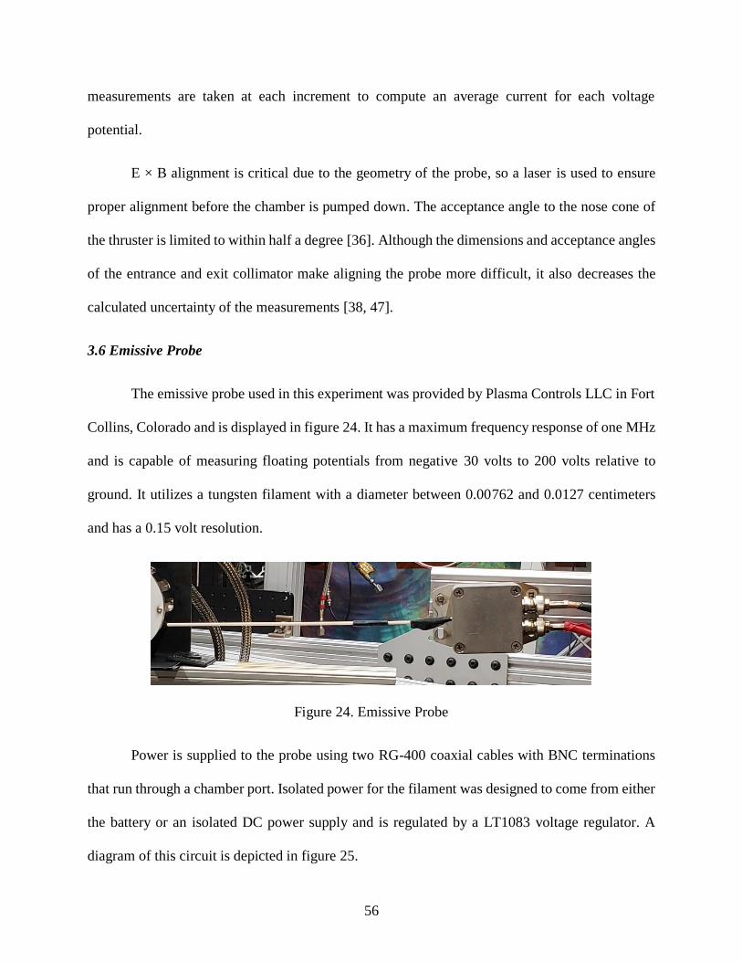
56

measurements are taken at each increment to compute an average current for each voltage

potential.

E × B alignment is critical due to the geometry of the probe, so a laser is used to ensure

proper alignment before the chamber is pumped down. The acceptance angle to the nose cone of

the thruster is limited to within half a degree [36]. Although the dimensions and acceptance angles

of the entrance and exit collimator make aligning the probe more difficult, it also decreases the

calculated uncertainty of the measurements [38, 47].

3.6 Emissive Probe

The emissive probe used in this experiment was provided by Plasma Controls LLC in Fort

Collins, Colorado and is displayed in figure 24. It has a maximum frequency response of one MHz

and is capable of measuring floating potentials from negative 30 volts to 200 volts relative to

ground. It utilizes a tungsten filament with a diameter between 0.00762 and 0.0127 centimeters

and has a 0.15 volt resolution.

Figure 24. Emissive Probe

Power is supplied to the probe using two RG-400 coaxial cables with BNC terminations

that run through a chamber port. Isolated power for the filament was designed to come from either

the battery or an isolated DC power supply and is regulated by a LT1083 voltage regulator. A

diagram of this circuit is depicted in figure 25.

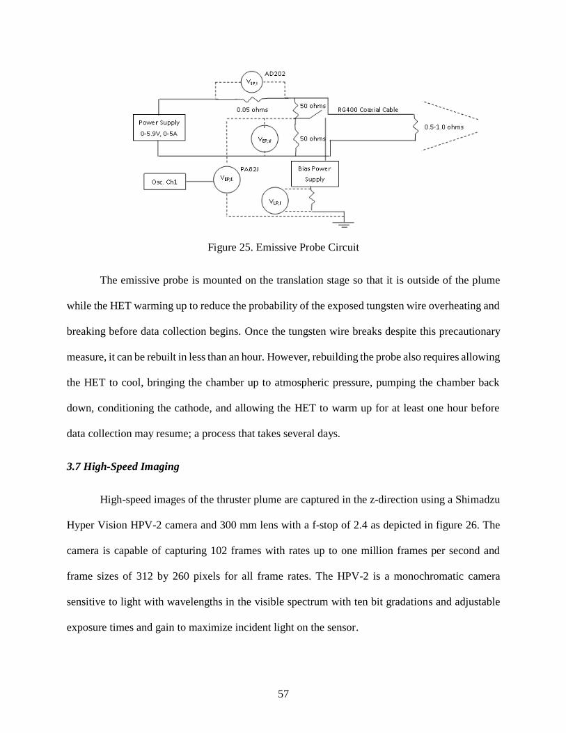
57

Figure 25. Emissive Probe Circuit

The emissive probe is mounted on the translation stage so that it is outside of the plume

while the HET warming up to reduce the probability of the exposed tungsten wire overheating and

breaking before data collection begins. Once the tungsten wire breaks despite this precautionary

measure, it can be rebuilt in less than an hour. However, rebuilding the probe also requires allowing

the HET to cool, bringing the chamber up to atmospheric pressure, pumping the chamber back

down, conditioning the cathode, and allowing the HET to warm up for at least one hour before

data collection may resume; a process that takes several days.

3.7 High-Speed Imaging

High-speed images of the thruster plume are captured in the z-direction using a Shimadzu

Hyper Vision HPV-2 camera and 300 mm lens with a f-stop of 2.4 as depicted in figure 26. The

camera is capable of capturing 102 frames with rates up to one million frames per second and

frame sizes of 312 by 260 pixels for all frame rates. The HPV-2 is a monochromatic camera

sensitive to light with wavelengths in the visible spectrum with ten bit gradations and adjustable

exposure times and gain to maximize incident light on the sensor.

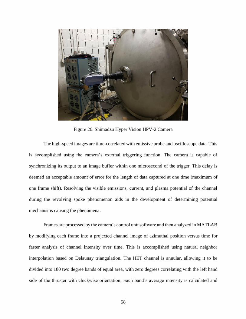
58

Figure 26. Shimadzu Hyper Vision HPV-2 Camera

The high-speed images are time-correlated with emissive probe and oscilloscope data. This

is accomplished using the camera’s external triggering function. The camera is capable of

synchronizing its output to an image buffer within one microsecond of the trigger. This delay is

deemed an acceptable amount of error for the length of data captured at one time (maximum of

one frame shift). Resolving the visible emissions, current, and plasma potential of the channel

during the revolving spoke phenomenon aids in the development of determining potential

mechanisms causing the phenomena.

Frames are processed by the camera’s control unit software and then analyzed in MATLAB

by modifying each frame into a projected channel image of azimuthal position versus time for

faster analysis of channel intensity over time. This is accomplished using natural neighbor

interpolation based on Delaunay triangulation. The HET channel is annular, allowing it to be

divided into 180 two degree bands of equal area, with zero degrees correlating with the left hand

side of the thruster with clockwise orientation. Each band’s average intensity is calculated and

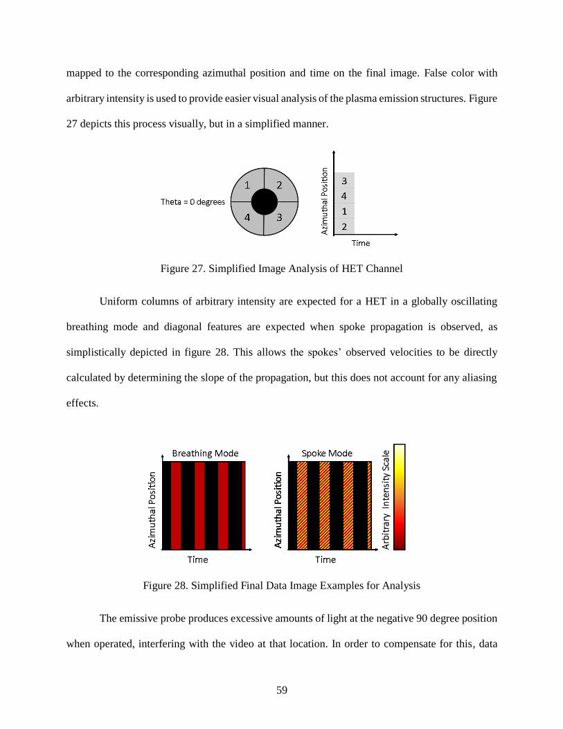
59

mapped to the corresponding azimuthal position and time on the final image. False color with

arbitrary intensity is used to provide easier visual analysis of the plasma emission structures. Figure

27 depicts this process visually, but in a simplified manner.

Figure 27. Simplified Image Analysis of HET Channel

Uniform columns of arbitrary intensity are expected for a HET in a globally oscillating

breathing mode and diagonal features are expected when spoke propagation is observed, as

simplistically depicted in figure 28. This allows the spokes’ observed velocities to be directly

calculated by determining the slope of the propagation, but this does not account for any aliasing

effects.

Figure 28. Simplified Final Data Image Examples for Analysis

The emissive probe produces excessive amounts of light at the negative 90 degree position

when operated, interfering with the video at that location. In order to compensate for this, data

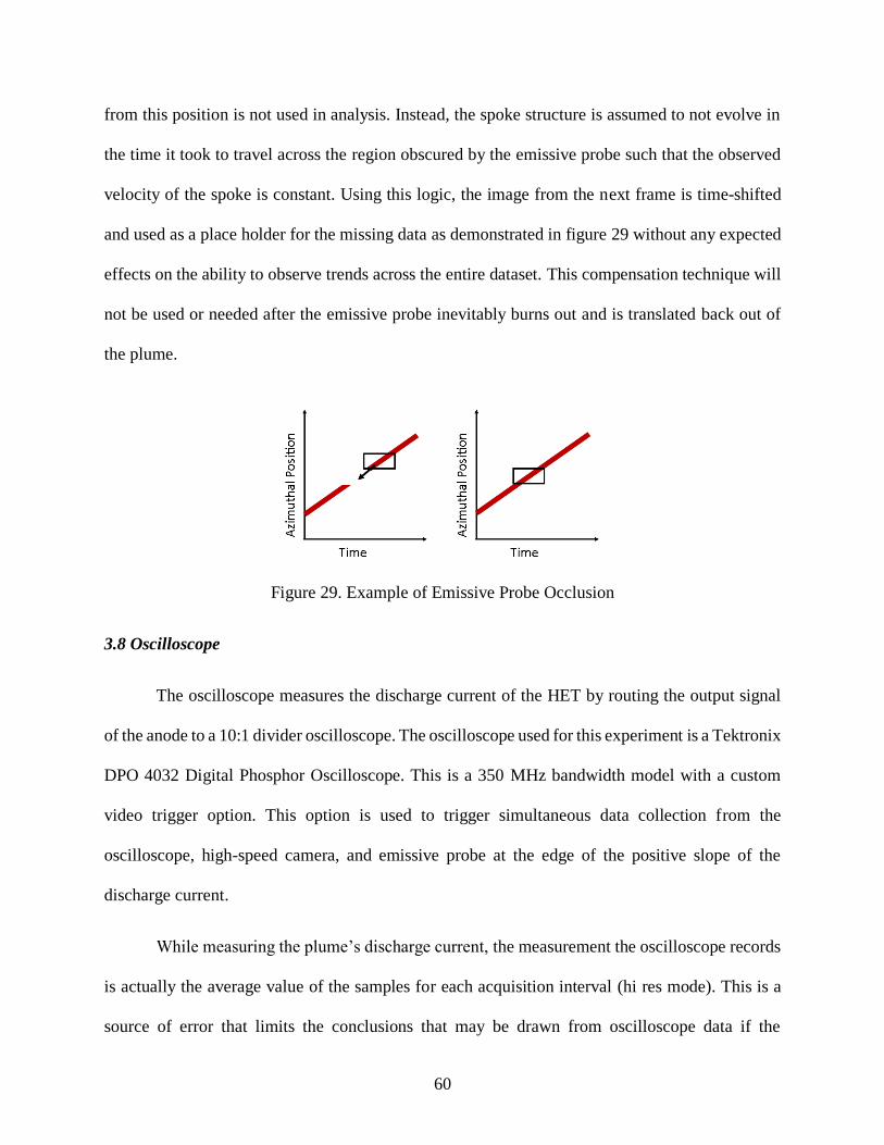
60

from this position is not used in analysis. Instead, the spoke structure is assumed to not evolve in

the time it took to travel across the region obscured by the emissive probe such that the observed

velocity of the spoke is constant. Using this logic, the image from the next frame is time-shifted

and used as a place holder for the missing data as demonstrated in figure 29 without any expected

effects on the ability to observe trends across the entire dataset. This compensation technique will

not be used or needed after the emissive probe inevitably burns out and is translated back out of

the plume.

Figure 29. Example of Emissive Probe Occlusion

3.8 Oscilloscope

The oscilloscope measures the discharge current of the HET by routing the output signal

of the anode to a 10:1 divider oscilloscope. The oscilloscope used for this experiment is a Tektronix

DPO 4032 Digital Phosphor Oscilloscope. This is a 350 MHz bandwidth model with a custom

video trigger option. This option is used to trigger simultaneous data collection from the

oscilloscope, high-speed camera, and emissive probe at the edge of the positive slope of the

discharge current.

While measuring the plume’s discharge current, the measurement the oscilloscope records

is actually the average value of the samples for each acquisition interval (hi res mode). This is a

source of error that limits the conclusions that may be drawn from oscilloscope data if the

61

difference in measured discharge current is too small. However, this data collection method is the

best acquisition mode for this research because other options only retain the first sampled point

from each acquisition interval (sample), only retain the highest and lowest sample contained in

two consecutive acquisition intervals (peak detect), only record the highest and lowest points over

all acquisitions (envelope) or record the average value over several acquisitions instead of just one

(average).

62

IV. Results and Analysis

4.1 Propellant Selection

This experiment was originally intended to be run on krypton gas instead of xenon gas.

This is because chamber plumbing is set up to facilitate both xenon and krypton, and of the two,

krypton is less expensive. However, the switch to xenon was made because the BHT-100-I was

unable to maintain operation for more than thirty minutes using krypton gas. The BHT-100-I most

likely experienced difficulties with krypton but not with xenon because the first ionization energy

of xenon is 1.9 electron volts lower than the first ionization energy of krypton (12.1 eV v. 14 eV).

This increase in the energy required for single ionization may be problematic because of the

permanent magnet under the nose cone, the low discharge power the BHT-100-I operates at,

heating, or a combination of these factors.

The BHT-100-I was able to ignite using krypton gas and experienced the most stable

operation while the mass flow rate of krypton was two times higher than what was expected to be

needed for operation; three times greater required for ignition. Decreasing the mass flow rate any

more than twice the expected amount caused the thruster to immediately stop operating. The HET

would also not ignite until the applied current to the magnet was 1.33 amps. As a comparison, the

HET ignited when the current applied to the magnet was 0.4 amps when using xenon as the

propellant. Also, a solenoid current greater than 1.5 amps should not be applied for an extended

period [23]. The HET is operating with krypton in figure 30 and xenon in figure 31. The additional

source of light in figure 30 is from the window on the other side of the vacuum chamber; this

window was covered in figure 31.

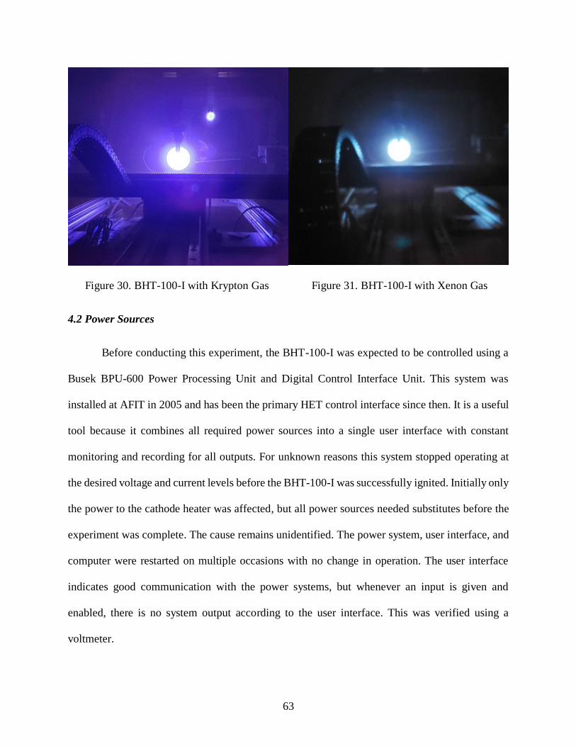
63

Figure 30. BHT-100-I with Krypton Gas Figure 31. BHT-100-I with Xenon Gas

4.2 Power Sources

Before conducting this experiment, the BHT-100-I was expected to be controlled using a

Busek BPU-600 Power Processing Unit and Digital Control Interface Unit. This system was

installed at AFIT in 2005 and has been the primary HET control interface since then. It is a useful

tool because it combines all required power sources into a single user interface with constant

monitoring and recording for all outputs. For unknown reasons this system stopped operating at

the desired voltage and current levels before the BHT-100-I was successfully ignited. Initially only

the power to the cathode heater was affected, but all power sources needed substitutes before the

experiment was complete. The cause remains unidentified. The power system, user interface, and

computer were restarted on multiple occasions with no change in operation. The user interface

indicates good communication with the power systems, but whenever an input is given and

enabled, there is no system output according to the user interface. This was verified using a

voltmeter.

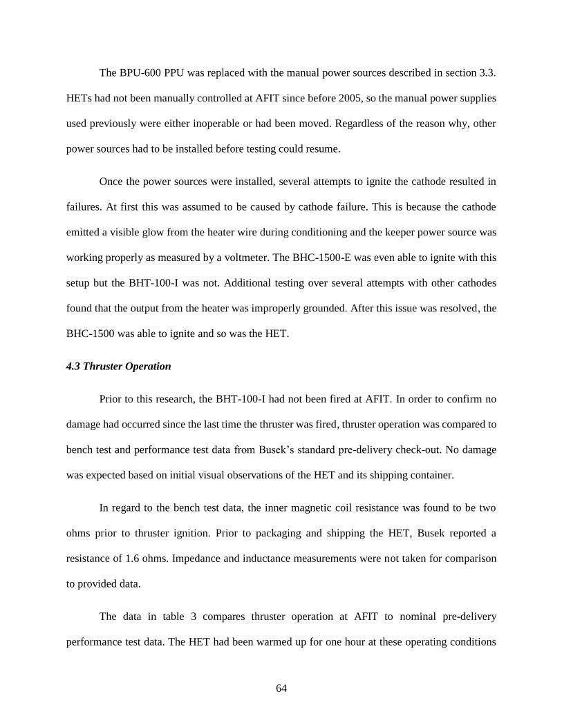
64

The BPU-600 PPU was replaced with the manual power sources described in section 3.3.

HETs had not been manually controlled at AFIT since before 2005, so the manual power supplies

used previously were either inoperable or had been moved. Regardless of the reason why, other

power sources had to be installed before testing could resume.

Once the power sources were installed, several attempts to ignite the cathode resulted in

failures. At first this was assumed to be caused by cathode failure. This is because the cathode

emitted a visible glow from the heater wire during conditioning and the keeper power source was

working properly as measured by a voltmeter. The BHC-1500-E was even able to ignite with this

setup but the BHT-100-I was not. Additional testing over several attempts with other cathodes

found that the output from the heater was improperly grounded. After this issue was resolved, the

BHC-1500 was able to ignite and so was the HET.

4.3 Thruster Operation

Prior to this research, the BHT-100-I had not been fired at AFIT. In order to confirm no

damage had occurred since the last time the thruster was fired, thruster operation was compared to

bench test and performance test data from Busek’s standard pre-delivery check-out. No damage

was expected based on initial visual observations of the HET and its shipping container.

In regard to the bench test data, the inner magnetic coil resistance was found to be two

ohms prior to thruster ignition. Prior to packaging and shipping the HET, Busek reported a

resistance of 1.6 ohms. Impedance and inductance measurements were not taken for comparison

to provided data.

The data in table 3 compares thruster operation at AFIT to nominal pre-delivery

performance test data. The HET had been warmed up for one hour at these operating conditions

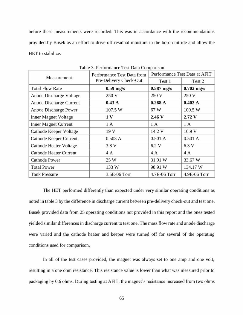
65

before these measurements were recorded. This was in accordance with the recommendations

provided by Busek as an effort to drive off residual moisture in the boron nitride and allow the

HET to stabilize.

Table 3. Performance Test Data Comparison

Measurement Performance Test Data from

Pre-Delivery Check-Out

Performance Test Data at AFIT

Test 1 Test 2

Total Flow Rate 0.59 mg/s 0.587 mg/s 0.702 mg/s

Anode Discharge Voltage 250 V 250 V 250 V

Anode Discharge Current 0.43 A 0.268 A 0.402 A

Anode Discharge Power 107.5 W 67 W 100.5 W

Inner Magnet Voltage 1 V 2.46 V 2.72 V

Inner Magnet Current 1 A 1 A 1 A

Cathode Keeper Voltage 19 V 14.2 V 16.9 V

Cathode Keeper Current 0.503 A 0.501 A 0.501 A

Cathode Heater Voltage 3.8 V 6.2 V 6.3 V

Cathode Heater Current 4 A 4 A 4 A

Cathode Power 25 W 31.91 W 33.67 W

Total Power 133 W 98.91 W 134.17 W

Tank Pressure 3.5E-06 Torr 4.7E-06 Torr 4.9E-06 Torr

The HET performed differently than expected under very similar operating conditions as

noted in table 3 by the difference in discharge current between pre-delivery check-out and test one.

Busek provided data from 25 operating conditions not provided in this report and the ones tested

yielded similar differences in discharge current to test one. The mass flow rate and anode discharge

were varied and the cathode heater and keeper were turned off for several of the operating

conditions used for comparison.

In all of the test cases provided, the magnet was always set to one amp and one volt,

resulting in a one ohm resistance. This resistance value is lower than what was measured prior to

packaging by 0.6 ohms. During testing at AFIT, the magnet’s resistance increased from two ohms

66

to 2.46 ohms after one hour of operation. The magnet’s resistance increased to and stabilized at

2.72 ohms after several hours of operation on multiple testing days. Resistance is expected to

increase with temperature and copper has in increase in resistance of about 0.0039 per Kelvin, so

a 27 degree increase in temperature would explain the observed increase in resistance. The

difference between reported values and measured values indicate a change in the thruster’s

magnetic coil or is the result of a misprint in the provided data measurements.

Additionally, the discharge current was expected to fall within the range of 0.4 to 0.5 amps

with 5 sccm of xenon flowing to the anode, 1 sccm of xenon flowing to the cathode, and a discharge

potential of 250 volts. With 5.05 sccm of xenon flowing to the anode and 1.001 sccm of xenon

flowing to the cathode (first test case at AFIT in table 3) the discharge current was below the

expected range by 0.132 amps. The discharge current met the expected range with a 1.2 sccm

increase in anode mass flow rate.

These results suggest the BHT-100-I operates slightly differently than expected from the

provided check-out data. There were no observations made indicating HET damage so it is possible

that apart from the magnet resistance discrepancy, the difference in thruster operation is due to

mass flow rate calibration errors at AFIT and/or Busek. The BHT-100-I was operated near 10% of

the mass flow rate the system at AFIT was calibrated for and the 1.2 sccm increase required for

nominal discharge current is only 2.4% of the calibrated flow rate.

4.4 Effect of Mass Flow Rate on Discharge Current

The BHT-100-I was designed to operate at power levels between 75 to 125 Watts and the

nominal discharge potential was determined by Busek to fall between the range of 200 to 300

volts. The discharge voltage was varied across this nominal range at several total mass flow rates

67

(cathode mass flow rate held constant at 1.001 sccm) and the discharge current was measured and

recorded in figure 32. The discharge power was calculated and is plotted as a function of discharge

voltage and total mass flow rate in figure 33.

Figure 32. Discharge Voltage v. Current for Different Total Mass Flow Rates

Figure 33. Discharge Voltage v. Power for Different Total Mass Flow Rates

Figures 32 and 33 were used to depict the operating conditions chosen to characterize the

HETs optimal efficiency, divergence angle, and ionization fraction as determined by a Faraday

probe and E × B probe. These points are identified by the larger markers on figures 32 and 33. A

total mass flow rate of 0.702 mg/s was selected because this mass flow rate yielded the expected

discharge current (approximately 0.4 amps) at 250 volts of discharge potential as provided by

Busek, resulting in approximately 100 Watts of discharge power. Additionally, the discharge

power was within the power levels the BHT-100-I was designed to operate at throughout the entire

68

nominal discharge voltage range, allowing the entire range of nominal values to be tested at

constant mass flow rates, magnet current, keeper current, and heater current.

4.5 Thruster Characterization

The experimental setup for phase one from chapter three was used to determine the BHT-

100-I’s performance at various nominal operating conditions using a Faraday probe and E × B

probe. The BHT-100-I’s nominal discharge range is defined by Busek to fall between 200 and 300

volts with corresponding power levels between 75 and 125 Watts [23]. The Faraday probe

measures change in voltages due to ion current and allows the plume’s divergence angle and

current density profile to be calculated when measurements are taken across the plume. The E × B

probe separates ion species by their respective mass and charge so ion species fractions may be

calculated. The HET warmed up for one hour prior to any data collection and ran for thirty minutes

prior to data collection following any user change to the operating parameters.

4.5.1 Equipment Setbacks

As the traverse was conducting radial sweeps with the Faraday probe to measure the current

density of the plume at a discharge voltage of 300 volts, the pressure inside of the vacuum chamber

increased from 5.0E-06 Torr to 7.6E-05 Torr within a few seconds. The RGA showed the increase

in pressure inside the chamber was due to water and nitrogen. The traverse and its cooling system

were immediately powered down and the pressure stopped rapidly ascending shortly after. Based

on this effect, the increase in pressure is assumed to be the result of a coolant leak inside of the

chamber. Nothing unusual was observed prior to the sudden increase in pressure within the

chamber and there were no visible changes detected from outside the chamber to the traverse,

probe, cathode, or HET after the increase in pressure was detected.

69

The traverse is not able to run without the cooling system, so data collection ceased. The

increase in pressure alone was not enough to damage the thruster, but the water inside of the

chamber was concerning. At low pressure any water inside the chamber would quickly vaporize

and would have the potential to damage the HET or cathode. The HET was powered down and the

cryopumps were left on until the HET and cathode had cooled. The HET was removed from the

chamber and the traverse’s cooling system was turned on to check for visible leaks. After running

for approximately thirty minutes, a water droplet was found on one of the cooling system’s

connections on the axial translation stage of the traverse as highlighted in figure 34.

Figure 34. Water Leak from Traverse Cooling System Inside Chamber

The connection at this point was loose and there were no visible cracks or signs of wear on

the plastic tubing. The connection was properly secured, all others were checked and tightened,

and no other leaks were found. Assuming the problem was resolved and testing could resume, the

HET was reinstalled and the chamber was pumped down. Figure 35 shows the RGA interface after

the thruster was operating just prior to powering on the traverse and cooling system.

70

Figure 35. RGA Output during HET Operation

The total pressure inside the chamber during HET operation was 3.98E-06 Torr. Figure 36

shows the RGA output of the pressure inside the chamber immediately after the traverse and

cooling system were turned on.

Figure 36. RGA Output during HET and Traverse Operation

71

The pressure inside the chamber increased to 2.16E-05 Torr in figure 36. This indicates

there was still a cooling leak inside of the vacuum chamber. This leak has not been found and

resolved, presently preventing the traverse from further operation at vacuum pressure. For this

reason, current density measurements were only obtained at the first four operating conditions

labeled in figure 32 since the 300 volt probe sweep was not completed.

Additionally, radial sweeps with the E × B probe could not be safely conducted due to the

leak. Data collection was attempted 40 cm from the thruster’s face in the center of the plume. This

method would not allow species concentrations and ionization regions to be calculated for the

entire plume or allow observation of charge exchange in the wings with increased clarity.

However, it would provide some information about ion species concentrations and ionization

regions directly in front of the thruster. However, after two failed attempts, realigning the probe,

rechecking all wiring and power supplies, increasing the range of bias plate voltages tested,

decreasing the increment between bias voltages, and visually inspecting the interior of the probe

casing for damage, only zeros were measured. The E × B probe’s last recorded use was in 2012.

No issues with the probe were mentioned in the report and xenon was the propellant used [24].

The 40 centimeter radial distance the probe was placed at is not expected to be problematic because

the Faraday probe was able to collect data at this distance and at greater distances without issue.

4.5.2 Current Density Profile

Current density measurements for the entire plume allow an approximate plume

divergence, beam current, and ion production efficiency to be calculated for comparison between

operating conditions. Current density measurements from the first four points labeled on figure 32

were calculated using Faraday probe measurements and equation 47. Based on previous

experiments with the BHT-600 and the BHT-200 [36, 46, 48], higher ion densities are expected

72

directly in front of the ionization regions, at higher discharge voltages, and at smaller radial

distances for the range of values tested. The current density due to charge exchange is expected to

significantly increase at angles greater than 30 degrees to 50 degrees with increasing background

pressure, as observed in other experiments that varied pressure within the chamber [21, 36]. Charge

exchange caused by background pressure and wall scattering are expected to have less drastic

effects on the plume’s current density at smaller angles from the HET centerline.

Figures 37 through 44 display the current density and normalized current density at

different discharge voltages and radial distances as a function of degree from the thruster’s

centerline. Normalized current densities depict the change in current density as a function of angle

from the centerline. These normalized plots allow crossover points, the angles where the

normalized current density begins to deviate with respect to other radial distance measurements,

to be determined. Angles larger than the crossover point angles indicate the wings of the plume.

Figure 37. Faraday Probe Current Density Measurements at 200V

Figure 38. Normalized Faraday Probe Current Density Measurements at 200V

73





74



Figures 37 through 44 depict a decrease in current density at the HET’s centerline. This

dip is due to the annular geometry of the thruster and the distance between the sides of the channel.

This observation confirms the assumption that current density measurements are more accurate if

assumed to be a two-point source instead of a single-point source (section 2.5). This slight decrease

in the current density at the center of the plume is expected to become unobservable as radial

distance is increased because the ratio of the distance between the channels over the radial distance

linearly declines.

At closer radial distances the HET current density profile appears to be skewed to the right.

At a distance of 20 centimeters all operating conditions depict a three degree shift from centerline

and the left side of the profile is similarly skewed to the right. Current density profiles at larger

radial distances are more symmetric. This asymmetric profile is most likely due to experimental

error in determining the HETs exact position within the chamber with respect to the traverse and

75

perfectly aligning the face of the HET to be parallel to the radial axis of the traverse. However,

this may also be the result of slight asymmetries in the HET. Either way, this error is expected to

have less of an effect at greater distances from the HET, matching the observed trend. Unlike

vertical current density measurements taken of the BHT-200 [48], this slight horizontal shift

should not indicate plume distortion due to cathode placement (lower density closer to cathode

orifice) because the cathode is vertically aligned with the HET’s center and the plume was swept

horizontally. However, this cannot be completely ruled out because there may be an asymmetry

due to Hall current circulation effects on the cathode or cathode outflow asymmetry.

The normalized current density plots also indicate a decrease in normalized current density

at the center of the plume between measurements taken at larger radial distances. This is most

likely the effect of neutralization but will be discussed in more detail in section 4.5.6. Using the

right side of the plume, the crossover point is close to 10 degrees at 200 volts, between 10 degrees

and 15 degrees at 225 volts, between 15 degrees and 20 degrees and 250 volts, and between 25

degrees and 35 degrees at 275 volts. Separation of the normalized current densities at the same

discharge voltage between measurements taken at different radial distances continues to increase

after the initial crossover point. This deviation is especially evident on the left side of the plume at

angles greater than 50 degrees and closer distances to the HET. This increase in deviation at the

wings is an expected effect of charge exchange and momentum scattering in the plume. There is

also more variation in the current density at large angles and radial distances, especially on the 200

volt and 275 volt plots. This random variation could be an effect of charge exchange and wall

scattering due to the plume’s close physical proximity to the chamber walls at larger angles and

distances from the HET.

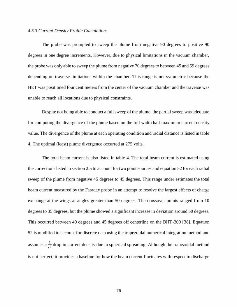
76

4.5.3 Current Density Profile Calculations

The probe was prompted to sweep the plume from negative 90 degrees to positive 90

degrees in one degree increments. However, due to physical limitations in the vacuum chamber,

the probe was only able to sweep the plume from negative 70 degrees to between 45 and 59 degrees

depending on traverse limitations within the chamber. This range is not symmetric because the

HET was positioned four centimeters from the center of the vacuum chamber and the traverse was

unable to reach all locations due to physical constraints.

Despite not being able to conduct a full sweep of the plume, the partial sweep was adequate

for computing the divergence of the plume based on the full width half maximum current density

value. The divergence of the plume at each operating condition and radial distance is listed in table

4. The optimal (least) plume divergence occurred at 275 volts.

The total beam current is also listed in table 4. The total beam current is estimated using

the corrections listed in section 2.5 to account for two point sources and equation 52 for each radial

sweep of the plume from negative 45 degrees to 45 degrees. This range under estimates the total

beam current measured by the Faraday probe in an attempt to resolve the largest effects of charge

exchange at the wings at angles greater than 50 degrees. The crossover points ranged from 10

degrees to 35 degrees, but the plume showed a significant increase in deviation around 50 degrees.

This occurred between 40 degrees and 45 degrees off centerline on the BHT-200 [38]. Equation

52 is modified to account for discrete data using the trapezoidal numerical integration method and

assumes a 1

𝑟2 drop in current density due to spherical spreading. Although the trapezoidal method

is not perfect, it provides a baseline for how the beam current fluctuates with respect to discharge

77

voltage and the beam’s current efficiency (ratio of beam current to discharge current). The optimal

(greatest) beam efficiency occurred at 275 volts.

Table 4. Current Density Profile Calculations

Radial

Distance

(cm)

Discharge

Voltage

(V)

Max Current

Density

(mA/cm2)

Divergence

(°)

Beam

Current

(mA)

Beam

Efficiency

(%)

Discharge

Loss

(W/mA)

20

200 2.657 30.42 219.5 50.23 0.398

225 3.107 27.903 229.4 54.24 0.415

250 3.429 26.85 240.5 58.37 0.428

275 4.103 24.29 265.2 63.66 0.436

30

200 1.142 33.33 226.1 51.74 0.387

225 1.332 30.05 234.6 55.45 0.406

250 1.472 29.40 250.6 60.82 0.411

275 1.69 26.506 268.3 64.43 0.431

40

200 0.6285 34.78 227.8 52.13 0.384

225 0.7302 31.92 235.8 55.75 0.404

250 0.7897 33.80 255.9 62.11 0.403

275 0.909 28.26 267.8 64.29 0.431

50

200 0.3927 35.95 227.9 52.16 0.383

225 0.4532 32.99 234.5 55.44 0.406

250 0.4892 31.51 245.3 59.55 0.420

275 0.5581 29.83 263.8 63.33 0.438

Maximum current density is expected to drop at a rate slightly greater than 1

𝑟2 due to charge

exchange and plume neutralization. At 200 volts the maximum current density is 2.657, 1.142,

0.6285, and 0.3927 mA/cm2. At 225 volts the maximum current density is 3.107, 1.332, 0.7302,

and 0.4532 mA/cm2. The maximum current density at 250 volts is 3.429, 1.472, 0.7897, and 0.4892

mA/cm2. Finally, the maximum current density at 275 volts is 4.103, 1.69, 0.909, and 0.5581

mA/cm2.

78

Divergence is expected to steadily increase due to charge exchange, collisions within the

plume, and background neutrals present in the chamber. At 200 volts the beam divergence is 30.42,

33.33, 34.78, and 35.95 degrees with increasing radial distance. At 225 volts the beam divergence

is 27.903, 30.05, 31.92, and 32.99 degrees. The beam divergence at 250 volts is 26.85, 29.40,

33.80, and 31.51 degrees. Lastly, the divergence at 275 volts is 24.29, 26.506, 28.26, and 29.83

degrees.

The total beam current is expected to vary with respect to radial distance because of charge

exchange, plume neutralization, and wall effects. The beam current at 200 volts is 219.5, 226.1,

227.8, and 227.9 milliamps with a standard deviation of 3.97 milliamps. At 225 volts the total

beam current is 229.4, 234.6, 235.8, and 234.5 milliamps corresponding to a standard deviation of

2.85 milliamps. The total beam current at 250 volts is 240.5, 250.6, 255.9, and 245.3 milliamps.

This corresponds to a standard deviation of 6.65 milliamps. Finally, at 275 degrees the total beam

current is 265.2, 268.3, 267.8, and 263.8 milliamps with a corresponding 2.14 milliamp standard

deviation.

At 200 volts, the beam efficiency has a range of 50.23% to 52.16% with a 0.91% standard

deviation. The beam efficiency at 225 volts is between 54.24% and 55.75% and has a standard

deviation of 0.69%. At 250 volts the beam efficiency is between 58.37% and 62.11% with a

standard deviation of 1.61%. Lastly, the beam efficiency at 275 volts is between 63.33% and

64.43% with a standard deviation of 0.52%.

The discharge loss at 200 volts is 398, 387, 384, and 383 W/A with a standard deviation of

6.88 W/A. At 225 volts the discharge loss is 415, 406, 404, and 406 W/A and the standard deviation

is 4.92 W/A. The discharge loss at 250 volts is 428, 411, 403, and 420 W/A with a 10.85 W/A

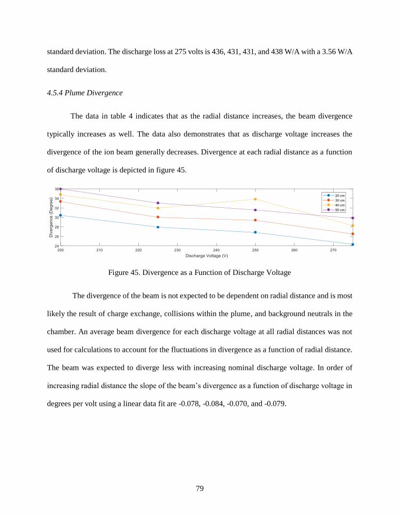
79

standard deviation. The discharge loss at 275 volts is 436, 431, 431, and 438 W/A with a 3.56 W/A

standard deviation.

4.5.4 Plume Divergence

The data in table 4 indicates that as the radial distance increases, the beam divergence

typically increases as well. The data also demonstrates that as discharge voltage increases the

divergence of the ion beam generally decreases. Divergence at each radial distance as a function

of discharge voltage is depicted in figure 45.

Figure 45. Divergence as a Function of Discharge Voltage

The divergence of the beam is not expected to be dependent on radial distance and is most

likely the result of charge exchange, collisions within the plume, and background neutrals in the

chamber. An average beam divergence for each discharge voltage at all radial distances was not

used for calculations to account for the fluctuations in divergence as a function of radial distance.

The beam was expected to diverge less with increasing nominal discharge voltage. In order of

increasing radial distance the slope of the beam’s divergence as a function of discharge voltage in

degrees per volt using a linear data fit are -0.078, -0.084, -0.070, and -0.079.

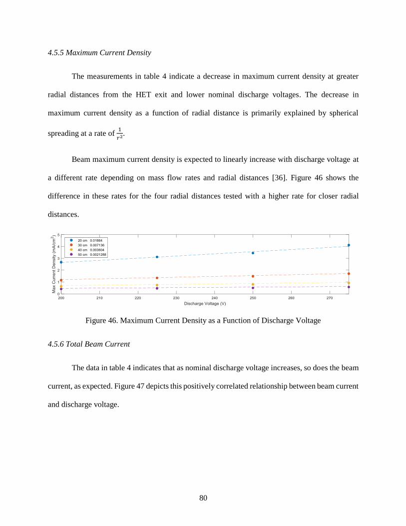
80

4.5.5 Maximum Current Density

The measurements in table 4 indicate a decrease in maximum current density at greater

radial distances from the HET exit and lower nominal discharge voltages. The decrease in

maximum current density as a function of radial distance is primarily explained by spherical

spreading at a rate of 1

𝑟2.

Beam maximum current density is expected to linearly increase with discharge voltage at

a different rate depending on mass flow rates and radial distances [36]. Figure 46 shows the

difference in these rates for the four radial distances tested with a higher rate for closer radial

distances.

Figure 46. Maximum Current Density as a Function of Discharge Voltage

4.5.6 Total Beam Current

The data in table 4 indicates that as nominal discharge voltage increases, so does the beam

current, as expected. Figure 47 depicts this positively correlated relationship between beam current

and discharge voltage.

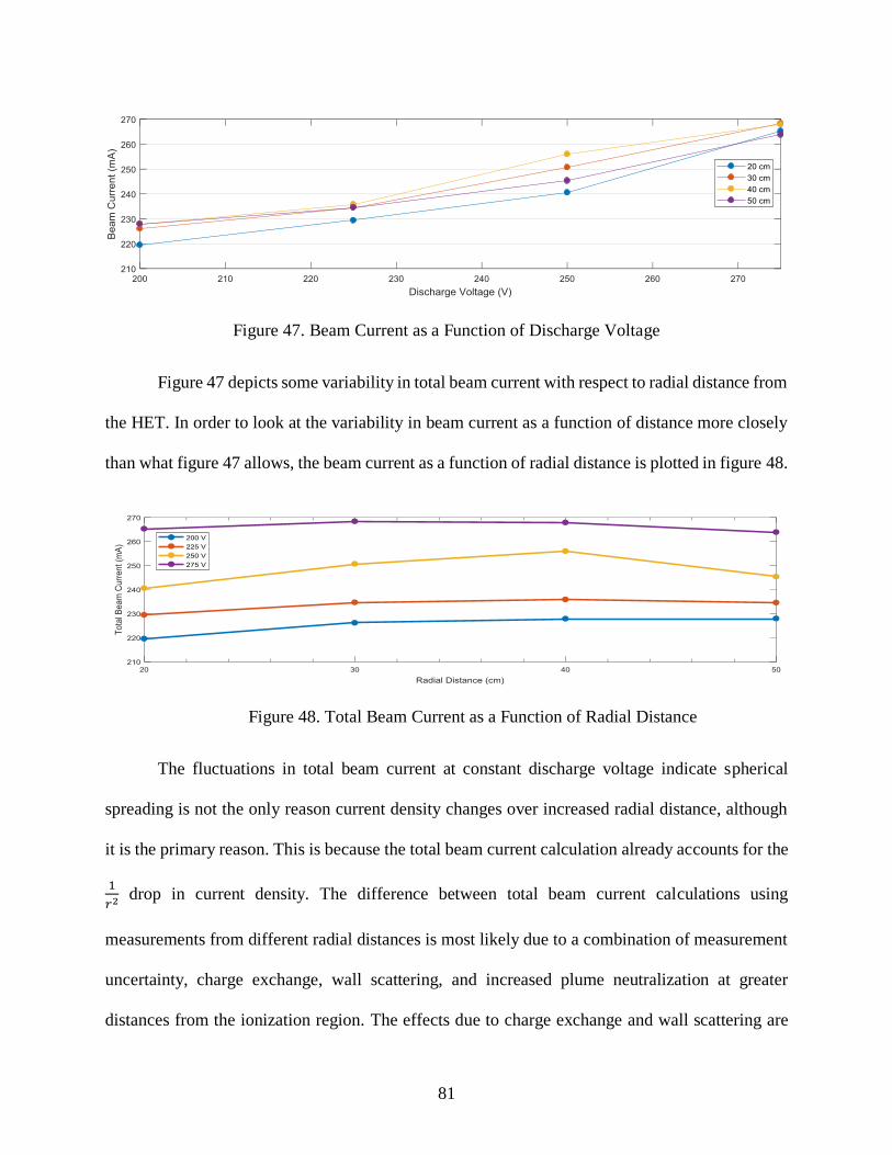
81

Figure 47. Beam Current as a Function of Discharge Voltage

Figure 47 depicts some variability in total beam current with respect to radial distance from

the HET. In order to look at the variability in beam current as a function of distance more closely

than what figure 47 allows, the beam current as a function of radial distance is plotted in figure 48.

Figure 48. Total Beam Current as a Function of Radial Distance

The fluctuations in total beam current at constant discharge voltage indicate spherical

spreading is not the only reason current density changes over increased radial distance, although

it is the primary reason. This is because the total beam current calculation already accounts for the

1

𝑟2 drop in current density. The difference between total beam current calculations using

measurements from different radial distances is most likely due to a combination of measurement

uncertainty, charge exchange, wall scattering, and increased plume neutralization at greater

distances from the ionization region. The effects due to charge exchange and wall scattering are

82

limited in figure 48 because the beam current density was not integrated over angles greater than

45 degrees from the HET’s centerline. Nevertheless, the effects of charge exchange and wall

scattering are not to be disregarded within this range and are still expected to have larger effects

at greater radial distances. Measurement uncertainty is expected to have the greatest effect at closer

radial distances because of potential limitations with the traverse’s ability to match desired angles

at close distances (smaller step size) and greater effects due to misalignment.

4.5.7 Ion Production Efficiency

In order to better quantify the cost of producing ions, the ion production efficiency term,

also known as discharge loss was calculated. This term is a ratio of the power required to produce

ions (discharge power) over the current produced by the ions (beam current) [2]. The relationship

between discharge current and ion production efficiency is depicted in figure 49.

Figure 49. Ion Production Efficiency as a Function of Discharge Voltage

Unlike most efficiency terms, a low ion production efficiency is optimal because it

represents less power loss [2]. There is uncertainty in this calculation because it assumes only

singly-ionized particles are present. There is an average increase in discharge loss as discharge

voltage is increased. The optimal (lowest) discharge loss occurs at 200 volts, although there is a

partial decrease detected between 225 and 250 volts.

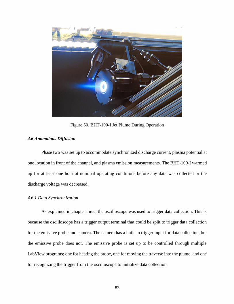
83

Figure 50. BHT-100-I Jet Plume During Operation

4.6 Anomalous Diffusion

Phase two was set up to accommodate synchronized discharge current, plasma potential at

one location in front of the channel, and plasma emission measurements. The BHT-100-I warmed

up for at least one hour at nominal operating conditions before any data was collected or the

discharge voltage was decreased.

4.6.1 Data Synchronization

As explained in chapter three, the oscilloscope was used to trigger data collection. This is

because the oscilloscope has a trigger output terminal that could be split to trigger data collection

for the emissive probe and camera. The camera has a built-in trigger input for data collection, but

the emissive probe does not. The emissive probe is set up to be controlled through multiple

LabView programs; one for heating the probe, one for moving the traverse into the plume, and one

for recognizing the trigger from the oscilloscope to initialize data collection.

84

For undetermined reasons, the computer used to run the LabView programs recognized the

oscilloscope but the LabView program itself did not. This allowed the emissive probe to be heated

and moved into the plume, but data collection was not triggered before the probe burned out. This

interface was not verified for operation before testing because the program required current to be

delivered to the emissive probe and there were no other communication interface errors between

the computer and the oscilloscope.

Before collecting data, the high-speed camera was axially aligned with the HET and

manually focused on the channel. A screenshot of the live camera feed is shown in figure 51.

Figure 51. Screenshot of High-Speed Camera Live Video Feed

Camera settings were set to minimum gain and maximum exposure time for the live feed

in figure 51. The live feed at maximum gain and exposure resulted in a larger, completely white

circle for the HET with no visible difference between the channel and nose cone regions. The

channel diameter was 240 pixels and the cathode orifice was visible at these settings. During data

collection the gain and exposure times were maximized when applicable in order for the camera

to detect as much light as possible. Videos are recorded using the camera’s dedicated 10-bit format

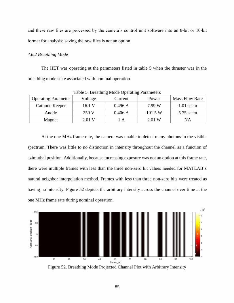
85

and these raw files are processed by the camera’s control unit software into an 8-bit or 16-bit

format for analysis; saving the raw files is not an option.

4.6.2 Breathing Mode

The HET was operating at the parameters listed in table 5 when the thruster was in the

breathing mode state associated with nominal operation.

Table 5. Breathing Mode Operating Parameters

Operating Parameter Voltage Current Power Mass Flow Rate

Cathode Keeper 16.1 V 0.496 A 7.99 W 1.01 sccm

Anode 250 V 0.406 A 101.5 W 5.75 sccm

Magnet 2.01 V 1 A 2.01 W NA

At the one MHz frame rate, the camera was unable to detect many photons in the visible

spectrum. There was little to no distinction in intensity throughout the channel as a function of

azimuthal position. Additionally, because increasing exposure was not an option at this frame rate,

there were multiple frames with less than the three non-zero bit values needed for MATLAB’s

natural neighbor interpolation method. Frames with less than three non-zero bits were treated as

having no intensity. Figure 52 depicts the arbitrary intensity across the channel over time at the

one MHz frame rate during nominal operation.

Figure 52. Breathing Mode Projected Channel Plot with Arbitrary Intensity

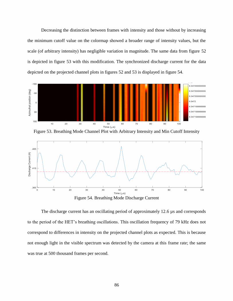
86

Decreasing the distinction between frames with intensity and those without by increasing

the minimum cutoff value on the colormap showed a broader range of intensity values, but the

scale (of arbitrary intensity) has negligible variation in magnitude. The same data from figure 52

is depicted in figure 53 with this modification. The synchronized discharge current for the data

depicted on the projected channel plots in figures 52 and 53 is displayed in figure 54.

Figure 53. Breathing Mode Channel Plot with Arbitrary Intensity and Min Cutoff Intensity

Figure 54. Breathing Mode Discharge Current

The discharge current has an oscillating period of approximately 12.6 µs and corresponds

to the period of the HET’s breathing oscillations. This oscillation frequency of 79 kHz does not

correspond to differences in intensity on the projected channel plots as expected. This is because

not enough light in the visible spectrum was detected by the camera at this frame rate; the same

was true at 500 thousand frames per second.

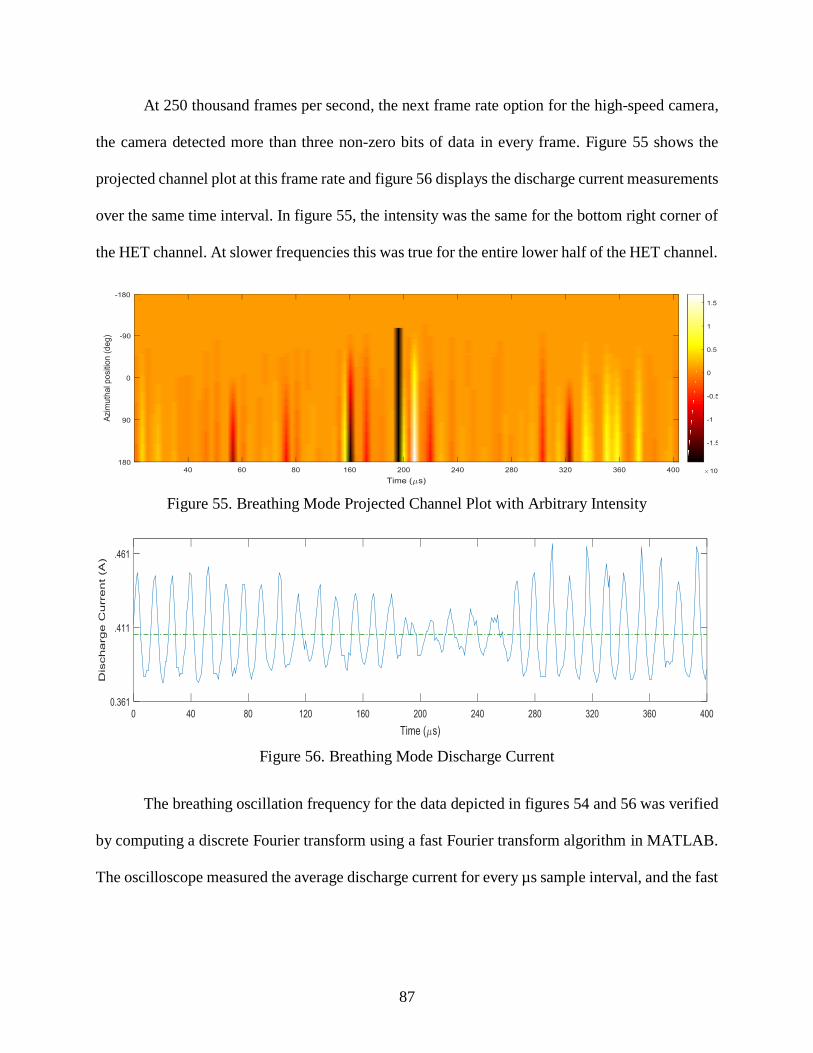
87

At 250 thousand frames per second, the next frame rate option for the high-speed camera,

the camera detected more than three non-zero bits of data in every frame. Figure 55 shows the

projected channel plot at this frame rate and figure 56 displays the discharge current measurements

over the same time interval. In figure 55, the intensity was the same for the bottom right corner of

the HET channel. At slower frequencies this was true for the entire lower half of the HET channel.

Figure 55. Breathing Mode Projected Channel Plot with Arbitrary Intensity

Figure 56. Breathing Mode Discharge Current

The breathing oscillation frequency for the data depicted in figures 54 and 56 was verified

by computing a discrete Fourier transform using a fast Fourier transform algorithm in MATLAB.

The oscilloscope measured the average discharge current for every µs sample interval, and the fast

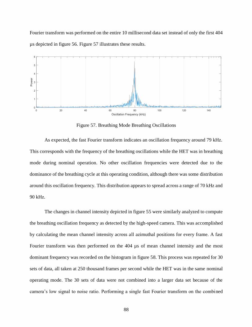
88

Fourier transform was performed on the entire 10 millisecond data set instead of only the first 404

µs depicted in figure 56. Figure 57 illustrates these results.

Figure 57. Breathing Mode Breathing Oscillations

As expected, the fast Fourier transform indicates an oscillation frequency around 79 kHz.

This corresponds with the frequency of the breathing oscillations while the HET was in breathing

mode during nominal operation. No other oscillation frequencies were detected due to the

dominance of the breathing cycle at this operating condition, although there was some distribution

around this oscillation frequency. This distribution appears to spread across a range of 70 kHz and

90 kHz.

The changes in channel intensity depicted in figure 55 were similarly analyzed to compute

the breathing oscillation frequency as detected by the high-speed camera. This was accomplished

by calculating the mean channel intensity across all azimuthal positions for every frame. A fast

Fourier transform was then performed on the 404 µs of mean channel intensity and the most

dominant frequency was recorded on the histogram in figure 58. This process was repeated for 30

sets of data, all taken at 250 thousand frames per second while the HET was in the same nominal

operating mode. The 30 sets of data were not combined into a larger data set because of the

camera’s low signal to noise ratio. Performing a single fast Fourier transform on the combined

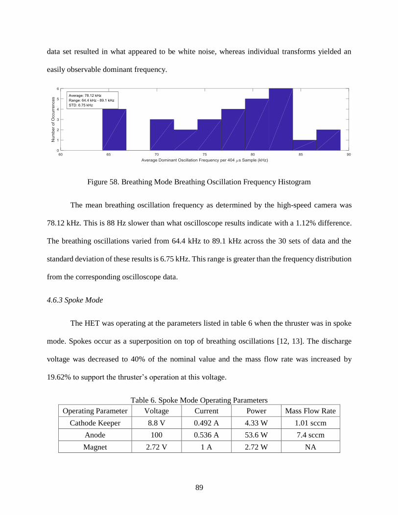
89

data set resulted in what appeared to be white noise, whereas individual transforms yielded an

easily observable dominant frequency.

Figure 58. Breathing Mode Breathing Oscillation Frequency Histogram

The mean breathing oscillation frequency as determined by the high-speed camera was

78.12 kHz. This is 88 Hz slower than what oscilloscope results indicate with a 1.12% difference.

The breathing oscillations varied from 64.4 kHz to 89.1 kHz across the 30 sets of data and the

standard deviation of these results is 6.75 kHz. This range is greater than the frequency distribution

from the corresponding oscilloscope data.

4.6.3 Spoke Mode

The HET was operating at the parameters listed in table 6 when the thruster was in spoke

mode. Spokes occur as a superposition on top of breathing oscillations [12, 13]. The discharge

voltage was decreased to 40% of the nominal value and the mass flow rate was increased by

19.62% to support the thruster’s operation at this voltage.

Table 6. Spoke Mode Operating Parameters

Operating Parameter Voltage Current Power Mass Flow Rate

Cathode Keeper 8.8 V 0.492 A 4.33 W 1.01 sccm

Anode 100 0.536 A 53.6 W 7.4 sccm

Magnet 2.72 V 1 A 2.72 W NA

90

Similar to breathing mode results, the camera was unable to detect an adequate number of

photons in the visible spectrum at one MHz frame rates or 500 thousand frames per second. There

was also not enough light detected at 250 thousand frames per second to observe spokes or spoke

propagation. This is probably due to the 52.81% decrease in anode power, where fewer collisions,

and therefore photons in the visible spectrum, are expected despite an increase in mass flow rate.

Figure 59 depicts the projected channel plot with arbitrary intensity at 250 thousand frames per

second.

Figure 59. Spoke Mode Projected Channel Plot with Arbitrary Intensity and Min Cutoff

At 125 thousand frames per second the camera detected more than three non-zero bits in

every frame, but no rotating spokes were detected in 30 separate 808 µs data samples. There were

also no rotating spokes detected for data samples collected at 63 thousand frames per second. At

slower frame rates, the rotating spokes are not expected to be visible because nearly constant

intensity was observed and the rotating spokes are expected to oscillate at a faster frequency than

the breathing oscillations.

Observing no spokes, or azimuthal increases in intensity within the channel, at a lower

discharge power is not surprising after detecting such little variation in intensity for breathing

oscillations at the same sampling rate during nominal operation. This is not to say the spokes were

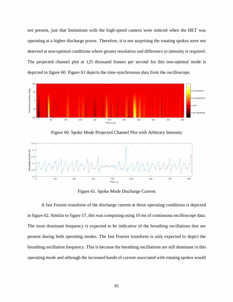
91

not present, just that limitations with the high-speed camera were noticed when the HET was

operating at a higher discharge power. Therefore, it is not surprising the rotating spokes were not

detected at non-optimal conditions where greater resolution and difference in intensity is required.

The projected channel plot at 125 thousand frames per second for this non-optimal mode is

depicted in figure 60. Figure 61 depicts the time-synchronous data from the oscilloscope.

Figure 60. Spoke Mode Projected Channel Plot with Arbitrary Intensity

Figure 61. Spoke Mode Discharge Current

A fast Fourier transform of the discharge current at these operating conditions is depicted

in figure 62. Similar to figure 57, this was computing using 10 ms of continuous oscilloscope data.

The most dominant frequency is expected to be indicative of the breathing oscillations that are

present during both operating modes. The fast Fourier transform is only expected to depict the

breathing oscillation frequency. This is because the breathing oscillations are still dominant in this

operating mode and although the increased bands of current associated with rotating spokes would

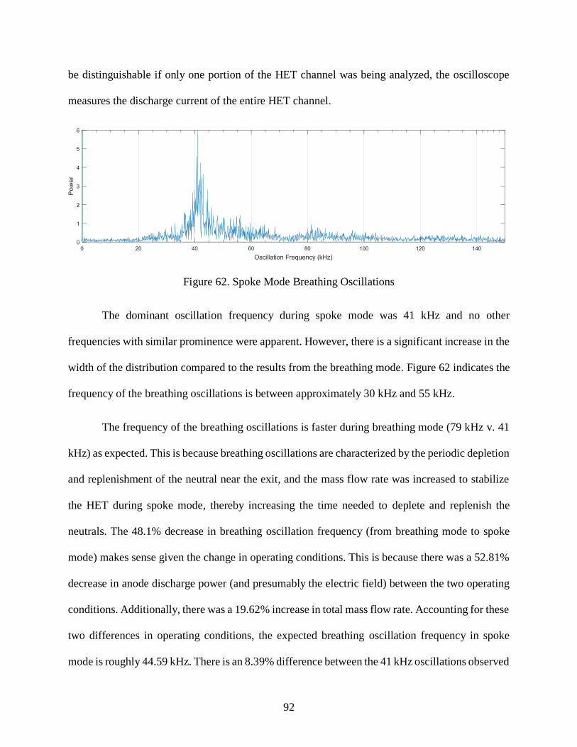
92

be distinguishable if only one portion of the HET channel was being analyzed, the oscilloscope

measures the discharge current of the entire HET channel.

Figure 62. Spoke Mode Breathing Oscillations

The dominant oscillation frequency during spoke mode was 41 kHz and no other

frequencies with similar prominence were apparent. However, there is a significant increase in the

width of the distribution compared to the results from the breathing mode. Figure 62 indicates the

frequency of the breathing oscillations is between approximately 30 kHz and 55 kHz.

The frequency of the breathing oscillations is faster during breathing mode (79 kHz v. 41

kHz) as expected. This is because breathing oscillations are characterized by the periodic depletion

and replenishment of the neutral near the exit, and the mass flow rate was increased to stabilize

the HET during spoke mode, thereby increasing the time needed to deplete and replenish the

neutrals. The 48.1% decrease in breathing oscillation frequency (from breathing mode to spoke

mode) makes sense given the change in operating conditions. This is because there was a 52.81%

decrease in anode discharge power (and presumably the electric field) between the two operating

conditions. Additionally, there was a 19.62% increase in total mass flow rate. Accounting for these

two differences in operating conditions, the expected breathing oscillation frequency in spoke

mode is roughly 44.59 kHz. There is an 8.39% difference between the 41 kHz oscillations observed

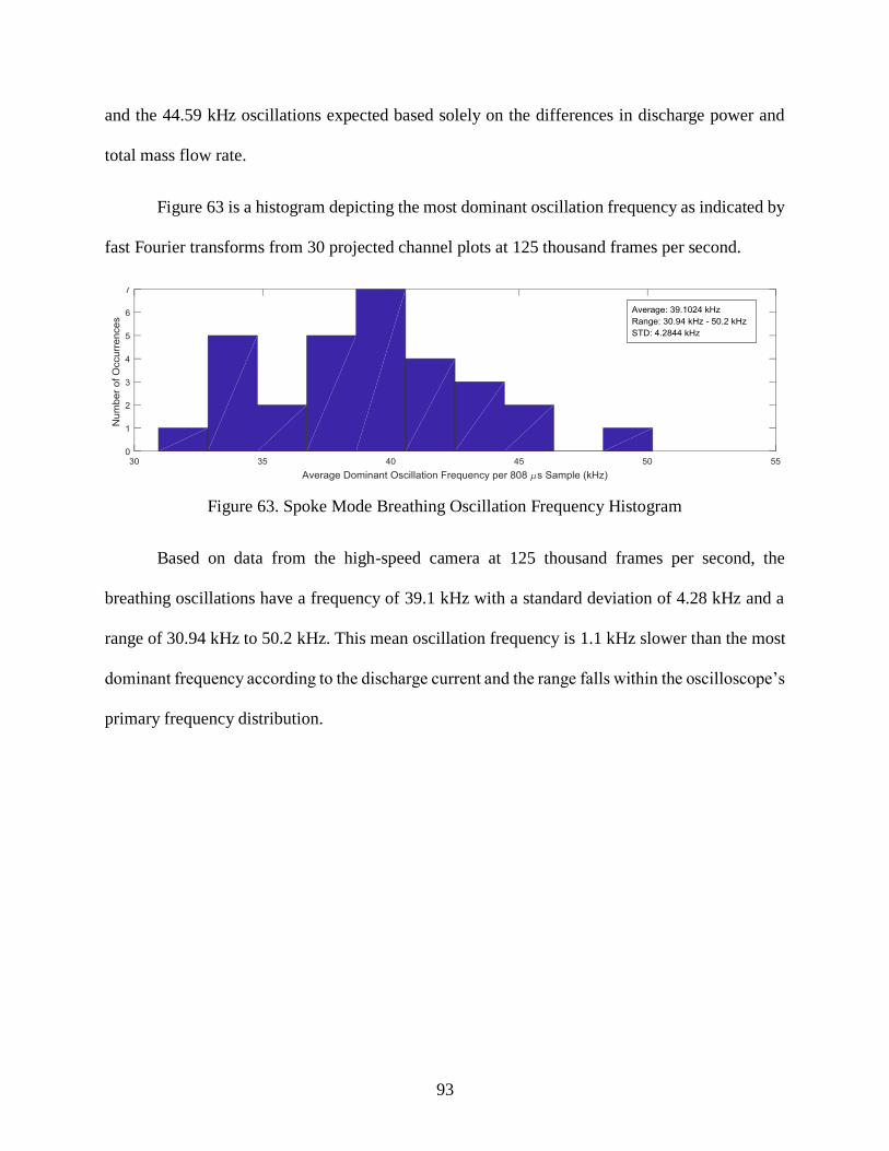
93

and the 44.59 kHz oscillations expected based solely on the differences in discharge power and

total mass flow rate.

Figure 63 is a histogram depicting the most dominant oscillation frequency as indicated by

fast Fourier transforms from 30 projected channel plots at 125 thousand frames per second.

Figure 63. Spoke Mode Breathing Oscillation Frequency Histogram

Based on data from the high-speed camera at 125 thousand frames per second, the

breathing oscillations have a frequency of 39.1 kHz with a standard deviation of 4.28 kHz and a

range of 30.94 kHz to 50.2 kHz. This mean oscillation frequency is 1.1 kHz slower than the most

dominant frequency according to the discharge current and the range falls within the oscilloscope’s

primary frequency distribution.

94

V. Conclusions

The BHT-100-I is not a commercially available thruster and it is designed to operate at

lower power levels than Busek’s commercially available HETs. It has a basic HET design with

additional features intended to decrease erosion and thus increase the lifetime of the thruster. These

features include a permanent magnet under the nose cone, boron nitride lining at the exit plane,

and plasma ground screens. It was also manufactured with materials and coatings that are

compatible with iodine.

The original intent of this research was to validate the BHT-100-I operated as expected

using pre-delivery checkout measurements from the manufacturer, to characterize its nominal

performance at various mass flow rates and discharge voltages, and to investigate anomalous

diffusion within the HET’s channel. The HET was projected to be characterized using

measurements of the plume’s current density profile and ion species fractions from a Faraday

probe and E × B probe, respectively. Plasma oscillations, including those associated with

anomalous diffusion, were expected to be observed using time-synchronous plasma potential,

visible emission, and discharge current measurements with an emissive probe, high-speed camera,

and oscilloscope at high sampling rates.

Many challenges with equipment arose as this research was conducted, and not every

challenge was overcome. This limited the scope of the experiment and prohibited some of the

objectives from being fully met, increasing the amount of future work required. Future work is

needed to better understand how the modifications made to the BHT-100-I affect its operation.

This requires additional investigation to determine the source of several equipment issues.

95

5.1 Summary of Results

In order for the HET to meet expected performance parameters, the anode mass flow rate

had to be increased by approximately 1 sccm of xenon. Although this was unexpected, it does not

indicate any damage sustained by the HET and may be explained by a mass flow rate calibration

error.

The Faraday probe was used to sweep the plume at four radial distances for four nominal

discharge voltages. The measured increase in voltage was used to establish a current density profile

of the plume. Using the current density profile from negative 45 degrees to 45 degrees from the

HET’s centerline the beam’s divergence, beam current, and discharge loss were calculated at each

operating condition and radial distance. Using this information, the overall optimal discharge

voltage for the operating conditions tested is between 225 and 250 volts, corresponding to a

discharge power range of 95 to 103 Watts.

The oscilloscope was used to observe fluctuations in discharge current while the HET was

operating in breathing mode and spoke mode. The frequency of the breathing oscillations

decreased when the mass flow rate to the HET was increased and the discharge current increased

when the discharge voltage decreased. There was also a larger frequency distribution associated

with discharge current oscillations while the HET was in spoke mode.

The high-speed camera was unable to detect any azimuthal bands of increased intensity

(spokes) while the HET was in spoke mode. At one Mfps and 500 kfps the camera was not sensitive

enough to adequately capture the effects of the HET’s breathing oscillations. The camera was

sensitive enough to detect breathing oscillations at 250 kfps during breathing mode operation, but

not while the HET was in spoke mode due to the decrease in discharge power. Breathing

96

oscillations were observable at 125 kfps while the HET was in spoke mode. High-speed

phenomenon was not observable at lower frame rates.

5.2 Next Steps

The largest issue that needs to be resolved before the BHT-100-I can be further evaluated

is the coolant leak inside of the chamber. Traverse operation is required to radially sweep the

plume with sensors and to translate sensors into the plume when needed. All leaks need to be found

and fixed before the traverse can be operated at vacuum pressure without causing potential damage

to the thruster and cathode.

The BPU-600 PPU should also be investigated further. HETs can be manually operated,

but the PPU provides a convenient interface for controlling, monitoring, and recording all

operating parameters, excluding mass flow rates. The reason the PPU stopped working is still

unclear.

Lastly, the E × B probe requires further attention. There are no visible defects inside the

probe’s external casing, but the probe is most likely damaged. Power supplies and electrical

connections to the probe were verified multiple times and the probe has not been used to collect

data for several years. There could be an issue with the permanent magnets, voltage plates, or there

may be erosion within the probe. Any type of obstruction within the collimator or drift tube would

also affect data collection and is a possibility based on how the probe was stored since its last

recorded use.

5.3 Future Work

Four operating conditions were used to characterize the HET’s plume properties. Although

this is a good start, the thruster can operate at a much wider variety of conditions not examined in

97

this research. This research focused only on the effects of varying the discharge voltage on the

plume, but mass flow rates and magnet current can be varied as well. This means that the BHT-

100-I has multiple operating conditions that result in a discharge power around 100 Watts.

Research was limited to the HET’s nominal operating range because this is where operation is

expected to be most efficient, but its high and low operating boundaries could be tested as well.

Comparing the plume’s properties at additional operating conditions and comparing the results to

data from the BHT-200 (accounting for decreased discharge power) could offer valuable insight

about how the modifications to the BHT-100-I affect plume properties.

The BHT-100-I’s plume could also be measured with additional sensors such as an inverted

pendulum stand to measure thrust and specific impulse or a magnetic sensor to measure the Hall

current. These sensors are already at AFIT and have been used with the BHT-600. However, they

may not be sensitive enough for the BHT-100-I without modification because of the decrease in

thrust and magnetic field fluctuations as compared to the 600 Watt HET.

Ideally, the BHT-100-I could also be run at length to test the claims that the modifications

made extend the life of the HET. Due to the length and nature of the master’s program at AFIT,

this is not feasible. The vacuum chamber is needed for multiple experiments and it takes time for

students to familiarize themselves with HETs before testing could begin.

The BHT-100-I could also be run at other non-optimal operating conditions where the

rotating spokes are expected to be observable. With a higher mass flow rate there may be enough

variation in arbitrary intensity for detection with the high-speed camera and 300 mm lens. A high-

speed camera and lens with a better resolution or a higher maximum frame rate (without decreasing

the number of pixels per frame) could also reveal more information about the rotating spokes and

how these relate to thruster operation. AFIT has a larger lens that would be more sensitive to

98

photon emission in the visible spectrum, but the manual lens is not physically compatible with the

camera. The high-speed camera is only compatible with lenses that can be operated in manual and

auto-focusing modes. If an adapter ring were found, this lens could provide the resolution needed

to detect the rotating spokes on the BHT-100-I. Additionally, there are newer camera models that

have higher maximum frame rates. However, without increased resolution or the ability to observe

photons outside of the visible spectrum, the higher frame rate would not be beneficial.

99

Appendix A – Thruster Operating Procedures

Preparation

1. Secure all required sensors and mounts in chamber.

2. Only handle the cathode and thruster with protective gloves and store cathode and thruster in

a climate-controlled cabinet while not in use.

3. Visually inspect cathode and thruster for damage.

4. Mount cathode to thruster with aluminum mounting plate.

5. Mount thruster in chamber.

6. Connect all wires, ground thruster body, and verify electrical connections.

7. Connect propellant lines to cathode and thruster using new VCR seal fittings and ensure no

torque is applied to the cathode or thruster while attaching lines.

8. Secure both chamber doors.

9. Start pump down procedure and do not proceed until total vacuum chamber pressure is below

10-5 Torr as observed by ExTorr’s RGA Vacuum Plus software.

10. Purge propellant lines of residual air by turning on MKS four-channel read out and opening

flow controllers to anode and cathode as well as propellant regulator valve. Turn on channels

three and four and set to maximum flow. Wait until propellant lines are empty (approximately

30 minutes) and then close flow controllers and valves and turn off MKS four-channel read

out.

Condition Cathode

1. Apply 2 amps of current to cathode heater for a minimum of 90 minutes.

2. Increase cathode heater current to 4 amps for a minimum of 90 minutes.

100

3. Increase cathode heater current to 6 amps for a maximum of 30 minutes. Cathode should begin

to glow hot shortly after increasing current to 6 amps.

Ignite Cathode

1. Begin propellant flow to cathode at 1 sccm (typically enough flow for a reliable ignition) and

ensure propellant increases on RGA.

2. Set cathode heater supply to 6.5 amps for a minimum of four minutes.

3. Set cathode keeper supply to 0.5 amps of current and 600 volts. Cathode has ignited when

keeper current is greater than 0.1 amps and within 3-6 minutes of total heating time.

4. If the cathode does not ignite, turn the keeper power supply off, wait ten minutes, and reattempt

step three. Increasing the mass flow rate and slowly increasing the heater current may help

ignite the cathode. Never exceed 8 amps of current to the heater.

Ignite Thruster

1. Begin propellant flow to thruster at 5 sccm and ensure propellant increases on RGA Vacuum

Plus software. Verify background pressure remains less than 10-5 Torr while operating.

2. Apply 1 amp of current to solenoid.

3. Apply discharge potential of 250 volts or similar to anode to ignite discharge. If the thruster

does not ignite, decrease the current to the solenoid until ignition occurs, and then slowly

increase it.

4. Immediately adjust discharge power supply and magnet power supply so discharge is in

voltage limit and current is near minimum. The discharge current is expected to be around 0.4

amps.

5. Turn off the cathode heater.

101

6. Allow the thruster to stabilize for one hour (preferably longer) before testing to drive off

residual moisture in the boron nitride. This is not required for subsequent testing if vacuum has

not been broken. Ensure chamber pressure remains below 10-5 Torr during operation or thruster

damage may occur.

Secure Thruster

1. Turn off the power to the anode, magnet, and keeper (the heater should already be turned off).

2. Stop propellant flow to the anode and cathode and power off the MKS four-channel readout.

3. Close the propellant bottle valves and regulators into the chamber.

4. Wait for the thruster and cathode to completely cool (at least two hours but preferably until the

next day). Stop vacuum chamber pumping procedure and turn off the RGA Vacuum Plus

software.

5. Start Nitrogen flow into the chamber and release all latches on at least one of the doors.

6. Stop Nitrogen flow into the chamber when atmospheric pressure has been reached (usually

takes 2 hours).

7. Vent the chamber by opening both doors. Wait at least 15 minutes before entering chamber to

ensure an adequate amount of oxygen has made its way into the chamber.

8. Detach wires and propellant lines and place thruster and cathode back in climate-controlled

cabinet.

102

Appendix B – Characterization Operating Procedures

Preparation

1. Install the E × B probe and Faraday probe onto rotating stage such that the probe tips will be

level with the center of the thruster. Use of a laser is recommended for aligning the E × B

probe.

2. Home the translation stage to the (0,0,0) position.

3. Determine the location of the center of the thruster (CR and CZ) with respect to the absolute

coordinates of the stages at r = 0 and z = 0. Center of one of the channels can also be used as

the specified point of rotation if desired.

4. Determine the position of each of the probe tips with respect to the stage position (Lp and α).

This is measured from the probe orifice to the theta axis of rotation and the angle is measured

from the z-axis to the location of the probe.

Figure 64. Beam Mapper Overview Diagram

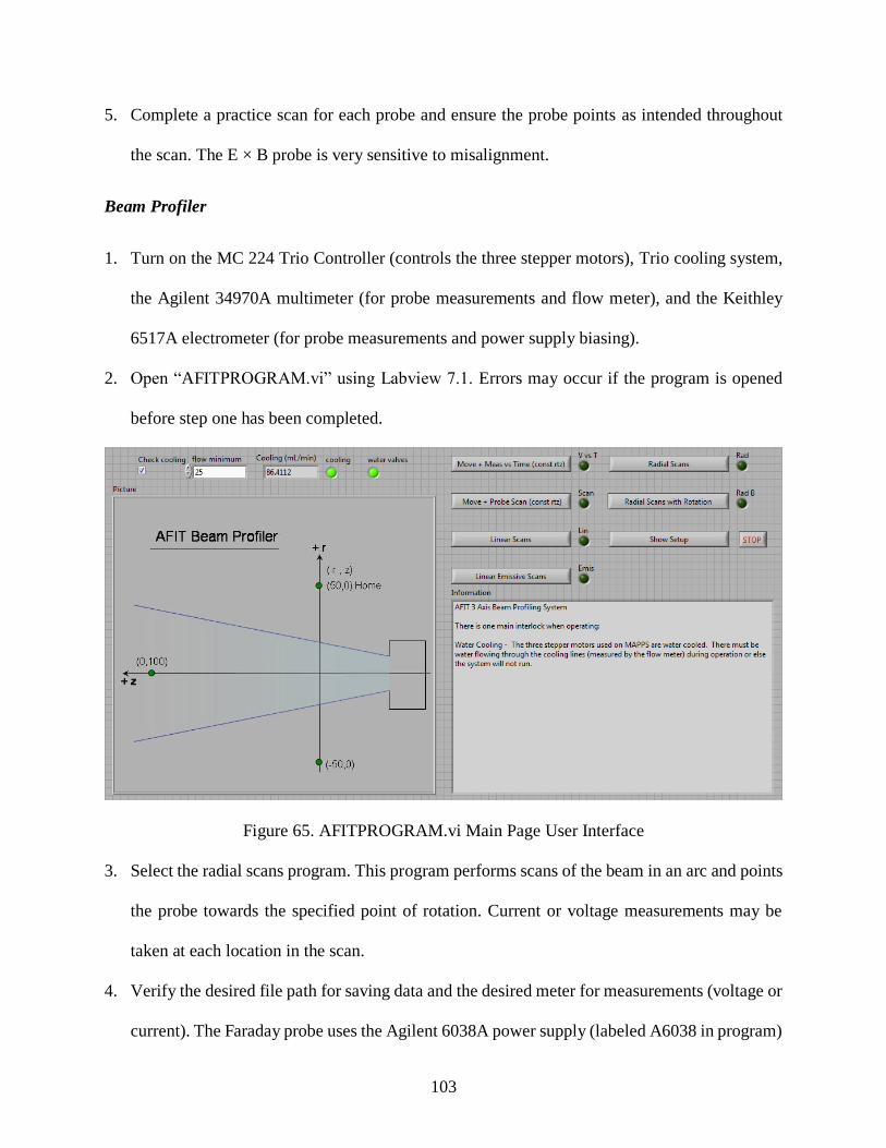
103

5. Complete a practice scan for each probe and ensure the probe points as intended throughout

the scan. The E × B probe is very sensitive to misalignment.

Beam Profiler

1. Turn on the MC 224 Trio Controller (controls the three stepper motors), Trio cooling system,

the Agilent 34970A multimeter (for probe measurements and flow meter), and the Keithley

6517A electrometer (for probe measurements and power supply biasing).

2. Open “AFITPROGRAM.vi” using Labview 7.1. Errors may occur if the program is opened

before step one has been completed.

Figure 65. AFITPROGRAM.vi Main Page User Interface

3. Select the radial scans program. This program performs scans of the beam in an arc and points

the probe towards the specified point of rotation. Current or voltage measurements may be

taken at each location in the scan.

4. Verify the desired file path for saving data and the desired meter for measurements (voltage or

current). The Faraday probe uses the Agilent 6038A power supply (labeled A6038 in program)

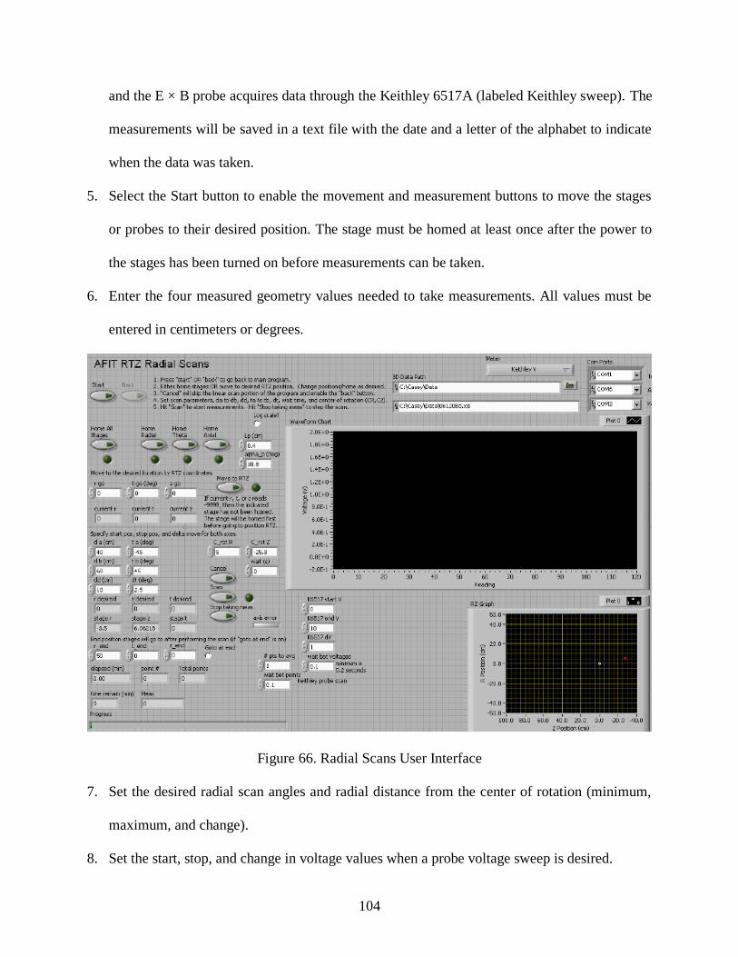
104

and the E × B probe acquires data through the Keithley 6517A (labeled Keithley sweep). The

measurements will be saved in a text file with the date and a letter of the alphabet to indicate

when the data was taken.

5. Select the Start button to enable the movement and measurement buttons to move the stages

or probes to their desired position. The stage must be homed at least once after the power to

the stages has been turned on before measurements can be taken.

6. Enter the four measured geometry values needed to take measurements. All values must be

entered in centimeters or degrees.

Figure 66. Radial Scans User Interface

7. Set the desired radial scan angles and radial distance from the center of rotation (minimum,

maximum, and change).

8. Set the start, stop, and change in voltage values when a probe voltage sweep is desired.

105

9. Push the Scan button to begin the beam scan. The stages should begin moving and the

measurements should appear on the charts. The LED next to the Scan button will illuminate

when the scan is complete. At this point, another scan may be started by pressing the Start

button.

10. The system must be rewired to switch between probes for data collection.

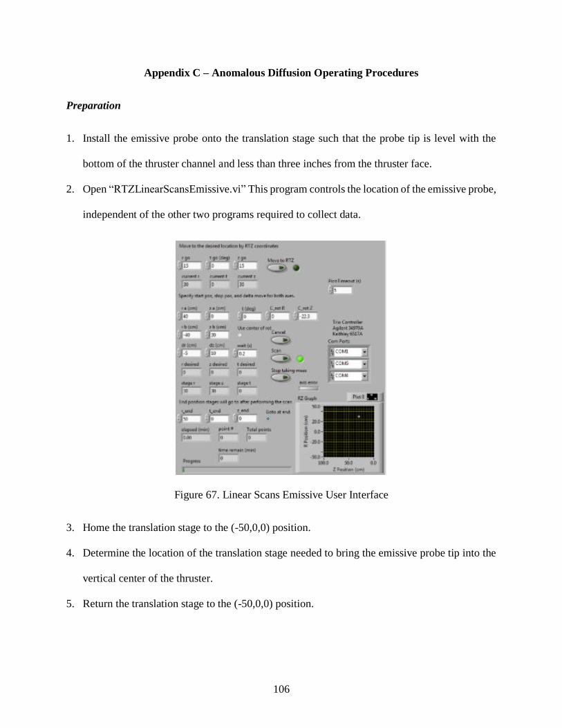
106

Appendix C – Anomalous Diffusion Operating Procedures

Preparation

1. Install the emissive probe onto the translation stage such that the probe tip is level with the

bottom of the thruster channel and less than three inches from the thruster face.

2. Open “RTZLinearScansEmissive.vi” This program controls the location of the emissive probe,

independent of the other two programs required to collect data.

Figure 67. Linear Scans Emissive User Interface

3. Home the translation stage to the (-50,0,0) position.

4. Determine the location of the translation stage needed to bring the emissive probe tip into the

vertical center of the thruster.

5. Return the translation stage to the (-50,0,0) position.

107

6. Synchronize high-speed camera, emissive probe, and oscilloscope using equal length wiring

from the oscilloscope’s trigger signal output to the camera’s internal trigger input and emissive

circuit.

High-Speed Camera

1. Mount lens on camera and setup tripod system in center of chamber window. Ensure the

camera lens is supported.

2. Power on system and manually focus the camera on the HET channel.

3. Change operating parameters to external trigger mode with cooling and desired amount of gain,

exposure time, frame rate, and file type.

Emissive Probe

1. Verify the emissive probe filament is not broken by measuring resistance through BNC fittings

on aluminum housing and replace probe filament if necessary.

2. Open “2014AFITEmisUSB6002GENERATEDIGITAL.vi” using LabView. This program

controls the heating of the emissive filament, independent of the other two programs.

108

Figure 68. Emissive Probe Generate Digital User Interface

3. Set the Fil I setting to level 0 to avoid prematurely burning out the probe’s filament.

4. Select either battery power or external DC power using the Circuit state R2 P0.1 toggle. Charge

the battery if required. If the DC supply is selected, the supply should be between 7.4-9 volts

and floating.

5. Open Labview PicoScope program to monitor the probe’s floating potential.

6. Increase the filament voltage by increasing the Fil I setting level until the filament glows white

hot and starts to emit electrons. 15-16 is the recommended level for 0.005” of tungsten wire

(~3.25 amps of current).

a. Increasing filament emission lets the probe float closer to plasma potential at the

expense of decreased life and increased risk of burnout.

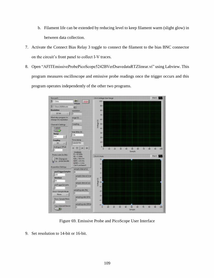
109

b. Filament life can be extended by reducing level to keep filament warm (slight glow) in

between data collection.

7. Activate the Connect Bias Relay 3 toggle to connect the filament to the bias BNC connector

on the circuit’s front panel to collect I-V traces.

8. Open “AFITEmissiveProbePicoScope5242BVerDsavedataRTZlinear.vi” using Labview. This

program measures oscilloscope and emissive probe readings once the trigger occurs and this

program operates independently of the other two programs.

Figure 69. Emissive Probe and PicoScope User Interface

9. Set resolution to 14-bit or 16-bit.

110

10. Select measurement range to be larger than the observed signal. Select AC coupling to

eliminate the DC-offset of the signal and leave only the time-varying portion of the waveform.

11. Scale the probe to match the switch setting on the oscilloscope.

12. Input the desired number of data points to collect and save after the trigger occurs.

13. Set desired location where oscilloscope and emissive probe data should be saved.

Oscilloscope

1. Adjust the vertical position and scale as well as the horizontal position and scale. The

horizontal position determines the number of pre-trigger and post trigger samples. The

horizontal scale determines the size of the acquisition window relative to the waveform.

2. Set the trigger level to the midpoint of the waveform. This may be done manually or by pushing

the “Set to 50%” button.

3. Select the trigger type as edge with increasing slope to set the trigger on a rising edge.

4. Push single to take a single acquisition. Run/Stop should not be used because the oscilloscope

will enter trigger mode almost as soon as the data from the last trigger was collected. The

emissive probe will be able to take time synchronous data with the oscilloscope using this

method, but the high-speed camera will not. This is because the camera requires time between

each data collection to offload the data from the camera to the computer.

111

References

[1] R. G. Jahn, Physics of Electric Propulsion, Mineola: Dover, 2016.

[2] D. Goebel and I. Katz, Fundamentals of Electric Propulsion: Ion and Hall Thrusters, Jet

Propulsion Laboratory, 2008.

[3] M. Ansede, "All-Elecric Propulsion Satellites," Airbus, 17 June 2017. [Online]. Available:

https://www.airbus.com/newsroom/news/en/2017/06/all-electric-propulsion-satellites.html.

[Accessed 2018].

[4] W. D. Williams, "Busek's Hall Effect Thruster Technology Saves Air Force AEHF

Satellite," Busek, 25 March 2012. [Online]. Available:

http://www.busek.com/news__201203__aehf.htm. [Accessed 2018].

[5] C. Clauss, D. Tilley and D. Barnhart, "Benefits of Low-Power Stationary Plasma Thruster

Propulsion for Small Satellites".

[6] K. Witzberger and D. Manzella, "Performance of Solar Electric Powered Deep Space

Missions Using Hall Thruster Propulsion," National Aeronautics and Space Administration,

Glenn Research Center, 2006.

[7] P. Rossetti and D. Valentian, "Analysis of Hall-Effect Thrusters Application to Formation

Flying and Drag Compensation," International Electric Propulsion Conference, Florence,

2007.

[8] R. R. Hofer, "Development and Characterization of High-Efficiency, High-Specific Impulse

Xenon Hall Thrusters," National Aeronautics and Space Administration, Glenn Research

Center, 2004.

[9] V. Kim, Popov, Garri, B. Arkhipov, V. Murashko, A. Koroteyev, O. Gorshkov, V. Garkusha,

A. Semenkin and S. Tverdokhlebov, "Electric Propulsion Activity in Russia," Electric

Rocket Propulsion Society, Pasadena, 2001.

112

[10] R. Jahn and E. Choueiri, "Electric Propulsion," in Encyclopedia of Physical Science and

Technology, 3 ed., vol. 5, 2002, pp. 125-141.

[11] E. Y. Choueiri, "Plasma Oscillations in Hall Thrusters," Physics of Plasmas, Princeton, 2001.

[12] D. Cunningham, "Localized Plasma Measurement During Instability Modes in a Hall

Thruster," Air Force Institute of Technology, 2016.

[13] D. Liu, R. Huffman, R. Branam and W. Hargus, "Ultrahigh Speed Images of Hall Thruster

Azimutal Instabilities," IEEE Transactions on Plasma Science, vol. 42, no. 10, pp. 2656-

2657, 2014.

[14] D. Escobar and E. Ahedo, "Global Linear Stability Analysis of the Spoke Oscillation in Hall

Effect Thrusters," Air Force Research Laboratory, 2014.

[15] G. Janes and R. Lowder, "Anomalous Electron Diffusion and Ion Acceleration in a Low-

Density Plasma," Physics of Fluids, vol. 9, no. 6, pp. 1115-1123, 1966.

[16] S. Maxouffre, L. Balika, J. Vauldolon, R. Schneider, K. Matyash, Y. Raitses, A. Diallo and

Y. Shi, "Examination of a Rotating Spoke Instability in a Cross-Field Discharge," 2013.

[17] W. J. Astore, R. B. Giffen and W. J. Larson, Understanding Space, 3rd ed., New York:

McGraw Hill, 2005.

[18] Dodson, Space Propulsion and Power, Wright Patterson Air Force Base: Air Force Institute

of Technology, 2018.

[19] D. Brown, C. Larson, B. Beal and A. Gallimore, "Methodology and Historical Perspective

of Hall Thruster Efficiency Analysis," Journal of Propulsion and Power, vol. 25, no. 6, pp.

1163-1177, 2009.

[20] "Ionization Energies (eV) of Atoms and Ions," in IAU Symposium 210, Uppsala, 2002.

113

[21] D. Brown and A. Gallimore, "Evaluation of Plume Divergence and Facility Effects on Far-

Field Faraday Probe Current Density Profiles," in 31st International Electric Propulsion

Conference, 2009.

[22] Busek Co. Inc., "Busek Hollow Cathodes," [Online]. Available:

http://www.busek.com/index_htm_files/70008509B.pdf. [Accessed 2018].

[23] B. C. Inc., "BHT-100-I Low Power Annular Thruster Installation and Operating Manual,"

2016.

[24] A. C. Hillier, "Revolutionizing Space Propulsion Through the Characterization of Iodine as

Fuel for Hall Effect Thrusters," Air Force Institute of Technology, WPAFB, 2011.

[25] A. Fridman and L. A. Kennedy, Plasma Physics and Engineering, New York: Taylor and

Francis, 2004.

[26] H. Evans, J. Lange and J. Schmitz, The Phenomenology of Intelligence-Focused Remote

Sensing, Riverside Research, 2013.

[27] A. Morozov, Y. Esipchuk, G. Tilinin, A. Trofimov, Y. Sharoy and G. Schchepkin,

"Experimental Investigation of a Plasma Accelerator with Electron Drift and Extended

Acceleration Area Zone," Zh.Tekh.Fiz, vol. 42, pp. 54-63, 1972.

[28] J. P. Boeuf and L. Garrigues, "Low Frequency Oscillations in a Stationary Plasma Thruster,"

Journal of Applied Physics, vol. 84, no. 7, pp. 3541-3554, 1998.

[29] D. Escobar and E. Ahedo, "Global Linear Stability Analysis of the Spoke Oscillation in Hall

Effect Thrusters," Air Force Research Laboratory, 2014.

[30] E. Ahedo, J. Gallardo and M. Martinez-Sanchez, "Effects of the Radial Plasma-Wall

Interaction on the Hall Thruster Discharge," Physics of Plasmas, vol. 10, no. 8, pp. 3397-

3409, 2003.

[31] B. Yoshikawa and D. Rose, "Anomalous Diffusion of a Plasma Across a Magnetic Field,"

The Physics of Fluids, vol. 5, no. 3, pp. 334-340, 1962.

114

[32] A. Morozov, Y. Esipchuk, A. Kapulkin, V. Nevrovskii and V. Smirnov, "Effect of the

Magnetic Field on a Closed-Electron-Drift Accelerator," Sovier Physics-Tech. Physics, vol.

17, no. 3, pp. 482-487, 1972.

[33] Y. B. Esipchuk, A. Morozov, G. Tilinin and A. Trofimov, "Plasma Oscillations in Closed-

Drift Accelerators with an Extended Acceleration Zone," Sov. Phys. Tech. Phys., vol. 18, no.

7, pp. 928-932, 1974.

[34] M. Sekerak, B. Longmier, A. Gallimore, D. Brown, R. Hofer and J. Polk, "Azimuthal Spoke

Propogation in Hall Effect Thrusters," IEEE Transactions on Plasma Science, 2013.

[35] P. Lomas and J. Kilkenny, "Electrothermal Instabilities in a Hall Accelerator," Plasma

Physics, vol. 19, pp. 329-341, 1977.

[36] D. M. Bui, "Plume Characterization of BUSEK 600W Hall Thruster," Air Force Institute of

Technology, Wright Patterson AFB, 2012.

[37] C. D. Vineski, "Experimental Analysis of Dampened Breathing Mode Oscillation on Hall

Thruster Performance," 2013.

[38] W. Hargus and J. Ekholm, "E X B Measurements of a 200 W Xenon Hall Thruster," in 41st

AIAA/ASME/SAE/ASEE Joint Propulsion Conference and Exhibit, 2005.

[39] S.-W. Kim and A. D. Gallimore, "Plume Study of a 1.35 kW SPT-100 Using an EXB Probe,"

Plasmadynamics and Electric Propulsion Laboratory, Ann Arbor.

[40] Colorado State University, E X B, ESA, Faraday Overview.

[41] P. F. F. M. D. o. a. H. Cathode, "Farnell, Casey," 2007.

[42] Leybold USA Inc., "Screwline SP 250," [Online]. Available:

https://www.leyboldproducts.us/products/dry-compressing-vacuum-pumps/screwline-

sp/screwline-sp-standard/pumps/596/screwline-sp-250. [Accessed 2 November 2018].

115

[43] Sorensen, "DCS-E 1kW Series & DCS-E 1.2 kW Series DC Power Supplies," AMETEK

Programmable Power, Inc, 2015.

[44] Matsusada Precision, "High Power, Versatile, Programmable DC Power Supply REK/REKJ

series," Matsusada, 2018.

[45] Agilent Technologies, "Service Manual Autoranging System DC Power Supply Agilent

Models 6033A and 6038A," Agilent Technologies, 2000.

[46] Y. Azziz, "Experimental and Theoretical Characterization of a Hall Thruster Plume,"

Massachusetts Institute of Technology, 2007.

[47] S.-W. Kim, "Experimental Investigations of Plasma Parameters and Species-Dependent Ion

Energy Distribution in the Plasma Exhaust Plume of a Hall Thruster," University of

Michigan, 1999.

[48] G. Reed and W. Hargus, "Complementary Density Measurements for the 200W Busek Hall

Thruster," AFRL/AMC, Edwards AFB, 2006.

[49] J. Parker, Y. Raitses and N. Fisch, "Transition in Electron Transport in a Cylindrical Hall

Thruster," Applied Physics Letters, 2010.

[50] G. P. Sutton and O. Biblarz, Rocket Propulsion Elements, 9th ed., Hoboken, New Jersey:

John Wiley & Sons, 2017.

[51] J. Parker and Y. F. N. Raitses, "Transition in Electron Transport in a Cylindrical Hall

Thruster," Applied Physics Letters, 2010.

[52] M. Sekerak, R. Hofer, J. Polk, B. Longmier, A. Gallimore and D. Brown, "Mode Transition

in Hall Effect Thrusters," in 49th AIAA/ASME/SAE/ASEE Joint Propulsion Conference, San

Jose, 2013.

[53] Busek, "BHC-1500-E Installation and Operating Manual," Busek Co. Inc., Natick, 2016.

116

REPORT DOCUMENTATION PAGE Form Approved

OMB No. 074-0188

The public reporting burden for this collection of information is estimated to average 1 hour per response, including the time for reviewing instructions, searching existing

data sources, gathering and maintaining the data needed, and completing and reviewing the collection of information. Send comments regarding this burden estimate or

any other aspect of the collection of information, including suggestions for reducing this burden to Department of Defense, Washington Headquarters Services, Directorate

for Information Operations and Reports (0704-0188), 1215 Jefferson Davis Highway, Suite 1204, Arlington, VA 22202-4302. Respondents should be aware that

notwithstanding any other provision of law, no person shall be subject to a penalty for failing to comply with a collection of information if it does not display a currently valid

OMB control number.

PLEASE DO NOT RETURN YOUR FORM TO THE ABOVE ADDRESS.

1. REPORT DATE (DD-MM-YYYY)

21-03-2019 2. REPORT TYPE

Master’s Thesis

3. DATES COVERED (From – To)

September 2017 – March 2019

TITLE AND SUBTITLE

Characterization and Anomalous Diffusion Analysis of a 100W Low

Power Annular Hall Effect Thruster

5a. CONTRACT NUMBER

5b. GRANT NUMBER

5c. PROGRAM ELEMENT NUMBER

6. AUTHOR(S)

Maikell, Megan N., 2d Lt, USAF

5d. PROJECT NUMBER

5e. TASK NUMBER

5f. WORK UNIT NUMBER

7. PERFORMING ORGANIZATION NAMES(S) AND ADDRESS(S)

Air Force Institute of Technology

Graduate School of Engineering and Management (AFIT/ENY)

2950 Hobson Way, Building 640

WPAFB OH 45433-8865

8. PERFORMING ORGANIZATION REPORT NUMBER


9. SPONSORING/MONITORING AGENCY NAME(S) AND ADDRESS(ES)

Intentionally left blank

10. SPONSOR/MONITOR’S ACRONYM(S)

11. SPONSOR/MONITOR’S REPORT NUMBER(S)

12. DISTRIBUTION/AVAILABILITY STATEMENT

DISTRUBTION STATEMENT A. APPROVED FOR PUBLIC RELEASE; DISTRIBUTION UNLIMITED.

13. SUPPLEMENTARY NOTES This material is declared a work of the U.S. Government and is not subject to copyright protection in the United

States.

14. ABSTRACT

A Busek 100 Watt low-power annular Hall effect thruster was characterized to determine the thruster’s best

operating parameter range and to study plasma oscillations within the thruster. The thruster’s performance

characteristics and parameters were evaluated at various nominal discharge voltages to determine the settings that

optimize beam efficiency, divergence angle, and discharge loss. This was accomplished using a Faraday probe to

determine the plume’s current density profile. The thruster was also used to investigate the correlation between

oscillating frequencies and thruster operation by observing the azimuthal current using time-synchronous high-

speed imagery and an oscilloscope. The oscilloscope measured the discharge current and the high-speed camera

measured the relative brightness across the channel.

15. SUBJECT TERMS

Electric propulsion, Hall effect thruster, anomalous diffusion

16. SECURITY CLASSIFICATION OF: 17.LIMITATION OF ABSTRACT

UU

18.NUMBER OF PAGES

134

19a. NAME OF RESPONSIBLE PERSON

Dr. Carl R. Hartsfield, AFIT/ENY a.REPORT

U

b.ABSTRACT

U

c.THIS PAGE

U

19b. TELEPHONE NUMBER (Include area code)

(937) 255-6565, ext 4667 [email protected]

Standard Form 298 (Rev. 8-98) Prescribed by ANSI Std. Z39-18

characterization and anomalous diffusion analysis of a

Documents