numerical simulation of anomalous diffusion with ... · in image processing. firstly,...
TRANSCRIPT

School of Mathematical Sciences
Queensland University of Technology
Numerical simulation of anomalous diffusion
with application to medical imaging
Qiang Yu
Bachelor of Science (Mathematics),
Fujian Agriculture and Forestry University (FAFU)
Master of Science (Mathematics),
Xiamen University (XMU)
A thesis submitted for the degree of Doctor of Philosophy in the Faculty of Science and
Technology, Queensland University of Technology according to QUT requirements.
Principal Supervisor: Professor Ian W. Turner
Associate Supervisor: Professor Fawang Liu& Professor Kerrie Mengersen& Dr Viktor Vegh
August 2013

c© Copyright by Qiang Yu 2013
All Rights Reserved

To my Wife, Daughter and Parents

Abstract
Anomalous diffusion is applicable in environments that arenot locally homogeneous, such
as human brain tissue. In such environments the model of restricted diffusion commonly
employed in the analysis of diffusion magnetic resonance data is not valid. Anomalous
diffusion displays a nonlinear time dependence for the mean-squared displacement, and
provides a prediction of a stretched exponential form for the signal decay. Anomalous diffusion
probes tissue complexity in a way that is not possible using standard diffusion tensor imaging.
Fractional order dynamics, particularly when applied to diffusion, leads to an extension of the
concept of Brownian motion through a generalisation of the Gaussian probability function.
Water molecule diffusion in the brain can be measured using amagnetic resonance imaging
method, and the anisotropy of the diffusion tensor is of particular interest in brain images.
In physics and chemistry, specifically in nuclear magnetic resonance (NMR) or magnetic
resonance imaging (MRI), the Bloch equations are used to calculate the nuclear magnetization
as a function of time. NMR usually assumes an averaging process over a large number of
nuclear spins, that while suitable for mm-scale resolution, may not be suitable if more localized
information on the structure, or substructure, of water diffusing in the human brain is required.
A fractional Bloch-Torrey model could be more useful to study anomalous diffusion in the
human brain.
iv

Texture enhancement is an important component of image processing, finding extensive
application in science and engineering. The quality of images, especially the texture, is more
and more significant for supporting clinical diagnosis of pathology. However, the integer order
differential has several shortcomings. In particular, processing using first order masks produces
wide edges, while second order masks are sensitive to noise and generate double responses
when the grey-scale changes.
The main objectives of this thesis are
(i) to develop new efficient numerical methods for solving fractional in time and space partial
differential equations with application to medical imaging;
(ii) to develop analytical solutions for the time fractional Bloch equation and space and time
fractional Bloch-Torrey equation;
(iii) to analyse the accuracy, stability and convergence ofthe newly developed numerical
methods;
(iv) to develop a new fractional differential-based approach for improving texture enhancement
in image processing.
Firstly, time-fractional diffusion and space-fractionaldiffusion mathematical models were
investigated as suitable tools for use in the chosen medicalapplication areas. Computational
simulations of connectivity in the brain using numerical methods for the analysis of diffusion
tensor magnetic resonance imaging were performed. It was found that the simulation results
provided useful information to aid the medical practitioners’ diagnosis. In addition, an effective
predictor-corrector method for the time fractional Bloch equation was derived, and an effective
implicit method for solving the anomalous fractional Blochequations was also implemented.
Effective numerical methods were proposed for solving the space and time fractional Bloch-
Torrey equation in Riesz form. The stability and convergence of our proposed numerical
methods were also investigated. Numerical results were given to support our theoretical
analysis. A key finding was that the fractional models can be applied successfully to analysing
diffusion images of human brain tissue and can provide new insights into further investigations
of tissue structures and the microenvironment of the brain.
Secondly, an analytical solution for the time fractional Bloch equation was derived in terms of
v

matrix Mittag-Leffler type functions, and an analytical solution using a spectral representation
method was derived for the space and time fractional Bloch-Torrey equation in fractional
Laplacian form. With these analytical solutions, we can ascertain the accuracy of our proposed
numerical methods.
Finally, a second order Riesz fractional differential operator is implemented to improve existing
approaches of texture enhancement for medical image processing. The results highlight that
the new algorithms provide higher signal to noise values andenhanced image quality.
A series of six published papers are presented on the solutions of the time fractional diffusion
equation, space fractional diffusion equation, time fractional Bloch equation, anomalous
fractional Bloch equation and space and time fractional Bloch-Torrey equation, respectively,
together with a new efficient fractional differential-based approach for analysing images of the
human brain.
vi

Keywords
Grunwald-Letnikov fractional derivative; Riemann-Liouville fractional derivative;
Caputo fractional derivative; Riesz fractional derivative;
Fractional calculus; Anomalous diffusion;
Time fractional Bloch equations; Anomalous fractional Bloch equations;
Fractional Bloch-Torrey equation; Medical imaging;
Diffusion tensor; Fractional anisotropy;
Fractional differential mask; Texture enhancement;
Numerical methods; Stability and convergence;
Fractional alternating direction method,; Predictor-corrector method;
Shifted Grunwald method; Fractional centered difference;
Fractional Laplacian operator; Matrix transform method;
Mittag-Leffler function; Matrix exponential function.
vii
List of Publications & Manuscripts
Q. Yu, F. Liu, I. Turner and V. Vegh, The computational simulationof brain connectivity using
diffusion tensor.ANZIAM Journal, 52(CTAC2010): C18-C37, 2011.
Q. Yu, F. Liu, I. Turner and K. Burrage, A computationally effective alternating direction
method for the space and time fractional Bloch-Torrey equation in 3-D.Applied Mathematics
and Computation, 219: 4082-4095, 2012.
Q. Yu, F. Liu, I. Turner and K. Burrage, Stability and convergenceof an implicit numerical
method for the space and time fractional Bloch-Torrey equation. Phil. Trans. R. Soc. A,
371(1990): 20120150, 2013. http://dx.doi.org/10.1098/rsta.2012.0150
Q. Yu, F. Liu, I. Turner and K. Burrage, Numerical investigation of three types of space and
time fractional Bloch-Torrey equations in 2D.Central European Journal of Physics, 2013,
http://dx.doi.org/10.2478/s11534-013-0220-6
Q. Yu, F. Liu, I. Turner and K. Burrage, Numerical simulation of the fractional Bloch equations.
J. COMPUT. APPL. MATH., 255: 635-651, 2014. http://dx.doi.org/10.1016/j.cam.2013.06.027
Q. Yu, F. Liu, I. Turner, K. Burrage and V. Vegh, The use of a Riesz fractional differential-based
approach for texture enhancement in image processing.ANZIAM Journal, in press, 2013.
viii

Acknowledgements
First and foremost I would like to sincerely thank my supervisors Prof. Ian Turner and Prof.
Fawang Liu for their excellent scientific guidance throughout this research in which I learned
to share their scientific passion and ideology. Without their advice, guidance, encouragement
and support along the course of this PhD program, this work could not have been done. I could
not have imagined having better advisors and mentors for my PhD research. It was, and still is,
a true pleasure working with you!
I am indebted to my cosupervisors Prof. Kerrie Mengersen andDr. Viktor Vegh for
their thoughtful comments, guidance and professional assistance. They provided me with a
stimulating research environment and supported my ideas.
A special thanks to my unofficial cosupervisor Prof. Kevin Burrage for his time and patience in
helping me overcome the numerous technical obstacles I encountered during my PhD program.
I feel very fortunate to have learned abundantly from him. Inaddition, I would like to thank
him for proofreading this thesis.
I would like to thank Prof. Vo Anh, Dr. Qianqian Yang and Dr. Tim Moroney for their
thoughtful comments, guidance and professional assistance. My sincere thanks also go to Dr.
Nicole White for her patience in teaching me how to interpretthe data from a patient with
Parkinson’s disease when I began my PhD program.
ix

I would also like to thank QUT and the QUT maths department forproviding me with a
PhD Fee Waiver Scholarship and a School of Mathematical Sciences Scholarship to support
my study, and also for awarding me a Grant-in-aid and other financial assistance to support
my attendance at international and domestic conferences, including CTAC’10(Sydney),
FDTA’11(Washington), FDA’12(Nanjing), ICCM2012(Gold Coast) and CTAC’12(Brisbane).
My appreciation also give to the heart-warmed help and support that I have received from the
staff and students in the School of Mathematical Sciences ofQUT.
Finally, and most importantly, I want to especially thank myfriends and families for their
dedicated support and love. In particular, I would like to express my deepest gratitude to my
parents for their unconditional love and support. From the bottom of my heart, I wish them all
the best wishes. I would also like to express my sincerest appreciation to my wife. She raised
my spirits when necessary and was always there for me. She truly is, and always will be my
epitome of love. Furthermore, I am very much obliged to my daughter, who always fills me
with happiness. I love you forever!
x

Contents
Abstract iv
Keywords vii
List of Publications & Manuscript viii
Acknowledgements ix
1 Introduction 1
1.1 Review of mathematical methods for medical imaging. . . . . . . . . . . . . 1
1.2 Background. . . . . . . . . . . . . . . . . . . . . . . . . . . . . . . . . . . . 6
1.3 Literature Review. . . . . . . . . . . . . . . . . . . . . . . . . . . . . . . . . 10
1.4 Thesis Objectives. . . . . . . . . . . . . . . . . . . . . . . . . . . . . . . . . 18
1.5 Thesis Outline. . . . . . . . . . . . . . . . . . . . . . . . . . . . . . . . . . . 22
1.5.1 Chapter 2: The computational simulation of brain connectivity using
diffusion tensor. . . . . . . . . . . . . . . . . . . . . . . . . . . . . . 22
1.5.2 Chapter 3: Numerical simulation of the fractional Bloch equations. . . 24
1.5.3 Chapter 4: Stability and convergence of an implicit numerical method
for ST-FBTE . . . . . . . . . . . . . . . . . . . . . . . . . . . . . . . 25
1.5.4 Chapter 5: A computationally effective alternating direction method
for ST-FBTE in 3D . . . . . . . . . . . . . . . . . . . . . . . . . . . . 26
1.5.5 Chapter 6: Numerical investigation of three types of ST-FBTE in 2D. . 28
1.5.6 Chapter 7: The use of a Riesz fractional differential-based approach
for texture enhancement in image processing. . . . . . . . . . . . . . 29
1.5.7 Chapter 8: Conclusions. . . . . . . . . . . . . . . . . . . . . . . . . . 30
2 The computational simulation of brain connectivity usingdiffusion tensor 31
xi

2.1 Introduction . . . . . . . . . . . . . . . . . . . . . . . . . . . . . . . . . . . . 31
2.2 Data acquisition. . . . . . . . . . . . . . . . . . . . . . . . . . . . . . . . . . 33
2.3 Application . . . . . . . . . . . . . . . . . . . . . . . . . . . . . . . . . . . . 33
2.3.1 Diffusion tensor components. . . . . . . . . . . . . . . . . . . . . . . 33
2.3.2 Anisotropies . . . . . . . . . . . . . . . . . . . . . . . . . . . . . . . 36
2.3.3 Fitting white matter FA frequency. . . . . . . . . . . . . . . . . . . . 37
2.4 One-dimensional models. . . . . . . . . . . . . . . . . . . . . . . . . . . . . 38
2.4.1 Model 1: Linear diffusion . . . . . . . . . . . . . . . . . . . . . . . . 39
2.4.2 Model 2: Anomalous subdiffusion. . . . . . . . . . . . . . . . . . . . 40
2.4.3 Model 3: Space-fractional diffusion. . . . . . . . . . . . . . . . . . . 41
2.5 Conclusions. . . . . . . . . . . . . . . . . . . . . . . . . . . . . . . . . . . . 41
3 Numerical simulation of the fractional Bloch equations 43
3.1 Introduction . . . . . . . . . . . . . . . . . . . . . . . . . . . . . . . . . . . . 43
3.2 Preliminary knowledge. . . . . . . . . . . . . . . . . . . . . . . . . . . . . . 46
3.3 Analytical solution of the TFBE. . . . . . . . . . . . . . . . . . . . . . . . . 47
3.4 An effective predictor-corrector method (PCM) for the TFBE . . . . . . . . . . 49
3.5 Error analysis for predictor-corrector method (PCM). . . . . . . . . . . . . . 51
3.6 Implicit numerical method for the AFBE. . . . . . . . . . . . . . . . . . . . . 53
3.7 Stability of the implicit numerical method for the AFBE. . . . . . . . . . . . 55
3.8 Convergence of the implicit numerical method for the AFBE . . . . . . . . . . 57
3.9 Numerical results. . . . . . . . . . . . . . . . . . . . . . . . . . . . . . . . . 58
3.10 Conclusions. . . . . . . . . . . . . . . . . . . . . . . . . . . . . . . . . . . . 66
4 Stability and convergence of an implicit numerical methodfor ST-FBTE 70
4.1 Introduction . . . . . . . . . . . . . . . . . . . . . . . . . . . . . . . . . . . . 70
4.2 Preliminary knowledge. . . . . . . . . . . . . . . . . . . . . . . . . . . . . . 75
4.3 Analytical solution of the ST-FBTE. . . . . . . . . . . . . . . . . . . . . . . 78
4.4 Implicit numerical method for the ST-FBTE. . . . . . . . . . . . . . . . . . . 80
4.5 Stability of the implicit numerical method for the ST-FBTE . . . . . . . . . . . 83
4.6 Convergence of the implicit numerical method for the ST-FBTE . . . . . . . . 85
4.7 Numerical results. . . . . . . . . . . . . . . . . . . . . . . . . . . . . . . . . 87
4.8 Conclusions. . . . . . . . . . . . . . . . . . . . . . . . . . . . . . . . . . . . 90
5 A computationally effective alternating direction method for ST-FBTE in 3D 94
5.1 Introduction . . . . . . . . . . . . . . . . . . . . . . . . . . . . . . . . . . . . 94
5.2 Preliminary knowledge. . . . . . . . . . . . . . . . . . . . . . . . . . . . . . 96
5.3 Fractional alternating direction method. . . . . . . . . . . . . . . . . . . . . . 98
5.4 Stability of FADM . . . . . . . . . . . . . . . . . . . . . . . . . . . . . . . . 103
5.5 Consistency of FADM . . . . . . . . . . . . . . . . . . . . . . . . . . . . . . 105
5.6 Numerical results. . . . . . . . . . . . . . . . . . . . . . . . . . . . . . . . . 109
5.7 Conclusions. . . . . . . . . . . . . . . . . . . . . . . . . . . . . . . . . . . . 114
5.8 Appendix . . . . . . . . . . . . . . . . . . . . . . . . . . . . . . . . . . . . . 115
xii

6 Numerical investigation of three types of ST-FBTE in 2D 117
6.1 Introduction . . . . . . . . . . . . . . . . . . . . . . . . . . . . . . . . . . . . 117
6.2 Preliminary knowledge. . . . . . . . . . . . . . . . . . . . . . . . . . . . . . 121
6.3 An implicit numerical method for Model-1. . . . . . . . . . . . . . . . . . . . 124
6.3.1 Stability of the implicit numerical method. . . . . . . . . . . . . . . . 126
6.3.2 Convergence of the implicit numerical method. . . . . . . . . . . . . 128
6.4 The matrix transfer method for Model-2. . . . . . . . . . . . . . . . . . . . . 130
6.5 The matrix transfer method for Model-3. . . . . . . . . . . . . . . . . . . . . 132
6.6 Numerical results. . . . . . . . . . . . . . . . . . . . . . . . . . . . . . . . . 133
6.7 Conclusions. . . . . . . . . . . . . . . . . . . . . . . . . . . . . . . . . . . . 143
7 The use of a Riesz fractional differential-based approachfor texture enhancement
in image processing 145
7.1 Introduction . . . . . . . . . . . . . . . . . . . . . . . . . . . . . . . . . . . . 145
7.2 The improved fractional differential mask. . . . . . . . . . . . . . . . . . . . 147
7.3 Experiments and analysis. . . . . . . . . . . . . . . . . . . . . . . . . . . . . 152
7.4 Conclusions. . . . . . . . . . . . . . . . . . . . . . . . . . . . . . . . . . . . 157
8 Conclusions 159
8.1 Summary and Discussion. . . . . . . . . . . . . . . . . . . . . . . . . . . . . 160
8.2 Directions for Future Research. . . . . . . . . . . . . . . . . . . . . . . . . . 163
Bibliography 166
xiii

List of Figures
1.1 Human brain, (a) white matter; (b) gray matter; (c) cerebrospinal fluid. . . . . . 8
2.1 Diffusion tensor components before surgery.. . . . . . . . . . . . . . . . . . . 34
2.2 Diffusion tensor components after surgery.. . . . . . . . . . . . . . . . . . . . 34
2.3 Eigenvalues. Top row is pre-surgical and bottom row is post-surgical. . . . . . 35
2.4 Three eigenvalues in white matter, (a) pre surgical and (b) post surgical. . . . . 35
2.5 FA weighted color coded orientation maps. Top row is pre surgical; and bottom
row is post surgical.. . . . . . . . . . . . . . . . . . . . . . . . . . . . . . . . 36
2.6 Whole brain white matter fractional anisotropy (FA) frequency after fitting with
different probability density function (PDF) range, (a) pre surgical; (b) post
surgical. (c) Mean FA values; (d) solution profiles of SDE as afunction of ξ
for different t. . . . . . . . . . . . . . . . . . . . . . . . . . . . . . . . . . . . 38
2.7 (a) Numerical results of AS-DE att = 5; (b) numerical results of SF-DE att = 2. 42
3.1 Comparison of the exact solution of TFBE and the numerical solution using
PCM forα = 0.7,K1 = 1. . . . . . . . . . . . . . . . . . . . . . . . . . . . . 59
3.2 Plots ofMy(t) of TFBE for α = 0.9, T ′2 = 20(ms)α andf0 = (ω0/2π) =
160Hz. (a) analytical solution obtained by Theorem 3.2, and(b) numerical
solution obtained by predictor-corrector method (PCM) (3.16)-(3.19). . . . . . 60
3.3 Plots ofMx(t) andMy(t) of TFBE in the complex plane with (a) analytical
solution obtained by Theorem 3.2, and(b) numerical solution obtained by
predictor-corrector method (PCM) (3.16)-(3.19) forα = 0.9, T ′2 = 20(ms)α
andf0 = (ω0/2π) = 160Hz. . . . . . . . . . . . . . . . . . . . . . . . . . . . 60
3.4 A Plot of numerical solutions of TFBE with (a) analyticalsolution obtained
by Theorem 3.2, and(b) numerical solution obtained by predictor-corrector
method (PCM) (3.16)-(3.19) forα = 0.9, T ′2 = 20(ms)α andf0 = (ω0/2π) =
160Hz. . . . . . . . . . . . . . . . . . . . . . . . . . . . . . . . . . . . . . . 61
xiv

3.5 Plots ofMy(t) of TFBE forT ′2 = 20(ms)α andf0 = (ω0/2π) = 160Hz and
(a) α = 1.0, (b) α = 0.9 and(c) α = 0.8 top to bottom, respectively.. . . . . 62
3.6 Plots ofMx(t) andMy(t) of TFBE in the complex plane withα = 1 (a,
classical model),α = 0.9 (b) andα = 0.8 (c) for T ′2 = 20(ms)α andf0 =
(ω0/2π) = 160Hz. . . . . . . . . . . . . . . . . . . . . . . . . . . . . . . . . 63
3.7 A Plot of numerical solutions of TFBE using the predictor-corrector method
(PCM) withα = 1 (classical model) forT ′1 = 100(ms)α, T ′
2 = 20(ms)α and
f0 = (ω0/2π) = 160Hz. . . . . . . . . . . . . . . . . . . . . . . . . . . . . . 64
3.8 Plots of numerical solutions of TFBE using the predictor-corrector method
(PCM) withα = 0.9 (fractional model) forT ′1 = 100(ms)α, T ′
2 = 20(ms)α
andf0 = (ω0/2π) = 160Hz. . . . . . . . . . . . . . . . . . . . . . . . . . . . 64
3.9 Comparison of the exact solution of AFBE and the numerical solution using
INM for α = 0.7,K2 = 1. . . . . . . . . . . . . . . . . . . . . . . . . . . . . 65
3.10 Plots ofMy(t) of AFBE for T2 = 20(ms) andf0 = (ω0/2π) = 160Hz and
(a) α = 1.0, (b) α = 0.9 and(c) α = 0.8 top to bottom, respectively.. . . . . 66
3.11 Plots ofMx(t) andMy(t) of AFBE in the complex plane withα = 1 (a,
classical model),α = 0.9 (b) andα = 0.8 (c) for T2 = 20(ms) andf0 =
(ω0/2π) = 160Hz. . . . . . . . . . . . . . . . . . . . . . . . . . . . . . . . . 67
3.12 A Plot of numerical solutions of AFBE using the implicitnumerical method
(INM) with α = β = 1 (classical model) forT1 = 100(ms), T2 = 20(ms)
andf0 = (ω0/2π) = 160Hz. . . . . . . . . . . . . . . . . . . . . . . . . . . . 68
3.13 A Plot of numerical solutions of AFBE using the implicitnumerical method
(INM) with α = β = 0.9 (fractional model) forT1 = 100(ms), T2 = 20(ms)
andf0 = (ω0/2π) = 160Hz. . . . . . . . . . . . . . . . . . . . . . . . . . . . 68
3.14 A Plot of numerical solutions of TFBE using the implicitnumerical method
(INM) with α = β = 0.8 (fractional model) forT1 = 100(ms), T2 = 20(ms)
andf0 = (ω0/2π) = 160Hz. . . . . . . . . . . . . . . . . . . . . . . . . . . . 69
4.1 A plot of numerical solutions of ST-FBTE using the implicit numerical method
(INM) with spatial and temporal stepshx = hy = 1/50, τ = 1/26 at time
t = 3/26 with Kα = 1.0, tfinal = 1.0 for differentα, β andKβ. (a) α =
1.0, β = 2.0,Kβ = 1.0. (b) α = 1.0, β = 2.0,Kβ = 2.0. (c) α = 0.8, β =
1.8,Kβ = 1.0. (d) α = 0.8, β = 1.8,Kβ = 2.0. . . . . . . . . . . . . . . . . . 90
4.2 A plot of numerical solutions of ST-FBTE using the implicit numerical method
(INM) with spatial and temporal stepshx = hy = 1/50, τ = 1/26 at time
t = 3/26 with Kα = 1.0,Kβ = 1.0, tfinal = 1.0 for β fixed at 2. (a) α = 1.0.
(b) α = 0.9. (c) α = 0.8. (d) α = 0.6. . . . . . . . . . . . . . . . . . . . . . . 91
4.3 A plot of numerical solutions of ST-FBTE using the implicit numerical method
(INM) with spatial and temporal stepshx = hy = 1/50, τ = 1/26 at time
t = 3/26 with Kα = 1.0,Kβ = 1.0, tfinal = 1.0 for α fixed at 1. (a) β = 2.0.
(b) β = 1.8. (c) β = 1.6. (d) β = 1.2. . . . . . . . . . . . . . . . . . . . . . . 92
xv
4.4 A plot of numerical solutions of ST-FBTE using the implicit numerical method
(INM) with spatial and temporal stepshx = hy = 1/50, τ = 1/26 at time
t = 3/26 with Kα = 1.0,Kβ = 1.0, tfinal = 1.0 for differentα andβ. (a)
α = 0.99, β = 1.9. (b) α = 0.8, β = 1.8. (c) α = 0.7, β = 1.5. (d)
α = 0.5, β = 1.1. . . . . . . . . . . . . . . . . . . . . . . . . . . . . . . . . . 93
5.1 A plot of numerical solutions of ST-FBTE using FADM with spatial and
temporal stepshx = hy = hz = 1/50, τ = 1/80 at z = 0.5 with
α = 0.8, β = 1.8,Kα = 1.0,Kβ = 1.0, tfinal = 0.2 for different t. (a)
t = 0.1. (b) t = 0.2. . . . . . . . . . . . . . . . . . . . . . . . . . . . . . . . . 113
5.2 A plot of numerical solutions of ST-FBTE using FADM with spatial and
temporal stepshx = hy = hz = 1/50, τ = 1/80 at time t = 0.1 and
z = 0.5 with α = 0.8, β = 1.8,Kα = 1.0, tfinal = 0.2 for different Kβ .
(a) Kβ = 1.0. (b) Kβ = 2.0. . . . . . . . . . . . . . . . . . . . . . . . . . . . 113
5.3 A plot of numerical solutions of ST-FBTE using FADM with spatial and
temporal stepshx = hy = hz = 1/50, τ = 1/80 at timet = 0.1 andz = 0.5
with Kα = 1.0,Kβ = 1.0, tfinal = 0.2 for β fixed at1.8. (a) α = 1.0. (b)
α = 0.95. (c) α = 0.9. (d) α = 0.8. . . . . . . . . . . . . . . . . . . . . . . . 114
5.4 A plot of numerical solutions of ST-FBTE using FADM with spatial and
temporal stepshx = hy = hz = 1/50, τ = 1/80 at timet = 0.1 andz = 0.5
with Kα = 1.0,Kβ = 1.0, tfinal = 0.2 for α fixed at0.8. (a) β = 2.0. (b)
β = 1.95. (c) β = 1.9. (d) β = 1.8. . . . . . . . . . . . . . . . . . . . . . . . 115
6.1 The comparison of solution profiles between Models-1 and2 with spatial and
temporal stepsh = 1/16, τ = 1/102 at timet = 10/102 with Kα = Kβ =
1.0, tfinal = 1.0 for α = 0.8 andβ = 1.8. (a) Implicit numerical method. (b)
Matrix transfer technique.. . . . . . . . . . . . . . . . . . . . . . . . . . . . . 135
6.2 The comparison of solution profiles between Models-1 and2 with spatial and
temporal stepsh = 1/16, τ = 1/102 at timet = 10/102 with Kα = Kβ =
1.0, tfinal = 1.0 for y = 0.5, α = 0.8 andβ = 1.8, and the solutions are
plotted along the centre line.. . . . . . . . . . . . . . . . . . . . . . . . . . . 136
6.3 The comparison of solution profiles between Models-1 and2 with a nonlinear
source term with spatial and temporal stepsh = 1/16, τ = 1/102 at time
t = 10/102 with Kα = Kβ = 1.0, tfinal = 1.0 for α = 0.8 andβ = 1.8. (a)
Implicit numerical method. (b) Matrix transfer technique.. . . . . . . . . . . . 137
6.4 The comparison of solution profiles between Models-1 and2 with a nonlinear
source term with spatial and temporal stepsh = 1/16, τ = 1/102 at time
t = 10/102 with Kα = Kβ = 1.0, tfinal = 1.0 for α = 0.5 andβ = 1.5. (a)
Implicit numerical method. (b) Matrix transfer technique.. . . . . . . . . . . . 137
xvi

6.5 The comparison of solution profiles between Models-1 and2 with a nonlinear
source term with zero Dirichlet boundary condition with spatial and temporal
stepsh = 1/8, τ = 1/64 at a finite rectangular region[−1, 1] × [−1, 1] with
Kα = Kβ = 1.0 for y = 0, α = 1.0 andβ = 1.8 for different t.(a) t = 0.1.
(b) t = 0.2. (c) t = 0.5. (d) t = 1.0. . . . . . . . . . . . . . . . . . . . . . . . 138
6.6 The comparison of solution profiles between Models-1 and2 with a nonlinear
source term with zero Dirichlet boundary condition with spatial and temporal
stepsh = 1/8, τ = 1/64 at a finite rectangular region[−2, 2] × [−2, 2] with
Kα = Kβ = 1.0 for y = 0, α = 1.0 andβ = 1.8 for different t.(a) t = 0.1.
(b) t = 0.2. (c) t = 0.5. (d) t = 1.0. . . . . . . . . . . . . . . . . . . . . . . . 139
6.7 The comparison of solution profiles between Models-1 and2 with a nonlinear
source term with zero Dirichlet boundary condition with spatial and temporal
stepsh = 1/8, τ = 1/64 at a finite rectangular region[−2, 2] × [−2, 2] with
Kα = Kβ = 1.0 for y = 0, α = 1.0 andβ = 1.8 for different t.(a) t = 0.1.
(b) t = 1. (c) t = 2. (d) t = 5. (e) t = 8. (f ) t = 10. . . . . . . . . . . . . . . . 140
6.8 The comparison of solution profiles between Models-1 and2 with a nonlinear
source term with zero Dirichlet boundary condition with spatial and temporal
stepsh = 1/8, τ = 1/64 at a finite rectangular region[−3, 3] × [−3, 3] with
Kα = Kβ = 1.0 for y = 0, α = 1.0 andβ = 1.8 for different t.(a) t = 0.1.
(b) t = 1. (c) t = 2. (d) t = 5. (e) t = 8. (f ) t = 10. . . . . . . . . . . . . . . . 141
6.9 The error of solutions between Models-1 and 2 with a nonlinear source term
with zero Dirichlet boundary condition with spatial and temporal stepsh =
1/8, τ = 1/64 with Kα = Kβ = 1.0 for y = 0, α = 1.0 andβ = 1.8
for different finite rectangular domains.(a) Finite rectangular region[−2, 2] ×[−2, 2]. (b) Finite rectangular region[−3, 3]× [−3, 3]. . . . . . . . . . . . . . 142
6.10 The comparison of solution profiles between Models-1 and 2 with a nonlinear
source term with homogeneous Neumann boundary condition with spatial and
temporal stepsh = 1/8, τ = 1/64 at a finite rectangular region[−1, 1] ×[−1, 1] with Kα = Kβ = 1.0 for y = 0, α = 1.0 andβ = 1.8 for different
t.(a) t = 0.1. (b) t = 0.2. (c) t = 0.5. (d) t = 1.0. . . . . . . . . . . . . . . . . 142
6.11 The comparison of solution profiles between Models-1 and 2 with a nonlinear
source term with homogeneous Neumann boundary condition with spatial and
temporal stepsh = 1/8, τ = 1/64 at a finite rectangular region[−2, 2] ×[−2, 2] with Kα = Kβ = 1.0 for y = 0, α = 1.0 andβ = 1.8 for different
t.(a) t = 0.1. (b) t = 0.2. (c) t = 0.5. (d) t = 1.0. . . . . . . . . . . . . . . . . 143
6.12 The comparison of solution profiles between Models-1 and 3 with a nonlinear
source term with spatial and temporal stepsh = 1/10, τ = 1/100 at time
t = 0.1 with Kβ = 1.0, tfinal = 1.0 for β = 1.8. (a) Implicit numerical
method. (b) Matrix transfer technique.. . . . . . . . . . . . . . . . . . . . . . 143
xvii

6.13 The comparison of solution profiles between Models-1 and 3 with a nonlinear
source term with spatial and temporal stepsh = 1/10, τ = 1/100 at time
t = 1.0 with Kβ = 1.0, tfinal = 1.0 for β = 1.8. (a) Implicit numerical
method. (b) Matrix transfer technique.. . . . . . . . . . . . . . . . . . . . . . 144
7.1 Fractional differential mask for the eight directions given by Pu et al. [115]. . . 150
7.2 The contrast effects of Gaussian noise image enhancement with mean0 and
variance0.01 and its fractional differential using YiFeiPU-1 and FCD-1.(a)
Original Lena image, (b) grey-scale noise image, (c) Sobel operator, (d)
Laplacian operator, (e)0.5-order YiFeiPU-1 with mask3 × 3, (f) 0.5-order
FCD-1 with mask3× 3. . . . . . . . . . . . . . . . . . . . . . . . . . . . . . 154
7.3 Comparison of texture details between original fractional anisotropy weighted
orientation map and its fractional differential using FCD-1 with mask= 5× 5.
(a) Original image, (b)0.3-order FCD-1, (c)0.5-order FCD-1, (d)0.7-order
FCD-1. . . . . . . . . . . . . . . . . . . . . . . . . . . . . . . . . . . . . . . 156
7.4 Comparison of texture-segmentation performance between original grey image
and its fractional differential using FCD-2 with mask= 5 × 5. (a) Original
image, (b)1.2-order FCD-2, (c)1.4-order FCD-2, (d)1.5-order FCD-2, (e)
1.6-order FCD-2, (f)1.8-order FCD-2.. . . . . . . . . . . . . . . . . . . . . . 158
xviii

List of Tables
2.1 Eigenvalues at the same points in white matter(WM) before and after surgery.
All eigenvalues need to be multiplied by10−3. . . . . . . . . . . . . . . . . . . 36
3.1 Comparison of maximum error ofMx(t) between the analytical and numerical
solutions forα = 0.9 whent ∈ [0, 40] . . . . . . . . . . . . . . . . . . . . . . 61
3.2 Comparison of maximum error ofMy(t) between the analytical and numerical
solutions forα = 0.9 whent ∈ [0, 40] . . . . . . . . . . . . . . . . . . . . . . 61
3.3 Comparison of maximum error ofMz(t) between the analytical and numerical
solutions forα = 0.9 whent ∈ [0, 40] . . . . . . . . . . . . . . . . . . . . . . 62
4.1 Comparison of maximum error for INM at timet = 1.0 with α = 0.8, β =
1.8,Kα = 1.0,Kβ = 0.5 . . . . . . . . . . . . . . . . . . . . . . . . . . . . . 88
4.2 Comparison of maximum error for INM withhx = hy = 1/32 at timet = 1.0
whenα = 0.8, β = 1.8,Kα = 1.0,Kβ = 0.5 . . . . . . . . . . . . . . . . . . 89
5.1 Comparison of CPU time (seconds) between 2D-FADM, M1 andM2 with
temporal stepτ = 1/100 at timet = 1.0 . . . . . . . . . . . . . . . . . . . . . 110
5.2 Comparison of CPU time and maximum error for FADM with temporal step
τ = 1/100 at timet = 1.0 . . . . . . . . . . . . . . . . . . . . . . . . . . . . 112
6.1 Comparison of relative error for the implicit numericalmethod for Model-1 at
time t = 1.0 . . . . . . . . . . . . . . . . . . . . . . . . . . . . . . . . . . . . 135
7.1 SNR with Gaussian noise having mean0 and variance0.01 with v = 0.5 and
mask5× 5 for YiFeiPU-1 and FCD-1. . . . . . . . . . . . . . . . . . . . . . 153
7.2 SNR with Gaussian noise having mean0 and variance0.01 between FCD-1
and YiFeiPU-1 withv = 0.5 . . . . . . . . . . . . . . . . . . . . . . . . . . . 153
xix

7.3 SNR ofFCD − 1 with v = 0.5 with Gaussian noise having mean0 and
different variance . . . . . . . . . . . . . . . . . . . . . . . . . . . . . . . . . 155
7.4 The rate of the noise power ofFCD − 1 with v = 0.5 with Gaussian noise
having mean0 and different variance. . . . . . . . . . . . . . . . . . . . . . . 155
7.5 SNR ofFCD − 1 with Gaussian noise having mean0 and variance0.0001
with variousv for the dimensions of mask= 3× 3, 5× 5 and7× 7 respectively155
xx

List of Algorithms
7.1 Algorithm for grey image . . . . . . . . . . . . . . . . . . . . . . . . . . . . . 152
xxi


CHAPTER 1
Introduction
1.1 Review of mathematical methods for medical imaging
The history of medical imaging began in November 1895 when the X-ray was discovered
by Wilhelm Conrad Roentgen who was awarded the first Nobel Prize in 1901. Since then,
many diagnostic medical imaging techniques, such as X-ray computed tomography (CT),
ultrasound and nuclear medicine (planar, single photon emission computed tomography and
positron emission tomography) have been developed for modern medicine. It was Lauterbur
and Mansfield, who were awarded the 2003 Nobel Prize, that developed magnetic resonance
imaging (MRI) in the 1970s with resistive magnets and weak magnetic fields [36]. Nowadays,
the hydrogen nucleus evident in water is widely used in most clinical MRI due to the fact that it
has the property known as spin [17, 116]. MRI usually assumes all protons resonate at the same
frequency with a given field strength [101]. However, even with the same field strength, protons
may resonate at slightly different frequencies in different chemical environments, which is
the basis for nuclear magnetic resonance (NMR) [1]. NMR was first developed for studying
materials in chemistry and physics. The signal of the protondescribes the nature of a population
of atoms, the structure of their environment, and the relationship between the atoms [1].

1.1 Review of mathematical methods for medical imaging 2
The classical theory of NMR has been widely used in many areasover the last 50 years,
especially to probe the structure and dynamics of molecules, cells and human tissue [1]. In
NMR or MRI the Bloch equations are a set of macroscopic equations that are used to calculate
the nuclear magnetizationM = (Mx,My,Mz) as a function of time when the relaxation times
T1 andT2 are present [83]. HereMx(t),My(t) andMz(t) represent the system magnetization
(x, y, and z components),T1 is the spin-lattice relaxation time characterizing the rate at which
the longitudinalMz component of the magnetization vector recovers exponentially towards its
thermodynamic equilibrium, andT2 is the spin-spin relaxation time characterizing the signal
decay in NMR and MRI, that is,T2 is the rate at which the transverse component of the
magnetization vector,Mxy = Mxi + Myj, exponentially decays towards zero. The Bloch
equation for a uniform sample can be written as [1]:
dM
dt= γM×B− Mxi+Myj
T2− M0 −Mz
T1k, (1.1)
whereM0 is the equilibrium magnetization,γ is the gyromagnetic ratio. The components
of B = (Bx, By, Bz) are the applied radiofrequencyBx, gradientBy and static magnetic
field Bz. The Bloch equation describes the dynamic relationship between externally applied
magnetic fields and internal sample relaxation times for homogeneous materials with a single
spin component such as that observed for water protons [1].
Torrey [129] first drew attention to the fact that the Bloch equations in magnetic resonance,
which allow for diffusion motion only in kinetic coefficients, do not completely reflect the
effect of diffusion on the dynamic behaviour of magnetization, and Eq. (1.1) was supplemented
with semiclassical terms describing the change in magnetization due to translational diffusion:
dM
dt= γM×B− Mxi+Myj
T2− M0 −Mz
T1k+∇ · (D∇M) , (1.2)
whereD is the diffusion tensor. The Bloch-Torrey equation describes magnetic resonance in
spatially inhomogeneous media. For example, this equationis used to model the damping of
spin-echo amplitudes in fluids by applying a magnetic field gradient [1, 129], the magnetic
resonance line shape of conduction electrons in metals [57], the rotational motion in fluids
[33], and the behavior of the magnetic resonance signal in a deforming media [116].

1.1 Review of mathematical methods for medical imaging 3
However, NMR usually assumes an averaging process over a large number of nuclear spins,
which while suitable for mm-scale resolution, may not be suitable if more localized information
on the structure, or substructure, of water diffusing in thehuman brain is required [130]. In
conventional NMR and MRI systems, the distribution and dynamics of water in biological
tissues is wholly unobservable [87]. This phenomenon is not only due to image resolution
issues or signal to noise ratio (SNR), but also the assumption of the spatial average of the
magnetic moment in the magnetization, and the central limittheorem model of a Gaussian
space and time average phase of the detected NMR signal (freeinduction decay), which is
usually the phase of the transverse components of the bulk magnetization [1].
As MRI is applied with increasing temporal and spatial resolution, the spin dynamics need
to be examined more closely; such examinations extend our knowledge of biological materials
through a detailed analysis of the relaxation time distribution and water diffusion heterogeneity
[82]. In many biological tissues, the diffusion-induced magnetic resonance (MR) signal
loss deviates from monoexponential decay,e−bD (whereD is the diffusion coefficient, and
b is the degree of diffusion sensitization defined by the amplitude and the time course of
the magnetic field gradient pulses used to encode molecular diffusion displacements [65]),
particularly at highb values, for example,b > 1500s/mm2 for human brain tissues [66]. This
phenomenon is sometimes referred to as anomalous diffusion, and several analytical models of
non-monoexponential decay have been suggested [62, 102].
Fractional order dynamics in physics, particularly when applied to diffusion, leads to an
extension of the concept of Brownian motion through a generalization of the Gaussian
probability function to what is termed anomalous diffusion[82, 83, 119, 130]. The main
characteristic of a fractional model is that it contains a non-integer order derivative. Fractional
models can effectively describe memory and transmissibility of many kinds of material, and
play an increasingly important role in engineering, physics, finance, hydrology and other fields
[30, 48, 51, 90, 93, 112, 139, 147]. This is why we consider the use of fractional order
model in NMR and MRI. Several authors have demonstrated thata fractional calculus based
diffusion model can be successfully applied to analysing diffusion images of human brain tissue
[82, 154]. Such models provide new insights into further investigations of tissue structures and
the microenvironment.

1.1 Review of mathematical methods for medical imaging 4
Recently, some researchers [14, 82, 83, 84, 85, 109, 154] have proposed the time fractional
Bloch equation (TFBE), anomalous fractional Bloch equation (AFBE) and space and time
fractional Bloch-Torrey equation (ST-FBTE) to describe numerous experimental situations to
study anomalous diffusion observed in NMR studies of biological tissues. Magin et al. [83]
considered the following time-fractional Bloch equations(TFBE):
C0 D
αt Mx(t) = ω′
0My(t)−Mx(t)
T ′2
, (1.3)
C0 D
αt My(t) = −ω′
0Mx(t)−My(t)
T ′2
, (1.4)
C0 D
αt Mz(t) =
M0 −Mz(t)
T ′1
, (1.5)
whereC0 D
αt is the Caputo time fractional derivative of orderα (0 < α ≤ 1), andω′
0 =
ω0/τα−12 , 1/T ′
1 = τα−11 /T1 and 1/T ′
2 = τα−12 /T2 each have the units of(sec)−α. The
fractional time constantsτ1 and τ2 are needed to maintain a consistent set of units for the
magnetization. They used this model to study the spin dynamics and magnetization relaxation,
in the simple case of a single spin particle at resonance in a static magnetic field.
Velasco et al. [130] investigated the following anomalous fractional Bloch equations (AFBE):
dMx(t)
dt= ω0My(t)−
D1−α0+ Mx(t)
T2, (1.6)
dMy(t)
dt= −ω0Mx(t)−
D1−α0+ My(t)
T2, (1.7)
dMz(t)
dt= D1−β
0+
M0 −Mz(t)
T1, (1.8)
whereD1−α0+ andD1−β
0+ are the time fractional Riemann-Liouville derivative with0 < α ≤ 1
and0 < β ≤ 1. They used this model to fit the derived spin-spin relaxation(T2) decay curves
to relaxation data from normal and trypsin-digested bovinenasal cartilage.
Magin et al. [82] proposed a diffusion model for solving the Bloch-Torrey equation using
fractional order calculus with respect to time and space (ST-FBTE):
τα−1 C0 D
αt Mxy(r, t) = λMxy(r, t) +Dµ2(β−1)RβMxy(r, t), (1.9)
whereλ = −iγ(r · G(t)), r = (x, y, z), G(t) is the magnetic field gradient,γ andD are

1.1 Review of mathematical methods for medical imaging 5
the gyromagnetic ratio and the diffusion coefficient, respectively. C0 D
αt is the Caputo time
fractional derivative of orderα (0 < α ≤ 1) with respect tot, Mxy(r, t) = Mx(r, t) +
iMy(r, t), wherei =√−1, comprises the transverse components of the magnetization; and
τα−1 andµ2(β−1) are the fractional order time and space constants needed to preserve units,
(0 < α ≤ 1, and1 < β ≤ 2). Magin et al. [82] consideredRβ = (Rβx + Rβ
y + Rβz ) as
a sequential Riesz fractional order operator in space [63], and some authors [18, 19, 53, 138]
proposed to study the fractional Laplacian operator formulation replacing the Riesz fractional
derivative. The fractional order dynamics derived from thespace fractional Bloch-Torrey
equation can be used to fit the signal attenuation in diffusion-weighted images obtained from
Sephadex gels, human articular cartilage and a human brain [82], and can also be used to
analyse diffusion images of healthy human brain tissues in vivo at highb values up to4700
sec/mm2 [154].
Note that the fractional Laplacian operator−(−∆)β/2 in three-dimensions is not the same as
the fractional Riesz derivative operator∂β
∂|x|β+ ∂β
∂|y|β+ ∂β
∂|z|βon an infinite domain [89]. For
example, consider the three dimensional Fourier transformof a functionf(x, y, z)
f(k1, k2, k3) =
∫ ∞
−∞
∫ ∞
−∞
∫ ∞
−∞e−ixk1−iyk2−izk3f(x, y, z)dzdydx.
The Fourier transform of∆f(x, y, z) is given by−‖k‖2f(k), where k = (k1, k2, k3)T
and ‖k‖2 = k21 + k22 + k23 is the square of the vector Euclidean norm. Therefore, the
Fourier transform of the fractional Laplacian−(−∆)β/2f(x, y, z) is −‖k‖β f(k). However,
the Fourier transform of the fractional Riesz derivative operator of f(x, y, z) is given by
−(|k1|β + |k2|β + |k3|β)f(k), which is not the same as the three dimensional fractional
Laplacian operator unlessβ = 2. In this thesis, we consider these operators on finite domains
and we note that they are also not the same. This is investigated in Chapter6 for a two-
dimensional example where we show the two operators producequite different simulation
results.
In general, it is difficult to develop robust numerical methods for solving TFBE, AFBE and
ST-FBTE, because they are defined based on fractional operators. This motivates us to study
these three models in detail and propose effective numerical methods for solving the TFBE,
AFBE and ST-FBTE. The primary objectives of this thesis are to

1.2 Background 6
1. Develop new efficient numerical methods for solving fractional in time and space
partial differential equations with application to medical imaging;
2. Derive analytical solutions for the time fractional Bloch equation (TFBE) and space
and time fractional Bloch-Torrey equation (ST-FBTE);
3. Analyse the accuracy, stability and convergence of the newly developed numerical
methods;
4. Develop a new fractional differential-based approach for improving texture enhancement
in image processing.
1.2 Background
Anomalous diffusion is applicable in environments that arenot locally homogeneous, such as
human brain tissue. In such complex environments, the modelof restricted diffusion commonly
employed in the analysis of diffusion magnetic resonance data is not valid, and anomalous
diffusion probes tissue complexity in a way that is not possible using standard diffusion tensor
imaging [50].
The concept of fractional calculus was firstly proposed by Leibniz in 1695. Since then,
many famous mathematicians, such as Euler, Laplace, Fourier, Abel, Liouville, Riemann,
Grunwald, Letnikov, Levy and Riesz, worked in this field ofmathematics and provided
important contributions. However, for three centuries, the theory of fractional calculus was
developed mainly as a purely theoretical field of mathematics. It was Ross who organised the
first conference on fractional calculus and its applications at the University of New Haven in
June 1974, and edited the conference proceedings [118]. One of the most widely used books on
the subject of fractional calculus was written by Podlubny [111], which provides an overview
of the basic theory of fractional differentiation, fractional-order differential equations, methods
of their solution, and provides the details of a number of keyapplication areas.
Metzler and Klafter [93] demonstrated that fractional models have come of age as a
complementary tool in the description of anomalous transport processes. Zaslavsky [147]
reviewed a new concept of fractional kinetics for systems with Hamiltonian chaos. Here,

1.2 Background 7
the classical kinetics are extended to fractional kineticswith the most important being
anomalous transport, superdiffusion and weak mixing, amongst others. Gorenflo et al. [48]
derived the fundamental solution for the time fractional diffusion equation, and interpreted
it as a probability density of a self-similar non-Markovianstochastic process related to the
phenomenon of slow anomalous diffusion. Meerschaert and Tadjeran [90] developed practical
numerical methods for solving the one-dimensional space fractional advection-dispersion
equation with variable coefficients on a finite domain. The application of their results was
illustrated by modelling a radial flow problem. Yu et al. [139] proposed an Adomian
decomposition method to construct numerical solutions of the linear and non-linear space-time
fractional reaction-diffusion equation in the form of a rapidly convergent series with easily
computable components. Podlubny et al. [112] presented a matrix approach for the solution of
time- and space-fractional partial differential equations. The method is based on the idea of a
net of discretisation nodes, where solutions at every desired point in time and space are found
simultaneously by the solution of an appropriate linear system.
Diffusion tensor magnetic resonance imaging (DT-MRI) is a technique used to measure the
diffusion properties of water molecules in biological tissues [9]. Figure 1.1 shows that the
structures of the human brain include white matter, gray matter and cerebrospinal fluid. The
white matter, which is one of the two components of the central nervous system, consists of
tracts that are running along various directions and are large enough to discern visually [97].
The diffusion of free water molecules in white matter is anisotropic (directionally dependent),
means that water diffuses preferentially along the length of the tract compared to perpendicular
to the tract, and such diffusion can be modelled by the diffusion equation [96]
∂C
∂t= ∇ · (D∇C) , (1.10)
whereC is the concentration of water molecules andD is the usual symmetric second-rank
diffusion tensor.
A property of symmetric second-rank tensors is that they canalways be orthogonally
diagonalized asD = EΛET =∑3
i=1 λieieTi with E = [e1, e2, e3] andΛ = diag(λ1, λ2, λ3)
[91]. Several measures of diffusion anisotropy, including fractional anisotropy (FA), relative

1.2 Background 8
(a) (b) (c)
Figure 1.1: Human brain, (a) white matter; (b) gray matter; (c) cerebrospinal fluid.
anisotropy, and volume ratio, can be calculated from the eigenvalues. For example [96]:
FA =1√2
√[(λ1 − λ2)2 + (λ2 − λ3)2 + (λ3 − λ1)2]√
λ21 + λ2
2 + λ23
. (1.11)
DT-MRI enables the measurement of diffusion parameters andprovides a way to access the
biological tissue microstructure [116], and therefore establishes a link to classical MRI [101].
Rich atoms such as1H in water are evident in biological tissue. These atoms havea nuclear
spin angular momentum that can be seen as spinning charged spheres that generate a small
magnetic moment [116]. The magnetic moment vector tends to be arranged along the direction
of the magnetic field when a magnetic field is applied to these spins. The Bloch equation (1.1)
is widely used to calculate the nuclear magnetization as a function of time in NMR or MRI.
The Bloch-Torrey equation (1.2) was proposed by Torrey [129] to describe phenomena under
conditions of inhomogeneity in the magnetic field. Kenkre etal. [60] proposed a simple
method for solving the Bloch-Torrey equations in the NMR study of molecular diffusion under
gradient fields. For spins undergoing restricted diffusionin a continuum, the discrete lattice
results were similar to known results and a simple two-site hopping model was equivalent to
earlier expressions for the NMR signal. Barzykin [6] derived an exact analytical solution of
the Bloch-Torrey equation for restricted diffusion in a steady field gradient, for any step-wise
gradient pulse sequence. A simple two-mode approximation to the exact solution was derived
and shown to be consistently preferable to any of the existing approximations providing reliable
fitting functions for most of the gradient NMR applications.The processing of image formation
in MRI can be simulated by means of an iterative solution of the Bloch-Torrey equation [56],
the proposed algorithm increases simulation accuracy without elongating simulation time and
1.2 Background 9
can calculate the effect of diffusion on the MRI signal iteratively.
A partial time derivative would be needed in MRI due to the fact that the component of the
magnetization and the relaxation times will vary with position in space [83, 130]. Recently,
some fractional models have been proposed for the Bloch equation [83, 84, 85, 109, 130] and
Bloch-Torrey equation [82, 154]. These fractional based approaches have been successfully
applied to analysing diffusion images of the human brain. A fractional order generalization
of the Bloch equation and Bloch-Torrey equation provides anopportunity to extend their
use to describe a wider range of experimental situations involving heterogeneous, porous, or
composite materials [82, 83, 154], and the fractional order of the time derivative was balanced
by the precession and relaxation terms to account for the anomalous relaxation observed in
NMR studies of complex materials [15, 58, 59, 82, 83, 109, 124, 154]. The experiments
showed that the fractional-order analysis captured important features of NMR relaxation that
are typically described by multi-exponential decay models[82, 85, 154]. However, effective
numerical methods and supporting error analyses for the fractional Bloch equation (FBE) and
the space and time fractional Bloch-Torrey equation (ST-FBTE) are still limited. This gap
in the literature provides excellent motivation to study these fractional models in detail in this
thesis, and to propose new analytical and numerical solution methods, together with supporting
convergence and stability analysis, to enable efficient simulation of anomalous diffusion in the
human brain.
Texture enhancement is one of the most important issues to bedealt with in image processing,
and plays a substantial role in medical imaging [44]. The quality of images, especially the
texture, is more and more significant for supporting clinical diagnosis of pathology. The current
image enhancement algorithms are typically based on integer order differential mask operators
that include the Sobel, Roberts, Prewit and Laplacian techniques [44, 106]. Recently, a number
of researchers have applied fractional calculus to signal analysis and processing, in particular to
digital image processing [86, 108, 122]. Sejdic et al. [122] investigated the use of the fractional
Fourier transform in signal processing. Pesquet-Popescu and Vehel [108] developed stochastic
fractal models for image processing. Mathieu et al. [86] applied fractional differentiation for
edge detection.
We study the use of fractional diffusion models for improving the methods currently used for

1.3 Literature Review 10
routine diagnosis performed by medical practitioners. Twoexamples of significance in this
field are the development of fractional diffusion models forMRI that provide the surgeon with
a more fundamental understanding of the impact of surgery onthe diffusion behaviour in the
white matter of the brain [145], and the derivation of new fractional masks for improving
texture enhancement of medical images [144].
1.3 Literature Review
In recent years, magnetic resonance imaging techniques have been increasingly applied to
the study of molecular displacement (diffusion) in biological tissue [91]. Diffusion MRI
is a magnetic resonance imaging method that producesin vivo images of biological tissues
weighted with the local microstructural characteristics of water diffusion.
The basic principles of diffusion MRI were introduced in themid-1980s [92, 128]: they
combined NMR imaging principles with those introduced earlier to encode molecular diffusion
effects in the NMR signal by using bipolar magnetic field gradient pulses [126].
Potential clinical applications of water diffusion MRI were suggested very early [67]. The
most successful application of diffusion MRI since the early 1990s has been to brain ischemia
(ischemia is a restriction in blood supply to tissues, causing a shortage of oxygen and glucose
needed for cellular metabolism) [131], following the discovery in cat brain by Moseley et al.
that water diffusion drops at a very early stage of the ischemic event [98]. Diffusion MRI
provides some patients with the opportunity to receive suitable treatment at a stage when brain
tissue might still be salvageable.
In many biological tissues, the diffusion-induced MR signal loss deviates from monoexponential
decay e−bD [66], and recently several analytical models of non-monoexponential decay
have been suggested [62, 102]. A common assumption is that diffusion in two or more
compartments is being observed with the compartments representingfast (extracellular) and
slow (intracellular) components to the signal. Thefastcomponent dominates at lowb values,
and theslowat higherb values [29], leading to a biexponential function of the form
S(b) = S(0)(fe−bDfast + (1− f)e−bDslow), (1.12)

1.3 Literature Review 11
whereS(b) is the signal in the presence of diffusion sensitization,S(0) is the signal in the
absence of diffusion sensitization,Dfast andDslow are the fast and slow diffusion constants
andf is the volume fraction for the fast compartment.
Although intuitively appealing, there are several difficulties associated with the biexponential
model. First, fitting the biexponential curve is nontrivial, because it is a nonlinear fitting
problem where different parameter combinations can lead tosimilar fits. Additionally,
observed compartment sizes do not correspond to known volume fractions of the intra to
extracellular space in analysed brain tissue microstructure [29, 100]. Furthermore, in vitro
experiments involving images of single oocytes (female gametocytes or germ cells involved
in reproduction) also reveal non-monoexponential behavior from the intracellular contribution
alone [121], suggesting fractions obtained from biexponential fitting do not correspond to intra
and extracellular volume fractions.
Pfeuffer et al. [110] generalized the biexponential decay to a multicompartmental model:
S(b) = S(0)
n∑
i=1
fie−bDi , (1.13)
wherefi is the volume fraction of theith compartment and the sum offi satisfiesn∑
i=1
fi = 1.
The increased number of compartments provides additional degrees of freedom to fit the
experimental data. However, the quality of the fit is not necessarily improved partly due to the
increased complexity in the nonlinear fitting. Yablonskiy et al. [134] further generalized this
model by replacing the discrete diffusion coefficients witha continuous distribution described
by a probability functionp(D). Using this model, the average cell size has been quantitatively
related to measurable diffusion parameters. The exact expression ofp(D), however, is
unknown. The assumption of a Gaussian distribution cannot be generalized to all tissue types,
considering the heterogeneous nature of tissue complexity. Instead of explicitly deriving an
expression forp(D), Bennett et al. [12] used the following stretched exponential model to
describe the diffusion-induced signal loss:
S(b) = S(0)e−(b×DDC)α , (1.14)
where DDC, coined as the distributed diffusion coefficient,is a single number representation

1.3 Literature Review 12
of the diffusion coefficient distribution functionp(D), andα is an empirical constant(0 <
α ≤ 1). It has been demonstrated that the stretched exponential function not only fits the
diffusion data from human brain tissue more precisely, but also can be used to infer microscopic
tissue structures throughα, the so-called heterogeneity index [12]. The empirical stretched
exponential function of Bennett et al. [12] was recently derived independently byOzarslan and
coworkers [105] and Hall and Barrick [50], using concepts established for anomalous diffusion
and fractal models.
Anomalous diffusion refers to models of diffusion in which the environment is not locally
homogeneous, involving disorder that is not well-approximated by assuming a uniform change
in diffusion constant. Such systems include diffusion in complicated structures such as porous
or fractal media. In the study performed by Hall and Barrick [50], the stretched exponential
formalism was derived by recognizing that (a) the mean squared displacement⟨r2(t)
⟩of
diffusing molecules is related to diffusion timet by Eq. (1.15); and (b) the dependence of
the apparent diffusion coefficient onb can be expressed analogously to the dependence of the
diffusion coefficient ont (Eq. (1.16)),
⟨r2(t)
⟩∝ tα, (1.15)
ADC(b) ∝⟨R2(b)
⟩
b, (1.16)
where⟨R2(b)
⟩is the apparent mean-squared displacement, analogous to
⟨r2(t)
⟩. Equations
(1.15) and (1.16) directly lead to the stretched exponential expression described by Eq. (1.14).
Hall and Barrick [50] pointed out that the model of restricted diffusion commonly employed in
the analysis of diffusion MR data is not valid in complex environments, such as human brain
tissue. They described an imaging method based on the theoryof anomalous diffusion and
showed that images based on environmental complexity may beconstructed from diffusion-
weighted MR images, where the anomalous exponentγ < 1 and fractal dimensiondw were
measured from diffusion-weighted MRI data.
At present, a growing number of research projects in scienceand engineering deal with
dynamical systems described by fractional-order equations that involve derivatives and
integrals of non-integer order [147]. These new models are more adequate than the previously
used integer-order models, because fractional operators enable the description of the memory

1.3 Literature Review 13
and hereditary properties of different substances [111]. This is the most significant advantage
of fractional order models in comparison with integer ordermodels, in which such effects
are neglected. If the complex heterogeneous structure, such as the spatial connectivity, can
facilitate movement of particles within a certain scale, fast motions may no longer obey the
classical Fick’s law and may indeed have a probability density function that follows a power-
law. Densities ofβ-stable type have been used to describe the probability distribution of these
motions. The resulting governing equation is similar to thetraditional diffusion equation except
that the orderβ of the highest derivative is fractional. For a large number of independent solute
particles the probability propagator is replaced by the expected concentration [73].
Diffusion tensor imaging (DTI) is a fairly new magnetic resonance imaging technique [9],
which shows the diffusion (i.e. random motion) of water molecules in the tissue. The apparent
diffusion cofficient (ADC) is a measure for the amount of diffusion in the tissue [96]. White
matter in brain tissue and muscles are structured tissues, meaning that there is clear orientation
in these tissues due to nerve fiber bundles and muscle fibers. In structured tissue the ADC
is direction dependent, being larger in the direction alongstructures than in the directions
perpendicular to it. DTI measures the ADC in six directions and it is from the ADC in these six
directions that a symmetric diffusion tensor matrix is derived [96]. After diagonalization of the
diffusion tensor matrix, three eigenvectors and three corresponding eigenvalues are obtained.
The eigenvector with the largest eigenvalue corresponds tothe main diffusion direction. The
other two eigenvectors correspond to directions perpendicular to this direction. A visualization
tool can be developed to visualize the DTI data [13]. DTI data can be used to perform
tractography within white matter. Westin [132] presented a decomposition of the diffusion
tensor based on its symmetry properties resulting in usefulmeasures describing the geometry
of the diffusion ellipsoid. This method offers unique toolsfor the in vivo demonstration of
neural connectivity in healthy and diseased brain tissue.
Khalil et al. [61] demonstrated the feasibility ofin vivo DTI and fiber tracking of the
human median nerve with a 1.5-T MR scanner, and provided a reliable way of obtaining
microstructural parameters, such as the mean fractional anisotropy (FA) and a mean ADC,
of the median nerve on tractography images and assessed potential differences in diffusion
within the median nerve between healthy volunteers and patients suffering from carpal tunnel
syndrome.

1.3 Literature Review 14
Melhem et al. [91] briefly described the tensor theory used to characterize molecular diffusion
in white matter and how the tensor elements were measured experimentally using diffusion-
sensitive MR imaging. They reviewed techniques for acquiring relatively high-resolution
diffusion-sensitive MR images and computer based algorithms that allow the generation of
white matter fiber tract maps from the tensor data.
Ozarslan et al. [105] introduced a novel method to characterize the diffusion-time dependence
of the diffusion-weighted magnetic resonance signal in biological tissues. The experiments
demonstrated that water diffusion in human tissue is anomalous, where the mean-square
displacements vary slower than linearly with diffusion time.
Leemans [69] developed new diffusion tensor image processing techniques for improved
analysis of brain connectivity, and presented a mathematical framework for simulating DTI
data sets based on the physical diffusion properties of white matter fiber bundles. Two new DTI
coregistration techniques were presented, a 3D affine voxelbased DTI coregistration technique
using a direct diffusion tensor reconstruction approach topreserve the underlying orientational
information, and a non-iterative multiscale 3D rigid-bodycoregistration technique based on the
local geometric invariance properties of space curves to align brain DTI data.
ODonnell et al. [103] investigated two new approaches to quantifying the white matter
connectivity in the brain using DT-MRI data. The first approach determined a steady-state
concentration/heat distribution using the three-dimensional tensor field as the diffusion/conductivity
tensors. The second approach cast the problem in a Riemannian framework, derived from each
tensor a local warping of space, and found geodesic paths in space. Both approaches use the
information from the whole tensor, and can provide numerical measures of connectivity.
Batchelor et al. [9] proposed a novel technique for the analysis of DT-MRI. The method
involved solving the full diffusion equation (1.10) over a finite element mesh derived from the
MR data. The experiments demonstrated that the method facilitated intersubject comparisons,
and did not require non-rigid transformation of the tensor values themselves.
Basser et al. [8] proposed a simplified method to measure the diffusion tensor from seven MR
images. The experiments demonstrated that using only sevenMR images can reduce the total
scan time, as well as the complexity and time of postprocessing the MR images. However, this
method did not provide estimates of moments (e.g., mean and variance) of the diffusion tensor

1.3 Literature Review 15
or of other parameters derived from it.
Sarntinoranont et al. [120] developed a methodology to process magnetic resonance
microscopy and diffusion tensor imaging scans, segment gray and white matter regions, assign
tissue transport properties, and model the interstitial transport of macromolecules. They found
that when applying this modeling approach to structures of the brain, loss of agents into the
surrounding cerebrospinal fluid may be less of an issue if thestructure is not adjacent to
the exterior surface or ventricles. Hence, further validation of the DTI-based methodology
is required.
Acquisition, analysis, and visualization of DT-MRI is still an evolving technology. Benger et
al. [10] reviewed the fundamentals of the data acquisition processand the pipeline leading to
visual results that were interpretable by physicians in their clinical practice. They presented a
novel method for visualizing symmetric tensor fields of ranktwo and a new statistical analysis
tool for quality assessment of diffusion-weighted magnetic resonance image data, and also
discussed the visual appearance of a tumor within a human brain, its medical relevance and
causation on a cellular basis.
Mukherjee et al. [99] explored the theoretic background needed to understand clinical
diffusion-weighted imaging and diffusion tensor imaging,including fiber tractography, and
their applications to neuroadiology. These diffusion MR imaging techniques provided
microstructural information about biologic tissues that was not available from other imaging
techniques. In the central nervous system, this yielded important new tools for diagnosis in
ischemia, infection, tumor detection, and demyelinating disease, among other pathologies, as
well as for presurgical mapping of white matter pathways to avoid postoperative injury.
Torrey [129] generalized the phenomenological Bloch equations in NMR with diffusion
terms. The revised equations described phenomena under conditions of inhomogeneity in the
magnetic field, relaxation rates, or initial magnetization, and could easily solve problems.
Bhalekar et al. [15] considered transient chaos in a nonlinear version of the Bloch equation
that involved a radiation damping model. Numerical resultsshowed different patterns in the
stability behavior for a variable orderα near1. Generally, the system was chaotic whenα was
near1, while the system showed transient chaos for0.94 ≤ α ≤ 0.98. The duration of the
transient chaos diminished and periodic sinusoidal oscillations emerged when the value ofα

1.3 Literature Review 16
decreases further.
Petras [109] proposed numerical models of the classical and fractional-order Bloch equations.
The behaviour and stability analysis of the Bloch equationswere presented as well. The
fractional model was used to describe magnetization for spin dynamics in a static magnetic
field.
Magin et al. [85] considered the fractional Bloch equation to describe anomalous NMR
relaxation phenomena (T1 andT2) in cartilage matrix components. The model had solutions
in the form of Mittag-Leffler functions and stretched exponential functions that generalized
conventional exponential relaxation. The results suggests the utility of fractional-order models
to describeT2 NMR relaxation processes in biological tissues.
Bhalekar et al. [14] considered the fractional Bloch equation with time delays, and analysed
different stability behaviors for theT1 and theT2 relaxation processes.
Magin et al. [83] considered the time-fractional Bloch equations (TFBE). They used this model
to study the spin dynamics and magnetization relaxation in the simple case of a single spin
particle at resonance in a static magnetic field.
Velasco et al. [130] investigated the anomalous fractional Bloch equations (AFBE). They
used tools from fractional calculus to formulate a linear version of the Bloch equations that
generalizes NMR phenomena in biological tissues, and applied the model to fit the derived
spin-spin relaxation (T2) decay curves to relaxation data from normal and trypsin-digested
bovine nasal cartilage.
Jochimsena et al. [56] proposed an algorithm for simulating MRI with Bloch-Torrey equations,
and showed that the algorithm is efficient and decreases simulation time while retaining
accuracy.
Magin et al. [82] considered the space and time fractional Bloch-Torrey equation (ST-FBTE).
However, they considered only two simple cases, a space fractional Bloch-Torrey equation
and a time fractional Bloch-Torrey equation, respectively. They used the fractional order
dynamics derived from the space fractional Bloch-Torrey equation to fit the signal attenuation
in diffusion-weighted images obtained from Sephadex gels,human articular cartilage and a
human brain.

1.3 Literature Review 17
Zhou et al. [154] used fractional order dynamics derived from the space fractional Bloch-
Torrey equation to analyse diffusion images of healthy human brain tissues in vivo at highb
values up to4700 sec/mm2. The fractional model yielded two new parameters to describe
anomalous diffusion: fractional order derivatives in spaceβ and a spatial parameterµ (in units
of µm). Spatially resolved maps based onβ andµ showed notable contrast between white and
gray matter.
Alternating direction implicit (ADI) schemes have been proposed for the numerical simulations
of classic differential equations [34, 35, 107]. The ADI schemes reduce the multidimensional
problem into a series of independent one-dimensional problems and are thus computationally
efficient.
Meerschaert et al. [88] applied a practical ADI method to solve a class of two-dimensional
initial-boundary value space-fractional partial differential equations with variable coefficients
on a finite domain. They proved that the ADI method is unconditionally stable and converges
linearly.
Chen and Liu [26] used a new technique with a combination of the ADI-Euler method,
the unshifted Grunwald formula for the advection term, theright-shifted Grunwald formula
for the diffusion term, and Richardson extrapolation to establish an unconditionally stable
second order accurate difference method for a two-dimensional fractional advection-dispersion
equation.
Zhang and Sun [152] used ADI schemes for a two-dimensional time-fractional sub-diffusion
equation. They proved the method is unconditionally stableand convergent by the discrete
energy method, and showed that the computational complexities and CPU time are reduced
greatly over the implicit scheme proposed by Chen et al. [25].
Liu et al. [79] proposed a fractional ADI scheme for three-dimensional non-continued seepage
flow in uniform media and a modified Douglas scheme for the continued seepage flow in non-
uniform media. They proved that both methods are unconditionally stable and convergent.
For the Riesz fractional formulation, the Grunwald-Letnikov derivative approximation of order
one can be used [123, 137, 140, 141, 158]. In order to better approximate the Riesz fractional
derivative, Ortigueira [104] defined a ’fractional centered derivative’ and proved thatthe Riesz

1.4 Thesis Objectives 18
fractional derivative of an analytic function can be represented by the fractional centered
derivative. Celik and Duman [20] used the fractional centered derivative to approximate the
Riesz fractional derivative and then applied the Crank-Nicolson method to a fractional diffusion
equation in the Riesz formulation. They showed that the method is unconditionally stable and
convergent with second order accuracy in space.
Effective numerical methods and supporting error analysesfor the fractional Bloch equation
(FBE) and the space and time fractional Bloch-Torrey equation (ST-FBTE) are still under
development. This motivates us to derive analytical solutions and effective numerical methods
for the FBE and ST-FBTE [140, 141, 142, 143], and to study the stability and convergence
of the proposed numerical method. We have applied these models to study the spin dynamics
and magnetization relaxation, and to fit the signal attenuation in diffusion-weighted images
obtained from the human brain.
Recently, the success of applying fractional calculus for various applications in science and
engineering has motivated a number of researchers to apply fractional derivatives to signal
analysis and processing, in particular to digital image processing [42, 86, 108, 115, 122, 151].
Gao et al. [42] applied a quaternion fractional differential based on theGrunwald-Letnikov
definition to a color image. Gao et al. [43] applied an improved fractional differential
operator based on a piecewise quaternion to image enhancement. We have developed fractional
diffusion models for MRI to analyse brain images that provide the surgeon with a more
fundamental understanding of the impact of surgery on the diffusion behaviour in the white
matter of the brain [145], and a new efficient fractional differential-based approach to overcome
defects in enhancement and color image distortion for texture enhancement in image processing
[144].
1.4 Thesis Objectives
The primary objectives of this thesis are to
1. Develop new efficient numerical methods for solving fractional in time and space
partial differential equations with application to medical imaging
The numerical treatment of integer-order ordinary differential equations, for example, linear

1.4 Thesis Objectives 19
multiple step methods, or predictor-corrector methods, has had quite a perfect theory [94].
These methods have been modified for solving fractional-order ordinary differential equations
via a fractional linear multiple step method [156], or fractional predictor-corrector method
[31, 135]. Some efficient numerical methods for time or space, or space-time fractional
differential equations have been proposed, such as, the finite difference method [23, 24, 26, 45,
64, 72, 73, 78, 88, 90, 123, 125, 127, 136, 137, 146, 148, 155, 156], the finite element method
[39, 40, 41, 71, 117, 138], the Adomian decomposition method [3, 55, 95, 139] and the matrix
transform method [52, 53, 54, 136, 137, 138]. In many applications, fractional dynamical
systems are complicated, especially for high dimensional problems. Hall and Barrick [50]
pointed out that the model of restricted diffusion commonlyemployed in the analysis of
diffusion MR data is not valid in complex environments, suchas human brain tissue. It is
therefore an important task for computational and applied mathematicians to develop novel and
innovative numerical methods and analysis techniques to address the stability and convergence
of these new numerical methods in one- and higher-dimensions.
We use the numerical method in [157] to approximated the time fractional derivative for solving
the time fractional diffusion equation (TFD-1D). In addition, we have used the numerical
method in [73] to approximate the space fractional derivative for solving the space fractional
diffusion equation (SFD-1D).
It is known that the classical Adams-Bashforth-Moulton method [31, 135] for first order
ordinary differential equation is a reasonable and practically useful compromise in the sense
that its stability properties allow for a safe application to mildly stiff equations without undue
propagation of rounding error, whereas the implementationdoes not require extremely time
consuming elements (i.e., these schemes use explicit formulae and do not need iteration)
[49]. Thus, a fractional Adams-Bashforth method and a fractional Adams-Moulton method are
chosen as our predictor and corrector formulas for solving the time fractional Bloch equation
(TFBE).
Liu et al. [77] proposed a effective implicit numerical method to solve the fractional cable
equation, and proved the stability and convergence of the implicit numerical method. We
use their technique to approximate the time fractional derivative for solving the anomalous
fractional Bloch equation (AFBE).

1.4 Thesis Objectives 20
Shen et al. [123] proved that application of the standard first-order backward differentiation to
the time derivative in the integral of the time-fractional derivative (of orderα, with 0 < α ≤ 1)
leads to globally(2− α)-order accuracy in time. We adopt their technique to approximate the
time fractional derivative, and use the shifted Grunwald-Letnikov scheme [137] to discretize
the space fractional derivative for solving the space and time fractional Bloch-Torrey equation
(ST-FBTE). Furthermore, in order to overcome the computational overheads necessary to
perform the simulations for ST-FBTE in three dimensions, weadopt the alternating direction
implicit method used in [79] to construct a fractional alternating direction method (FADM) for
the three-dimensional space and time fractional Bloch-Torrey equation (ST-FBTE) with initial
and boundary conditions on a finite domain.
Numerical investigations of three types of ST-FBTE in 2D have been proposed using the
fractional centered difference scheme in [20] to approximate the Riesz fractional derivative,
and matrix transfer method in [53, 138] to discretize the one-dimensional and two-dimensional
fractional Laplacian operators.
2. Derive analytical solutions for the time fractional Bloch equation (TFBE) and space
and time fractional Bloch-Torrey equation (ST-FBTE)
Fractional differential equations have been recently analysed by a number of authors. Wyss
[133] considered the time fractional diffusion equation and thesolution is given in closed form
in terms of Fox functions. Luchko and Gorenflo [81] developed an operational method for
solving fractional differential equations with Caputo derivatives and the obtained solutions
are expressed through Mittag-Leffler type functions. Anh and Leonenko [4] presented a
spectral representation of the mean-square solution of thefractional diffusion equation with
a random initial condition. Agrawal [2] derived a general solution in terms of the Mittag-
Leffler functions using the finite sine transform technique and the Laplace transform of a time
fractional diffusion-wave equationin a bounded space domain. Liu et al. [74] considered the
time-fractional advection-dispersion equation and derived the complete solution using variable
transformation, Mellin and Laplace transforms, and properties of the H-function. Ilic et al. [53]
obtained analytical solutions of the space fractional diffusion equations with nonhomogeneous
boundary conditions on a bounded domain using a spectral representation method. Bonilla et al.
[16] proposed a generalized matrix exponential function and certain fractional Green function,

1.4 Thesis Objectives 21
in connection with the Mittag-Leffler type functions, to obtain an explicit representation of the
general solution of linear systems of fractional differential equations. Chen et al. [28] derived
the analytical solution using the method of seperation of variables for the time-fractional
telegraph equation. Yang et al. [137] derived analytical solutions using a spectral representation
method of fractional partial differential equations with Riesz space fractional derivatives.
Another objective of this thesis is to derive analytical solutions for TFBE and SF-FBTEE. We
derived an analytical solution in terms of matrix Mittag-Leffler type functions [16, 63] for
solving the TFBE, and obtained an analytical solution usinga spectral representation method
[53, 137] for solving the ST-FBTE in fractional Laplacian form. By doing so, we can ascertain
the accuracy of our proposed numerical methods.
3. Analyse the accuracy, stability and convergence of the newly developed numerical
methods
Theoretical studies of the numerical method and the error estimate of fractional-order partial
differential equations are limited. Meerschaert and Tadjeran [88, 90] investigated the
consistency and stability of the implicit Euler method for the space fractional diffusion equation
in one-dimension. Liu et al. investigated the convergence and stability of the explicit and
implicit difference approximations for the space fractional diffusion equation [148], the time
fractional diffusion equation [156], and the space-time fractional diffusion equation in one
dimension [78], respectively. Langlands and Henry [64] proposed an explicit difference method
and a new von Neumann-type stability analysis for fractional diffusion equations. However,
they did not derive the global accuracy of the implicit numerical scheme and they have not
been able to prove algebraically that their method is unconditionally stable for all fractional-
orders. In fact, based on the different fractional-order derivatives, it has been found that these
existing numerical methods and the classical numerical analysis for integer-order differential
equations are unsuitable for fractional-order differential equations. A need therefore arises for
developing new analysis techniques, in particular for TFBE, AFBE and ST-FBTE.
4. Develop a new fractional differential-based approach for improving texture enhancement
in image processing
Most image texture enhancement is performed using classical integer order differential mask
operators [44, 106]. After comparison of images enhanced using first and secondorder
1.5 Thesis Outline 22
derivatives, it was concluded that processing using first order masks produces wide edges,
while second order masks are sensitive to noise and generatedouble responses when the grey-
scale changes [106, 151].
In contrast with the standard derivative, the fractional derivative of a direct current or low-
frequency signal is usually nonzero [42, 115, 151]. Thus, the fractional differential not only
nonlinearly preserves the contour feature in the smooth area, but maintains a high-frequency
edge feature in those areas where the grey changes considerably. It also preserves a high-
frequency texture detail feature in those areas where the grey does not change significantly.
The application of fractional differentials to the analysis and processing of image signals, in
particular those associated with digital images, has attracted considerable recent attention [42,
86, 108, 115, 122, 151]. Zhang et al. [151] developed an algorithm based on the Riemann-
Liouville definition and applied the resulting model with a fractional derivative index between
one and two to enhance the texture and edges of the digital image. Pu et al. [115] proposed
various algorithms based on the Grunwald-Letnikov definition, which do well in grey images,
but they result in the color image being distorted in the RGB (red, green and blue) space. A
need therefore arises for developing a new efficient fractional differential-based approach to
overcome defects in enhancement and color image distortionfor texture enhancement in image
processing.
1.5 Thesis Outline
This thesis is presented by publications. Our original contribution to the literature is listed in
six published papers. The outlines of these papers are givenin the following subsections.
1.5.1 Chapter 2: The computational simulation of brain connectivity using
diffusion tensor
In this chapter, we present the work on the computational simulation of brain connectivity
using diffusion tensor. This work has been published in the following paper:
• Qiang Yu, Fawang Liu, Ian W. Turner and Viktor Vegh, The computational simulation of

1.5 Thesis Outline 23
brain connectivity using diffusion tensor.ANZIAM Journal, 52(CTAC2010): C18-C37,
2011.
Statement of Joint Authorship
Qiang Yu (Candidate) Exhibited information that can be derived fromthe diffusion tensor,
which includes the maps of diffusion tensor components, theeigenvalues and the FA-weighted
color-coded orientation, presented models relating to linear diffusion, developed the numerical
codes in Fortran and MATLAB, interpreted the results, wrotethe manuscript, acted as the
corresponding author, and presented the work at CTAC’10(Sydney).
Fawang Liu Directed and guided the work, assisted with the interpretation of results and the
preparation of the paper, proofread the manuscript.
Ian W. Turner Directed and guided the work, assisted with the interpretation of results and the
preparation of the paper, proofread the manuscript.
Viktor Vegh Directed and guided the work, assisted with the interpretation of results and the
preparation of the paper, proofread the manuscript.
Paper Abstract
Water molecule diffusion in the brain can be measured using amagnetic resonance imaging
method. The anisotropy of the diffusion tensor is of particular interest in brain images, as it is
related to white matter fibre tracts. Depending on the interrelation of the eigenvalues, diffusion
can be divided into the three different cases of linear diffusion, planar diffusion and spherical
diffusion. We present additional information from the (brain image) diffusion tensor magnetic
resonance imaging of a patient with Parkinson’s disease. This information includes maps
of diffusion tensor components, fractional anisotropy andan fractional anisotropy weighted
colour coded orientation. We also investigate linear diffusion, time fractional diffusion, and
space fractional diffusion, as well as proposing computational simulations of connectivity in
the brain using numerical methods for the analysis of diffusion tensor magnetic resonance
imaging.

1.5 Thesis Outline 24
1.5.2 Chapter 3: Numerical simulation of the fractional Bloch equations
In this chapter, we present the work on the numerical solutions for the fractional Bloch
equations. This work has been published in the following paper:
• Qiang Yu, Fawang Liu, Ian W. Turner and Kevin Burrage, Numerical simulation of the
fractional Bloch equations.Journal of Computational and Applied Mathematics, 255:
635-651, 2014. http://dx.doi.org/10.1016/j.cam.2013.06.027
Statement of Joint Authorship
Qiang Yu (Candidate) Derived the analytical solution and proposed an effective predictor-
corrector method for solving the time fractional Bloch equations, proposed an effective
implicit numerical method for solving the anomalous fractional Bloch equations, developed
the numerical codes in Fortran and MATLAB, interpreted the results, wrote the manuscript,
and acted as the corresponding author.
Fawang Liu Directed and guided the work, assisted with the interpretation of results and the
preparation of the paper, proofread the manuscript.
Ian W. Turner Directed and guided the work, assisted with the interpretation of results and the
preparation of the paper, proofread the manuscript.
Kevin Burrage Directed and guided the work, assisted with the interpretation of results and
the preparation of the paper, proofread the manuscript.
Paper Abstract
In physics and chemistry, specifically in NMR (nuclear magnetic resonance) or MRI
(magnetic resonance imaging), or ESR (electron spin resonance) the Bloch equations are
a set of macroscopic equations that are used to calculate thenuclear magnetizationM =
(Mx,My,Mz) as a function of time when relaxation timesT1 andT2 are present. Recently,
some fractional models have been proposed for the Bloch equations, however, effective
numerical methods and supporting error analyses for the fractional Bloch equation (FBE) are
still limited.
In this paper, the time-fractional Bloch equations (TFBE) and the anomalous fractional Bloch
equations (AFBE) are considered. Firstly, we derive an analytical solution for the TFBE with
1.5 Thesis Outline 25
an initial condition. Secondly, we propose an effective predictor-corrector method (PCM) for
the TFBE, and the error analysis for PCM is investigated. Furthermore, we derive an effective
implicit numerical method (INM) for the anomalous fractional Bloch equations (AFBE), and
the stability and convergence of the INM are investigated. We prove that the implicit numerical
method for the AFBE is unconditionally stable and convergent. Finally, we present some
numerical results that support our theoretical analysis.
1.5.3 Chapter 4: Stability and convergence of an implicit numerical method for
ST-FBTE
In this chapter, we present the work on the analytical solution for solving the space and time
fractional Bloch-Torrey equation (ST-FBTE) with initial and boundary conditions on a finite
domain in fractional Laplacian form, and stability and convergence analysis of an implicit
numerical method for solving the ST-FBTE in fractional Riesz form, respectively. This work
has been published in the following paper:
• Qiang Yu, Fawang Liu, Ian W. Turner and Kevin Burrage, Stability and convergence of
an implicit numerical method for the space and time fractional Bloch-Torrey equation.
Phil Trans R Soc A, 371(1990): 20120150, 2013. http://dx.doi.org/10.1098/rsta.2012.0150
Statement of Joint Authorship
Qiang Yu (Candidate) Derived the analytical solution and proposed an implicit numerical
method for solving the space and time fractional Bloch-Torrey equation, conducted the stability
and convergence analysis of the proposed method, developedthe numerical codes in Fortran
and MATLAB, interpreted the results, wrote the manuscript,acted as the corresponding author,
and presented the work at FDTA’11(Washington).
Fawang Liu Directed and guided the work, assisted with the interpretation of results and the
preparation of the paper, proofread the manuscript.
Ian W. Turner Directed and guided the work, assisted with the interpretation of results and the
preparation of the paper, proofread the manuscript.

1.5 Thesis Outline 26
Kevin Burrage Directed and guided the work, assisted with the interpretation of results and
the preparation of the paper, proofread the manuscript.
Paper Abstract
Fractional order dynamics in physics, particularly when applied to diffusion, leads to an
extension of the concept of Brownian motion through a generalization of the Gaussian
probability function to what is termed anomalous diffusion. As magnetic resonance imaging
(MRI) is applied with increasing temporal and spatial resolution, the spin dynamics is being
examined more closely; such examinations extend our knowledge of biological materials
through a detailed analysis of relaxation time distribution and water diffusion heterogeneity.
Here the dynamic models become more complex as they attempt to correlate new data with
a multiplicity of tissue compartments where processes are often anisotropic. Anomalous
diffusion in the human brain using fractional order calculus has been investigated. Recently,
a new diffusion model was proposed by solving the Bloch-Torrey equation using fractional
order calculus with respect to time and space [82]. However effective numerical methods and
supporting error analyses for the fractional Bloch-Torreyequation are still limited.
In this paper, the space and time fractional Bloch-Torrey equation (ST-FBTE) in both fractional
Laplacian and Riesz derivative form is considered. The timeand space derivatives in the ST-
FBTE are replaced by the Caputo and the sequential Riesz fractional derivatives, respectively.
Firstly, we derive an analytical solution for the ST-FBTE infractional Laplacian form with
initial and boundary conditions on a finite domain. Secondly, we propose an implicit numerical
method (INM) for the ST-FBTE based on the Riesz form, and the stability and convergence of
the INM are investigated. We prove that the implicit numerical method for the ST-FBTE is
unconditionally stable and convergent. Finally, we present some numerical results that support
our theoretical analysis.
1.5.4 Chapter 5: A computationally effective alternating direction method for
ST-FBTE in 3D
In this chapter, we derived a computationally effective alternating direction method for solving
the space and time fractional Bloch-Torrey equation in 3D ona finite domain. This work has

1.5 Thesis Outline 27
been published in the following paper:
• Qiang Yu, Fawang Liu, Ian W. Turner and Kevin Burrage, A computationally effective
alternating direction method for the space and time fractional Bloch-Torrey equation in
3-D. Applied Mathematics and Computation, 219: 4082-4095, 2012.
Statement of Joint Authorship
Qiang Yu (Candidate) Derived a computationally effective alternating direction method for
solving the space and time fractional Bloch-Torrey equation in 3D, developed the numerical
codes in Fortran and MATLAB, interpreted the results, wrotethe manuscript, acted as the
corresponding author, and presented the work at FDA’12(Nanjing).
Fawang Liu Directed and guided the work, assisted with the interpretation of results and the
preparation of the paper, proofread the manuscript.
Ian W. Turner Directed and guided the work, assisted with the interpretation of results and the
preparation of the paper, proofread the manuscript.
Kevin Burrage Directed and guided the work, assisted with the interpretation of results and
the preparation of the paper, proofread the manuscript.
Paper Abstract
The space and time fractional Bloch-Torrey equation (ST-FBTE) has been used to study
anomalous diffusion in the human brain. Numerical methods for solving the ST-FBTE in
three-dimensions are computationally demanding. In this paper, we propose a computationally
effective fractional alternating direction method (FADM)to overcome this problem. We
consider the ST-FBTE on a finite domain where the time and space derivatives are replaced
by the Caputo-Djrbashian and the sequential Riesz fractional derivatives, respectively. The
stability and convergence properties of the FADM are discussed. Finally, some numerical
results for the ST-FBTE are given to confirm our theoretical findings.

1.5 Thesis Outline 28
1.5.5 Chapter 6: Numerical investigation of three types of ST-FBTE in 2D
In this chapter, we present the work on the numerical investigation of three types of space and
time fractional Bloch-Torrey equation in 2D on a finite domain. This work has been published
in the following paper:
• Qiang Yu, Fawang Liu, Ian W. Turner and Kevin Burrage, Numerical investigation of
three types of space and time fractional Bloch-Torrey equations in 2D.Central European
Journal of Physics, 2013, http://dx.doi.org/10.2478/s11534-013-0220-6
Statement of Joint Authorship
Qiang Yu (Candidate) Proposed numerical methods for solving three types of space and
time fractional Bloch-Torrey equation in 2D, developed thenumerical codes in Fortran and
MATLAB, interpreted the results, wrote the manuscript, acted as the corresponding author,
and presented the work at ICCM2012(Gold Coast).
Fawang Liu Directed and guided the work, assisted with the interpretation of results and the
preparation of the paper, proofread the manuscript.
Ian W. Turner Directed and guided the work, assisted with the interpretation of results and the
preparation of the paper, proofread the manuscript.
Kevin Burrage Directed and guided the work, assisted with the interpretation of results and
the preparation of the paper, proofread the manuscript.
Paper Abstract
Recently, the fractional Bloch-Torrey model has been used to study anomalous diffusion in
the human brain. In this paper, we consider three types of space and time fractional Bloch-
Torrey equations in two dimensions: Model-1 with the Riesz fractional derivative; Model-2
with the one-dimensional fractional Laplacian operator; and Model-3 with the two-dimensional
fractional Laplacian operator.
Firstly, we propose a spatially second-order accurate implicit numerical method for Model-1
whereby we discretize the Riesz fractional derivative using a fractional centered difference. We
consider a finite domain where the time and space derivativesare replaced by the Caputo and

1.5 Thesis Outline 29
the sequential Riesz fractional derivatives, respectively. Secondly, we utilize the matrix transfer
technique for solving Model-2 and Model-3. Finally, some numerical results are given to show
the behaviours of these three models especially on varying domain sizes with zero Dirichlet
boundary conditions.
1.5.6 Chapter 7: The use of a Riesz fractional differential-based approach for
texture enhancement in image processing
In this chapter, we present the work on the use of a Riesz fractional differential-based approach
for texture enhancement in image processing. This work has been submitted for review:
• Qiang Yu, Fawang Liu, Ian W. Turner, Kevin Burrage and ViktorVegh, The use
of a Riesz fractional differential-based approach for texture enhancement in image
processing.ANZIAM Journal, in press, 2013.
Statement of Joint Authorship
Qiang Yu (Candidate) Deduced two fractional derivative algorithmsbased on the Riesz
fractional differential operator for texture enhancementin image processing, developed the
numerical codes in Fortran and MATLAB, interpreted the results, wrote the manuscript, acted
as the corresponding author, and presented the work at CTAC’12(Brisbane).
Fawang Liu Directed and guided the work, assisted with the interpretation of results and the
preparation of the paper, proofread the manuscript.
Ian W. Turner Directed and guided the work, assisted with the interpretation of results and the
preparation of the paper, proofread the manuscript.
Kevin Burrage Directed and guided the work, assisted with the interpretation of results and
the preparation of the paper, proofread the manuscript.
Viktor Vegh Directed and guided the work, assisted with the interpretation of results and the
preparation of the paper, proofread the manuscript.
Paper Abstract

1.5 Thesis Outline 30
Texture enhancement is an important component of image processing that finds extensive
application in science and engineering. The quality of medical images, quantified using
the imaging texture, plays a significant role in the routine diagnosis performed by medical
practitioners.
Most image texture enhancement is performed using classical integer order differential mask
operators. Recently, first order fractional differential operators have been used to enhance
images. Experimentation using these methods has led to the conclusion that fractional
differential operators not only maintain the low frequencycontour features in the smooth
areas of the image, but they also nonlinearly enhance edges and textures corresponding to
high-frequency image components. However, whilst these methods perform well in particular
cases, they are not routinely useful across all applications. To this end, we applied the second
order Riesz fractional differential operator to improve upon existing approaches of texture
enhancement. Compared with the classical integer order differential mask operators and other
first order fractional differential operators, it was foundthat our new algorithms provide higher
signal to noise values and superior image quality.
1.5.7 Chapter 8: Conclusions
In this chapter, the new contributions of the PhD work are outlined and the main conclusions
drawn from the work are summarised. This chapter concludes with some recommendations for
future research.
CHAPTER 2
The computational simulation of brain connectivity
using diffusion tensor
2.1 Introduction
Diffusion tensor magnetic resonance imaging (DT-MRI) is a technique used to measure the
diffusion properties of water molecules in tissues [9]. In white matter, which is one of the
two components of the central nervous system and consists mostly of myelinated axons, the
diffusion of free water molecules is anisotropic and such diffusion can be modelled by the
equation∂C
∂t= ∇ · (D∇C) , (2.1)
where C(x, y, z, t) is the concentration of water molecules andD(x, y, z) is the usual
symmetric second-rank diffusion tensor.
A property of symmetric second-rank tensors is that they canalways be orthogonally
diagonalized asD = EΛET =∑3
i=1 λieieTi with E = [e1, e2, e3] andΛ = diag(λ1, λ2, λ3)
[91]. The eigenvalues reflect the shape or configuration of an ellipsoid with its surface

2.1 Introduction 32
representing the root mean square diffusive displacement of free water in anisotropic media.
The tensor trace equals the sum of the eigenvalues,λ1 + λ2 + λ3, and is rotationally invariant,
i.e., independent of the orientation of the ellipsoid. The tensor traces reflects the size of the
ellipsoid, whereas the eigenvectorse1, e2 ande3 describe the relationship between the ellipsoid
and the laboratory frame.
In general, the eigenvalues are sorted with the convention thatλ1 ≥ λ2 ≥ λ3. Consequently,
the first eigenvectore1 describes the predominant diffusion direction and is therefore also called
the principal diffusion vector or principal diffusivity.
Depending on the interrelation of the eigenvaluesλi of D at each locale, diffusion can be
divided into three different cases [69]:
1. linear diffusionλ1 ≫ λ2 ≈ λ3 andD ≈ λ1e1eT1 ;
2. planar diffusionλ1 ≈ λ2 ≫ λ3 andD ≈ λ1∑2
i=1 eieTi ;
3. spherical diffusionλ1 ≈ λ2 ≈ λ3 andD ≈ λ1∑3
i=1 eieTi .
The anisotropy captured using diffusion tensor imaging is of particular interest in relation to the
brain, as it is associated with white matter fibre tracts. Several measures of diffusion anisotropy,
including fractional anisotropy (FA), relative anisotropy, and volume ratio, can be calculated
from the eigenvalues. Throughout this article we use [96]:
FA =1√2
√[(λ1 − λ2)2 + (λ2 − λ3)2 + (λ3 − λ1)2]√
λ21 + λ2
2 + λ23
. (2.2)
Figure 2.5 exhibits the orientation-map images showing the directionof the maximum
eigenvector. The colours given in this figure are chosen according to the scheme recommended
by Sarntinoranont et al. [120]. The maps are coloured according to the eigenvector direction
and scaled by multiplying the eigenvector direction cosinewith the fractional anisotropy.
Several recent studies investigated so called anomalous diffusion [73, 83, 157]. We consider
an alternative derivation for the stretched diffusion model using fractional order space and time
derivatives.
We first exhibit information derived from the diffusion tensor, which includes the maps of
diffusion tensor components, the eigenvalues and the FA weighted color coded orientation.

2.2 Data acquisition 33
Then models relating to linear diffusion are presented. Numerical simulations of the linear
diffusion, time-fractional diffusion and space-fractional diffusion are investigated.
2.2 Data acquisition
The pre and post surgery data we use here is from a patient diagnosed with Parkinson’s disease
from St Andrew’s War Memorial Hospital, Brisbane, Australia. The brain diffusion tensor MR
images are acquired using a GE Medical System (SIGNA 3T) scanner. All image matrix sizes
are256× 256.
Pre surgery data is acquired using an echo time of 93.7 ms and repetition time of 7s. Twenty
four interleaved, 5 mm thick slices are acquired in the horizontal plane perpendicular to the
coronal and sagittal planes, using the multislice mode. Diffusion sensitization is performed
along 35 different diffusion gradient orientations using adiffusion weighting ofb = 1000
s/mm2. A reference image without diffusion weighting (b = 0 s/mm2) was also recorded.
The patient underwent deep brain stimulation. Post surgerydata is acquired using an echo
time of 93.5 ms and repetition time of 7s. Twenty six interleaved, 5 mm thick slices are
acquired in the horizontal plane using the multislice mode.Furthermore, diffusion sensitization
is performed along 40 different diffusion gradient orientations using a diffusion weighting of
b = 1000 s/mm2. Similary, a reference image without diffusion weighting (b = 0 s/mm2) was
also recorded.
2.3 Application
2.3.1 Diffusion tensor components
The images shown in Figures2.1 and2.2 depict the diffusion tensor components(Dxx, Dxy,
Dxz, Dyy, Dyz, Dzz) determined pre and post surgery, respectively. Note the changes in
the tensor components after surgery are no longer evident, particularly in the diagonal entries
where the distinct central structure.

2.3 Application 34
Figure2.3depicts the change in the eigenvalues after surgery. The largest, middle and smallest
eigenvalues are shown before surgery in (a), (b) and (c) and after surgery in (d), (e) and (f)
respectively. The intervention had a significant impact on the eigenvalue distributions, again
most notably around the central structure. Further detailson classifying changes in the brain
images via the magnitudes of the eigenvalues was discussed by Leemans [69].
50
100
150
200
250
Dxx
50
100
150
200
250
Dxy
50
100
150
200
250
Dxz
50
100
150
200
250
Dyy
50
100
150
200
250
Dyz
50
100
150
200
250
Dzz
Figure 2.1: Diffusion tensor components before surgery.
50
100
150
200
250
Dxx
50
100
150
200
250
Dxy
50
100
150
200
250
Dxz
50
100
150
200
250
Dyy
50
100
150
200
250
Dyz
50
100
150
200
250
Dzz
Figure 2.2: Diffusion tensor components after surgery.
Figure2.4(a) and (b) display images of the brain before and after surgery respectively. Table
2.1 presents the relevant data. In addition, in Figure2.4(a) and (b) we mark locations A, B

2.3 Application 35
50
100
150
200
250
(a)
50
100
150
200
250
(b)
50
100
150
200
250
(c)
50
100
150
200
250
(d)
50
100
150
200
250
(e)
50
100
150
200
250
(f)
Figure 2.3: Eigenvalues. Top row is pre-surgical and bottomrow is post-surgical.
and C based on the diffusion cases identified according to themagnitude of the eigenvalues.
Point A, before surgery, could be classified as linear diffusion, because the largest eigenvalue
is approximately five times that of the other eigenvalues, whereas after surgery all eigenvalues
have approximately the same magnitude indicating a spherical diffusion classification. Also,
point B changes from spherical to planar diffusion after surgery, whereas point C is unchanged.
These findings may be helpful to the surgeon treating the patient, and further analysis of this
data will be carried out in conjunction with a medical specialist in our future work.
oo
o
50
100
150
200
250
B
C
A
(a)
oo
o
50
100
150
200
250
B
C
A
(b)
Figure 2.4: Three eigenvalues in white matter, (a) pre surgical and (b) post surgical.

2.3 Application 36
Table 2.1: Eigenvalues at the same points in white matter(WM) before and after surgery. Alleigenvalues need to be multiplied by10−3.
WM Eigenvalues(presurgical) Eigenvalues(postsurgical)A(142,164) (1.661, 0.308, 0.251) (1.337, 1.030, 0.922)B(91,143) (0.606, 0.559, 0.422) (1.100, 1.050, 0.550)C(142,90) (1.169, 0.841, 0.520) (2.392, 1.276, 0.633)
2.3.2 Anisotropies
Figure 2.5 shows color coded orientation map images representing the direction of the
maximum eigenvector with its intensity weighted by FA. The color coded orientation maps
with the largest, middle and smallest eigenvalues are shownbefore surgery in (a), (b) and (c)
and after surgery in (d), (e) and (f) respectively. In this figure, red represents the eigenvector
direction perpendicular to the image plane, green represents left to right, and blue represents up
and down. The surgical procedure has altered the maximum eigenvector direction distributions.
(a) (b) (c)
(d) (e) (f)
Figure 2.5: FA weighted color coded orientation maps. Top row is pre surgical; and bottomrow is post surgical.
Figure2.6(c) shows the mean FA values of the patient were lower before surgery. However, the
mean FA values of a normal adult are0.68 ± 0.18. The data of a normal adult are reproduced
from the book by Mori [96]. Figure2.6(c) shows that the surgery produces a mean FA value
closer to that observed for a normal adult, but this conclusion would be subject to analysis by
a medical specialist.

2.3 Application 37
2.3.3 Fitting white matter FA frequency
Using the results of Zhao et al. [153], we found that a mixture of two distributions, a normal
distribution and the inverse Gaussian distribution, givenby the formula (2.5) below, can be
used to fit the distribution of the whole brain white matter fractional anisotropy (FA) frequency.
Letting the probability density functionsf1(x) andf2(x) be defined as
f1(x) =1√2πσ2
e−(x−µ1)
2
2σ2 , x ∈ [a, b], (2.3)
f2(x) =
√λ
2πx3e
−λ(x−µ2)2
2µ2x, x ∈ [c, d], (2.4)
then the functionf(x) is defined as
f(x) =
f1(x)/2, x ∈ [a, b], x /∈ [c, d],
(f1(x) + f2(x))/2, x ∈ [a, b] ∩ [c, d],
f2(x)/2, x ∈ [c, d], x /∈ [a, b].
(2.5)
Figures2.6(a) ([a, b] = [0, 0.7] and [c, d] = [0.05, 1]) and (b) ([a, b] = [0, 0.35] and [c, d] =
[0.1, 1]) show the fitted results for the pre surgical and post surgical whole brain white matter
fractional anisotropy frequency respectively. We evaluate the accuracy of the fitted results
based on the relative standard errore = e1/e2, where
e1 =
√√√√ 1
N
N∑
i=1
(fd(xi)− f(xi))2, e2 =
√√√√ 1
N
N∑
i=1
(fd(xi)− fave)2. (2.6)
Herefd(xi) is the empirical PDF, with average valuefave, andf(x) is the fitted probability
density function. The goodness of fit is indicated by the result e < 1.0 as pointed out by Zhao
et al. [153]. All the values ofe in Figures2.6(a) and (b) are smaller than 0.45, indicating that a
mixture of two distributions, defined by formula (2.5), performs well in fitting the distribution
of whole brain white matter fractional anisotropy frequency.
Figures2.6(a) and (b) show the post surgical whole brain white matter fractional anisotropy
distribution (Post WM-FAD) to be positively skewed and leptokurtic, whereas the pre surgical
whole brain white matter fractional anisotropy distribution (Pre WM-FAD) is positively skewed
and less leptokurtic than the Post WM-FAD. Furthermore, there is an interaction between

2.4 One-dimensional models 38
0 0.2 0.4 0.6 0.8 10
0.005
0.01
0.015
0.02
0.025
0.03
0.035
Intensity
Pro
babi
lity
dens
ity
e=0.4201
µ1=12.4695,σ=9.3167
µ2=40.6992,λ=316.0114
pdf from dataNormal and inverseGaussian distribution fit
(a)
0 0.2 0.4 0.6 0.8 10
0.01
0.02
0.03
0.04
Intensity
Pro
babi
lity
dens
ity
e=0.3185
µ1=10.2612,σ=5.8559
µ2=29.7612,λ=241.7464
pdf from dataNormal and InverseGaussian distribution fit
(b)
Presurgical Postsurgical
0
0.1
0.2
0.3
0.4
0.5
0.6
0.7
FA
val
ues
(c)
−5 0 50
0.002
0.004
0.006
0.008
0.01
0.012
0.014
distance ξ
c(ξ,
t)
t=0.5t=1t=2t=5
(d)
Figure 2.6: Whole brain white matter fractional anisotropy(FA) frequency after fitting withdifferent probability density function (PDF) range, (a) pre surgical; (b) post surgical. (c) MeanFA values; (d) solution profiles of SDE as a function ofξ for differentt.
the measured histogram parameters, see for example the PostWM-FAD, which is highly
leptokurtic having a greater peak height frequency than thePre WM-FAD, while the Post WM-
FAD also has a greater positive skew being more asymmetricalthan the Pre WM-FAD.
2.4 One-dimensional models
When the diffusion is linear, planar and spherical, the corresponding diffusion equation (2.1)
becomes one-dimensional, two-dimensional and three-dimensional respectively.
The distribution and dynamics of water in biological tissues is wholly unobservable to
conventional NMR and DT-MRI systems [130]. This invisibility is not solely due to signal
to noise ratio (SNR) or image resolution issues, but is fundamentally encoded in the definition
of magnetization as a spatial average of the magnetic momentper unit volume, and the central
limit theorem model of a Gaussian space/time averaging of the phase of the detected NMR

2.4 One-dimensional models 39
signal (free induction decay)—typically the phase of the transverse components of the bulk
magnetization. The main characteristic of a fractional model is that it contains a non-integer
order derivative. Fractional models can effectively describe memory and transmissibility of
many kinds of material, and play an increasingly important role in engineering, physics,
finance, hydrology and other fields. Fractional calculus mayplay a similar role in the analysis
of MR images of complex biological tissues. Several authorsdemonstrated that a fractional
calculus based diffusion model successfully applied to analysing diffusion images of human
brain tissue and provides new insights into further investigations of tissue structures and the
microenvironment [83, 130].
This section aims to illustrate how the diffusion tensor information is used to model the
diffusion behaviour in the white matter of the brain. The models we investigate are standard
diffusion, anomalous subdiffusion (time fractional diffusion) and space fractional diffusion.
Recall from section2.3.1 that the spectrum of the diffusion tensor located at point A before
surgery could be classified as ‘linear’ diffusion, and this motivates a one dimensional modelling
study, which we consider throughout the following paragraphs, emanating from point A. We
only show numerical results for the one dimensional model with the initial condition given by
the Dirac delta functionδ(x) and Neumann boundary conditions obtained from finite difference
methods [73, 157]. Here, a diffusion equation based on the measured diffusion tensor is solved
with the initial condition taken at a location of the tractography starting point (for example,
point A in Figure2.4before surgery) [9]. The two dimensional and three dimensional models
can be similarly simulated and their solutions will be exhibited in the future work.
2.4.1 Model 1: Linear diffusion
When the diffusion is linear, that is, whenλ1 ≫ λ2 ≈ λ3, equation (2.1) becomes the well
known standard diffusion equation (SDE):
∂C
∂t= D1
∂2C
∂ξ2, −L ≤ ξ ≤ L, 0 ≤ t ≤ T, (2.7)
where t is the time variable,ξ is the space variable,D1, L and T are constants. This is
an illustrative example that exhibits linear diffusion from say point A in Figure2.4 before

2.4 One-dimensional models 40
surgery where a surgical treatment is injected and the direction ξ could be interpreted along
the dominant eigenvector. Using the numerical method proposed by Zhuang et al. [157], the
behaviors of the SDE withL = 5 andD1 = 1 is shown in Figure2.6(d).
2.4.2 Model 2: Anomalous subdiffusion
Fractional kinetic equations proved particularly useful in the context of anomalous subdiffusion
[93]. The mean square displacement of particles released from the original starting site is no
longer linear in time and follows a generalized Fick’s second law. Subdiffusive motion is
characterized by an asymptotic long time behavior of the mean square displacement of the
form⟨ξ2(t)
⟩∼ 2Kγ
Γ(1+γ) tγ (t → ∞), whereγ (0 < γ < 1) is the anomalous diffusion exponent
andKγ is the generalized diffusion coefficient.
For anomalous subdiffusive random walkers, the continuum description via the ordinary
diffusion equation is replaced by the fractional diffusionequation. It has been suggested that
the probability density functionC(ξ, t) that describes anomalous subdiffusion particles follows
the anomalous subdiffusion equation (AS-DE) [93]:
∂C
∂t= D1−γ
t
(Kγ
∂2C
∂ξ2
), −L ≤ ξ ≤ L, 0 ≤ t ≤ T, 0 < γ ≤ 1, (2.8)
where C(ξ, t) is the probability density andD1−γt is the Riemann-Liouville fractional
derivative with respect tot, which is defined as [157]
D1−γt C(ξ, t) =
1
Γ(γ)
∂
∂t
∫ t
0
C(ξ, η)dη
(t− η)1−γ, 0 < γ ≤ 1. (2.9)
If γ → 0 thenD1−γt C → ∂C/∂t.
Applying the numerical method given by Zhuang et al. [157], the evolution results of AS-
DE with L = 5,Kγ = 1 are shown in Figure2.7(a). Figure2.7(a) shows that the system
exhibits subdiffusion behavior, that is, the particles diffuse more slowly asγ decreases, as to
be expected, and the solution depends continuously on the time fractional derivative.

2.5 Conclusions 41
2.4.3 Model 3: Space-fractional diffusion
Because white matter is highly heterogeneous, the laws of Markov diffusion [70] may be
altered in a fundamental way, and so the classical diffusionequation may not be adequate.
If the complex structure, such as the spatial connectivity,can facilitate movement of particles
within a certain scale, fast motions may no longer obey the classical Fick’s law and may have a
probability density function that follows a power law. Superdiffusion is one possible form for
fast motions.
Fractional derivatives play a key role in modelling particle transport in anomalous diffusion.
By replacing the second space derivative by a fractional derivative of orderα (1 < α ≤ 2),
the classical diffusion equation SDE becomes a one dimensional space fractional diffusion
equation (SF-DE):
∂C
∂t= D2
∂αC
∂ξα, −L ≤ ξ ≤ L, 0 ≤ t ≤ T, 1 < α ≤ 2, (2.10)
whereD2 is constant, and∂α/∂ξα is the Riemann-Liouville fractional derivative with respect
to ξ, which is defined as [73]
∂αC(ξ, t)
∂ξα=
1
Γ(2− α)
∂2
∂ξ2
∫ ξ
0
C(η, t)dη
(ξ − η)α−1, 1 ≤ α < 2. (2.11)
If α → 2 then∂αC/∂ξα → ∂2C/∂ξ2.
Using the numerical method in Liu et al. [73], Figure 2.7(b) shows the solution profiles of
SF-DE withL = 5,D2 = 1. Figure2.7(b) shows that the solution depends continuously on
the orderα of the fractional derivative in space.
2.5 Conclusions
The diffusion tensor information from water molecules diffusing in the brain, obtained using
DT-MRI, was described and demonstrated. We derived numerical methods to analyse brain
images, and developed one dimensional linear diffusion andfractional models to study standard
diffusion and anomalous diffusion behaviour in the white matter of the brain. In addition, brain
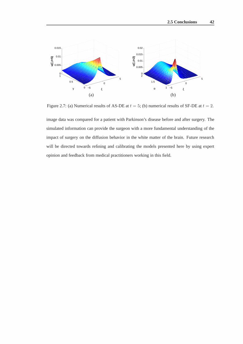
2.5 Conclusions 42
−5
0
5
0
0.5
10
0.005
0.01
0.015
ξγ
u(ξ
,t=5
)
(a)
−5
0
5
1
1.5
20
0.005
0.01
0.015
0.02
ξα
u(ξ
,t=2
)
(b)
Figure 2.7: (a) Numerical results of AS-DE att = 5; (b) numerical results of SF-DE att = 2.
image data was compared for a patient with Parkinson’s disease before and after surgery. The
simulated information can provide the surgeon with a more fundamental understanding of the
impact of surgery on the diffusion behavior in the white matter of the brain. Future research
will be directed towards refining and calibrating the modelspresented here by using expert
opinion and feedback from medical practitioners working inthis field.

CHAPTER 3
Numerical simulation of the fractional Bloch equations
3.1 Introduction
Diffusion-weighted imaging is an MR imaging modality that allows the magnitude of the local
diffusion of spins in a chosen direction to be estimated in individual scan voxels. By combining
measurements in six or more directions it is possible to construct the diffusion tensor [7], which
contains information describing the anisotropy of diffusion assuming Gaussian diffusion.
In physics and chemistry, specifically in NMR (nuclear magnetic resonance) or MRI
(magnetic resonance imaging), or ESR (electron spin resonance) the Bloch equations are
a set of macroscopic equations that are used to calculate thenuclear magnetizationM =
(Mx,My,Mz) as a function of time when relaxation timesT1 and T2 are present. Here
Mx(t),My(t) andMz(t) represent the system magnetization (x, y, and z components), T1 is
the spin-lattice relaxation time characterizing the rate at which the longitudinalMz component
of the magnetization vector recovers exponentially towards its thermodynamic equilibrium,
andT2 is the spin-spin relaxation time characterizing the signaldecay in NMR and MRI.

3.1 Introduction 44
The classical Bloch equations take the following form [83, 130]:
dMx(t)
dt= ω0My(t)−
Mx(t)
T2, (3.1)
dMy(t)
dt= −ω0Mx(t)−
My(t)
T2, (3.2)
dMz(t)
dt=
M0 −Mz(t)
T1, (3.3)
whereM0 is the equilibrium magnetization, andω0 is the resonant frequency given by the
Larmor relationshipω0 = γB0, whereB0 is the static magnetic field (z-component) andγ/2π
is the gyromagnetic ratio (42.57 MHz/Tesla for water protons).
Some fractional models have been proposed for the Bloch equation. Magin et al. [83]
considered the following time-fractional Bloch equations(TFBE):
C0 D
αt Mx(t) = ω′
0My(t)−Mx(t)
T ′2
, (3.4)
C0 D
αt My(t) = −ω′
0Mx(t)−My(t)
T ′2
, (3.5)
C0 D
αt Mz(t) =
M0 −Mz(t)
T ′1
, (3.6)
whereC0 D
αt is the Caputo time fractional derivative of orderα (0 < α ≤ 1), andω′
0 =
ω0/τα−12 , 1/T ′
1 = τα−11 /T1 and 1/T ′
2 = τα−12 /T2 each have the units of(sec)−α. The
fractional time constantsτ1 and τ2 are needed to maintain a consistent set of units for the
magnetization. They used this model to study the spin dynamics and magnetization relaxation,
in the simple case of a single spin particle at resonance in a static magnetic field.
Velasco et al. [130] investigated the following anomalous fractional Bloch equations (AFBE):
dMx(t)
dt= ω0My(t)−
D1−α0+ Mx(t)
T2, (3.7)
dMy(t)
dt= −ω0Mx(t)−
D1−α0+ My(t)
T2, (3.8)
dMz(t)
dt= D1−β
0+
M0 −Mz(t)
T1, (3.9)
whereD1−α0+ andD1−β
0+ are the time fractional Riemann-Liouville derivative with0 < α ≤ 1
and0 < β ≤ 1. They used this model to fit the derived spin-spin relaxation(T2) decay curves
to relaxation data from normal and trypsin-digested bovinenasal cartilage.

3.1 Introduction 45
Magin et al. [83] and Velasco et al. [130] have demonstrated that a fractional calculus
based diffusion model can be successfully applied to analysing diffusion images of human
brain tissues and provided new insights into further investigations of tissue structures and
the microenvironment. However, effective numerical methods and supporting error analyses
for the fractional Bloch equation (FBE) are still limited. This motivates us to derive an
analytical solution and an effective numerical method for the FBE, and to study the stability
and convergence of the proposed numerical method.
We will apply an operator splitting method, which is implemented in a similar manner to
the alternating directions method, to the TFBE system (3.4)-(3.6), in which we consider one
variable at each time step, holding the others constant. At each step of the method, this reduces
the problem to the one variable equation
C0 D
αt M(t) = −K1M(t) + f(t), (3.10)
whereK1 > 0 is constant. Similarly, using an operator splitting method, the AFBE system
(3.7)-(3.9) is equivalent to solving the one variable equation
dM(t)
dt= −K2D
1−α0+ M(t) + f(t), (3.11)
whereK2 > 0 is constant. As usual we demand that the functionf be continuous and that it
fulfils a Lipschitz condition with respect to its second argument, with Lipschitz constantL on
a suitable setG.
In this chapter, we consider the time-fractional Bloch equations (TFBE) and the anomalous
fractional Bloch equations (AFBE) with an initial condition.
The structure of the remainder of this chapter as follows. InSection3.2, some mathematical
preliminaries are introduced. In Section3.3, an approximate analytical solution for the TFBE
is derived. In Section3.4, we propose an effective predictor-corrector method (PCM)for the
TFBE. The error analysis for PCM is investigated in Section3.5. In Section3.6, we propose an
implicit numerical method (INM) for the AFBE. The stabilityand convergence of the INM are
investigated in Sections3.7 and3.8, respectively. Finally, we present some numerical results
that support our theoretical analysis.

3.2 Preliminary knowledge 46
3.2 Preliminary knowledge
In this section, we outline important definitions and lemmasused throughout the remaining
sections of this chapter.
Firstly, we present the definitions of two classical Mittag-Leffler functions. More detailed
information on the Mittag-Leffler functions may be found in [38, 63, 111].
Definition 3.1. A two-parameter function of the Mittag-Leffler type is defined by the series
expansion [37]
Eα,β(z) ≡∞∑
k=0
zk
Γ(αk + β), (α > 0, β > 0).
Whenβ = 1, we obtain the Mittag-Leffler function defined in terms of oneparameter:
Eα,1(z) =
∞∑
k=0
zk
Γ(αk + 1)≡ Eα(z).
Definition 3.2. Let A ∈ Rn×n. The matrixα−Exponential functionezA
α is defined by [16, 63]
ezAα ≡ zα−1Eα,α(z
αA) = zα−1∞∑
k=0
Ak zαk
Γ[(k + 1)α],
wherez ∈ C \ 0, α > 0.
Whenα = 1, ezA1 coincides with the matrix exponential functionezA :
ezA1 = ezA , (z ∈ C).
In addition, the functionezAα satisfies the following properties [16, 63]:
Lemma 3.1. If A,B ∈ Rn×n, 0 < α ≤ 1, and let‖A‖ = max
1≤i,j≤n|aij |, we have
1. ‖ezAα ‖ ≤ |z|α−1
∞∑k=0
‖A‖k |z|αk
Γ[(k+1)α] ;
2. ezAα ezB
α 6= ez(A+B)α , (α 6= 1);
3. Ca Dαt e
zAα = AezA
α .
Furthermore, we give the definitions of two fractional derivatives.

3.3 Analytical solution of the TFBE 47
Definition 3.3. For functionsM(t) given in the interval[a, b], the expression [78, 111]
Ca D
αt M(t) =
1Γ(m−α)
∫ ta
M (m)(η)(t−η)1+α−m dη, m− 1 < α < m,
dm
dtmM(t), α = m ∈ N,
is called a time Caputo fractional derivative of orderα (m− 1 < α ≤ m).
Definition 3.4. For functionsM(t) given in the interval[a, b], the expression [73, 111]
Dαa+M(t) =
1Γ(m−α)
∂m
∂tm
∫ ta
M(ξ)dξ(t−ξ)α+1−m , m− 1 < α < m,
dm
dtmM(t), α = m ∈ N,
is called the Riemann-Liouville derivative of orderα (m− 1 < α ≤ m).
The relationship between the Riemann-Liouville and Caputofractional derivative is given in
[111] as
Dαa+M(t) =
m−1∑
j=0
M j(a)
Γ(1 + j − α)(t− a)j−α + C
a Dαt M(t).
Lemma 3.2. [31, 135] Let M ∈ Cm[0, T ] for somem ∈ N and assume that0 < α < m.
ThenC0 Dαt M ∈ C[0, T ].
The following properties of the operatorsCa Dαt andDα
a+ are detailed in [111]:
Lemma 3.3. If α ≥ 0 andγ > −1, we have
1. Ca Dαt t
γ = Γ(γ+1)Γ(γ−α+1) (t− a)γ−α;
2. Dαa+t
γ = Γ(γ+1)Γ(γ−α+1) (t− a)γ−α.
Noting that for constantC∗, Ca D
αt C
∗ = 0 and Dαa+C
∗ = C∗(t−a)−α
Γ(1−α) .
3.3 Analytical solution of the TFBE
The time-fractional Bloch equations (TFBE) (3.4)-(3.6) can be written as
C0 D
αt M(t) = AM(t) + b(t), (3.12)

3.3 Analytical solution of the TFBE 48
which satisfies
M(0) = M0, (3.13)
whereA =
−
1T ′
2
ω′
0 0
−ω′
0 −
1T ′
2
0
0 0 −
1T ′
1
∈ R
3×3, b(t) = (0, 0, M0T ′
1)T , M(t) = (Mx(t),My(t),Mz(t))
T
andM0 = (Mx(0),My(0),Mz(0))T are vectors.
Lemma 3.4. The matrix
T(t) = etAα ,(A ∈ R
n×n)
is a fundamental solution matrix for the system
C0 D
αt M (t) = AM(t).
Theorem 3.1. The following initial-value problem
C0 D
αt M(t) = AM(t),
M(0) = M0 (M0 ∈ Rn),
whereA ∈ Rn×n, has its unique continuous global solutionM(t) in [0,∞) ⊂ R given by
M(t) =
∫ t
0e(t−ξ)Aα AM0dξ + M0.
Proof. See [16, 63].
UsingCγ [a, b] (γ ∈ R) [16, 63] to denote the Banach space
Cγ [a, b] = g(t) ∈ C(a, b] : ‖g‖Cγ = ‖(t− a)γg(t)‖C < ∞,
where‖g‖C = maxt∈[a,b]
|g(t)|. In particular,C0[a, b] represents the space of continuous functions
in [a, b], namelyC[a, b].
Then, using Lemma3.1, Lemma3.2, Lemma3.4 and Theorem3.1, we can obtain an explicit
general solution of the time-fractional Bloch equations (TFBE) (3.12)-(3.13) by Theorem3.2.

3.4 An effective predictor-corrector method (PCM) for the TFBE 49
Theorem 3.2. The following initial-value problem
C0 D
αt M(t) = AM(t) + b(t),
M(0) = M0 (M0 ∈ Rn),
where A ∈ Rn×n and b ∈ C1−α[0, T ], meaning each component ofb belongs to space
C1−α[0, T ], has its unique solution given by
M(t) =
∫ t
0e(t−ξ)Aα [b(ξ) + AM0]dξ + M0
=
∫ t
0e(t−ξ)Aα b(ξ)dξ + [AtαEα,α+1(t
αA) + I] M0.
Proof. See [16, 63].
3.4 An effective predictor-corrector method (PCM) for the TFBE
We propose an effective predictor-corrector method (PCM) for the following time-fractional
Bloch equation (TFBE) with initial condition:
C0 D
αt M(t) = −K1M(t) + f(t), (3.14)
M(0) = M#0 , (3.15)
where0 < α ≤ 1, andK1 > 0, M#0 are constants.
It is well known that the initial value problem (3.14)-(3.15) is equivalent to the Volterra integral
equation
M(t) = M#0 +
1
Γ(α)
∫ t
0(t− ξ)α−1[−K1M(ξ) + f(ξ)]dξ.
For the sake of simplicity, we assume that we are working witha uniform temporal discrete
schemetj = jτ, j = 0, 1, · · · , n, andnτ = T , whereT represents the final time.
It is known that the classical Adams-Bashforth-Moulton method for first order ordinary
differential equations is a reasonable and practically useful compromise in the sense that
its stability properties allow for a safe application to mildly stiff equations without undue

3.4 An effective predictor-corrector method (PCM) for the TFBE 50
propagation of rounding error, whereas the implementationdoes not require extremely time
consuming elements [49]. Thus, a fractional Adams-Bashforth method and a fractional Adams-
Moulton method are chosen as our predictor and corrector formulas.
The predictorMpk+1 is determined by the fractional Adams-Bashforth method [32, 31, 135]:
Mpk+1 = M#
0 +1
Γ(α)
k∑
j=0
bj,k+1[−K1Mj + f(tj)], (3.16)
where
bj,k+1 =τα
α[(k + 1− j)α − (k − j)α]. (3.17)
Remark 3.1. [32] bj,k+1 > 0 for all j andk, and
k∑
j=0
bj,k+1 =
∫ tk+1
0(tk+1 − t)α−1dt =
1
αtαk+1 ≤
1
αTα.
The fractional Adams-Moulton method determines the corrector formula [32, 31, 135]:
Mk+1 = M#0 +
1
Γ(α)(
k∑
j=0
aj,k+1[−K1Mj+f(tj)]+ak+1,k+1[−K1Mpk+1+f(tk+1)]), (3.18)
where
aj,k+1 =τα
α(α + 1)
kα+1 − (k − α)(k + 1)α, j = 0,
(k − j + 2)α+1 + (k − j)α+1 − 2(k − j + 1)α+1, 1 ≤ j ≤ k,
1, j = k + 1.
(3.19)
Remark 3.2. [32] aj,k+1 > 0 for all j andk, and
k∑
j=0
aj,k+1 =
∫ tk
0(tk − t)α−1dt =
1
αtαk ≤ 1
αTα.
This method has been used for parameter estimation of fractional dynamical models arising
from biological systems [75].
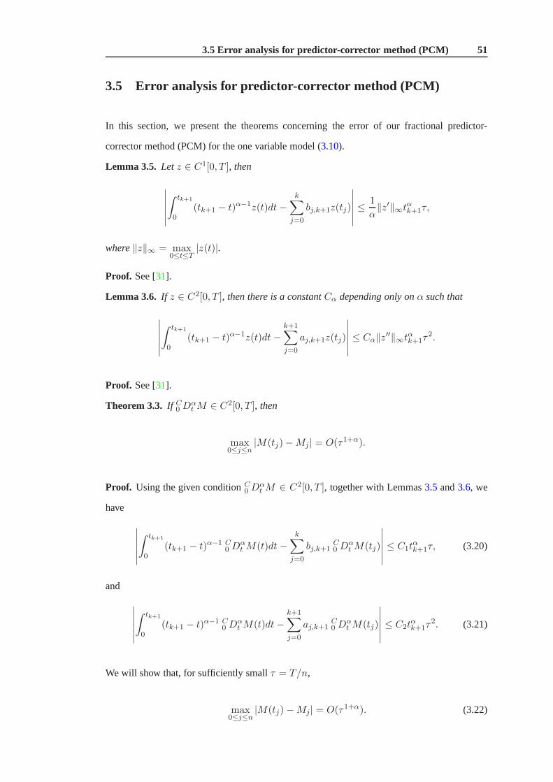
3.5 Error analysis for predictor-corrector method (PCM) 51
3.5 Error analysis for predictor-corrector method (PCM)
In this section, we present the theorems concerning the error of our fractional predictor-
corrector method (PCM) for the one variable model (3.10).
Lemma 3.5. Letz ∈ C1[0, T ], then
∣∣∣∣∣∣
∫ tk+1
0(tk+1 − t)α−1z(t)dt−
k∑
j=0
bj,k+1z(tj)
∣∣∣∣∣∣≤ 1
α‖z′‖∞tαk+1τ,
where‖z‖∞ = max0≤t≤T
|z(t)|.
Proof. See [31].
Lemma 3.6. If z ∈ C2[0, T ], then there is a constantCα depending only onα such that
∣∣∣∣∣∣
∫ tk+1
0(tk+1 − t)α−1z(t)dt−
k+1∑
j=0
aj,k+1z(tj)
∣∣∣∣∣∣≤ Cα‖z′′‖∞tαk+1τ
2.
Proof. See [31].
Theorem 3.3. If C0 D
αt M ∈ C2[0, T ], then
max0≤j≤n
|M(tj)−Mj | = O(τ1+α).
Proof. Using the given conditionC0 Dαt M ∈ C2[0, T ], together with Lemmas3.5 and3.6, we
have
∣∣∣∣∣∣
∫ tk+1
0(tk+1 − t)α−1 C
0 Dαt M(t)dt−
k∑
j=0
bj,k+1C0 D
αt M(tj)
∣∣∣∣∣∣≤ C1t
αk+1τ, (3.20)
and
∣∣∣∣∣∣
∫ tk+1
0(tk+1 − t)α−1 C
0 Dαt M(t)dt−
k+1∑
j=0
aj,k+1C0 D
αt M(tj)
∣∣∣∣∣∣≤ C2t
αk+1τ
2. (3.21)
We will show that, for sufficiently smallτ = T/n,
max0≤j≤n
|M(tj)−Mj| = O(τ1+α). (3.22)

3.5 Error analysis for predictor-corrector method (PCM) 52
The proof will be based on mathematical induction. In view ofthe given initial condition, the
induction basis(j = 0) is presupposed.
Now assume that (3.22) is true forj = 0, 1, · · · , k(k ≤ n− 1), that is
max0≤j≤k
|M(tj)−Mj| = O(τ1+α). (3.23)
We must then prove that the inequality also holds forj = k+1. To do this, we first look at the
error of the predictorMpk+1. By construction of the predictor, using (3.20), assumption (3.23),
Remark3.1, and−K1M(t) + f(t) fulfils a Lipschitz condition, we find that
|M(tk+1)−Mpk+1|
=1
Γ(α)
∣∣∣∣∣∣
∫ tk+1
0(tk+1 − t)α−1[−K1M(t) + f(t)]dt−
k∑
j=0
bj,k+1[−K1Mj + f(tj)]
∣∣∣∣∣∣
≤ 1
Γ(α)
∣∣∣∣∣∣
∫ tk+1
0(tk+1 − t)α−1 C
0 Dαt M(t)dt−
k∑
j=0
bj,k+1C0 D
αt M(tj)
∣∣∣∣∣∣
+1
Γ(α)
k∑
j=0
bj,k+1|[−K1M(tj) + f(tj)]− [−K1Mj + f(tj)]|
≤C1t
αk+1
Γ(α)τ +
1
Γ(α)
k∑
j=0
bj,k+1LCτ1+α
≤ C1Tα
Γ(α)τ +
CLTα
Γ(α+ 1)τ1+α. (3.24)
On the basis of the bound (3.24) for the predictor error, we begin the analysis of the corrector
error. We recall the relation (3.19) which we shall use, in particular, forj = k + 1 and
arguing in a similar way to the above, using (3.21), (3.24), assumption (3.23), Remark3.2, and

3.6 Implicit numerical method for the AFBE 53
−K1M(t) + f(t) fulfils a Lipschitz condition, we find that
|M(tk+1)−Mk+1|
=1
Γ(α)
∣∣∣∣∫ tk+1
0(tk+1 − t)α−1[−K1M(t) + f(t)]dt
−k∑
j=0
aj,k+1[−K1Mj + f(tj)]− ak+1,k+1[−K1Mpk+1 + f(tk+1)]
∣∣∣∣∣∣
≤ 1
Γ(α)
∣∣∣∣∣∣
∫ tk+1
0(tk+1 − t)α−1 C
0 Dαt M(t)dt−
k+1∑
j=0
aj,k+1C0 D
αt M(tj)
∣∣∣∣∣∣
+1
Γ(α)
k∑
j=0
aj,k+1|[−K1M(tj) + f(tj)]− [−K1Mj + f(tj)]|
+1
Γ(α)ak+1,k+1|[−K1M(tk+1) + f(tk+1)]− [−K1M
pk+1 + f(tk+1)]|
≤C2t
αk+1
Γ(α)τ2 +
CL
Γ(α)τ1+α
k∑
j=0
aj,k+1 + ak+1,k+1L
Γ(α)
(C1T
α
Γ(α)τ +
CLTα
Γ(α+ 1)τ1+α
)
≤(C2T
α
Γ(α)+
CLTα
Γ(α+ 1)+
C1LTα
Γ(α)Γ(α + 2)+
CL2Tα
Γ(α+ 1)Γ(α + 2)τα)τ1+α
≤ C0τ1+α.
Thus, we now see that the induction step is completed and the result is true for allj.
3.6 Implicit numerical method for the AFBE
In this section, we propose an implicit numerical method (INM) for the following anomalous
fractional Bloch equations (AFBE) with initial condition:
dM(t)
dt= −K2D
1−α0+ M(t) + f(t), 0 ≤ t ≤ T, (3.25)
M(0) = M∗0 , (3.26)
whereK2 > 0 andM∗0 are constants, andD1−α
0+ (0 < α ≤ 1) is the time fractional Riemann-
Liouville derivative and can be written as [111]
D1−α0+ M(t) =
∂
∂tIα0 M(t),

3.6 Implicit numerical method for the AFBE 54
whereIα0 M(t) = 1Γ(α)
∫ t0
M(η)dη(t−η)1−α is the Riemann-Liouville fractional integral of orderα > 0.
Let t = tk = kτ(k = 0, 1, · · · , n), whereτ = T/n is the time step size.
We introduce the following numerical approximation
Iα0 M(tk) =1
Γ(α)
∫ tk
0
M(η)
(tk − η)1−αdη
=1
Γ(α)
k−1∑
j=0
∫ tj+1
tj
M(η)
(tk − η)1−αdη
=1
Γ(α)
k−1∑
j=0
∫ tj+1
tj
M(tj+1) +M ′(ηj)(η − tj+1)
(tk − η)1−αdη
=τα
Γ(α+ 1)
k−1∑
j=0
bjM(tk−j) + Ckατ1+α max0≤t≤T
|M ′(t)|,
wheretj < ηj < tj+1, andbj = (j + 1)α − jα, j = 0, 1, · · · , n− 1.
Thus, we have
Lemma 3.7. If M(t) ∈ C1[0, T ], then
Iα0 M(tk) =τα
Γ(α+ 1)
k−1∑
j=0
bjM(tk−j) +Rαk ,
where|Rαk | ≤ Ctαk τ .
Lemma 3.8. The coefficientsbj satisfy:
1. bj > 0 for j = 0, 1, 2, · · · ;
2. 1 = b0 > b1 > · · · > bn, bn → 0 asn → ∞;
3. There exists a positive constantC > 0, such thatτ ≤ Cbjτα, j = 1, 2, · · · ;
4.k∑
j=0bjτ
α = (k + 1)ατα ≤ Tα.
Proof. See [157].
Using Lemmas3.7and3.8, we have the following Lemma.
Lemma 3.9. If M(t) ∈ C2[0, T ], then
Iα0 M(tk+1)−Iα0 M(tk) =τα
Γ(α+ 1)
bkM(t1) +
k−1∑
j=0
bk−j−1[M(tj+2)−M(tj+1)]
+Rk,α,

3.7 Stability of the implicit numerical method for the AFBE 55
where|Rk,α| ≤ Cbkτ1+α.
Proof. See [77].
Integrating both sides of Eq.(3.25) from tk to tk+1, we have
M(tk+1)−M(tk) = −K2[Iα0 M(tk+1)− Iα0 M(tk)] +
∫ tk+1
tk
f(t)dt.
Thus, using Lemma3.9we have
M(tk+1) = M(tk)− r
bkM(t1)−
k−1∑
j=0
bk−j−1[M(tj+2)−M(tj+1)]
+τ
2[f(tk+1) + f(tk)] +Rk+1,
or, rearranging, we obtain
M(tk+1) = M(tk)− rM(tk+1)− rk−1∑
j=0
(bj+1 − bj)M(tk−j) +τ
2[f(tk+1) + f(tk)]
+Rk+1, (3.27)
for k = 0, 1, 2, · · · , n− 1, wherer = K2τα
Γ(α+1) , and
|Rk+1| ≤ Cbkτ1+α. (3.28)
Thus, we have derived the following implicit numerical method (INM) for the initial value
problem of the anomalous fractional Bloch equations (AFBE):
Mk+1 = Mk − rMk+1 − r
k−1∑
j=0
(bj+1 − bj)Mk−j +
τ
2[f(tk+1) + f(tk)], (3.29)
k = 0, 1, 2, · · · , n− 1.
3.7 Stability of the implicit numerical method for the AFBE
In this section, we discuss the stability of the implicit numerical method for the AFBE.
Theorem 3.4. The implicit numerical method defined by Eq.(3.29) is unconditionally stable.

3.7 Stability of the implicit numerical method for the AFBE 56
Proof. We suppose thatMk(k = 0, 1, 2, · · · , n) is the approximate solution of Eq.(3.29). The
rounding errorεk = Mk −Mk satisfies
εk+1 = εk − rεk+1 − r
k−1∑
j=0
(bj+1 − bj)εk−j . (3.30)
Multiplying Eq. (3.30) by εk+1 we obtain
(εk+1)2 = εk+1εk − r(εk+1)2 − r
k−1∑
j=0
(bj+1 − bj)εk−jεk+1.
Using the inequality±εk−jεk+1 ≤ 12
[(εk−j)2 + (εk+1)2
], we have
(εk+1)2 ≤ 1
2
[(εk+1)2 + (εk)2
]− r(εk+1)2 +
r
2
k−1∑
j=0
(bj − bj+1)[(εk−j)2 + (εk+1)2
].
Using Lemma3.8and notingb0 = 1, we have
k−1∑
j=0
(bj − bj+1) = 1− bk,
and
(εk+1)2 ≤ 1
2
[(εk+1)2 + (εk)2
]− r
2(1 + bk)(ε
k+1)2 +r
2
k−1∑
j=0
(bj − bj+1)(εk−j)2
≤ 1
2
[(εk+1)2 + (εk)2
]− r
2(εk+1)2 +
r
2
k−1∑
j=0
(bj − bj+1)(εk−j)2.
Therefore, we obtain
(εk+1)2 + rk∑
j=0
bj(εk+1−j)2 ≤ (εk)2 + r
k−1∑
j=0
bj(εk−j)2.
Let
(εk)2E = (εk)2 + rk−1∑
j=0
bj(εk−j)2,

3.8 Convergence of the implicit numerical method for the AFBE 57
we obtain the result
(εk+1)2 ≤ (εk+1)2E ≤ (εk)2E ≤ · · · ≤ (ε1)2E ≤ (ε0)2E = (ε0)2.
Hence, the proof of Theorem3.4 is completed.
3.8 Convergence of the implicit numerical method for the AFBE
Let M(tk)(k = 0, 1, 2, · · · , n) be the exact solution of the anomalous fractional Bloch
equations (AFBE) (3.25)-(3.26) at mesh pointtk. Define ηk = M(tk) − Mk(k =
0, 1, 2, · · · , n).
We will prove the following theorem of convergence.
Theorem 3.5. The implicit numerical method defined by Eq.(3.25) is convergent, and there
exists a positive constantC∗ > 0, such that
|ηk+1| ≤ C∗τ, k = 0, 1, 2, · · · , n − 1,
whereτ is the time step.
Proof. From Eq. (3.27) and Eq. (3.29), we have
ηk+1 = ηk − rηk+1 − r
k−1∑
j=0
(bj+1 − bj)ηk−j +Rk+1, (3.31)
k = 0, 1, 2, · · · , n − 1.
Multiplying Eq. (3.31) by ηk+1 and using the Cauchy-Schwartz inequality we obtain
(ηk+1)2 = ηk+1ηk − r(ηk+1)2 − r
k−1∑
j=0
(bj+1 − bj)ηk−jηk+1 +Rk+1η
k+1
≤ 1
2
[(ηk+1)2 + (ηk)2
]− r
2(1 + bk)(η
k+1)2 +r
2
k−1∑
j=0
(bj − bj+1)(ηk−j)2
+Rk+1ηk+1.

3.9 Numerical results 58
Let
(ηk)2E = (ηk)2 + r
k−1∑
j=0
bj(ηk−j)2,
Using the resultuv ≤ σu2 + 14σv
2, σ > 0, we have
Rk+1ηk+1 ≤ rbk
2(ηk+1)2 +
1
2rbk(Rk+1)
2.
Therefore, using Lemma3.8, we obtain
(ηk+1)2E = (ηk+1)2 + r
k∑
j=0
bj(ηk+1−j)2
≤ (ηk)2 + r
k−1∑
j=0
bj(ηk−j)2 − r
2bk(η
k+1)2 +Rk+1ηk+1
= (ηk)2E − r
2bk(η
k+1)2 +Rk+1ηk+1
≤ (ηk)2E − r
2bk(η
k+1)2 +rbk2
(ηk+1)2 +1
2rbk(Rk+1)
2
≤ (ηk)2E + Cbkτ2+α
≤ (η0)2E + Ck∑
j=0
bkτατ2
≤ (C∗τ)2,
i.e. |ηk+1| ≤ |ηk+1|E ≤ C∗τ . Hence, the proof of Theorem3.5is completed.
3.9 Numerical results
In this section, we present some numerical examples that support our theoretical analysis.
Example 3.1. In order to show the efficiency of the predictor-corrector method (PCM), we
consider the following time-fractional Bloch equation (TFBE) with initial condition:
C0 D
αt M(t) = −K1M(t) + f(t), 0 ≤ t ≤ T,
M(0) = 0,
where0 < α ≤ 1,K1 > 0, andf(t) = K1tα + Γ(1 + α).

3.9 Numerical results 59
0 1 2 3 4 50
0.5
1
1.5
2
2.5
3
3.5
time t
M(t
)
exact solutionnumerical solution using PCM
Figure 3.1: Comparison of the exact solution of TFBE and the numerical solution using PCMfor α = 0.7,K1 = 1.
The exact solution of this problem isM(t) = tα, which can be verified by direct fractional
differentiation of the given solution using Lemma3.3, and substituting in the fractional
differential equation. The initial condition is clearly satisfied.
Whenα = 0.7,K1 = 1, Figure3.1 shows the numerical solution obtained by applying the
predictor-corrector method (PCM) (3.16)-(3.19) and the exact solution of TFBE. It can be seen
that the numerical solution is in excellent agreement with the exact solution.
Example 3.2. Consider the following time-fractional Bloch equations (TFBE) [83] :
C0 D
αt Mx(t) = ω′
0My(t)−Mx(t)
T ′2
,
C0 D
αt My(t) = −ω′
0Mx(t)−My(t)
T ′2
,
C0 D
αt Mz(t) =
M0 −Mz(t)
T ′1
,
with initial condition
Mx(0) = 0,
My(0) = 100,
Mz(0) = 0,
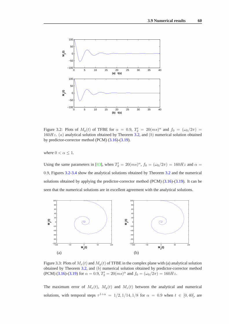
3.9 Numerical results 60
0 5 10 15 20 25 30 35 40−100
−50
0
50
100
(a) t(s)
My(t
)
0 5 10 15 20 25 30 35 40−100
−50
0
50
100
(b) t(s)
My(t
)
Figure 3.2: Plots ofMy(t) of TFBE for α = 0.9, T ′2 = 20(ms)α and f0 = (ω0/2π) =
160Hz. (a) analytical solution obtained by Theorem3.2, and(b) numerical solution obtainedby predictor-corrector method (PCM) (3.16)-(3.19).
where0 < α ≤ 1.
Using the same parameters in [83], whenT ′2 = 20(ms)α, f0 = (ω0/2π) = 160Hz andα =
0.9, Figures3.2-3.4 show the analytical solutions obtained by Theorem3.2 and the numerical
solutions obtained by applying the predictor-corrector method (PCM) (3.16)-(3.19). It can be
seen that the numerical solutions are in excellent agreement with the analytical solutions.
−100 −50 0 50 100−100
−80
−60
−40
−20
0
20
40
60
80
100
Mx(t)
My(t
)
(a)
−100 −50 0 50 100−100
−80
−60
−40
−20
0
20
40
60
80
100
Mx(t)
My(t
)
(b)
Figure 3.3: Plots ofMx(t) andMy(t) of TFBE in the complex plane with (a) analytical solutionobtained by Theorem3.2, and(b) numerical solution obtained by predictor-corrector method(PCM) (3.16)-(3.19) for α = 0.9, T ′
2 = 20(ms)α andf0 = (ω0/2π) = 160Hz.
The maximum error ofMx(t), My(t) and Mz(t) between the analytical and numerical
solutions, with temporal stepsτ1+α = 1/2, 1/14, 1/8 for α = 0.9 when t ∈ [0, 40], are

3.9 Numerical results 61
−100−50
050
100
−100
−50
0
50
1000
20
40
60
80
100
Mx(t)M
y(t)
Mz(t
)
(a)
−100−50
050
100
−100
−50
0
50
1000
20
40
60
80
100
Mx(t)M
y(t)
Mz(t
)
(b)
Figure 3.4: A Plot of numerical solutions of TFBE with (a) analytical solution obtained byTheorem3.2, and(b) numerical solution obtained by predictor-corrector method (PCM) (3.16)-(3.19) for α = 0.9, T ′
2 = 20(ms)α andf0 = (ω0/2π) = 160Hz.
Table 3.1: Comparison of maximum error ofMx(t) between the analytical and numericalsolutions forα = 0.9 whent ∈ [0, 40]
τ1+α Maximum error ofMx(t) Error rate12 8.275410 -14 3.977148 2.08≈ 218 1.901265 2.09≈ 2
listed in Tables3.1-3.3.
From Tables3.1-3.3, it can be seen that
Error rate =error1error2
≈ τ1τ2
= 2.
Thus, we obtain that the order of convergence of the numerical method PCM is(log22 = 1)
first order, that is, the convergence order of the numerical method PCM for this problem is
O(τ1+α). This is in good agreement with our theoretical analysis.
Figure 3.5(a)-(c) show plots ofMy(t) obtained by applying the predictor-corrector method
(PCM) (3.16)-(3.19) for the values of(a) α = 1.0, (b) α = 0.9 and(c) α = 0.8 for a spin
Table 3.2: Comparison of maximum error ofMy(t) between the analytical and numericalsolutions forα = 0.9 whent ∈ [0, 40]
τ1+α Maximum error ofMy(t) Error rate12 6.281390 -14 3.154087 1.99≈ 218 1.563063 2.02≈ 2

3.9 Numerical results 62
Table 3.3: Comparison of maximum error ofMz(t) between the analytical and numericalsolutions forα = 0.9 whent ∈ [0, 40]
τ1+α Maximum error ofMz(t) Error rate12 0.000126 -14 0.000032 1.88≈ 218 0.000014 2.09≈ 2
0 5 10 15 20 25 30 35 40−100
0
100
My(t
)
(a) t(s)
0 5 10 15 20 25 30 35 40−100
0
100
My(t
)
(b) t(s)
0 5 10 15 20 25 30 35 40−50
0
50
100
My(t
)
(c) t(s)
Figure 3.5: Plots ofMy(t) of TFBE for T ′2 = 20(ms)α andf0 = (ω0/2π) = 160Hz and
(a) α = 1.0, (b) α = 0.9 and(c) α = 0.8 top to bottom, respectively.
system.
To illustrate the dynamic relationship between theMx(t) andMy(t) for fractional and the
integer order relaxation, these two components of magnetization obtained by applying the
predictor-corrector method (PCM) (3.16)-(3.19) are plotted in the complex plane, as shown
in Figure3.6. Figure3.6(a) the classical case ofα = 1 shows a regular spiral from the initial
valuesMx(0) = 0 andMy(0) = 100 into the origin (center of the plot) [83]. Figure3.6(b) and
Figure3.6(c) show a much faster decay for the chosen values ofT ′2 for α = 0.9 andα = 0.8,
respectively. Figures3.7 and3.8 show the entire trajectory of magnetization for both cases
in three dimensions with the magnetization starting atMx(0) = 0 andMy(0) = 100 and
returning to its equilibrium value ofM0.
Example 3.3. Consider the following anomalous fractional Bloch equations (AFBE) with

3.9 Numerical results 63
−100 −50 0 50 100−100
−80
−60
−40
−20
0
20
40
60
80
100
Mx(t)
My(t
)
(a)
−100 −50 0 50 100−100
−80
−60
−40
−20
0
20
40
60
80
100
Mx(t)
My(t
)
(b)
−100 −50 0 50 100−100
−80
−60
−40
−20
0
20
40
60
80
100
Mx(t)
My(t
)
(c)
Figure 3.6: Plots ofMx(t) andMy(t) of TFBE in the complex plane withα = 1 (a, classicalmodel),α = 0.9 (b) andα = 0.8 (c) for T ′
2 = 20(ms)α andf0 = (ω0/2π) = 160Hz.
initial condition:
dM(t)
dt= −K2D
1−α0+ M(t) + f(t), 0 ≤ t ≤ T,
M(0) = 0,
where0 < α ≤ 1,K2 > 0, andf(t) = (1 + α)tα + K2Γ(2+α)Γ(1+2α) t2α.
The exact solution of this problem isM(t) = t1+α , which can be verified by direct fractional
differentiation of the given solution using Lemma3.3, and substituting in the fractional
differential equation. The initial condition is clearly satisfied.
Whenα = 0.7,K2 = 1, Figure3.9 shows the numerical solution obtained by applying the
implicit numerical method (INM) (3.29) and the exact solution of AFBE. It can be seen that
the numerical solution is in excellent agreement with the exact solution.
Example 3.4. Consider the following anomalous fractional Bloch equations (AFBE) with

3.9 Numerical results 64
−100−50
050
100
−100
−50
0
50
1000
20
40
60
80
100
Mx(t)M
y(t)
Mz(t
)
Figure 3.7: A Plot of numerical solutions of TFBE using the predictor-corrector method (PCM)with α = 1 (classical model) forT ′
1 = 100(ms)α, T ′2 = 20(ms)α andf0 = (ω0/2π) =
160Hz.
−100−50
050
100
−100
−50
0
50
1000
20
40
60
80
100
Mx(t)M
y(t)
Mz(t
)
Figure 3.8: Plots of numerical solutions of TFBE using the predictor-corrector method (PCM)with α = 0.9 (fractional model) forT ′
1 = 100(ms)α, T ′2 = 20(ms)α andf0 = (ω0/2π) =
160Hz.

3.9 Numerical results 65
0 1 2 3 4 50
2
4
6
8
10
12
14
16
time t
M(t
)
exact solutionimplicit numerical solution
Figure 3.9: Comparison of the exact solution of AFBE and the numerical solution using INMfor α = 0.7,K2 = 1.
initial condition:
dMx(t)
dt= ω0My(t)−
D1−α0+ Mx(t)
T2,
dMy(t)
dt= −ω0Mx(t)−
D1−α0+ My(t)
T2,
dMz(t)
dt= D1−β
0+
M0
T1−D1−β
0+
Mz(t)
T1,
with initial condition
Mx(0) = 0,
My(0) = 100,
Mz(0) = 0,
where0 < α ≤ 1.
WhenT2 = 20(ms) andf0 = (ω0/2π) = 160Hz, Figure3.10(a)-(c) show plots ofMy(t)
obtained by applying the implicit numerical method (INM) (3.29) for the values of(a) α = 1.0,
(b) α = 0.9 and(c) α = 0.8 for a spin system.
Figure3.11 shows the dynamic relationship between theMx(t) andMy(t) with the chosen

3.10 Conclusions 66
0 50 100 150 200−200
0
200
(a) t(s)M
y(t)
0 50 100 150 200−200
0
200
(b) t(s)
My(t
)
0 50 100 150 200−200
0
200
(c) t(s)
My(t
)
Figure 3.10: Plots ofMy(t) of AFBE for T2 = 20(ms) andf0 = (ω0/2π) = 160Hz and(a) α = 1.0, (b) α = 0.9 and(c) α = 0.8 top to bottom, respectively.
values ofT2 for α = β = 1.0, 0.9 and0.8, respectively. Figures3.12-3.14exhibit the entire
trajectory of magnetization in three dimensions with the magnetization starting atMx(0) = 0
andMy(0) = 100 and returning to its equilibrium value ofM0 for α = β = 1.0, 0.9 and0.8,
respectively.
3.10 Conclusions
In this chapter, an analytical solution and an effective predictor-corrector method (PCM) for
solving the time-fractional Bloch equations (TFBE) have been derived. The error analysis
for PCM is discussed. In addition, an effective implicit numerical method (INM) for solving
the anomalous fractional Bloch equations (AFBE) has been proposed. The stability and
convergence of the INM are analysed systematically. We alsopresented some numerical
examples to demonstrate the effectiveness of PCM and INM. The results show that the spin
dynamics are generally fractional order, although become the classical case when the order
of differentiation is one, and suggest that the fractional models can effectively simulate the
spin dynamics in a static magnetic field, and can play an important role for us understanding
NMR for complex systems. These numerical techniques can also be applied to simulate
other fractional order differential system, and thereforewe feel our methods have broader
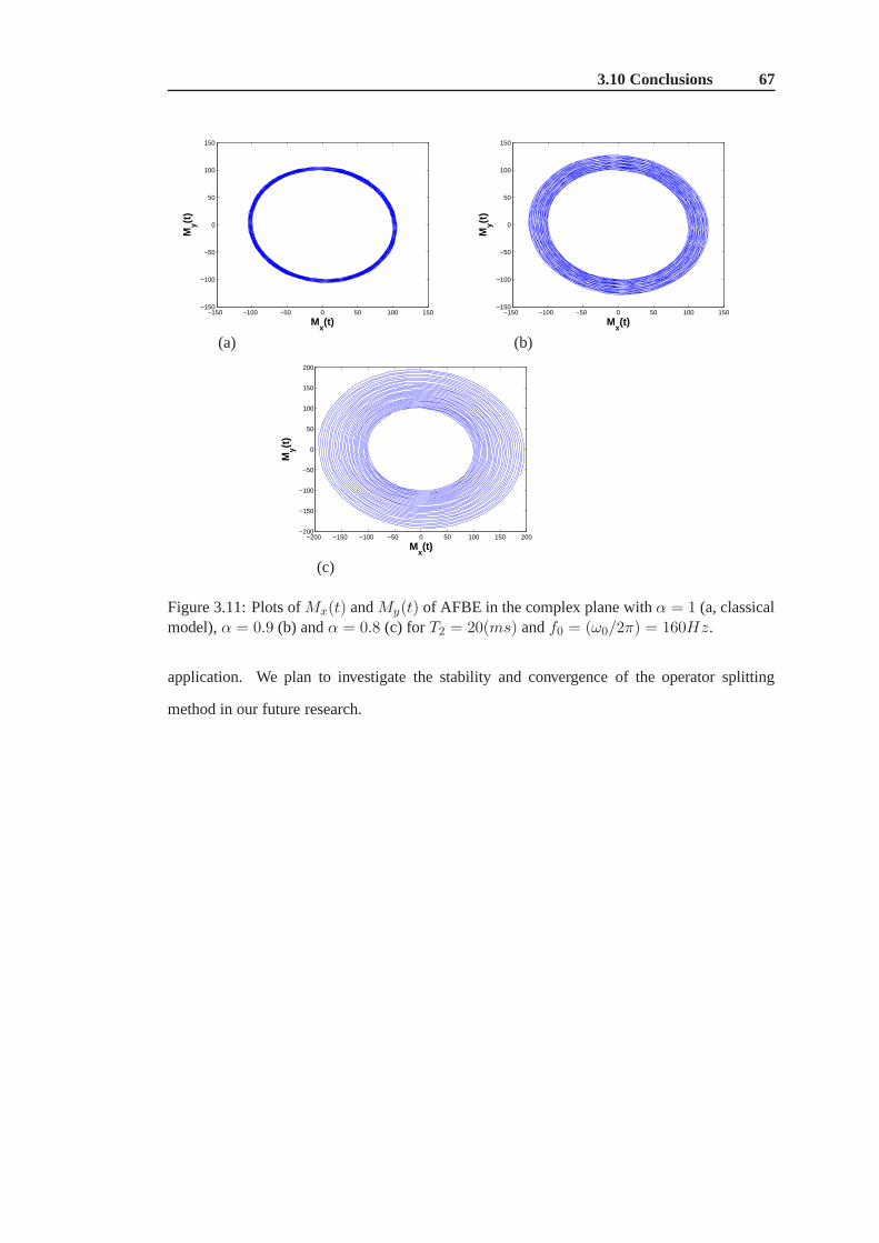
3.10 Conclusions 67
−150 −100 −50 0 50 100 150−150
−100
−50
0
50
100
150
Mx(t)
My(t
)
(a)
−150 −100 −50 0 50 100 150−150
−100
−50
0
50
100
150
Mx(t)
My(t
)
(b)
−200 −150 −100 −50 0 50 100 150 200−200
−150
−100
−50
0
50
100
150
200
Mx(t)
My(t
)
(c)
Figure 3.11: Plots ofMx(t) andMy(t) of AFBE in the complex plane withα = 1 (a, classicalmodel),α = 0.9 (b) andα = 0.8 (c) for T2 = 20(ms) andf0 = (ω0/2π) = 160Hz.
application. We plan to investigate the stability and convergence of the operator splitting
method in our future research.

3.10 Conclusions 68
−200−100
0100
200
−200
−100
0
100
2000
20
40
60
80
100
Mx(t)M
y(t)
Mz(t
)
Figure 3.12: A Plot of numerical solutions of AFBE using the implicit numerical method (INM)with α = β = 1 (classical model) forT1 = 100(ms), T2 = 20(ms) andf0 = (ω0/2π) =160Hz.
−200−100
0100
200
−200
−100
0
100
2000
20
40
60
80
100
Mx(t)M
y(t)
Mz(t
)
Figure 3.13: A Plot of numerical solutions of AFBE using the implicit numerical method (INM)with α = β = 0.9 (fractional model) forT1 = 100(ms), T2 = 20(ms) andf0 = (ω0/2π) =160Hz.

3.10 Conclusions 69
−200−100
0100
200
−200
−100
0
100
2000
20
40
60
80
100
Mx(t)M
y(t)
Mz(t
)
Figure 3.14: A Plot of numerical solutions of TFBE using the implicit numerical method (INM)with α = β = 0.8 (fractional model) forT1 = 100(ms), T2 = 20(ms) andf0 = (ω0/2π) =160Hz.

CHAPTER 4
Stability and convergence of an implicit numerical
method for the space and time fractional Bloch-Torrey
equation
4.1 Introduction
Fractional calculus has been widely used in recent years in various applications in science and
engineering. Fractional order dynamics in physics, particularly when applied to diffusion, leads
to an extension of the concept of Brownian motion through a generalization of the Gaussian
probability function to what is termed anomalous diffusion[14, 82, 83, 130]. A particular and
very interesting class of complex phenomena arises in nuclear magnetic resonance (NMR) and
magnetic resonance imaging (MRI). Here fractional calculus may help to express a physical
meaning through the fractional order of the derivative operator.
As MRI is applied with increasing temporal and spatial resolution, the spin dynamics
are being examined more closely; such examinations extend our knowledge of biological
materials through a detailed analysis of the relaxation time distribution and water diffusion

4.1 Introduction 71
heterogeneity [82]. In many biological tissues, the diffusion-induced MR signal loss deviates
from monoexponential decay,exp(−bD) (whereD is the diffusion coefficient andb is the
b-factor), particularly at highb values (for example,> 1500s/mm2 for human brain tissues)
[66]. This phenomenon is sometimes referred to as anomalous diffusion, and several analytical
models of non-monoexponential decay have been suggested [62, 102]. A common assumption
is that diffusion in two or more compartments is being observed with the compartments
representingfast (extracellular) andslow (intracellular) components to the signal. Thefast
component dominates at lowb values, and theslow at higherb values [29], leading to a
biexponential form for the signal decayS(b), with a different value for the diffusion constant
in each compartment
S(b) = S(0)(fe−bDfast + (1− f)e−bDslow), (4.1)
whereDfast > Dslow are the diffusion constants in each compartment andf the volume
fraction for the fast compartment.
Although intuitively appealing, there are several difficulties associated with the biexponential
model. First, fitting the biexponential curve is nontrivial. It is a nonlinear fitting problem where
different parameter combinations can lead to similar fits. Additionally, observed compartment
sizes do not correspond to known volume fractions of intra toextracellular space in analysed
brain tissue microstructure [29, 100]. Furthermore, in vitro experiments involving images of
single oocytes also reveal non-monoexponential behavior from the intracellular contribution
alone [121], suggesting fractions obtained from biexponential fitting do not correspond to intra
and extracellular volume fractions.
Pfeuffer et al. [110] generalized the biexponential decay to a multicompartmental model:
S(b) = S(0)
n∑
i=1
fie−bDi , (4.2)
wherefi is the volume fraction of theith compartment and the sum offi satisfiesn∑
i=1
fi = 1.
The increased number of compartments provides additional degrees of freedom to fit the
experimental data. However, the quality of the fit is not necessarily improved partly due to
the increased complexity in nonlinear fitting. Yablonskiy et al. [134] further generalized this

4.1 Introduction 72
model by replacing the discrete diffusion coefficients witha continuous distribution described
by a probability functionp(D). Using this model, the average cell size has been quantitatively
related to measurable diffusion parameters. The exact expression ofp(D), however, is
unknown. The assumption of a Gaussian distribution cannot be generalized to all tissue types,
considering the heterogeneous nature of tissue complexity. Instead of explicitly deriving an
expression forp(D), Bennett et al. [12] used a stretched exponential model (Eq. (4.3)) to
describe the diffusion-induced signal loss:
S(b) = S(0)e−(b×DDC)α , (4.3)
where DDC, coined as the distributed diffusion coefficient,is a single number representation of
the diffusion coefficient distribution functionp(D), andα is an empirical constant(0 < α ≤
1). It has been demonstrated that the stretched exponential function not only fits the diffusion
data from human brain tissues more precisely but also can be used to infer microscopic
tissue structures throughα, the so-called heterogeneity index [12]. The empirical stretched
exponential function was recently derived independently by Ozarslan et al. [105] and Hall and
Barrick [50], using concepts established for anomalous diffusion and fractal models.
Anomalous diffusion refers to models of diffusion in which the environment is not locally
homogeneous, involving disorder that is not well-approximated by assuming a uniform change
in diffusion constant. Such systems include diffusion in complicated structures such as porous
or fractal media. In the study performed by Hall and Barrick [50], the stretched exponential
formalism was derived by recognizing that (a) the mean squared displacement⟨r2(t)
⟩of
diffusing molecules is related to diffusion timet by Eq. (4.4); and (b) the dependence of
apparent diffusion coefficient onb can be expressed analogously to the dependence of diffusion
coefficient ont (Eq. (4.5)),
⟨r2(t)
⟩∝ tα, (4.4)
ADC(b) ∝⟨R2(b)
⟩
b, (4.5)
where⟨R2(b)
⟩is the apparent mean-squared displacement, analogous to
⟨r2(t)
⟩. Equations (4.4)
and (4.5) directly lead to the stretched exponential expression described by Eq. (4.3).

4.1 Introduction 73
At present, a growing number of works in science and engineering deal with dynamical systems
described by fractional-order equations that involve derivatives and integrals of non-integer
order [5, 30, 47, 90, 147]. These new models are more adequate than the previously used
integer-order models, because fractional order derivatives and integrals enable the description
of the memory and hereditary properties of different substances [111]. This is the most
significant advantage of the fractional order models in comparison with integer order models,
in which such effects are neglected. If the complex heterogeneity structure, such as the spatial
connectivity, can facilitate movement of particles withina certain scale, fast motions may no
longer obey the classical Ficks law and may indeed have a probability density function that
follows a power-law. Densities ofβ-stable type have been used to describe the probability
distribution of these motions. The resulting governing equation of these motions is similar to
the traditional diffusion equation except that the orderβ of the highest derivative is fractional.
For a large number of independent solute particles the probability propagator is replaced by
the expected concentration [73]. For example, ifC(x, t) represents the concentration of the
diffusing species in one dimension, then a space and time fractional diffusion equation of the
form:
C0 D
αt C(x, t) = Kx
∂βC(x, t)
∂|x|β , (4.6)
whereKx is the generalized diffusion coefficint,C0 Dαt is the Caputo time fractional derivative
of orderα (0 < α < 1) with respect tot and with the starting point att = 0 is defined as [111]:
C0 D
αt C(x, t) =
1
Γ(1− α)
∫ t
0
C ′(x, τ)
(t− τ)αdτ, (4.7)
andRβx = ∂βC(x,t)
∂|x|βis the Riesz fractional derivative of orderβ (1 < β ≤ 2) with respect tox,
which is defined by Eq. (4.9).
Although the success of using these fractional models to describe complex diffusion in biologic
tissues remains to be seen, they suggest a possible fractional order dynamics in the observed
diffusion-induced magnetization changes, as dictated by the Bloch-Torrey equation. Inspired
by this possibility, some authors recently examined the connection between fractional order
dynamics and diffusion by solving the Bloch-Torrey equation using fractional order calculus
[14, 82, 83, 130]. They have demonstrated that a fractional calculus based diffusion model
can be successfully applied to analysing diffusion images of human brain tissues and provide

4.1 Introduction 74
new insights into further investigations of tissue structures and the microenvironment. The
following new diffusion model was proposed for solving the Bloch-Torrey equation using
fractional order calculus with respect to time and space using the Riesz formulation [82]:
τα−1 C0 D
αt Mxy(r, t) = λMxy(r, t) +Dµ2(β−1)RβMxy(r, t), (4.8)
whereλ = −iγ(r ·G(t)), G(t) is the magnetic field gradient,γ andD are the gyromagnetic
ratio and the diffusion coefficient, respectively,r = (x, y, z). Magin et al. [82] considered
Rβ = (Rβx + Rβ
y + Rβz ) as a sequential Riesz fractional order operator in space [63].
Mxy(r, t) = Mx(r, t) + iMy(r, t), wherei =√−1, comprises the transverse components of
the magnetization;τα−1 andµ2(β−1) are the fractional order time and space constants needed
to preserve units,(0 < α ≤ 1, and1 < β ≤ 2). Magin et al. [82] have derived the analytical
solutions with fractional order dynamics in space (i.e.,α = 1, β an arbitrary real number,
1 < β ≤ 2) and time (i.e.,0 < α < 1, andβ = 2), respectively. However, effective numerical
methods and supporting error analyses for the space and timefractional Bloch-Torrey equation
(ST-FBTE) are still limited. This motivates us to derive an analytical solution of the fractional
Laplacian formulation and an effective implicit numericalmethod for the ST-FBTE in Riesz
form, and to study the stability and convergence of the proposed numerical method. We note
in passing that the Riesz and fractional Laplacian formulations are not equivalent, except for
certain special cases. For example, in one dimension with zero Dirichlet boundary conditions
and homogeneous Neumann boundary conditions, these two formulations are the same [158].
In this chapter, we consider the space and time fractional Bloch-Torrey equation with initial
and boundary conditions on a finite domain.
The structure of the remainder of this chapter as follows. InSection4.2, some mathematical
preliminaries are introduced. In Section4.3, an approximate analytical solution for the ST-
FBTE in fractional Laplacian form is derived. In Section4.4, we propose an implicit numerical
method (INM) for ST-FBTE in Riesz form. The stability and convergence of the INM are
investigated in Sections4.5 and4.6, respectively. In Section4.7, we exhibit the convergence
rate for NME for a preliminary study based on a two-dimensional example to confirm the
theoretical results reported in Section4.6.

4.2 Preliminary knowledge 75
4.2 Preliminary knowledge
In this section, we outline important definitions and lemmasused throughout the remaining
sections of this chapter. It is assumed throughout this section thatM(x, y, z, t) ∈ C3,3,3,2x,y,z,t (Ω)
for 0 < α ≤ 1 and1 < β ≤ 2, wheret ∈ [0, T ] andΩ : −∞ ≤ x, y, z ≤ +∞.
Definition 4.1. The Riesz fractional operatorRβ for n − 1 < β ≤ n on a infinite interval
−∞ ≤ x, y, z ≤ +∞ is defined as [46]
RβxM(x, y, z, t) =
∂βM(x, y, z, t)
∂|x|β = −cβ(−∞Dβx +x D
β+∞)M(x, y, z, t), (4.9)
wherecβ = 1
2 cos(πβ2), β 6= 1,
−∞DβxM(x, y, z, t) =
1
Γ(n− β)
∂n
∂xn
∫ x
−∞
M(ξ, y, z, t)dξ
(x− ξ)β+1−n, (4.10)
xDβ+∞M(x, y, z, t) =
(−1)n
Γ(n− β)
∂n
∂xn
∫ +∞
x
M(ξ, y, z, t)dξ
(ξ − x)β+1−n. (4.11)
Similarly, we can define the Riesz fractional derivativesRβyM(x, y, z, t) = ∂βM(x,y,z,t)
∂|y|βand
RβzM(x, y, z, t) = ∂βM(x,y,z,t)
∂|z|βof orderβ (1 < β ≤ 2) with respect toy andz.
Lemma 4.1. Suppose thatM(x) ∈ C3(−∞,∞), the following equality holds
∂β
∂|x|βM(x) = − 1
2 cos πβ2
[−∞Dβx + xD
β+∞]M(x), (4.12)
where1 < β ≤ 2.
Proof. See [137, 158].
Lemma 4.2. Suppose thatM(x) ∈ C3[0, L], the following equality
∂β
∂|x|βM(x) = − 1
2 cos πβ2
[0Dβx + xD
βL]M
∗(x), (4.13)
also holds when setting
M∗(x) =
M(x), x ∈ (0, L),
0, x /∈ (0, L),

4.2 Preliminary knowledge 76
i.e.,M∗(x) = 0 on the boundary points and beyond the boundary points.
Proof. See [137, 158].
Definition 4.2. [81] A real or complex-valued functionf(x), x > 0, is said to be in the space
Cα, α ∈ R, if there exists a real numberp > α such that
f(x) = xpf1(x) (4.14)
for a functionf1(x) in C[0,∞).
Definition 4.3. [81] A functionf(x), x > 0, is said to be in the spaceCmα ,m ∈ N0 = N∪0,
if and only iff (m) ∈ Cα.
Definition 4.4. The Mittag-Leffler function is defined as [111]
Eα,1(z) = Eα(z) =∞∑
k=0
zk
Γ(1 + αk), α > 0, |z| < ∞,
Eα,β(z) =
∞∑
k=0
zk
Γ(β + αk), α, β > 0, |z| < ∞.
Lemma 4.3. The initial value problem (α > 0)
C0 D
αt y(t)− λy(t) = g(t) ,m− 1 < α ≤ m, λ ∈ R,
yk(0) = ck ∈ R, k = 0, 1, · · · ,m− 1,(4.15)
where the functiong(t) is assumed to lie inC−1 if α ∈ N, in C1−1 if α /∈ N, and the unknown
functiony(t) is to be determined in the spaceC1−1, has a unique solution
y(t) = yg(t) + yh(t), (4.16)
whereyg(t) is a solution of the inhomogeneous fractional differentialequation (4.15) with zero
initial conditions, and is represented in the form
yg(t) =
∫ t
0τα−1Eα,α(λτ
α)g(t − τ)dτ. (4.17)
yh(t) is a solution of the homogeneous fractional differential equation (4.15) (g(t) replaced by

4.2 Preliminary knowledge 77
0) with the given initial conditions, and we have
yh(t) =
m−1∑
k=0
ckuk(t), (4.18)
whereuk(t) = tkEα,k+1(λtα).
Proof. See [81].
The use of Lemmas4.1 and4.2 above allows us to define the Riesz fractional operator on a
bounded setΩ with zero Dirichlet boundary conditions.
We present our solution techniques for the ST-FBTE on a finitedomain in the following two
sections. The ST-FBTE (4.8) can be rewritten in the following form:
KαC0 D
αt Mxy(r, t) = λMxy(r, t) +KβRβMxy(r, t). (4.19)
For the numerical solution of the ST-FBTE in Riesz form on a finite domain, we equate real
and imaginary components to express equation (4.19) as a coupled system of partial differential
equations for the componentsMx andMy, namely
KαC0 D
αt Mx(r, t) = λGMy(r, t)
+Kβ(∂β
∂|x|β +∂β
∂|y|β ++∂β
∂|z|β )Mx(r, t), (4.20)
KαC0 D
αt My(r, t) = −λGMx(r, t)
+Kβ(∂β
∂|x|β +∂β
∂|y|β ++∂β
∂|z|β )My(r, t), (4.21)
whereλG = γ(r ·G(t)).
For convenience, the ST-FBTE (4.20) and (4.21) are decoupled [75], which is equivalent to
solving
KαC0 D
αt M(r, t) = Kβ(
∂β
∂|x|β +∂β
∂|y|β +∂β
∂|z|β )M(r, t) + f(r, t). (4.22)
When considering the analytical solution, the fractional Laplacian formulation of ST-FBTE on
a finite domain could be written as
KαC0 D
αt M(r, t) = −Kβ(−∆)β/2M(r, t) + f(r, t), (4.23)

4.3 Analytical solution of the ST-FBTE 78
whereM can be eitherMx or My, andf(r, t) = λGMy(r, t) if M = Mx, andf(r, t) =
−λGMx(r, t) if M = My.
Remark 4.1. The fractional Laplacian operator−(−∆)β/2 in three-dimensions is not the
same as the fractional Riesz derivative operator∂β
∂|x|β+ ∂β
∂|y|β+ ∂β
∂|z|βon a finite domain. Namely,
(4.22) and (4.23) are not equivalent.
4.3 Analytical solution of the ST-FBTE
We consider an analytic solution for the following space andtime fractional Bloch-Torrey
equation with fractional Laplacian operator with initial and zero Dirichlet boundary conditions
on a finite domain:
KαC0 D
αt M(r, t) = −Kβ(−∆)β/2M(r, t) + f(r, t), (4.24)
M(r, 0) = M0(r), (4.25)
M(r, t)|Ω = 0, (4.26)
where0 < α ≤ 1, 1 < β ≤ 2, 0 < t ≤ T , r = (x, y, z) ∈ Ω, Ω is the finite rectangular region
[0, L1]× [0, L2]× [0, L3], M0(r) is continuous onΩ, andΩ isR3 −Ω.
Following the work of Ilic et al. [53] and Yang et al. [137], we set
M(r, t) =∞∑
n=1
∞∑
m=1
∞∑
l=1
cn,m,l(t)ϕn,m,l, (4.27)
f(r, t) =∞∑
n=1
∞∑
m=1
∞∑
l=1
fn,m,l(t)ϕn,m,l, (4.28)
whereλ2n,m,l =
n2π2
L21
+ m2π2
L22
+ l2π2
L23
, andϕn,m,l = sin nπxL1
sin mπyL2
sin lπzL3
are the eigenvalues
and corresponding eigenfunctions of the three-dimensional Laplacian (−∆) for n,m, l =
1, 2, . . . and
fn,m,l(t) =8
L1L2L3
∫ L1
0
∫ L2
0
∫ L3
0f(r, t)ϕn,m,ldzdydx.

4.3 Analytical solution of the ST-FBTE 79
Substituting (4.27) and (4.28) into (4.24), we have
Kα
∞∑
n=1
∞∑
m=1
∞∑
l=1
C0 D
αt cn,m,l(t)ϕn,m,l = −Kβ
∞∑
n=1
∞∑
m=1
∞∑
l=1
cn,m,l(t)(λn,m,l)βϕn,m,l
+
∞∑
n=1
∞∑
m=1
∞∑
l=1
fn,m,l(t)ϕn,m,l, (4.29)
namely,
KαC0 D
αt cn,m,l(t) = −Kβcn,m,l(t)(λn,m,l)
β + fn,m,l(t). (4.30)
SinceM(r, t) must also satisfy the initial condition (4.25),
∞∑
n=1
∞∑
m=1
∞∑
l=1
cn,m,l(0)ϕn,m,l = M0(r), (4.31)
we obtain
cn,m,l(0) =8
L1L2L3
∫ L1
0
∫ L2
0
∫ L3
0M0(r)ϕn,m,ldzdydx. (4.32)
For each value ofn,m andl, (4.30)-(4.32) comprise a three-dimensional fractional initial value
problem. According to Lemma4.3 and Definition4.4, the three-dimensional fractional initial
value problem has the solution
cn,m,l = gn,m,l + hn,m,l, (4.33)
in which
gn,m,l =
∫ t
0τα−1Eα,α
(−Kβ(λn,m,l)βτα
Kα
)fn,m,l(t− τ)
Kαdτ, (4.34)
hn,m,l = cn,m,l(0)Eα,1
(−Kβ(λn,m,l)βtα
Kα
). (4.35)

4.4 Implicit numerical method for the ST-FBTE 80
Hence, the analytical solution of the equations (4.24)-(4.26) is given by
M(r, t) =
∞∑
n=1
∞∑
m=1
∞∑
l=1
cn,m,l(t)ϕn,m,l
=
∞∑
n=1
∞∑
m=1
∞∑
l=1
[(gn,m,l + hn,m.l]ϕn,m,l
=
∞∑
n=1
∞∑
m=1
∞∑
l=1
[∫ t
0τα−1Eα,α
(−Kβ(λn,m,l)βτα
Kα
)fn,m,l(t− τ)
Kαdτ
+ cn,m,l(0)Eα,1
(−Kβ(λn,m,l)βtα
Kα
)]sin
nπx
L1sin
mπy
L2sin
lπz
L3. (4.36)
Remark 4.2. The analytical solution (4.36) solves (4.24) using the fractional Laplacian with
initial and zero Dirichlet boundary conditions on a finite domain, which is equivalent to (4.23).
We note that this is not a solution for (4.22).
4.4 Implicit numerical method for the ST-FBTE
We propose an implicit numerical method for the following space and time fractional Bloch-
Torrey equation in Riesz form with initial and zero Dirichlet boundary conditions on a finite
domain:
KαC0 D
αt M(r, t) = Kβ(
∂β
∂|x|β +∂β
∂|y|β +∂β
∂|z|β )M(r, t) + f(r, t), (4.37)
M(r, 0) = M0(r), (4.38)
M(r, t)|Ω = 0, (4.39)
where0 < α ≤ 1, 1 < β ≤ 2, 0 < t ≤ T , r = (x, y, z) ∈ Ω, Ω is the finite rectangular region
[0, L1]× [0, L2]× [0, L3], M0(r) is continuous onΩ, andΩ isR3 −Ω.
Suppose that the continuous problem (4.37)-(4.39) has a smooth solutionM(x, y, z, t) ∈
C3,3,3,2x,y,z,t (Ω). Let hx = L1/N1, hy = L2/N2, hz = L3/N3, andτ = T/N be the spatial
and time steps, respectively. At a point(xi, yj , zk) at the moment of timetn for i, j, k ∈ N
andn ∈ N, we denote the exact and numerical solutionsM(r, t) asu(xi, yj, zk, tn) anduni,j,k,
respectively.
Firstly, adopting the discrete scheme in [123], we discretize the Caputo time fractional

4.4 Implicit numerical method for the ST-FBTE 81
derivative ofu(xi, yj, zk, tn+1) as
Dαt u(xi, yj, zk, t)|t=tn+1
=τ−α
Γ(2− α)
n∑
l=0
bl[u(xi, yj, zk, tn+1−l)− u(xi, yj , zk, tn−l)] +O(τ2−α), (4.40)
wherebl = (l + 1)1−α − l1−α, l = 0, 1, · · · , N .
Using the relationship between the Riemann-Liouville derivative and the Grunwald-Letnikov
scheme, we discretize the Riesz fractional derivative by the shifted Grunwald-Letnikov scheme
in [137]
0Dβxu(x, yj , zk, tn)|x=xi
=1
hβx
i+1∑
p=0
ωpu(xi−p+1, yj , zk, tn) +O(hx), (4.41)
xDβL1u(x, yj , zk, tn)|x=xi
=1
hβx
N1−i+1∑
p=0
ωpu(xi+p−1, yj, zk, tn) +O(hx), (4.42)
where the coefficients are defined by
ω0 = 1, ωp = (−1)pβ(β − 1) · · · (β − p+ 1)
p!, p = 1, 2, · · · , N1. (4.43)
Similarly,
0Dβyu(xi, y, zk, tn)|y=yj =
1
hβy
j+1∑
q=0
ωqu(xi, yj−q+1, zk, tn) +O(hy), (4.44)
yDβL2u(xi, y, zk, tn)|y=yj =
1
hβy
N2−j+1∑
q=0
ωqu(xi, yj+q−1, zk, tn) +O(hy), (4.45)
0Dβz u(xi, yj , z, tn)|z=zk =
1
hβz
k+1∑
r=0
ωru(xi, yj, zk−r+1, tn) +O(hz), (4.46)
zDβL3u(xi, yj , z, tn)|z=zk =
1
hβz
N3−k+1∑
r=0
ωru(xi, yj, zk+r−1, tn) +O(hz). (4.47)
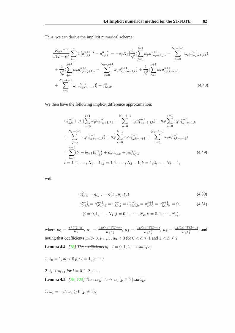
4.4 Implicit numerical method for the ST-FBTE 82
Thus, we can derive the implicit numerical scheme:
Kατ−α
Γ(2− α)
n∑
l=0
bl[un+1−li,j,k − un−l
i,j,k] = −cβKβ [1
hβx(i+1∑
p=0
ωpun+1i−p+1,j,k +
N1−i+1∑
p=0
ωpun+1i+p−1,j,k)
+1
hβy(
j+1∑
q=0
ωqun+1i,j−q+1,k +
N2−j+1∑
q=0
ωqun+1i,j+q−1,k) +
1
hβz(k+1∑
r=0
ωrun+1i,j,k−r+1
+
N3−k+1∑
r=0
ωrun+1i,j,k+r−1)] + fn
i,j,k. (4.48)
We then have the following implicit difference approximation:
un+1i,j,k + µ1(
i+1∑
p=0
ωpun+1i−p+1,j,k +
N1−i+1∑
p=0
ωpun+1i+p−1,j,k) + µ2(
j+1∑
q=0
ωqun+1i,j−q+1,k
+
N2−j+1∑
q=0
ωqun+1i,j+q−1,k) + µ3(
k+1∑
r=0
ωrun+1i,j,k−r+1 +
N3−k+1∑
r=0
ωrun+1i,j,k+r−1)
=n−1∑
l=0
(bl − bl+1)un−li,j,k + bnu
0i,j,k + µ0f
ni,j,k, (4.49)
i = 1, 2, · · · , N1 − 1, j = 1, 2, · · · , N2 − 1, k = 1, 2, · · · , N3 − 1,
with
u0i,j,k = gi,j,k = g(xi, yj, zk), (4.50)
un+10,j,k = un+1
N1,j,k= un+1
i,0,k = un+1i,N2,k
= un+1i,j,0 = un+1
i,j,N3= 0, (4.51)
(i = 0, 1, · · · , N1, j = 0, 1, · · · , N2, k = 0, 1, · · · , N3),
whereµ0 = ταΓ(2−α)Kα
, µ1 =cβKβτ
αΓ(2−α)
Kαhβx
, µ2 =cβKβτ
αΓ(2−α)
Kαhβy
, µ3 =cβKβτ
αΓ(2−α)
Kαhβz
, and
noting that coefficientsµ0 > 0, µ1, µ2, µ3 < 0 for 0 < α ≤ 1 and1 < β ≤ 2.
Lemma 4.4. [78] The coefficientsbl, l = 0, 1, 2, · · · satisfy:
1. b0 = 1, bl > 0 for l = 1, 2, · · · ;
2. bl > bl+1 for l = 0, 1, 2, · · · .
Lemma 4.5. [78, 123] The coefficientsωp (p ∈ N) satisfy:
1. ω1 = −β, ωp ≥ 0 (p 6= 1);

4.5 Stability of the implicit numerical method for the ST-FBTE 83
2.∞∑p=0
ωp = 0;
3. For any positive integern, we haven∑
p=0ωp < 0.
4.5 Stability of the implicit numerical method for the ST-FBTE
Let uni,j,k be the approximate solution of the INM (4.49)-(4.51), εni,j,k = uni,j,k − uni,j,k, and
En = [εn1,1,1, εn2,1,1, · · · , εnN1−1,N2−1,N3−1]
T .
Assuming‖En‖∞ = max1≤i≤N1−1,1≤j≤N2−1,1≤k≤N3−1
|εni,j,k|, and using mathematical induction,
we have the following theorem:
Theorem 4.1. The implicit numerical method defined by (4.49)-(4.51) is unconditionally
stable, and
‖En+1‖∞ ≤ ‖E0‖∞, n = 0, 1, 2, · · · . (4.52)
Proof. According to (4.49)-(4.51), the errorεni,j,k satisfies
εn+1i,j,k + µ1(
i+1∑
p=0
ωpεn+1i−p+1,j,k +
N1−i+1∑
p=0
ωpεn+1i+p−1,j,k) + µ2(
j+1∑
q=0
ωqεn+1i,j−q+1,k
+
N2−j+1∑
q=0
ωqεn+1i,j+q−1,k) + µ3(
k+1∑
r=0
ωrεn+1i,j,k−r+1 +
N3−k+1∑
r=0
ωrεn+1i,j,k+r−1)
=
n−1∑
m=0
(bm − bm+1)εn−mi,j,k + bnε
0i,j,k, (4.53)
(i = 1, 2, · · · , N1 − 1, j = 1, 2, · · · , N2 − 1, k = 1, 2, · · · , N3 − 1).
Whenn = 0, assume that‖E1‖∞ = max1≤i≤N1−1,1≤j≤N2−1,1≤k≤N3−1
|ε1i,j,k| = |ε1i∗,j∗,k∗|. Using

4.5 Stability of the implicit numerical method for the ST-FBTE 84
Lemmas4.4and4.5, and noting thatµ1, µ2, µ3 < 0, we have
‖E1‖∞ = |ε1i∗,j∗,k∗ |
≤ |ε1i∗,j∗,k∗ |+ µ1(i∗+1∑
p=0
ωp|ε1i∗,j∗,k∗ |+N1−i∗+1∑
p=0
ωp|ε1i∗,j∗,k∗|) + µ2(
j∗+1∑
q=0
ωq|ε1i∗,j∗,k∗|
+
N2−j∗+1∑
q=0
ωq|ε1i∗,j∗,k∗ |) + µ3(
k∗+1∑
r=0
ωr|ε1i∗,j∗,k∗ |+N3−k∗+1∑
r=0
ωr|ε1i∗,j∗,k∗|)
≤ |[1− 2β(µ1 + µ2 + µ3)]ε1i∗,j∗,k∗ + µ1(
i∗+1∑
p=0,p 6=1
ωpε1i∗−p+1,j∗,k∗
+
N1−i∗+1∑
p=0,p 6=1
ωpε1i∗+p−1,j∗,k∗) + µ2(
j∗+1∑
q=0,q 6=1
ωqε1i∗,j∗−q+1,k∗ +
N2−j∗+1∑
q=0,q 6=1
ωqε1i∗,j∗+q−1,k∗)
+µ3(
k∗+1∑
r=0,r 6=1
ωrε1i∗,j∗,k∗−r+1 +
N3−k∗+1∑
r=0,r 6=1
ωrε1i∗,j∗,k∗+r−1)|
= |ε1i∗,j∗,k∗ + µ1(i∗+1∑
p=0
ωpε1i∗−p+1,j∗,k∗ +
N1−i∗+1∑
p=0
ωpε1i∗+p−1,j∗,k∗) + µ2(
j∗+1∑
q=0
ωqε1i∗,j∗−q+1,k∗
+
N2−j∗+1∑
q=0
ωqε1i∗,j∗+q−1,k∗) + µ3(
k∗+1∑
r=0
ωrε1i∗,j∗,k∗−r+1 +
N3−k∗+1∑
r=0
ωrε1i∗,j∗,k∗+r−1)|
= b0|ε0i∗,j∗,k∗|
≤ ‖E0‖∞.
Now, suppose that‖Em‖∞ ≤ ‖E0‖∞,m = 1, 2, · · · , n. By assuming that‖En+1‖∞ =

4.6 Convergence of the implicit numerical method for the ST-FBTE 85
max1≤i≤N1−1,1≤j≤N2−1,1≤k≤N3−1
|εn+1i,j,k| = |εn+1
i∗,j∗,k∗|, using Lemmas4.4and4.5again, we obtain
‖En+1‖∞ = |εn+1i∗,j∗,k∗
|
≤ |εn+1i∗,j∗,k∗
|+ µ1(
i∗+1∑
p=0
ωp|εn+1i∗,j∗,k∗
|+N1−i∗+1∑
p=0
ωp|εn+1i∗,j∗,k∗
|) + µ2(
j∗+1∑
q=0
ωq|εn+1i∗,j∗,k∗
|
+
N2−j∗+1∑
q=0
ωq|εn+1i∗,j∗,k∗
|) + µ3(
k∗+1∑
r=0
ωr|εn+1i∗,j∗,k∗
|+N3−k∗+1∑
r=0
ωr|εn+1i∗,j∗,k∗
|)
≤ |[1− 2β(µ1 + µ2 + µ3)]εn+1i∗,j∗,k∗
+ µ1(
i∗+1∑
p=0,p 6=1
ωpεn+1i∗−p+1,j∗,k∗
+
N1−i∗+1∑
p=0,p 6=1
ωpεn+1i∗+p−1,j∗,k∗
) + µ2(
j∗+1∑
q=0,q 6=1
ωqεn+1i∗,j∗−q+1,k∗
+
N2−j∗+1∑
q=0,q 6=1
ωqεn+1i∗,j∗+q−1,k∗
)
+µ3(
k∗+1∑
r=0,r 6=1
ωrεn+1i∗,j∗,k∗−r+1 +
N3−k∗+1∑
r=0,r 6=1
ωrεn+1i∗,j∗,k∗+r−1)|
= |εn+1i∗,j∗,k∗
+ µ1(
i∗+1∑
p=0
ωpεn+1i∗−p+1,j∗,k∗
+
N1−i∗+1∑
p=0
ωpεn+1i∗+p−1,j∗,k∗
) + µ2(
j∗+1∑
q=0
ωqεn+1i∗,j∗−q+1,k∗
+
N2−j∗+1∑
q=0
ωqεn+1i∗,j∗+q−1,k∗
) + µ3(
k∗+1∑
r=0
ωrεn+1i∗,j∗,k∗−r+1 +
N3−k∗+1∑
r=0
ωrεn+1i∗,j∗,k∗+r−1)|
= |n−1∑
m=0
(bm − bm+1)εn−mi∗,j∗,k∗
+ bnε0i∗,j∗,k∗ |
≤n−1∑
m=0
(bm − bm+1)‖En−m‖∞ + bn‖E0‖∞
≤ (
n−1∑
m=0
(bm − bm+1) + bn)‖E0‖∞
= ‖E0‖∞.
Hence the implicit numerical method defined by (4.49)-(4.51) is unconditionally stable.
4.6 Convergence of the implicit numerical method for the ST-
FBTE
Settingeni,j,k = u(xi, yj , zk, tn)−uni,j,k, and we denoteRn = [en1,1,1, en2,1,1, · · · , enN1−1,N2−1,N3−1]
T ,
thenR0 = 0. HereRn and0 are((N1 − 1)× (N2 − 1)× (N3 − 1)) vectors, respectively.

4.6 Convergence of the implicit numerical method for the ST-FBTE 86
From (4.37)-(4.51), the erroreni,j,k satisfies
en+1i,j,k + µ1(
i+1∑
p=0
ωpen+1i−p+1,j,k +
N1−i+1∑
p=0
ωpen+1i+p−1,j,k) + µ2(
j+1∑
q=0
ωqen+1i,j−q+1,k
+
N2−j+1∑
q=0
ωqen+1i,j+q−1,k) + µ3(
k+1∑
r=0
ωren+1i,j,k−r+1 +
N3−k+1∑
r=0
ωren+1i,j,k+r−1)
=n−1∑
m=0
(bm − bm+1)en−mi,j,k + C1τ
α(τ2−α + hx + hy + hz), (4.54)
for i = 1, 2, · · · , N1 − 1, j = 1, 2, · · · , N2 − 1, k = 1, 2, · · · , N3 − 1.
Assuming ‖Rn+1‖∞ = max1≤i≤N1−1,1≤j≤N2−1,1≤k≤N3−1
|en+1i,j,k|, and using mathematical
induction, we have the following theorem:
Theorem 4.2. The implicit difference approximation defined by (4.49)-(4.51) is convergent,
and there is a positive constantC∗, such that
‖Rn+1‖∞ ≤ C∗(τ2−α + hx + hy + hz), n = 0, 1, 2, · · · . (4.55)
Proof. Whenn = 0, assume that‖R1‖∞ = max1≤i≤N1−1,1≤j≤N2−1,1≤k≤N3−1
|e1i,j,k| =
|e1i∗,j∗,k∗|. Using equation (4.54), Lemmas4.4and4.5, we have
‖R1‖∞ = |e1i∗,j∗,k∗|
≤ |e1i∗,j∗,k∗ |+ µ1(
i∗+1∑
p=0
ωp|e1i∗−p+1,j∗,k∗|+N1−i∗+1∑
p=0
ωp|e1i∗+p−1,j∗,k∗|)
+µ2(
j∗+1∑
q=0
ωq|e1i∗,j∗−q+1,k∗ |+N2−j∗+1∑
q=0
ωq|e1i∗,j∗+q−1,k∗|)
+µ3(
k∗+1∑
r=0
ωr|e1i∗,j∗,k∗−r+1|+N3−k∗+1∑
r=0
ωr|e1i∗,j∗,k∗+r−1|)
≤ |e1i∗,j∗,k∗ + µ1(
i∗+1∑
p=0
ωpe1i∗−p+1,j∗,k∗ +
N1−i∗+1∑
p=0
ωpe1i∗+p−1,j∗,k∗) + µ2(
j∗+1∑
q=0
ωqe1i∗,j∗−q+1,k∗
+
N2−j∗+1∑
q=0
ωqe1i∗,j∗+q−1,k∗) + µ3(
k∗+1∑
r=0
ωre1i∗,j∗,k∗−r+1 +
N3−k∗+1∑
r=0
ωre1i∗,j∗,k∗+r−1)|
= C1τα(τ2−α + hx + hy + hz)
= C1b−10 τα(τ2−α + hx + hy + hz).

4.7 Numerical results 87
Now, suppose that‖Rm‖∞ ≤ C1b−1m−1τ
α(τ2−α+hx+hy+hz),m = 1, 2, · · · , n. By assuming
that ‖Rn+1‖∞ = max1≤i≤N1−1,1≤j≤N2−1,1≤k≤N3−1
|en+1i,j,k | = |en+1
i∗,j∗,k∗|. Using Lemmas4.4 and
4.5, and equation (4.54) again, we have
‖Rn+1‖∞ = |en+1i∗,j∗,k∗
|
≤ |en+1i∗,j∗,k∗
|+ µ1(
i∗+1∑
p=0
ωp|en+1i∗−p+1,j∗,k∗
|+N1−i∗+1∑
p=0
ωp|en+1i∗+p−1,j∗,k∗
|)
+µ2(
j∗+1∑
q=0
ωq|en+1i∗,j∗−q+1,k∗
|+N2−j∗+1∑
q=0
ωq|en+1i∗,j∗+q−1,k∗
|) + µ3(
k∗+1∑
r=0
ωr|en+1i∗,j∗,k∗−r+1|
+
N3−k∗+1∑
r=0
ωr|en+1i∗,j∗,k∗+r−1|)
= |n−1∑
m=0
(bm − bm+1)en−mi∗,j∗,k∗
+ C1τα(τ2−α + hx + hy + hz)|
≤n−1∑
l=0
(bl − bl+1)C1b−1n−l−1τ
α(τ2−α + hx + hy + hz) + C1τα(τ2−α + hx + hy + hz)
≤n−1∑
l=0
(bl − bl+1)C1b−1n τα(τ2−α + hx + hy + hz) +C1τ
α(τ2−α + hx + hy + hz)
= C1b−1n τα(τ2−α + hx + hy + hz).
We note thatlimn→∞
b−1n
nα = limn→∞
n−α
(n+1)1−α−n1−α = 11−α , there exists a positive constantC2, such
that‖Rn+1‖∞ ≤ C1C2nατα(τ2−α + hx + hy + hz).
Finally, note thatnτ ≤ T is finite, so there exists a positive constantC∗, such that‖Rn+1‖∞ ≤
C∗(τ2−α + hx + hy + hz) for n = 0, 1, 2, · · · .
Hence the implicit numerical method defined by (4.49)-(4.51) is convergent.
4.7 Numerical results
Due to the complexity of the analytic solution given in this chapter, and the computational
overheads necessary to perform the simulations for NMR in three dimensions, we present here
a preliminary study based on a two-dimensional example to confirm our theoretical analysis.
Example 4.1. The following space and time fractional Bloch-Torrey equation with initial and
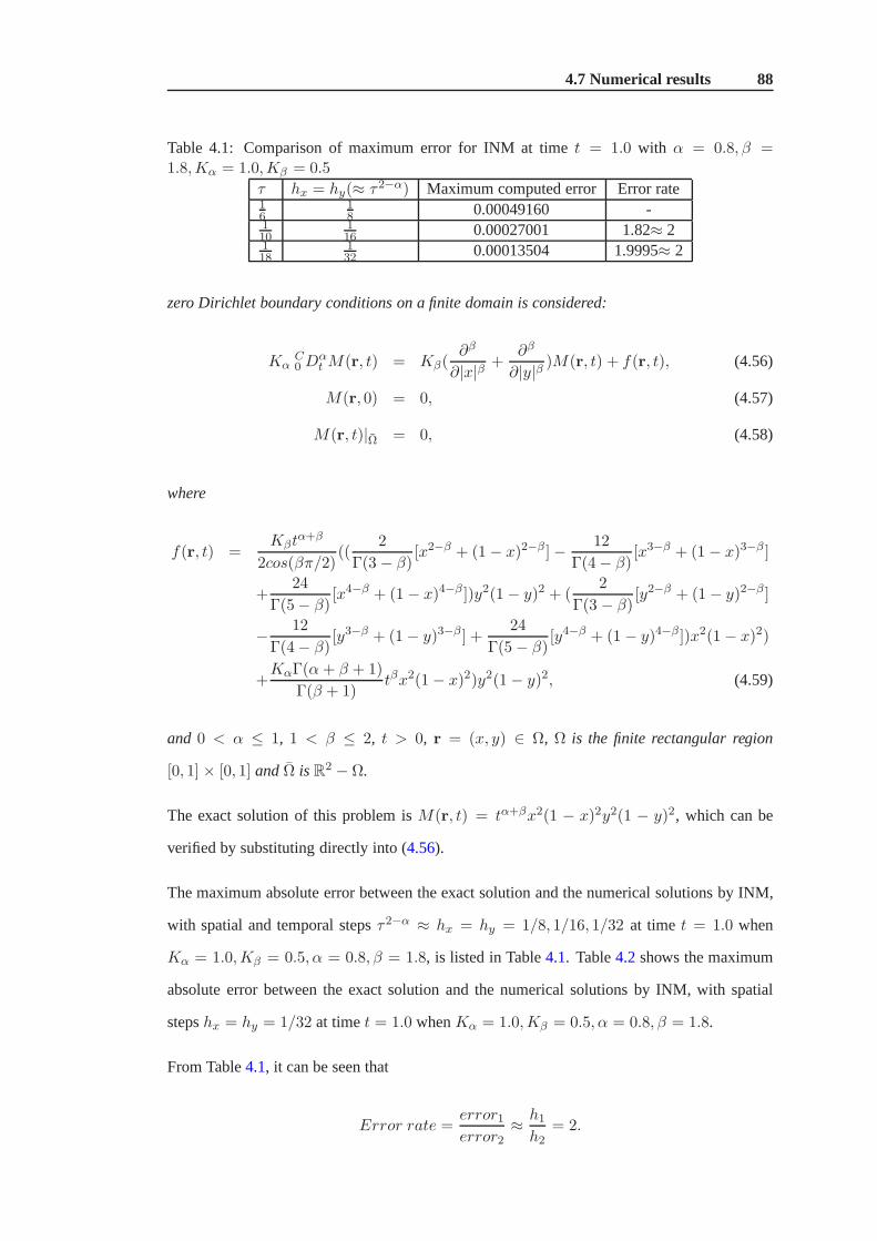
4.7 Numerical results 88
Table 4.1: Comparison of maximum error for INM at timet = 1.0 with α = 0.8, β =1.8,Kα = 1.0,Kβ = 0.5
τ hx = hy(≈ τ2−α) Maximum computed error Error rate16
18 0.00049160 -
110
116 0.00027001 1.82≈ 2
118
132 0.00013504 1.9995≈ 2
zero Dirichlet boundary conditions on a finite domain is considered:
KαC0 D
αt M(r, t) = Kβ(
∂β
∂|x|β +∂β
∂|y|β )M(r, t) + f(r, t), (4.56)
M(r, 0) = 0, (4.57)
M(r, t)|Ω = 0, (4.58)
where
f(r, t) =Kβt
α+β
2cos(βπ/2)((
2
Γ(3 − β)[x2−β + (1− x)2−β]− 12
Γ(4− β)[x3−β + (1− x)3−β ]
+24
Γ(5− β)[x4−β + (1− x)4−β ])y2(1− y)2 + (
2
Γ(3 − β)[y2−β + (1− y)2−β ]
− 12
Γ(4− β)[y3−β + (1− y)3−β ] +
24
Γ(5− β)[y4−β + (1− y)4−β])x2(1− x)2)
+KαΓ(α+ β + 1)
Γ(β + 1)tβx2(1− x)2)y2(1− y)2, (4.59)
and 0 < α ≤ 1, 1 < β ≤ 2, t > 0, r = (x, y) ∈ Ω, Ω is the finite rectangular region
[0, 1] × [0, 1] andΩ isR2 − Ω.
The exact solution of this problem isM(r, t) = tα+βx2(1 − x)2y2(1 − y)2, which can be
verified by substituting directly into (4.56).
The maximum absolute error between the exact solution and the numerical solutions by INM,
with spatial and temporal stepsτ2−α ≈ hx = hy = 1/8, 1/16, 1/32 at timet = 1.0 when
Kα = 1.0,Kβ = 0.5, α = 0.8, β = 1.8, is listed in Table4.1. Table4.2shows the maximum
absolute error between the exact solution and the numericalsolutions by INM, with spatial
stepshx = hy = 1/32 at timet = 1.0 whenKα = 1.0,Kβ = 0.5, α = 0.8, β = 1.8.
From Table4.1, it can be seen that
Error rate =error1error2
≈ h1h2
= 2.

4.7 Numerical results 89
Table 4.2: Comparison of maximum error for INM withhx = hy = 1/32 at timet = 1.0 whenα = 0.8, β = 1.8,Kα = 1.0,Kβ = 0.5
τ Maximum computed error Error rate14 0.00078984 -18 0.00035091 2.25≈ 2.30116 0.00015520 2.26≈ 2.30
From Table4.2, it can be seen that
Error rate =error1error2
≈ (τ1τ2)2−α = 2.3.
This is in good agreement with our theoretical analysis, namely that the convergence order of
the numerical method INM for this problem isO(τ2−α + hx + hy).
We now exhibit in Example4.2the result of INM for the space and time fractional Bloch-Torrey
equation with a nonlinear source term.
Example 4.2. Space and time fractional Bloch-Torrey equation with initial and zero Dirichlet
boundary conditions on a finite domain:
KαC0 D
αt M(r, t) = Kβ(
∂β
∂|x|β +∂β
∂|y|β )M(r, t) + f(M, r, t), (4.60)
M(r, 0) = δ(x− 0.5, y − 0.5), (4.61)
M(r, t)|Ω = 0, (4.62)
where the nonlinear source term is Fisher’s growth equationf(M, r, t) = 0.25M(r, t)[1 −
M(r, t)], and0 < α ≤ 1, 1 < β ≤ 2, t > 0, r = (x, y) ∈ Ω, Ω is the finite rectangular region
[0, 1] × [0, 1] andΩ isR2 − Ω.
The solution profiles of (4.60) by INM, with spatial and temporal stepshx = hy = 1/50,
τ = 1/26 at time t = 3/26 with Kα = 1.0, tfinal = 1.0 for different α, β andKβ are
listed in Figure4.1. From Figure4.1, it can be seen that the coefficientKβ impacts on the
solution profiles of (4.60), whereby a larger value ofKβ produces more diffuse profiles. In
Figure4.2, we illustrate the effect of the fractional order in space for this problem, with spatial
and temporal stepshx = hy = 1/50, τ = 1/26 at time t = 3/26 with Kα = 1.0,Kβ =
1.0, tfinal = 1.0 for β fixed at 2 andα varying. Here we can see that reducing the value of
α leads to a much sharper central peak. In Figure4.3, we illustrate the effect of the fractional

4.8 Conclusions 90
00.2
0.40.6
0.81
0
0.5
10
1
2
3
x 10−4
xy
M(x
,y,t
=3/2
6)
(a)
00.2
0.40.6
0.81
0
0.5
10
1
2
3
x 10−4
xy
M(x
,y,t
=3/2
6)
(b)
00.2
0.40.6
0.81
0
0.5
10
0.2
0.4
0.6
0.8
1
x 10−3
xy
M(x
,y,t
=3/2
6)
(c)
00.2
0.40.6
0.81
0
0.5
10
0.2
0.4
0.6
0.8
1
x 10−3
xy
M(x
,y,t
=3/2
6)
(d)
Figure 4.1: A plot of numerical solutions of ST-FBTE using the implicit numerical method(INM) with spatial and temporal stepshx = hy = 1/50, τ = 1/26 at time t = 3/26 withKα = 1.0, tfinal = 1.0 for differentα, β andKβ. (a) α = 1.0, β = 2.0,Kβ = 1.0. (b) α =1.0, β = 2.0,Kβ = 2.0. (c) α = 0.8, β = 1.8,Kβ = 1.0. (d) α = 0.8, β = 1.8,Kβ = 2.0.
order in time for this problem, with spatial and temporal stepshx = hy = 1/50, τ = 1/26 at
time t = 3/26 with Kα = 1.0,Kβ = 1.0, tfinal = 1.0 for α fixed at 1 andβ varying. Again
we see the peak sharping asβ is decreased. We observe where we now see that a much sharper
profile is obtained when we varyα with β fixed than when we varyβ with α fixed. Finally, the
effect of the fractional order in both time and space is illustrated in Figure4.4.
Overall, the coefficientKβ has a significant effect, especially for fractional values of α. The
most significant effects in terms of the spikiness of the profile occurs as bothα andβ are
simultaneously reduced.
4.8 Conclusions
In this chapter, an analytical solution and an effective implicit numerical method for solving the
fractional Bloch-Torrey equation in fractional Laplacianand Riesz forms, respectively, have

4.8 Conclusions 91
00.2
0.40.6
0.81
0
0.5
10
1
2
3
4
5
6
x 10−4
xy
M(x
,y,t
=3/2
6)
(a)
00.2
0.40.6
0.81
0
0.5
10
1
2
3
4
5
6
x 10−4
xy
M(x
,y,t
=3/2
6)
(b)
00.2
0.40.6
0.81
0
0.5
10
1
2
3
4
5
6
x 10−4
xy
M(x
,y,t
=3/2
6)
(c)
00.2
0.40.6
0.81
0
0.5
10
1
2
3
4
5
6
x 10−4
xy
M(x
,y,t
=3/2
6)
(d)
Figure 4.2: A plot of numerical solutions of ST-FBTE using the implicit numerical method(INM) with spatial and temporal stepshx = hy = 1/50, τ = 1/26 at time t = 3/26 withKα = 1.0,Kβ = 1.0, tfinal = 1.0 for β fixed at 2. (a) α = 1.0. (b) α = 0.9. (c) α = 0.8. (d)α = 0.6.
been derived. The stability and convergence of the implicitnumerical method are analysed
systematically. We have used our numerical method to simulate a problem of practical
importance involving a nonlinear source term. Our results have highlighted the impact of
the fractional indices on the shape of the solution profile. Finally, we note, however, that the
complexity of our solutions and the computational overheads of our methods are such that we
plan in the future to investigate alternate solution strategies for solving ST-FBTEs such as those
based on alternating direction implicit methods.

4.8 Conclusions 92
00.2
0.40.6
0.81
0
0.5
10
0.5
1
1.5
2
x 10−3
xy
M(x
,y,t
=3/2
6)
(a)
00.2
0.40.6
0.81
0
0.5
10
0.5
1
1.5
2
x 10−3
xy
M(x
,y,t
=3/2
6)
(b)
00.2
0.40.6
0.81
0
0.5
10
0.5
1
1.5
2
x 10−3
xy
M(x
,y,t
=3/2
6)
(c)
00.2
0.40.6
0.81
0
0.5
10
0.5
1
1.5
2
x 10−3
xy
M(x
,y,t
=3/2
6)
(d)
Figure 4.3: A plot of numerical solutions of ST-FBTE using the implicit numerical method(INM) with spatial and temporal stepshx = hy = 1/50, τ = 1/26 at time t = 3/26 withKα = 1.0,Kβ = 1.0, tfinal = 1.0 for α fixed at 1. (a) β = 2.0. (b) β = 1.8. (c) β = 1.6. (d)β = 1.2.

4.8 Conclusions 93
00.2
0.40.6
0.81
0
0.5
10
0.2
0.4
0.6
0.8
1
x 10−3
xy
M(x
,y,t
=3/2
6)
(a)
00.2
0.40.6
0.81
0
0.5
10
0.2
0.4
0.6
0.8
1
x 10−3
xy
M(x
,y,t
=3/2
6)
(b)
00.2
0.40.6
0.81
0
0.5
10
0.5
1
1.5
2
2.5
3
x 10−3
xy
M(x
,y,t
=3/2
6)
(c)
00.2
0.40.6
0.81
0
0.5
10
0.5
1
1.5
2
2.5
3
x 10−3
xy
M(x
,y,t
=3/2
6)
(d)
Figure 4.4: A plot of numerical solutions of ST-FBTE using the implicit numerical method(INM) with spatial and temporal stepshx = hy = 1/50, τ = 1/26 at time t = 3/26 withKα = 1.0,Kβ = 1.0, tfinal = 1.0 for different α and β. (a) α = 0.99, β = 1.9. (b)α = 0.8, β = 1.8. (c) α = 0.7, β = 1.5. (d) α = 0.5, β = 1.1.

CHAPTER 5
A computationally effective alternating direction
method for the space and time fractional Bloch-Torrey
equation in 3-D
5.1 Introduction
Recently, fractional order calculus has been used to examine the connection between fractional
order dynamics and diffusion to solve the Bloch-Torrey equation [14, 82, 83, 130, 141]. It
was pointed out that a fractional diffusion model could be successfully applied to analysing
diffusion images of human brain tissues and provide new insights into further investigations of
tissue structures and the microenvironment. Magin et al. [82] proposed a new diffusion model
for solving the Bloch-Torrey equation using fractional order calculus with respect to time and
space (ST-FBTE):
τα−1 C0 D
αt Mxy(r, t) = λMxy(r, t) +Dµ2(β−1)RβMxy(r, t), (5.1)

5.1 Introduction 95
whereλ = −iγ(r ·G(t)), r = (x, y, z), G(t) is the magnetic field gradient,γ andD are the
gyromagnetic ratio and the diffusion coefficient respectively. C0 D
αt is the Caputo-Djrbashian
time fractional derivative of orderα (0 < α ≤ 1) with respect tot, and with the starting point
at t = 0 is defined regularized as [4]:
C0 D
αt u(x, t) =
1
Γ(1− α)
[∂
∂t
∫ t
0
u(x, τ)
(t− τ)αdτ − u(x, 0)
tα
]. (5.2)
Rβ = (Rβx + Rβ
y + Rβz ) is a sequential Riesz fractional order operator in space [63];
Mxy(r, t) = Mx(r, t) + iMy(r, t), wherei =√−1, comprises the transverse components
of the magnetization; andτα−1 andµ2(β−1) are the fractional order time and space constants
needed to preserve units,(0 < α ≤ 1, and1 < β ≤ 2). Magin et al. [82] derived analytical
solutions with fractional order dynamics in space (i.e.,α = 1, β an arbitrary real number,
1 < β ≤ 2) and time (i.e.,0 < α < 1, andβ = 2), respectively. Yu et al. [141] derived an
analytical solution and an effective implicit numerical method for solving equation (5.1). They
also considered the stability and convergence properties of the implicit numerical method.
However, due to the computational overheads necessary to perform the simulations for ST-
FBTE in three dimensions, they presented a preliminary study based on a two-dimensional
example to confirm their theoretical analysis.
Alternating direction implicit (ADI) schemes have been proposed for the numerical simulations
of classic differential equations [34, 35, 107]. The ADI schemes reduce the multidimensional
problem into a series of independent one-dimensional problems and are thus computationally
efficient.
Since fractional derivatives are nonlocal and have historydependence, fractional problems
generally require a large amount of CPU time if traditional implicit schemes based on Gaussian
elimination are used. In order to overcome the computational difficulty, a number of authors
have applied ADI schemes for solving fractional problems. Meerschaert et al. [88] applied
a practical ADI method to solve a class of two-dimensional initial-boundary value space-
fractional partial differential equations with variable coefficients on a finite domain. They
proved that the ADI method is unconditionally stable and converges linearly. Chen and
Liu [26] used a new technique with a combination of the ADI-Euler method, the unshifted
Grunwald formula for the advection term, the right-shifted Grunwald formula for the diffusion

5.2 Preliminary knowledge 96
term, and Richardson extrapolation to establish an unconditionally stable second order accurate
difference method for a two-dimensional fractional advection-dispersion equation. Zhang and
Sun [152] used ADI schemes for a two-dimensional time-fractional sub-diffusion equation.
They proved the method is unconditionally stable and convergent by the discrete energy
method, and showed that the computational complexities andCPU time are reduced greatly.
Liu et al. [79] proposed a fractional ADI scheme for three-dimensional non-continued seepage
flow in uniform media and a modified Douglas scheme for the continued seepage flow in non-
uniform media. They proved that both methods are unconditionally stable and convergent.
In this chapter, we construct a fractional alternating direction method (FADM) for the three-
dimensional space and time fractional Bloch-Torrey equation (ST-FBTE) with initial and
boundary conditions on a finite domain, and prove that the FADM for the ST-FBTE is
unconditionally stable and convergent.
The structure of the remainder of this chapter is as follows.In Section5.2, some mathematical
preliminaries are introduced. In Section5.3, we propose a fractional alternating direction
method (FADM) for ST-FBTEs. The stability and consistency of the FADM are investigated in
Sections5.4and5.5, respectively. Finally, numerical results for ST-FBTEs are given to verify
our theoretical results.
5.2 Preliminary knowledge
In this section, we outline some preliminary knowledge usedthroughout the remaining sections
of this chapter. It is assumed throughout this section thatM(x, y, z, t) ∈ C3,3,3,2x,y,z,t (Ω) for
0 < α ≤ 1 and1 < β ≤ 2, wheret ∈ [0, T ] andΩ : −∞ ≤ x, y, z ≤ +∞.
Definition 5.1. LetM be as defined above on an infinite intervalΩ : −∞ ≤ x, y, z ≤ +∞.
The Riesz fractional operatorRβ is defined as [46]
RβxM(x, y, z, t) =
∂βM(x, y, z, t)
∂|x|β = −cβ(−∞Dβx +x D
β+∞)M(x, y, z, t), (5.3)

5.2 Preliminary knowledge 97
wherecβ = 1
2 cos(πβ2), β 6= 1,
−∞DβxM(x, y, z, t) =
1
Γ(2− β)
∂2
∂x2
∫ x
−∞
M(ξ, y, z, t)dξ(x− ξ)β−1
,
xDβ+∞M(x, y, z, t) =
(−1)2
Γ(2− β)
∂2
∂x2
∫ +∞
x
M(ξ, y, z, t)dξ(ξ − x)β−1
.
Similarly, we can define the Riesz fractional derivativesRβyM(x, y, z, t) = ∂βM(x,y,z,t)
∂|y|βand
RβzM(x, y, z, t) = ∂βM(x,y,z,t)
∂|z|βof orderβ (1 < β ≤ 2) with respect toy andz.
Lemma 5.1. Suppose thatM(x) ∈ C3(−∞,∞), the following equality holds
∂β
∂|x|βM(x) = − 1
2 cos πβ2
[−∞Dβx + xD
β+∞]M(x), (5.4)
where1 < β ≤ 2.
Proof. See [137, 158].
Lemma 5.2. Suppose thatM(x) ∈ C3[0, L], the following equality
∂β
∂|x|βM(x) = − 1
2 cos πβ2
[0Dβx + xD
βL]M
∗(x), (5.5)
also holds when setting
M∗(x) =
M(x), x ∈ (0, L),
0, x /∈ (0, L),
i.e.,M∗(x) = 0 on the boundary points and beyond the boundary points.
Proof. See [137, 158].
The use of Lemmas5.1 and5.2 above allows us to define the Riesz fractional operator on a
bounded setΩ with zero Dirichlet boundary conditions.
We present our solution techniques for solving the ST-FBTE in the following steps. Firstly, the
ST-FBTE (5.1) is rewritten in the form:
KαC0 D
αt Mxy(r, t) = λMxy(r, t) +KβRβMxy(r, t). (5.6)

5.3 Fractional alternating direction method 98
We equate real and imaginary components to express equation(5.6) as a coupled system of
partial differential equations for the componentsMx andMy, namely
KαC0 D
αt Mx(r, t) = λGMy(r, t) +Kβ(
∂β
∂|x|β +∂β
∂|y|β +∂β
∂|z|β )Mx(r, t), (5.7)
KαC0 D
αt My(r, t) = −λGMx(r, t) +Kβ(
∂β
∂|x|β +∂β
∂|y|β +∂β
∂|z|β )My(r, t), (5.8)
whereλG = γ(r ·G(t)).
For convenience, the ST-FBTEs (5.7) and (5.8) are decoupled (see [75]), which is equivalent
to solving a fractional in space and time partial differential equation of the form
KαC0 D
αt M(r, t) = Kβ(
∂β
∂|x|β +∂β
∂|y|β +∂β
∂|z|β )M(r, t) + f(r, t), (5.9)
whereM can be eitherMx or My, andf(r, t) = λGMy(r, t) if M = Mx, andf(r, t) =
−λGMx(r, t) if M = My.
5.3 Fractional alternating direction method
We propose a fractional alternating direction method for the space and time fractional Bloch-
Torrey equation (5.9) with initial and zero Dirichlet boundary conditions on a finite domain
given by
M(r, 0) = M0(r), (5.10)
M(r, t)|Ω = 0, (5.11)
where0 < α ≤ 1, 1 < β ≤ 2, 0 < t ≤ T , r = (x, y, z) ∈ Ω, Ω is the finite rectangular region
[0, L1]× [0, L2]× [0, L3], M0(r) = M0(x, y, z) is continuous onΩ, andΩ is R3 − Ω.
Suppose that the continuous problem (5.9)-(5.11) has a smooth solutionM(x, y, z, t) ∈
C3,3,3,2x,y,z,t (Ω). Let hx = L1/N1, hy = L2/N2, hz = L3/N3, andτ = T/N be the spatial
and time steps, respectively. At a point(xi, yj , zk) at the moment of timetn for i, j, k ∈ N
andn ∈ N, we denote the exact and numerical solutionsM(r, t) asu(xi, yj, zk, tn) anduni,j,k,
respectively.

5.3 Fractional alternating direction method 99
Firstly, adopting the scheme in [123], we discretize the Caputo-Djrbashian time fractional
derivative ofu(xi, yj, zk, tn+1) as
C0 D
αt u(xi, yj, zk, t)|t=tn+1
=τ−α
Γ(2− α)
n∑
l=0
bl[u(xi, yj, zk, tn+1−l)− u(xi, yj , zk, tn−l)] +O(τ2−α), (5.12)
wherebl = (l + 1)1−α − l1−α, l = 0, 1, · · · , N .
Using the relationship between the Riemann-Liouville derivative and the Grunwald-Letnikov
scheme, we discretize the Riesz fractional derivative by the shifted Grunwald-Letnikov scheme
[137]
0Dβxu(x, yj , zk, tn+1)|x=xi
=1
hβx
i+1∑
p=0
ωpu(xi−p+1, yj , zk, tn+1) +O(hx), (5.13)
xDβL1u(x, yj , zk, tn+1)|x=xi
=1
hβx
N1−i+1∑
p=0
ωpu(xi+p−1, yj, zk, tn+1) +O(hx),(5.14)
where the coefficients are defined by
ω0 = 1, ωp = (−1)pβ(β − 1) · · · (β − p+ 1)
p!, p = 1, 2, · · · , N1. (5.15)
Similar results hold for the fractionaly andz derivatives.
Thus, we can derive the implicit numerical scheme:
Kατ−α
Γ(2− α)
n∑
l=0
bl[un+1−li,j,k − un−l
i,j,k] = −cβKβ [1
hβx(
i+1∑
p=0
ωpun+1i−p+1,j,k +
N1−i+1∑
p=0
ωpun+1i+p−1,j,k)
+1
hβy(
j+1∑
q=0
ωqun+1i,j−q+1,k +
N2−j+1∑
q=0
ωqun+1i,j+q−1,k) +
1
hβz(
k+1∑
r=0
ωrun+1i,j,k−r+1
+
N3−k+1∑
r=0
ωrun+1i,j,k+r−1)] + fn+1
i,j,k . (5.16)

5.3 Fractional alternating direction method 100
Rearranging (5.16), we then have the following implicit difference approximation:
un+1i,j,k + µ1(
i+1∑
p=0
ωpun+1i−p+1,j,k +
N1−i+1∑
p=0
ωpun+1i+p−1,j,k) + µ2(
j+1∑
q=0
ωqun+1i,j−q+1,k
+
N2−j+1∑
q=0
ωqun+1i,j+q−1,k) + µ3(
k+1∑
r=0
ωrun+1i,j,k−r+1 +
N3−k+1∑
r=0
ωrun+1i,j,k+r−1)
=n−1∑
l=0
(bl − bl+1)un−li,j,k + bnu
0i,j,k + µ0f
n+1i,j,k , (5.17)
i = 1, 2, · · · , N1 − 1, j = 1, 2, · · · , N2 − 1, k = 1, 2, · · · , N3 − 1,
with
u0i,j,k = gi,j,k = g(xi, yj, zk),
un+10,j,k = un+1
N1,j,k= un+1
i,0,k = un+1i,N2,k
= un+1i,j,0 = un+1
i,j,N3= 0,
(i = 0, 1, · · · , N1, j = 0, 1, · · · , N2, k = 0, 1, · · · , N3),
whereµ0 = ταΓ(2−α)Kα
, µ1 =cβKβτ
αΓ(2−α)
Kαhβx
, µ2 =cβKβτ
αΓ(2−α)
Kαhβy
, µ3 =cβKβτ
αΓ(2−α)
Kαhβz
, and
noting that coefficientsµ0 > 0, µ1, µ2, µ3 < 0 for 0 < α ≤ 1 and1 < β ≤ 2.
Lemma 5.3. [78] The coefficientsbl, l = 0, 1, 2, · · · satisfy:
1. b0 = 1, bl > 0 for l = 1, 2, · · · ;
2. bl > bl+1 for l = 0, 1, 2, · · · .
Lemma 5.4. [78, 123] The coefficientsωp (p ∈ N) satisfy:
1. ω1 = −β, ωp ≥ 0 (p 6= 1);
2.∞∑p=0
ωp = 0;
3. For any positive integern, we haven∑
p=0ωp < 0.
We consider the following fractional partial differentialdiscrete operator:
δβxun+1i,j,k =
i+1∑
p=0
ωpun+1i−p+1,j,k +
N1−i+1∑
p=0
ωpun+1i+p−1,j,k, (5.18)
which is anO(hx) approximation of the Riesz fractional derivative by the shifted Grunwald-
Letnikov scheme (5.13) and (5.14) [137]. Similarly, the following fractional partial differential

5.3 Fractional alternating direction method 101
discrete operators:
δβy un+1i,j,k =
j+1∑
q=0
ωqun+1i,j−q+1,k +
N2−j+1∑
q=0
ωqun+1i,j+q−1,k, (5.19)
δβz un+1i,j,k =
k+1∑
r=0
ωrun+1i,j,k−r+1 +
N3−k+1∑
r=0
ωrun+1i,j,k+r−1, (5.20)
areO(hy) andO(hz) approximation of the Riesz fractional derivatives, respectively.
Thus, the implicit difference scheme (5.17) may be rearranged in the following form involving
δβx , δβy andδβz :
(1 + µ1δβx + µ2δ
βy + µ3δ
βz )u
n+1i,j,k =
n−1∑
l=0
(bl − bl+1)un−li,j,k + bnu
0i,j,k + µ0f
n+1i,j,k . (5.21)
The implicit difference scheme (5.17) for the ST-FBTE has a local truncation error of the form
O(τ2−α+hx+hy+hz) and is unconditionally stable (refer to the proof of Theorem5.1in this
chapter). Unfortunately, (5.17) provides us with a linear system of equations for calculating
the difference solutionun+1i,j,k, that does not have the good property of the coefficient matrix
being banded but still has a regular sparse structure in thatall the off diagonal blocks are
themselves diagonal matrices. However, this can complicate the solution of the corresponding
linear system of equations.
Therefore, we adopt the alternating direction implicit method used in [79]. Our aim is to divide
the calculation into three steps with reduced calculation.In the first step, we solve the problem
in thex-direction, in the second step, we solve the problem in they-direction, finally in the
third step we solve the problem in thez-direction. For example, we introduce an additional
negligible term (see Theorem5.2)
(µ1µ2δβxδ
βy + µ1µ3δ
βxδ
βz + µ2µ3δ
βy δ
βz + µ1µ2µ3δ
βxδ
βy δ
βz )u
n+1i,j,k (5.22)
to the left side of (5.21) that has no impact on the convergence of the scheme to obtain
(1 + µ1δβx )(1 + µ2δ
βy )(1 + µ3δ
βz )u
n+1i,j,k =
n−1∑
l=0
(bl − bl+1)un−li,j,k + bnu
0i,j,k + µ0f
n+1i,j,k . (5.23)

5.3 Fractional alternating direction method 102
Hence, the FADM at timetn+1 is defined as:
(1 + µ1δβx )u
n+1/3i,j,k =
n−1∑
l=0
(bl − bl+1)un−li,j,k + bnu
0i,j,k + µ0f
n+1i,j,k , (5.24)
(1 + µ2δβy )u
n+2/3i,j,k = u
n+1/3i,j,k , (5.25)
(1 + µ3δβz )u
n+1i,j,k = u
n+2/3i,j,k . (5.26)
Together with the boundary valuesun+1/30,j,k andun+1/3
N1,j,kcalculated below, the coefficient matrix
Aj,k = (aj,k)s,t of the linear system (5.24) can be obtained as follows: for each fixed(j, k),
(aj,k)s,t =
µ1ωt−s+1, t ≥ s+ 2, s = 1, 2, · · · , N1 − 3,
µ1(ω0 + ω2), t = s+ 1, s = 1, 2, · · · , N1 − 2,
1 + 2µ1ω1, t = s = 1, 2, · · · , N1 − 1,
µ1(ω0 + ω2), t = s− 1, s = 2, · · · , N1 − 1,
µ1ωs−t+1, t ≤ s− 2, s = 3, 4, · · · , N1 − 1.
(5.27)
The coefficient matricesBi,k = (bi,k)s,t andCi,j = (ci,j)s,t can be shown to have similar form
to the matrixAj,k.
Similar to the alternating direction method for the classical integer-order PDE, in order to
maintain the approximation order, it is necessary to provide the additional boundary values in
thex-directionun+1/30,j,k , u
n+1/3N1,j,k
and in they-directionun+2/3i,0,k , u
n+2/3i,N2,k
, when solving the system
of equations with coefficient matricesAj,k andBi,k. For example, we provide the additional
boundary valuesun+1/30,j,k , u
n+1/3N1,j,k
according to:
un+1/3i,j,k = (1 + µ2δ
βy )(1 + µ3δ
βz )u
n+1i,j,k, i = 0, N1, (5.28)
wherej = 1, · · · , N2 − 1, k = 1, · · · , N3 − 1, n = 0, 1, · · · , N − 1, andun+2/3i,0,k , u
n+2/3i,N2,k
can
be obtained from
un+2/3i,j,k = (1 + µ3δ
βz )u
n+1i,j,k, j = 0, N2, (5.29)
wherei = 1, · · · , N1 − 1, k = 1, · · · , N3 − 1, n = 0, 1, · · · , N − 1.
From the three coefficient matrices, it can be seen that at each time step, we must solve, for each
fixed (j, k) (every layer in thex-direction) or each fixed(i, k) (every layer in they-direction)

5.4 Stability of FADM 103
or each fixed(i, j) (every layer in thez-direction) a linear system of equations withN1 − 1, or
N2 − 1, orN3 − 1 unknowns.
5.4 Stability of FADM
LetX = [x1, x2, · · · , xm]T ∈ Rm, ‖X‖∞ = max
1≤i≤m|xi|.
Lemma 5.5. Let the matrixD = (di,j)m×m ∈ Rm×m satisfy the conditions
m∑l=1,l 6=i
|di,l| ≤
|di,i| − 1, (i = 1, 2, · · · ,m), then
‖X‖∞ ≤ ‖DX‖∞. (5.30)
Proof. See [27].
In order to prove the stability of FADM, we need to rewrite (5.23)-(5.26) in matrix form.
Utilizing (5.27), the linear system (5.24) may be written in matrix form as
Aj,kUn+1/3j,k =
n−1∑
l=0
(bl − bl+1)Un−lj,k + bnU
0j,k + µ0F
n+1j,k + (0, · · · , 0, µ1u
n+1/3N1,j,k
)T , (5.31)
where1 ≤ j ≤ N2 − 1, 1 ≤ k ≤ N3 − 1, Un+1/3j,k = (u
n+1/31,j,k , u
n+1/32,j,k , · · · , un+1/3
N1−1,j,k)T ,
Aj,k = (aj,k)s,t, andFn+1j,k = (fn+1
1,j,k, fn+12,j,k, · · · , fn+1
N1−1,j,k)T .
Similarly, (5.25) may be written in matrix form as
Bi,kUn+2/3i,k = U
n+1/3i,k + (0, · · · , 0, µ2u
n+2/3i,N2,k
)T , (5.32)
where1 ≤ i ≤ N1 − 1, 1 ≤ k ≤ N3 − 1, Un+2/3i,k = (u
n+2/3i,1,k , u
n+2/3i,2,k , · · · , un+2/3
i,N2−1,k)T ,
Bi,k = (bi,k)s,t, andUn+1/3i,k = (u
n+1/3i,1,k , u
n+1/3i,2,k , · · · , un+1/3
i,N2−1,k)T .
(5.26) may be written in matrix form as
Ci,jUn+1i,j = U
n+2/3i,j + (0, · · · , 0, µ3u
n+1i,j,N3
)T , (5.33)
where1 ≤ i ≤ N1 − 1, 1 ≤ j ≤ N2 − 1, Un+1i,j = (un+1
i,j,1 , un+1i,j,2 , · · · , un+1
i,j,N3−1)T , Ci,j =

5.4 Stability of FADM 104
(ci,j)s,t, andUn+2/3i,j = (u
n+2/3i,j,1 , u
n+2/3i,j,2 , · · · , un+2/3
i,j,N3−1)T .
Thus, (5.23) may be written in matrix form as
STV Un+1 =
n−1∑
l=0
(bl − bl+1)Un−l + bnU
0 +Rn+1∗ , (5.34)
whereUn+1 is appropriately ordered.
The matricesS, T andV represent the operators(1 + µ1δβx ), (1 + µ2δ
βy ) and (1 + µ3δ
βz ),
respectively, and the vectorRn+1∗ comprises the source term and the boundary conditions in
the discretized equation.
Let uni,j,k be the approximate solution of (5.23). Settingεni,j,k = uni,j,k − uni,j,k, denoting
εn = (εn1,1,1, εn2,1,1, · · · , εnN1−1,N2−1,N3−1)
T ,
then the error satisfies
STV εn+1 =n−1∑
l=0
(bl − bl+1)εn−l + bnε
0. (5.35)
Thus, using mathematical induction, we have the following result:
Theorem 5.1. The FADM defined by (5.23) is unconditionally stable, and
‖εn+1‖∞ ≤ ‖ε0‖∞, n = 0, 1, 2, · · · .
Proof. From Lemma5.4, it can be seen thatAj,k, Bi,k andCi,j satisfy the condition of Lemma
5.5. According to the relationship between the matricesS andAj,k, T andBi,k, andV and
Ci,j, we see thatS, T andV also satisfy the condition of Lemma5.5. Therefore, whenn = 0,
using Lemmas5.3and5.5, we have
‖ε1‖∞ ≤ ‖V ε1‖∞ ≤ ‖TV ε1‖∞ ≤ ‖STV ε1‖∞ = ‖b0ε0‖∞ = ‖ε0‖∞.
Now, suppose that‖εm‖∞ ≤ ‖ε0‖∞, m = 1, 2, · · · , n. Similarly, using Lemmas5.3 and5.5

5.5 Consistency of FADM 105
again, we have
‖εn+1‖∞ ≤ ‖V εn+1‖∞ ≤ ‖TV εn+1‖∞ ≤ ‖STV εn+1‖∞
=
∥∥∥∥∥
n−1∑
l=0
(bl − bl+1)εn−l + bnε
0
∥∥∥∥∥∞
≤n−1∑
l=0
(bl − bl+1)‖εn−l‖∞ + bn‖ε0‖∞
≤(
n−1∑
l=0
(bl − bl+1) + bn
)‖ε0‖∞
= ‖ε0‖∞.
Hence the FADM defined by (5.23) is unconditionally stable.
5.5 Consistency of FADM
To obtain the consistency of the FADM, we note that the time difference operator in (5.21) has a
local truncation error of orderO(τ2−α), and the three space difference operators in (5.21) have
local truncation errors of ordersO(hx), O(hy) andO(hz), respectively, which was proved in
[141]. The only remaining term in the local error of the FADM is theadditional small term
(5.22).
For any positive integerl, let W l,1(R3) denote the collection of all functionsf ∈ C l(R3)
whose partial derivatives up to orderl are inL1(R3) and whose partial derivatives up to order
l − 1 vanish at infinity [88].
From Definition5.1, we have
∂β
∂|x|β∂β
∂|y|β u(x, y, z, t) = c2β(0Dβx +x D
βL1)(0D
βy +y D
βL2)u(x, y, z, t)
= c2β(0Dβx 0D
βy +0 D
βx yD
βL2
+x DβL1 0D
βy +x D
βL1 yD
βL2)u(x, y, z, t), (5.36)
Let r > 2β + 3 be an integer, and integersp, q ≥ 0, then forf ∈ W l,1(R3), we have (see

5.5 Consistency of FADM 106
Theorem 3.1 in [88])
h−βx h−β
y
∞∑
n=0
∞∑
m=0
ωnωmu(x− (n− p)hx, y − (m− q)hy, z, t)
=0 Dβx 0D
βyu(x, y, z, t) +O(hx + hy) (5.37)
uniformly in (x, y, z) ∈ R3.
Now firstly we discuss the additional perturbation errorµ1µ2δβxδ
βy u
n+1i,j,k. From (5.18) and
(5.19), we have
δβxδβy u
n+1i,j,k = δβx
j+1∑
q=0
ωqun+1i,j−q+1,k +
N2−j+1∑
q=0
ωqun+1i,j+q−1,k
=
j+1∑
q=0
ωq
i+1∑
p=0
ωpun+1i−p+1,j−q+1,k +
N1−i+1∑
p=0
ωpun+1i+p−1,j−q+1,k
+
N2−j+1∑
q=0
ωq
i+1∑
p=0
ωpun+1i−p+1,j+q−1,k +
N1−i+1∑
p=0
ωpun+1i+p−1,j+q−1,k
=
i+1∑
p=0
j+1∑
q=0
ωpωqun+1i−p+1,j−q+1,k +
N1−i+1∑
p=0
j+1∑
q=0
ωpωqun+1i+p−1,j−q+1,k
+i+1∑
p=0
N2−j+1∑
q=0
ωpωqun+1i−p+1,j+q−1,k +
N1−i+1∑
p=0
N2−j+1∑
q=0
ωpωqun+1i+p−1,j+q−1,k. (5.38)
With boundary condition (5.11), the solution function may be zero-extending forx < 0 or
y < 0. According to (5.37), we have
h−βx h−β
y
i+1∑
p=0
j+1∑
q=0
ωpωqun+1i−p+1,j−q+1,k = h−β
x h−βy
∞∑
p=0
∞∑
q=0
ωpωqun+1i−p+1,j−q+1,k
=0 Dβx 0D
βyu(xi, yj , zk, tn+1) +O(hx + hy). (5.39)
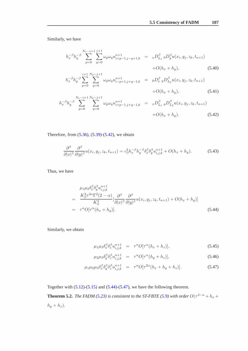
5.5 Consistency of FADM 107
Similarly, we have
h−βx h−β
y
N1−i+1∑
p=0
j+1∑
q=0
ωpωqun+1i+p−1,j−q+1,k = xD
βL1 0D
βyu(xi, yj, zk, tn+1)
+O(hx + hy), (5.40)
h−βx h−β
y
i+1∑
p=0
N2−j+1∑
q=0
ωpωqun+1i−p+1,j+q−1,k = 0D
βx yD
βL2u(xi, yj , zk, tn+1)
+O(hx + hy), (5.41)
h−βx h−β
y
N1−i+1∑
p=0
N2−j+1∑
q=0
ωpωqun+1i+p−1,j+q−1,k = xD
βL1 yD
βL2u(xi, yj, zk, tn+1)
+O(hx + hy). (5.42)
Therefore, from (5.36), (5.39)-(5.42), we obtain
∂β
∂|x|β∂β
∂|y|β u(xi, yj , zk, tn+1) = c2βh−βx h−β
y δβxδβy u
n+1i,j,k +O(hx + hy). (5.43)
Thus, we have
µ1µ2δβxδ
βy u
n+1i,j,k
=K2
βτ2αΓ2(2− α)
K2α
[∂β
∂|x|β∂β
∂|y|β u(xi, yj , zk, tn+1) +O(hx + hy)]
= ταO[τα(hx + hy)]. (5.44)
Similarly, we obtain
µ1µ3δβxδ
βz u
n+1i,j,k = ταO[τα(hx + hz)], (5.45)
µ2µ3δβy δ
βz u
n+1i,j,k = ταO[τα(hy + hz)], (5.46)
µ1µ2µ3δβxδ
βy δ
βz u
n+1i,j,k = ταO[τ2α(hx + hy + hz)]. (5.47)
Together with (5.12)-(5.15) and (5.44)-(5.47), we have the following theorem.
Theorem 5.2. The FADM (5.23) is consistent to the ST-FBTE (5.9) with orderO(τ2−α+hx+
hy + hz).

5.5 Consistency of FADM 108
Settingeni,j,k = u(xi, yj, zk, tn)− uni,j,k, and let
en = (en1,1,1, en2,1,1, · · · , enN1−1,N2−1,N3−1)
T ,
thene0 = 0.
From (5.12)-(5.15) and (5.44)-(5.47), the erroren satisfies
STV en+1 =
n−1∑
l=0
(bl − bl+1)en−l + C1τ
α(τ2−α + hx + hy + hz). (5.48)
Thus, using mathematical induction, we have the following result:
Theorem 5.3. The FADM (5.23) is convergent, and there is a positive constantC∗, such that
‖en+1‖∞ ≤ C∗(τ2−α + hx + hy + hz). (5.49)
Proof. Whenn = 0, and using Lemmas5.3, 5.4and5.5, we have
‖e1‖∞ ≤ ‖V e1‖∞ ≤ ‖TV e1‖∞ ≤ ‖STV e1‖∞ = C1τα(τ2−α + hx + hy + hz).
Now, suppose that
‖em‖∞ ≤ C1b−1m−1τ
α(τ2−α + hx + hy + hz),
wherem = 1, 2, · · · , n. Using Lemmas5.3, 5.4and5.5again, we have
‖en+1‖∞ ≤ ‖V en+1‖∞ ≤ ‖TV en+1‖∞ ≤ ‖STV en+1‖∞
= ‖n−1∑
l=0
(bl − bl+1)en−l + C1τ
α(τ2−α + hx + hy + hz)‖∞
≤n−1∑
l=0
(bl − bl+1)C1b−1n−l−1τ
α(τ2−α + hx + hy + hz) + C1τα(τ2−α + hx + hy + hz)
≤n−1∑
l=0
(bl − bl+1)C1b−1n τα(τ2−α + hx + hy + hz) +C1τ
α(τ2−α + hx + hy + hz)
= C1b−1n τα(τ2−α + hx + hy + hz).

5.6 Numerical results 109
We note that
limn→∞
b−1n
nα= lim
n→∞
n−α
(n+ 1)1−α − n1−α=
1
1− α,
and there exists a positive constantC2, such that
‖en+1‖∞ ≤ C1C2nατα(τ2−α + hx + hy + hz).
Finally, note thatnτ ≤ T is finite, so there exists a positive constantC∗, such that‖en+1‖∞ ≤
C∗(τ2−α + hx + hy + hz) for n = 0, 1, 2, · · · .
Hence the FADM (5.23) is convergent.
5.6 Numerical results
In order to better present the efficiency of the fractional alternating direction method, we first
show a two-dimensional example to confirm our theoretical analysis. The machine we used to
perform the numerical tests in this section is a laptop Lenovo Y430.
In Example5.1, we use the same example in [141] for comparison.
Example 5.1. The following space and time fractional Bloch-Torrey equation with initial and
zero Dirichlet boundary conditions on a finite domain is considered (See [141]):
KαC0 D
αt M(r, t) = Kβ(
∂β
∂|x|β +∂β
∂|y|β )M(r, t) + f(r, t), (5.50)
M(r, 0) = 0, (5.51)
M(r, t)|Ω = 0, (5.52)
where
f(r, t) =Kβt
α+β
2cos(βπ/2)
(
2
Γ(3− β)[x2−β + (1− x)2−β]− 12
Γ(4− β)[x3−β + (1− x)3−β]
+24
Γ(5− β)[x4−β + (1− x)4−β ])y2(1− y)2 + (
2
Γ(3− β)[y2−β + (1− y)2−β]
− 12
Γ(4− β)[y3−β + (1− y)3−β ] +
24
Γ(5− β)[y4−β + (1− y)4−β])x2(1− x)2
+KαΓ(α+ β + 1)
Γ(β + 1)tβx2(1− x)2)y2(1− y)2,

5.6 Numerical results 110
Table 5.1: Comparison of CPU time (seconds) between 2D-FADM, M1 and M2 with temporalstepτ = 1/100 at timet = 1.0
hx = hy 2D-FADMM1 M2
G-E J G-S G-E J G-S18 0.15 5.52 3.86 3.19 4.17 3.38 2.39116 0.32 28.06 12.77 11.90 23.58 12.50 12.34132 2.58 1356.33 63.05 59.34 1370.75 61.38 58.56
and 0 < α ≤ 1, 1 < β ≤ 2, t > 0, r = (x, y) ∈ Ω, Ω is the finite rectangular region
[0, 1] × [0, 1], andΩ isR2 − Ω.
The exact solution of this problem isM(r, t) = tα+βx2(1 − x)2y2(1 − y)2, which can be
verified by substituting directly into (5.50).
We takeKα = 1.0,Kβ = 0.5, α = 0.8, andβ = 1.8. Table5.1 lists the CPU time calculated
by a two-dimensional fractional alternating direction method (2D-FADM), a two-dimensional
implicit numerical scheme (M1) [141] that is first order accuracy in space, and a two-
dimensional implicit numerical method (M2) [125] that is second order accuracy in space at
timet = 1.0, where the temporal stepτ = 1/100 and spatial stepshx = hy = 1/8, 1/16, 1/32.
In Table5.1, G-E, J and G-S signify the use of Gauss elimination, Jacobi iteration and Gauss-
Seidel iteration for M1 or M2, respectively. A brief description of 2D-FADM, M1 and M2 is
presented in the Appendix5.8.
From Table5.1, it can be seen that the use of direct methods to solve the traditional
implicit numerical schemes for these fractional-in-spacemodels are extremely time-consuming
compared with using indirect methods. In fact there is a morethan 20 fold reduction in
computing time when the Gauss-Seidel method is employed forthe smaller mesh size of
hx = hy = 1/32. One notes that even though the fractional alternating direction method
requires the solution of smaller dense matrices of much reduced dimension using direct
methods at each cycle, it is still more computationally efficient than these classical iterative
strategies, with greatly reduced CPU time for all mesh sizes. In particular, the reduction in
CPU time for the FADM is even more significant for smaller meshsizes. One observes for
the smaller meshhx = hy = 1/32 a 20 fold reduction in CPU time over the Gauss-Seidel
method. The fractional alternating direction method is clearly the most efficient of the methods
investigated here for solving the large fractional-in-space linear systems.

5.6 Numerical results 111
We now exhibit in Example5.2 the application of FADM on the space and time fractional
Bloch-Torrey equation in 3-D with initial and boundary conditions on a finite domain.
Example 5.2. The following space and time fractional Bloch-Torrey equation in 3-D with
initial and zero Dirichlet boundary conditions on a finite domain is considered:
KαC0 D
αt M(r, t) = Kβ(
∂β
∂|x|β +∂β
∂|y|β +∂β
∂|z|β )M(r, t) + f(r, t), (5.53)
M(r, 0) = 0, (5.54)
M(r, t)|Ω = 0, (5.55)
where
f(r, t) =Kβt
α+β
2cos(βπ/2)
(
2
Γ(3− β)[x2−β + (1− x)2−β]− 12
Γ(4− β)[x3−β + (1− x)3−β]
+24
Γ(5− β)[x4−β + (1− x)4−β ])y2(1− y)2z2(1− z)2
+(2
Γ(3− β)[y2−β + (1− y)2−β]− 12
Γ(4− β)[y3−β + (1− y)3−β ]
+24
Γ(5− β)[y4−β + (1− y)4−β ])x2(1− x)2z2(1− z)2
+(2
Γ(3− β)[z2−β + (1− z)2−β ]− 12
Γ(4− β)[z3−β + (1− z)3−β ]
+24
Γ(5− β)[z4−β + (1− z)4−β ])x2(1− x)2y2(1− y)2
+KαΓ(α+ β + 1)
Γ(β + 1)tβx2(1− x)2y2(1− y)2z2(1− z)2,
and0 < α ≤ 1, 1 < β ≤ 2, t > 0, r = (x, y, z) ∈ Ω,Ω is the finite region[0, 1]×[0, 1]×[0, 1],
andΩ is R3 − Ω.
The exact solution of this problem isM(r, t) = tα+βx2(1 − x)2y2(1− y)2z2(1 − z)2, which
can be verified by substituting directly into (5.53).
In Example5.2, we takeKα = 1.0,Kβ = 0.5, α = 0.8, andβ = 1.8. The fractional
alternating direction implicit scheme, which is presentedin Section5.3, is used to solve this
problem. Table5.2 lists the CPU time and the maximum absolute error between theexact
solution and the numerical solutions obtained by FADM at time t = 1.0, where the temporal
stepτ = 1/100 and spatial stepshx = hy = hz = 1/4, 1/8, 1/16, 1/32.
From Table5.2, it can be seen that for the same spatial step, the FADM is convergent, which

5.6 Numerical results 112
Table 5.2: Comparison of CPU time and maximum error for FADM with temporal stepτ =1/100 at timet = 1.0
hx = hy = hz Maximum error CPU time(seconds)14 0.003750 0.1218 0.001267 0.55116 0.0003537 6.63132 0.0001675 121.29
is consistent with our theoretical findings. We also note that although the 3D-INS implicit
scheme could not be run on the laptop Lenovo Y430 due to its memory requirements, FADM
was successful. However, this method still required considerable CPU time to obtain the 3-D
solution.
We now exhibit in Example5.3 the result of FADM for the space and time fractional Bloch-
Torrey equation with a cubic nonlinear source term.
Example 5.3. The following space and time fractional Bloch-Torrey equation in 3-D with
initial and zero Dirichlet boundary conditions on a finite domain is considered:
KαC0 D
αt M(r, t) = Kβ(
∂β
∂|x|β +∂β
∂|y|β +∂β
∂|z|β )M(r, t) + f(M, r, t), (5.56)
M(r, 0) = xyz(1− x)(1− y)(1− z), (5.57)
M(r, t)|Ω = 0, (5.58)
where the nonlinear source term isf(M, r, t) = M(r, t)−M3(r, t), and0 < α ≤ 1, 1 < β ≤
2, t > 0, r = (x, y, z) ∈ Ω, Ω is the finite cubic region[0, 1]× [0, 1]× [0, 1], andΩ isR3 −Ω.
The solution profiles of (5.56) by FADM, with spatial and temporal stepshx = hy = hz =
1/50, τ = 1/80 at z = 0.5 with α = 0.8, β = 1.8,Kα = 1.0,Kβ = 1.0, tfinal = 0.2 for
differentt are exhibited in Figure5.1. One can observe that the solution profile flattens as time
increases.
Figure5.2shows the numerical solutions of ST-FBTE using FADM with spatial and temporal
stepshx = hy = hz = 1/50, τ = 1/80 at time t = 0.1 andz = 0.5 with α = 0.8, β =
1.8,Kα = 1.0, tfinal = 0.2 for differentKβ . From Figure5.2, it can be seen that the coefficient
Kβ impacts on the solution profiles of (5.56), whereby a larger value ofKβ produces more
diffuse profiles.

5.6 Numerical results 113
00.2
0.40.6
0.81
0
0.5
1−1.5
−1
−0.5
0
0.5
1
1.5
x 10−6
xy
M(x
,y,z
=0.5
,t=0
.1)
(a)
00.2
0.40.6
0.81
0
0.5
1−1.5
−1
−0.5
0
0.5
1
1.5
x 10−6
xy
M(x
,y,z
=0.5
,t=0
.1)
(b)
Figure 5.1: A plot of numerical solutions of ST-FBTE using FADM with spatial and temporalstepshx = hy = hz = 1/50, τ = 1/80 at z = 0.5 with α = 0.8, β = 1.8,Kα = 1.0,Kβ =1.0, tfinal = 0.2 for differentt. (a) t = 0.1. (b) t = 0.2.
00.2
0.40.6
0.81
0
0.5
1−1.5
−1
−0.5
0
0.5
1
1.5
x 10−6
xy
M(x
,y,z
=0.5
,t=0
.1)
(a)
00.2
0.40.6
0.81
0
0.5
1−1.5
−1
−0.5
0
0.5
1
1.5
x 10−6
xy
M(x
,y,z
=0.5
,t=0
.1)
(b)
Figure 5.2: A plot of numerical solutions of ST-FBTE using FADM with spatial and temporalstepshx = hy = hz = 1/50, τ = 1/80 at time t = 0.1 andz = 0.5 with α = 0.8, β =1.8,Kα = 1.0, tfinal = 0.2 for differentKβ. (a) Kβ = 1.0. (b) Kβ = 2.0.
In Figure5.3, we illustrate the effect of the fractional order in space for this problem, with
spatial and temporal stepshx = hy = hz = 1/50, τ = 1/80 at timet = 0.1 andz = 0.5 with
Kα = 1.0,Kβ = 1.0, tfinal = 0.2 for β fixed at1.8 andα varying. One observes that as the
fractional-in-time index is reduced the diffusion becomesmore pronounced.
In Figure 5.4, we illustrate the effect of the fractional order in time forthis problem, with
spatial and temporal stepshx = hy = hz = 1/50, τ = 1/80 at timet = 0.1 andz = 0.5
with Kα = 1.0,Kβ = 1.0, tfinal = 0.2 for α fixed at0.8 andβ varying. Again we see the
pronounced diffusion asβ is decreased.

5.7 Conclusions 114
00.2
0.40.6
0.81
0
0.5
1−1.5
−1
−0.5
0
0.5
1
1.5
x 10−6
xy
M(x
,y,z
=0.5
,t=0
.1)
(a)
00.2
0.40.6
0.81
0
0.5
1−1.5
−1
−0.5
0
0.5
1
1.5
x 10−6
xy
M(x
,y,z
=0.5
,t=0
.1)
(b)
00.2
0.40.6
0.81
0
0.5
1−1.5
−1
−0.5
0
0.5
1
1.5
x 10−6
xy
M(x
,y,z
=0.5
,t=0
.1)
(c)
00.2
0.40.6
0.81
0
0.5
1−1.5
−1
−0.5
0
0.5
1
1.5
x 10−6
xy
M(x
,y,z
=0.5
,t=0
.1)
(d)
Figure 5.3: A plot of numerical solutions of ST-FBTE using FADM with spatial and temporalstepshx = hy = hz = 1/50, τ = 1/80 at timet = 0.1 andz = 0.5 with Kα = 1.0,Kβ =1.0, tfinal = 0.2 for β fixed at1.8. (a) α = 1.0. (b) α = 0.95. (c) α = 0.9. (d) α = 0.8.
5.7 Conclusions
In this chapter, a fractional alternating direction method(FADM) for solving the space and
time fractional Bloch-Torrey equation (ST-FBTE) in 3-D hasbeen derived. We prove that
the FADM is unconditionally stable and convergent. We have used our numerical method to
simulate a problem of practical importance involving a nonlinear source term. In all cases we
conclude that the FADM is more computationally efficient than the standard implicit techniques
solved using either direct or indirect methods, because thecomputational expense associated
with the solution of the large dense matrix that is generatedas a result of the three-dimensional
discretisation is avoided.

5.8 Appendix 115
00.2
0.40.6
0.81
0
0.5
1−1.5
−1
−0.5
0
0.5
1
1.5
x 10−6
xy
M(x
,y,z
=0.5
,t=0
.1)
(a)
00.2
0.40.6
0.81
0
0.5
1−1.5
−1
−0.5
0
0.5
1
1.5
x 10−6
xy
M(x
,y,z
=0.5
,t=0
.1)
(b)
00.2
0.40.6
0.81
0
0.5
1−1.5
−1
−0.5
0
0.5
1
1.5
x 10−6
xy
M(x
,y,z
=0.5
,t=0
.1)
(c)
00.2
0.40.6
0.81
0
0.5
1−1.5
−1
−0.5
0
0.5
1
1.5
x 10−6
xy
M(x
,y,z
=0.5
,t=0
.1)
(d)
Figure 5.4: A plot of numerical solutions of ST-FBTE using FADM with spatial and temporalstepshx = hy = hz = 1/50, τ = 1/80 at timet = 0.1 andz = 0.5 with Kα = 1.0,Kβ =1.0, tfinal = 0.2 for α fixed at0.8. (a) β = 2.0. (b) β = 1.95. (c) β = 1.9. (d) β = 1.8.
5.8 Appendix
(i) Two-dimensional implicit numerical scheme (M1) [141]:
un+1i,j + µ1(
i+1∑
p=0
ωpun+1i−p+1,j +
N1−i+1∑
p=0
ωpun+1i+p−1,j) + µ2(
j+1∑
q=0
ωqun+1i,j−q+1 +
N2−j+1∑
q=0
ωqun+1i,j+q−1)
=n−1∑
l=0
(bl − bl+1)un−li,j + bnu
0i,j + µ0f
n+1i,j ,
i = 1, 2, · · · , N1 − 1, j = 1, 2, · · · , N2 − 1,
with
u0i,j = gi,j = g(xi, yj),
un+10,j = un+1
N1,j= un+1
i,0 = un+1i,N2
= 0,
(i = 0, 1, · · · , N1, j = 0, 1, · · · , N2),

5.8 Appendix 116
whereµ0 = ταΓ(2−α)Kα
, µ1 =cβKβτ
αΓ(2−α)
Kαhβx
, µ2 =cβKβτ
αΓ(2−α)
Kαhβy
, and noting that coefficients
µ0 > 0, µ1, µ2 < 0 for 0 < α ≤ 1 and1 < β ≤ 2.
(ii) Two-dimensional fractional alternating direction method (2D-FADM):
(1 + µ1δβx )u
n+1/2i,j =
n−1∑
l=0
(bl − bl+1)un−li,j + bnu
0i,j + µ0f
n+1i,j ,
(1 + µ2δβy )u
n+1i,j = u
n+1/2i,j,k .
where
δβxun+1i,j =
i+1∑
p=0
ωpun+1i−p+1,j +
N1−i+1∑
p=0
ωpun+1i+p−1,j,
δβy un+1i,j =
j+1∑
q=0
ωqun+1i,j−q+1 +
N2−j+1∑
q=0
ωqun+1i,j+q−1.
The additional boundary valuesun+1/20,j , u
n+1/2N1,j
, which can be obtained as
un+1/2i,j = (1 + µ2δ
βy )u
n+1i,j , i = 0, N1,
wherej = 1, · · · , N2 − 1, n = 0, 1, · · · , N − 1.
(iii) Two-dimensional implicit numerical method (M2) [125]:
un+1i,j + µ1
i∑
p=−N1+i
ωpun+1i−p,j + µ2
j∑
q=−N2+j
ωqun+1i,j−q =
n−1∑
l=0
(bl − bl+1)un−li,j + bnu
0i,j + µ0f
n+1i,j ,
i = 1, 2, · · · , N1 − 1, j = 1, 2, · · · , N2 − 1,
with
u0i,j = gi,j = g(xi, yj),
un+10,j = un+1
N1,j= un+1
i,0 = un+1i,N2
,
(i = 0, 1, · · · , N1, j = 0, 1, · · · , N2),
whereµ0 = ταΓ(2−α)Kα
, µ1 =Kβτ
αΓ(2−α)
Kαhβx
, µ2 =Kβτ
αΓ(2−α)
Kαhβy
, and noting that coefficientsµ0,
µ1, µ2 > 0 for 0 < α ≤ 1 and1 < β ≤ 2.

CHAPTER 6
Numerical investigation of three types of space and time
fractional Bloch-Torrey equations in 2D
6.1 Introduction
The concept of fractional calculus was first proposed by Leibniz in 1695. Since then, many
famous mathematicians, such as Euler, Laplace, Fourier, Abel, Liouville, Riemann, Grunwald,
Letnikov, Levy and Riesz, have worked in this field of mathematics and provided important
contributions. The main characteristic of fractional order differential equations is that they
contain non-integer order derivatives [63, 111]. Fractional models can be used to describe
the memory and transmissibility of many kinds of materials,and they play an increasingly
important role in science and engineering [30, 48, 51, 90, 93, 112, 139, 147]. Metzler and
Klafter [93] demonstrated that fractional equations have come of age asa complementary tool
in the description of anomalous transport processes. Zaslavsky [147] reviewed a new concept of
fractional kinetics for systems with Hamiltonian chaos. New characteristics of the kinetics are
extended to fractional kinetics and the most important are anomalous transport, superdiffusion
and weak mixing, amongst others. Gorenflo et al. [48] derived the fundamental solution for the

6.1 Introduction 118
time fractional diffusion equation, and interpreted it as aprobability density of a self-similar
non-Markovian stochastic process related to the phenomenon of slow anomalous diffusion.
Meerschaert and Tadjeran [90] developed practical numerical methods for solving the one-
dimensional space fractional advection-dispersion equation with variable coefficients on a finite
domain. The application of their results was illustrated bymodelling a radial flow problem. Yu
et al. [139] proposed an Adomian decomposition method to construct numerical solutions of
the linear and non-linear space-time fractional reaction-diffusion equations in the form of a
rapidly convergent series with easily computable components. Podlubny et al. [112] presented
a matrix approach for the solution of time fractional and space fractional partial differential
equations. The method is based on the idea of a net of discretisation nodes, where solutions at
every desired point in time and space are found simultaneously by the solution of an appropriate
linear system.
In physics and chemistry, specifically in nuclear magnetic resonance (NMR) and magnetic
resonance imaging (MRI), the Bloch equations represent a set of macroscopic equations that
are used for modeling the nuclear magnetization as a function of time [1]. The Bloch-Torrey
equations were proposed by Torrey [129] as a generalization of the Bloch equations to describe
situations when the diffusion of the spin magnetic moment isnot negligible. Bhalekar et al.
[15] considered transient chaos in a non-linear version of the Bloch equation that involved a
radiation damping model. The fractional Bloch equation provides an opportunity to describe
numerous experimental situations including heterogeneous, porous or composite materials [83,
84]. Petras [109] proposed numerical and simulation models of the classicaland fractional
order Bloch equations. Magin et al. [85] considered the fractional Bloch equation to describe
anomalous NMR relaxation phenomena (T1 andT2) in Cartilage Matrix Components. Bhalekar
et al. [14] considered the fractional Bloch equation with time delays, and analysed different
stability behaviors for theT1 and theT2 relaxation processes.
Kenkre et al. [60] proposed a simple technique for solving the Bloch-Torrey equations in
the NMR study of molecular diffusion under gradient fields. Barzykin [6] derived an exact
analytical solution of the Bloch-Torrey equation for restricted diffusion in a steady field
gradient and, as a result, for any step-wise pulse sequence.Jochimsena et al. [56] proposed an
algorithm for simulating MRI with Bloch-Torrey equations,and showed that the algorithm is
efficient and decreases simulation time while retaining accuracy.

6.1 Introduction 119
Recently, fractional order calculus has been used to examine the connection between fractional
order dynamics and diffusion by solving the Bloch-Torrey equation [82, 140, 141, 154]. It
was pointed out that a fractional diffusion model could be successfully applied to analysing
diffusion images of human brain tissues and provides new insights into further investigations
of other tissue structures and the micro-environment.
Magin et al. [82] proposed a new diffusion model for solving the Bloch-Torrey equation using
fractional order calculus with respect to time and space (ST-FBTE):
τα−1 C0 D
αt Mxy(r, t) = λMxy(r, t) +Dµ2(β−1)RβMxy(r, t), (6.1)
whereλ = −iγ(r · G(t)), r = (x, y, z), G(t) is the magnetic field gradient,γ andD are
the gyromagnetic ratio and the diffusion coefficient, respectively. C0 D
αt is the Caputo time
fractional derivative of orderα (0 < α ≤ 1) with respect tot, and with the starting point at
t = 0 is defined as [63]:
C0 D
αt M(x, y, z, t) =
1
Γ(1− α)
∫ t
0
M ′(x, y, z, τ)
(t− τ)αdτ. (6.2)
Mxy(r, t) = Mx(r, t) + iMy(r, t), wherei =√−1, comprises the transverse components
of the magnetization; andτα−1 andµ2(β−1) are the fractional order time and space constants
needed to preserve units,(0 < α ≤ 1, and1 < β ≤ 2). Magin et al. [82] consideredRβ =
(Rβx+Rβ
y +Rβz ) as a sequential Riesz fractional order operator in space [63], and some authors
[18, 19, 53, 138] proposed to study the fractional Laplacian operator formulation replacing
the Riesz fractional derivative. In this chapter, we consider three types of space and time
fractional Bloch-Torrey equations in two dimensions (ST-FBTE2D) on a finite domain, namely,
Model-1: ST-FBTE2D with the Riesz fractional derivative; Model-2: ST-FBTE2D with the
one-dimensional fractional Laplacian operator, and Model-3: the space fractional Bloch-Torrey
equation with a two-dimensional fractional Laplacian operator.
Compared with the considerable work carried out on theoretical analysis, little work has been
done on the numerical solution of equation (6.1). Magin et al. [82] derived analytical solutions
with fractional order dynamics in space (i.e.,α = 1 and1 < β ≤ 2) and time (i.e.,0 < α < 1
andβ = 2). Zhou et al. [154] applied the results from [82] to analyse diffusion images

6.1 Introduction 120
of healthy human brain tissues in vivo successfully at highb values up to4700 sec/mm2.
Yu et al. [141] derived an analytical solution and an effective implicit numerical method for
solving equation (6.1), and also considered the stability and convergence properties of the
implicit numerical method. However, due to computational overheads necessary to perform
the simulations for ST-FBTE in three dimensions, Yu et al. [141] presented a preliminary
study based on a two-dimensional example to confirm their theoretical analysis. Yu et al. [140]
proposed a fractional alternating direction implicit scheme to overcome this problem, they also
proved the stability and convergence of the proposed methodwith order of convergence one in
space.
For the Riesz fractional formulation, the Grunwald-Letnikov derivative approximation scheme
of order one can be used [123, 137, 140, 141, 158]. However, in order to better approximate
the Riesz fractional derivative, Ortigueira [104] defined a ’fractional centered derivative’ and
proved that the Riesz fractional derivative of an analytic function can be represented by the
fractional centered derivative. Celik and Duman [20] used the fractional centered derivative
to approximate the Riesz fractional derivative and appliedthe Crank-Nicolson method to
a fractional diffusion equation in the Riesz formulation, and showed that the method is
unconditionally stable and convergent with accuracy two.
In this chapter, we use the fractional centered derivative to approximate the Riesz fractional
derivative in Model-1 which can obtain second order accuracy in space, and propose an implicit
numerical method. In addition, the matrix transfer technique for solving Models 2 and 3 is
investigated.
The remainder of this chapter is arranged as follows. Some mathematical preliminaries are
introduced in Section6.2. In Section6.3, we propose an implicit numerical method for Model-
1. The Matrix transform technique for Models 2 and 3 is demonstrated in Sections6.4and6.5,
respectively. Finally, some numerical results are given toassess the behaviours of these models
on varying domain sizes with zero Dirichlet boundary conditions.

6.2 Preliminary knowledge 121
6.2 Preliminary knowledge
In this section, we outline some preliminary knowledge usedthroughout the remaining sections
of this chapter. It is assumed throughout this section thatM(x, y, t) ∈ C3,3,2x,y,t (Ω) for 0 < α ≤ 1
and1 < β ≤ 2, wheret ∈ [0, T ] andΩ : −∞ ≤ x, y ≤ +∞.
Definition 6.1. LetM be as defined above on an infinite intervalΩ : −∞ ≤ x, y ≤ +∞. The
Riesz fractional operatorRβ is defined as [46]
RβxM(x, y, t) =
∂βM(x, y, t)
∂|x|β = −cβ(−∞Dβx +x D
β+∞)M(x, y, t), (6.3)
wherecβ = 1
2 cos(πβ2), β 6= 1,
−∞DβxM(x, y, t) =
1
Γ(2− β)
∂2
∂x2
∫ x
−∞
M(ξ, y, t)dξ(x− ξ)β−1
,
xDβ+∞M(x, y, t) =
(−1)2
Γ(2− β)
∂2
∂x2
∫ +∞
x
M(ξ, y, t)dξ(ξ − x)β−1
.
Similarly, we can define the Riesz fractional derivativesRβyM(x, y, t) = ∂βM(x,y,t)
∂|y|βof order
β (1 < β ≤ 2) with respect toy.
Lemma 6.1. Suppose thatM(x) ∈ C3(−∞,∞), the following equality holds
∂β
∂|x|βM(x) = − 1
2 cos πβ2
[−∞Dβx + xD
β+∞]M(x), (6.4)
where1 < β ≤ 2.
Proof. See [137, 158].
Lemma 6.2. Suppose thatM(x) ∈ C3[0, L], the following equality
∂β
∂|x|βM(x) = − 1
2 cos πβ2
[0Dβx + xD
βL]M
∗(x), (6.5)
also holds when setting
M∗(x) =
M(x), x ∈ (0, L),
0, x /∈ (0, L),

6.2 Preliminary knowledge 122
i.e.,M∗(x) = 0 on the boundary points and beyond the boundary points.
Proof. See [137, 158].
The use of Lemmas6.1 and6.2 above allows us to define the Riesz fractional operator on a
bounded setΩ with zero Dirichlet boundary conditions.
Definition 6.2. [53] Suppose the one-dimensional Laplacian(−∆) has a complete set of
orthonormal eigenfunctionsϕn corresponding to eigenvaluesλ2n on a bounded regionΩ =
[0, L], i.e.,(−∆)ϕn = λ2nϕn on a bounded regionΩ; B(ϕ) = 0 on∂Ω, whereB(ϕ) represents
homogeneous Dirichlet boundary condition. Let
F =
f =
∞∑
n=1
cnϕn, cn = 〈f, ϕn〉,∞∑
n=1
|cn|2|λn|2β < ∞, 1 < β ≤ 2
,
then for anyf ∈ F , (−∆)β2 is defined by
(−∆)β2 f =
∞∑
n=1
cn(λ2n)
β2ϕn, (6.6)
whereλ2n = n2π2
L2 for n = 1, 2, · · · , and the corresponding eigenfunctions are nonzero constant
multiples ofϕn = sin nπxL .
Definition 6.3. [138] Suppose the two-dimensional Laplacian(−∆) has a complete set of
orthonormal eigenfunctionsϕn,m corresponding to eigenvaluesλ2n,m in a rectangular region
Ω = [0, L1]× [0, L2], i.e.,(−∆)ϕn,m = λ2n,mϕn,m onΩ; B(ϕ) = 0 on∂Ω, whereB(ϕ) is the
standard homogeneous Dirichlet boundary condition. Let
F =
f =
∞∑
n=1
∞∑
m=1
cn,mϕn,m, cn,m = 〈f, ϕn,m〉,∞∑
n=1
∞∑
m=1
|cn,m|2|λn,m|2β < ∞, 1 < β ≤ 2
,
then for anyf ∈ F , the two-dimensional fractional Laplacian(−∆)β/2 is defined by
(−∆)β/2f =∞∑
n=1
∞∑
m=1
cn,m(λ2n,m)
β2ϕn,m, (6.7)
where λ2n,m = n2π2
L21
+ m2π2
L22
, and ϕn,m = sin nπxL1
sin mπyL2
are the eigenvalues and
corresponding eigenfunctions of the two-dimensional Laplacian(−∆) for n,m = 1, 2, . . ..
We present our solution techniques for solving the following three types of ST-FBTE2D on a

6.2 Preliminary knowledge 123
finite domain.
Model-1: the ST-FBTE2D with Riesz formulation on a finite domain is rewritten in the form,
with now r = (x, y), as
KαC0 D
αt Mxy(r, t) = λMxy(r, t) +KβRβ
1Mxy(r, t), (6.8)
whereRβ1 = ( ∂β
∂|x|β+ ∂β
∂|y|β). We equate real and imaginary components to express equation
(6.8) as a coupled system of partial differential equations for the componentsMx andMy with
λG = γ(r ·G(t)), namely
KαC0 D
αt Mx(r, t) = λGMy(r, t) +Kβ(
∂β
∂|x|β +∂β
∂|y|β )Mx(r, t), (6.9)
KαC0 D
αt My(r, t) = −λGMx(r, t) +Kβ(
∂β
∂|x|β +∂β
∂|y|β )My(r, t). (6.10)
For convenience, ST-FBTEs (6.9) and (6.10) are decoupled (see [75]), which is equivalent to
solving a fractional in space and time partial differentialequation of the form
KαC0 D
αt M(r, t) = Kβ(
∂β
∂|x|β +∂β
∂|y|β )M(r, t) + f(r, t), (6.11)
whereM can be eitherMx or My, andf(r, t) = λGMy(r, t) if M = Mx, andf(r, t) =
−λGMx(r, t) if M = My.
Model-2: the ST-FBTE2D with the one-dimensional fractional Laplacian operator on a finite
domain could be written as
KαC0 D
αt Mxy(r, t) = λMxy(r, t) +KβRβ
2Mxy(r, t), (6.12)
with Rβ2 = −
[(−∆x)
β2 + (−∆y)
β2
], where∆x = ∂2
∂x2 and∆y = ∂2
∂y2 .
Similarly, equation (6.12) could be written as:
KαC0 D
αt M(r, t) = −Kβ
[(−∆x)
β2 + (−∆y)
β2
]M(r, t) + f(r, t). (6.13)

6.3 An implicit numerical method for Model-1 124
Model-3: the space fractional Bloch-Torrey equation in twodimensions with the two-
dimensional fractional Laplacian operator on a finite domain, could be written as
∂M(r, t)
∂t= −Kβ(−∆)
β2 M(r, t) + f(r, t), (6.14)
where∆ = ∂2
∂x2 + ∂2
∂y2.
6.3 An implicit numerical method for Model-1
We propose an implicit numerical method for solving Model-1with initial and zero Dirichlet
boundary conditions on a finite domain given by
KαC0 D
αt M(r, t) = Kβ(
∂β
∂|x|β +∂β
∂|y|β )M(r, t) + f(r, t), (6.15)
M(r, 0) = M0(r), (6.16)
M(r, t)|Ω = 0, (6.17)
where0 < α ≤ 1, 1 < β ≤ 2, 0 < t ≤ T , r = (x, y) ∈ Ω, Ω is the finite rectangular region
[0, L1]× [0, L2], M0(r) = M0(x, y) is continuous onΩ, Ω isR2 −Ω.
Suppose that the continuous problem (6.15)-(6.17) has a smooth solutionM(x, y, t) ∈
C3,3,2x,y,t (Ω). Let hx = L1/N1, hy = L2/N2, andτ = T/N be the spatial and time steps,
respectively. At a point(xi, yj) at the moment of timetn for i, j ∈ N andn ∈ N, we denote
the exact and numerical solutions ofM(r, t) asu(xi, yj , tn) anduni,j, respectively.
Firstly, we discretize the Caputo time fractional derivative of u(xi, yj , tn+1) by adopting the
scheme in [123] as
C0 D
αt u(xi, yj , t)|t=tn+1 =
τ−α
Γ(2− α)
n∑
l=0
bl[u(xi, yj , tn+1−l)− u(xi, yj , tn−l)] +O(τ2−α),
(6.18)
wherebl = (l + 1)1−α − l1−α, l = 0, 1, · · · , N .
Secondly, we discretize the Riesz fractional derivative using the fractional centered difference

6.3 An implicit numerical method for Model-1 125
scheme given in [20]
∂β
∂|x|β u(x, yj , tn+1)|x=xi= − 1
hβx
i∑
p=−N1+i
ωpu(xi−p, yj, tn+1) +O(h2x), (6.19)
where the coefficientsωp are defined by
ωp =(−1)pΓ(β + 1)
Γ(β2 − p+ 1)Γ(β2 + p+ 1), p = 0,∓1,∓2, · · · . (6.20)
Similarly,
∂β
∂|y|β u(xi, y, tn+1)|y=yj = − 1
hβy
j∑
q=−N2+j
ωqu(xi, yj−q, tn+1) +O(h2y). (6.21)
Thus, we can derive the implicit numerical scheme:
Kατ−α
Γ(2− α)
n∑
l=0
bl(un+1−li,j − un−l
i,j ) = −Kβ
1
hβx
i∑
p=−N1+i
ωpun+1i−p,j +
1
hβy
j∑
q=−N2+j
ωqun+1i,j−q
+fni,j. (6.22)
We then can obtain the following implicit difference approximation:
un+1i,j + µ1
i∑
p=−N1+i
ωpun+1i−p,j + µ2
j∑
q=−N2+j
ωqun+1i,j−q
=
n−1∑
l=0
(bl − bl+1)un−li,j + bnu
0i,j + µ0f
ni,j, (6.23)
i = 1, 2, · · · , N1 − 1, j = 1, 2, · · · , N2 − 1,
with
u0i,j = M0(xi, yj), un+10,j = un+1
N1,j= un+1
i,0 = un+1i,N2
= 0,
(i = 0, 1, · · · , N1, j = 0, 1, · · · , N2),
whereµ0 = ταΓ(2−α)Kα
, µ1 =Kβτ
αΓ(2−α)
Kαhβx
, µ2 =Kβτ
αΓ(2−α)
Kαhβy
, and noting that coefficientsµ0,
µ1, µ2 > 0 for 0 < α ≤ 1 and1 < β ≤ 2.
Lemma 6.3. [78] The coefficientsbl, l = 0, 1, 2, · · · satisfy:

6.3 An implicit numerical method for Model-1 126
1. b0 = 1, bl > 0 for l = 1, 2, · · · ;
2. bl > bl+1 for l = 0, 1, 2, · · · .
Lemma 6.4. [20, 104] The coefficientsωp (p ∈ N) satisfy:
1. ω0 ≥ 0, ω−k = ωk ≤ 0 for all |k| ≥ 1;
2.∞∑
p=−∞ωp = 0;
3. For any positive integern,m with n < m, we haven∑
p=−m+nωp > 0.
6.3.1 Stability of the implicit numerical method
Let uni,j be the approximate solution of the implicit numerical method (6.23). Settingεni,j =
uni,j − uni,j, andEn = [εn1,1, εn2,1, · · · , εnN1−1,N2−1]
T .
Assuming‖En‖∞ = max1≤i≤N1−1,1≤j≤N2−1
|εni,j|, and using mathematical induction, we have
the following theorem.
Theorem 6.1. The implicit difference approximation defined by (6.23) is unconditionally
stable, and
‖En+1‖∞ ≤ ‖E0‖∞, n = 0, 1, 2, · · · , N.
Proof. According to (6.23), the errorεni,j satisfies
εn+1i,j + µ1
i∑
p=−N1+i
ωpεn+1i−p,j + µ2
j∑
q=−N2+j
ωqεn+1i,j−q =
n−1∑
l=0
(bl − bl+1)εn−mi,j + bnε
0i,j, (6.24)
for i = 1, 2, · · · , N1 − 1, j = 1, 2, · · · , N2 − 1.
Whenn = 0, assume that‖E1‖∞ = max1≤i≤N1−1,1≤j≤N2−1
|ε1i,j | = |ε1i∗,j∗|. With the well known
inequality|Z1| − |Z2| ≤ |Z1 − Z2|, using Lemmas6.3and6.4, and noting thatµ1, µ2 > 0 we
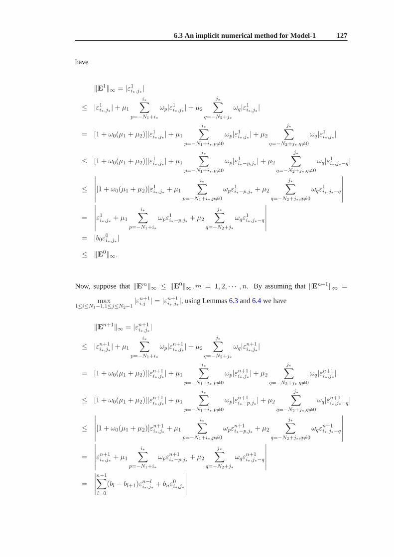
6.3 An implicit numerical method for Model-1 127
have
‖E1‖∞ = |ε1i∗,j∗ |
≤ |ε1i∗,j∗ |+ µ1
i∗∑
p=−N1+i∗
ωp|ε1i∗,j∗|+ µ2
j∗∑
q=−N2+j∗
ωq|ε1i∗,j∗|
= [1 + ω0(µ1 + µ2)]|ε1i∗ ,j∗|+ µ1
i∗∑
p=−N1+i∗,p 6=0
ωp|ε1i∗,j∗|+ µ2
j∗∑
q=−N2+j∗,q 6=0
ωq|ε1i∗,j∗|
≤ [1 + ω0(µ1 + µ2)]|ε1i∗ ,j∗|+ µ1
i∗∑
p=−N1+i∗,p 6=0
ωp|ε1i∗−p,j∗|+ µ2
j∗∑
q=−N2+j∗,q 6=0
ωq|ε1i∗,j∗−q|
≤
∣∣∣∣∣∣[1 + ω0(µ1 + µ2)]ε
1i∗,j∗ + µ1
i∗∑
p=−N1+i∗,p 6=0
ωpε1i∗−p,j∗ + µ2
j∗∑
q=−N2+j∗,q 6=0
ωqε1i∗,j∗−q
∣∣∣∣∣∣
=
∣∣∣∣∣∣ε1i∗,j∗ + µ1
i∗∑
p=−N1+i∗
ωpε1i∗−p,j∗ + µ2
j∗∑
q=−N2+j∗
ωqε1i∗,j∗−q
∣∣∣∣∣∣= |b0ε0i∗,j∗|
≤ ‖E0‖∞.
Now, suppose that‖Em‖∞ ≤ ‖E0‖∞,m = 1, 2, · · · , n. By assuming that‖En+1‖∞ =
max1≤i≤N1−1,1≤j≤N2−1
|εn+1i,j | = |εn+1
i∗,j∗|, using Lemmas6.3and6.4we have
‖En+1‖∞ = |εn+1i∗,j∗
|
≤ |εn+1i∗,j∗
|+ µ1
i∗∑
p=−N1+i∗
ωp|εn+1i∗,j∗
|+ µ2
j∗∑
q=−N2+j∗
ωq|εn+1i∗,j∗
|
= [1 + ω0(µ1 + µ2)]|εn+1i∗ ,j∗
|+ µ1
i∗∑
p=−N1+i∗,p 6=0
ωp|εn+1i∗,j∗
|+ µ2
j∗∑
q=−N2+j∗,q 6=0
ωq|εn+1i∗,j∗
|
≤ [1 + ω0(µ1 + µ2)]|εn+1i∗ ,j∗
|+ µ1
i∗∑
p=−N1+i∗,p 6=0
ωp|εn+1i∗−p,j∗
|+ µ2
j∗∑
q=−N2+j∗,q 6=0
ωq|εn+1i∗,j∗−q|
≤
∣∣∣∣∣∣[1 + ω0(µ1 + µ2)]ε
n+1i∗,j∗
+ µ1
i∗∑
p=−N1+i∗,p 6=0
ωpεn+1i∗−p,j∗
+ µ2
j∗∑
q=−N2+j∗,q 6=0
ωqεn+1i∗,j∗−q
∣∣∣∣∣∣
=
∣∣∣∣∣∣εn+1i∗,j∗
+ µ1
i∗∑
p=−N1+i∗
ωpεn+1i∗−p,j∗
+ µ2
j∗∑
q=−N2+j∗
ωqεn+1i∗,j∗−q
∣∣∣∣∣∣
=
∣∣∣∣∣
n−1∑
l=0
(bl − bl+1)εn−li∗,j∗
+ bnε0i∗,j∗
∣∣∣∣∣

6.3 An implicit numerical method for Model-1 128
≤n−1∑
l=0
(bl − bl+1)‖En−l‖∞ + bn‖E0‖∞
≤(
n−1∑
l=0
(bl − bl+1) + bn
)‖E0‖∞
= ‖E0‖∞.
Hence the implicit numerical method defined by (6.23) is unconditionally stable.
6.3.2 Convergence of the implicit numerical method
Settingeni,j = u(xi, yj, tn) − uni,j, and denotingRn = [en1,1, en2,1, · · · , enN1−1,N2−1]
T , then
R0 = 0. HereRn and0 are((N1 − 1)× (N2 − 1)) vectors, respectively.
From (6.15)-(6.23), the erroreni,j satisfies to the highest order expansion terms inτ , hx andhy
en+1i,j + µ1
i∑
p=−N1+i
ωpen+1i−p,j + µ2
j∑
q=−N2+j
ωqen+1i,j−q
=n−1∑
l=0
(bl − bl+1)en−li,j + C1τ
α(τ2−α + τ + h2x + h2y), (6.25)
for i = 1, 2, · · · , N1 − 1, j = 1, 2, · · · , N2 − 1.
Assuming‖Rn+1‖∞ = max1≤i≤N1−1,1≤j≤N2−1
|en+1i,j |, and using mathematical induction, we
have the following theorem.
Theorem 6.2. The implicit difference approximation defined by (6.23) is convergent, and there
is a positive constantC∗, such that
‖Rn+1‖∞ ≤ C∗(τ2−α + τ + h2x + h2y), n = 0, 1, 2, · · · , N. (6.26)
Proof. Whenn = 0, assume that‖R1‖∞ = max1≤i≤N1−1,1≤j≤N2−1
|e1i,j | = |e1i∗,j∗|. Similarly,
using inequality|Z1| − |Z2| ≤ |Z1 −Z2|, Lemmas6.3and6.4, and noting thatµ1, µ2 > 0, we

6.3 An implicit numerical method for Model-1 129
have
‖R1‖∞ = |e1i∗,j∗|
≤ |e1i∗,j∗|+ µ1
i∗∑
p=−N1+i∗
ωp|e1i∗,j∗|+ µ2
j∗∑
q=−N2+j∗
ωq|e1i∗,j∗|
= [1 + ω0(µ1 + µ2)]|e1i∗ ,j∗|+ µ1
i∗∑
p=−N1+i∗,p 6=0
ωp|e1i∗,j∗|+ µ2
j∗∑
q=−N2+j∗,q 6=0
ωq|e1i∗,j∗ |
≤ [1 + ω0(µ1 + µ2)]|e1i∗ ,j∗|+ µ1
i∗∑
p=−N1+i∗,p 6=0
ωp|e1i∗−p,j∗|+ µ2
j∗∑
q=−N2+j∗,q 6=0
ωq|e1i∗,j∗−q|
≤
∣∣∣∣∣∣e1i∗,j∗ + µ1
i∗∑
p=−N1+i∗
ωpe1i∗−p,j∗ + µ2
j∗∑
q=−N2+j∗
ωqe1i∗,j∗−q
∣∣∣∣∣∣.
Similar to the proof of the stability in Theorem6.1, this leads to
‖R1‖∞ ≤ C1τα(τ2−α + τ + h2x + h2y) = C1b
−10 τα(τ2−α + τ + h2x + h2y).
Now, suppose that‖Rm‖∞ ≤ C1b−1m−1τ
α(τ2−α+τ+h2x+h2y), m = 1, 2, · · · , n. By assuming
that‖Rn+1‖∞ = max1≤i≤N1−1,1≤j≤N2−1
|en+1i,j | = |en+1
i∗,j∗|, using Lemma6.3, and Lemma6.4and
(6.25) again, we have
‖Rn+1‖∞ = |en+1i∗,j∗
|
≤ |en+1i∗,j∗
|+ µ1
i∗∑
p=−N1+i∗
ωp|en+1i∗,j∗
|+ µ2
j∗∑
q=−N2+j∗
ωq|en+1i∗,j∗
|
= [1 + ω0(µ1 + µ2)]|en+1i∗ ,j∗
|+ µ1
i∗∑
p=−N1+i∗,p 6=0
ωp|en+1i∗,j∗
|+ µ2
j∗∑
q=−N2+j∗,q 6=0
ωq|en+1i∗,j∗
|
≤ [1 + ω0(µ1 + µ2)]|en+1i∗ ,j∗
|+ µ1
i∗∑
p=−N1+i∗,p 6=0
ωp|en+1i∗−p,j∗
|+ µ2
j∗∑
q=−N2+j∗,q 6=0
ωq|en+1i∗,j∗−q|
≤
∣∣∣∣∣∣en+1i∗,j∗
+ µ1
i∗∑
p=−N1+i∗
ωpen+1i∗−p,j∗
+ µ2
j∗∑
q=−N2+j∗
ωqen+1i∗,j∗−q
∣∣∣∣∣∣
=
∣∣∣∣∣
n−1∑
l=0
(bl − bl+1)en−li∗,j∗
+ C1τα(τ2−α + τ + h2x + h2y)
∣∣∣∣∣
≤n−1∑
l=0
(bl − bl+1)|en−li∗,j∗
|+ C1τα(τ2−α + τ + h2x + h2y)
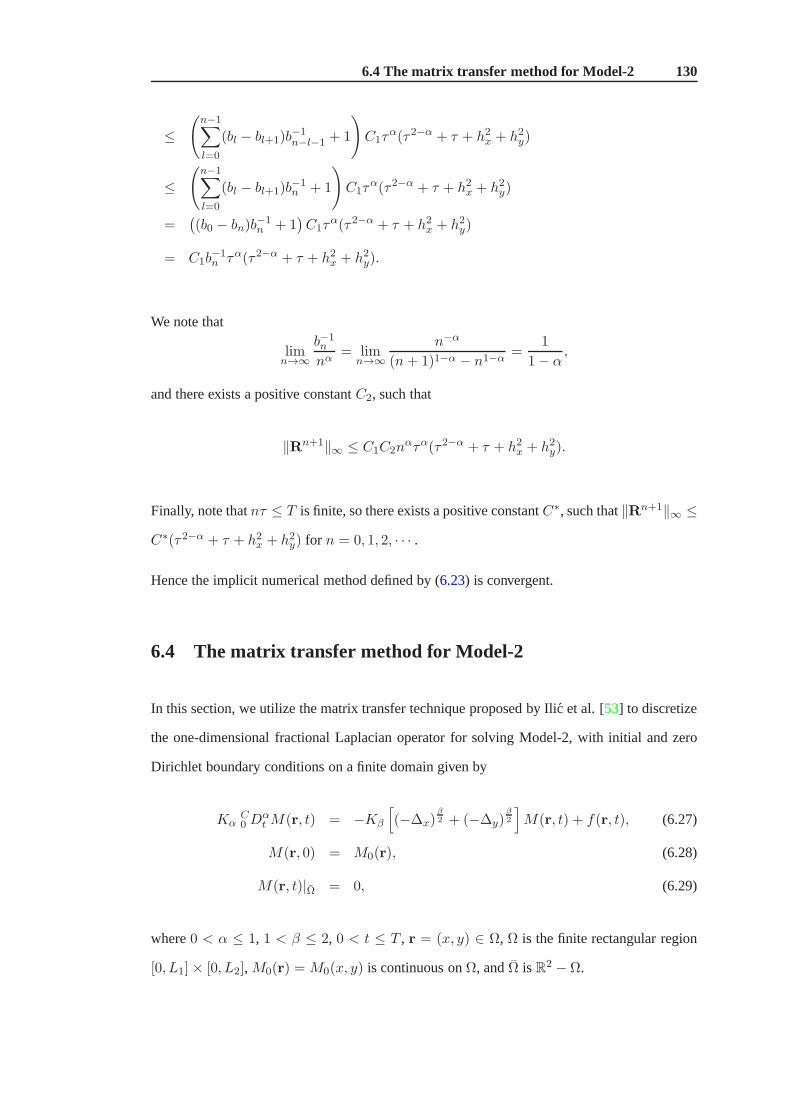
6.4 The matrix transfer method for Model-2 130
≤(
n−1∑
l=0
(bl − bl+1)b−1n−l−1 + 1
)C1τ
α(τ2−α + τ + h2x + h2y)
≤(
n−1∑
l=0
(bl − bl+1)b−1n + 1
)C1τ
α(τ2−α + τ + h2x + h2y)
=((b0 − bn)b
−1n + 1
)C1τ
α(τ2−α + τ + h2x + h2y)
= C1b−1n τα(τ2−α + τ + h2x + h2y).
We note that
limn→∞
b−1n
nα= lim
n→∞
n−α
(n+ 1)1−α − n1−α=
1
1− α,
and there exists a positive constantC2, such that
‖Rn+1‖∞ ≤ C1C2nατα(τ2−α + τ + h2x + h2y).
Finally, note thatnτ ≤ T is finite, so there exists a positive constantC∗, such that‖Rn+1‖∞ ≤
C∗(τ2−α + τ + h2x + h2y) for n = 0, 1, 2, · · · .
Hence the implicit numerical method defined by (6.23) is convergent.
6.4 The matrix transfer method for Model-2
In this section, we utilize the matrix transfer technique proposed by Ilic et al. [53] to discretize
the one-dimensional fractional Laplacian operator for solving Model-2, with initial and zero
Dirichlet boundary conditions on a finite domain given by
KαC0 D
αt M(r, t) = −Kβ
[(−∆x)
β2 + (−∆y)
β2
]M(r, t) + f(r, t), (6.27)
M(r, 0) = M0(r), (6.28)
M(r, t)|Ω = 0, (6.29)
where0 < α ≤ 1, 1 < β ≤ 2, 0 < t ≤ T , r = (x, y) ∈ Ω, Ω is the finite rectangular region
[0, L1]× [0, L2], M0(r) = M0(x, y) is continuous onΩ, andΩ isR2 −Ω.

6.4 The matrix transfer method for Model-2 131
Noting that the symbols(−∆x)β2 and(−∆y)
β2 have their usual meanings as a function of one-
dimensional Laplacian(−∆), which are defined in terms of their’s spectral decomposition. For
boundary value problems on finite domains, discrete eigenfunction expansions are used, where
Definition 6.2 is adopted.
The standard finite difference stencil with equal grid spacing in bothx andy directions, that is,
h = L1/N1 = L2/N2, will result in the tridiagonal approximate matrix representation of the
Laplacian operator(−∆x) and(−∆y), respectively, namely
A = m(−∆x) =1
h2diag(A∗, A∗, · · · , A∗), (6.30)
B = m(−∆y) =1
h2tridiag(−I, B∗,−I), (6.31)
wherem is the“coordinate” isomorphism,A∗ = tridiag(−1, 2,−1) andB∗ = 2I. Here
A,B ∈ R(N1−1)(N2−1)×(N1−1)(N2−1), A∗, B∗ ∈ R
(N1−1)×(N1−1), andI ∈ R(N1−1)×(N1−1) is
the identity matrix.
For a real nonsingular, symmetric matrixA, there exists a nonsingular matrixP x (P x ∈
R(N1−1)(N2−1)×(N1−1)(N2−1)), such that
A = P xΛxPxT
, (6.32)
whereΛx = diag(λx1 , λ
x2 , · · · , λx
(N1−1)(N2−1)) andλxk (k = 1, 2, · · · , (N1 − 1)(N2 − 1)) are
the eigenvalues ofA. Hence we obtain the matrix representation
m(−∆x)β2 = A
β2 = (P xΛxP
xT
)β2 = P xΛβ/2
x P xT
:= A∗∗ = (aij). (6.33)
Similarly, we have
m(−∆y)β2 = B
β2 = (P yΛyP
yT )β2 = P yΛβ/2
y P yT := B∗∗ = (b∗∗ij ), (6.34)
whereΛy = diag(λy1 , λ
y2, · · · , λ
y(N1−1)(N2−1)) andλy
k(k = 1, 2, · · · , (N1 − 1)(N2 − 1)) are
the eigenvalues ofB.
We denote the exact and numerical solutions ofM(r, t) asu(xi, yj , tn) anduni,j, respectively,
and the Caputo time fractional derivativeC0 D
αt is discretized as in equation (6.18), thus together

6.5 The matrix transfer method for Model-3 132
with equations (6.33) and (6.34), we can obtain the following numerical approximation of
Model-2 (6.27)-(6.29) as:
un+1i,j + µ
N2−1∑
p=1
N1−1∑
q=1
(a(i−1)(N1−1)+j,(p−1)(N1−1)+q + b∗∗(i−1)(N1−1)+j,(p−1)(N1−1)+q
)un+1pq
=
n−1∑
l=0
(bl − bl+1)un−li,j + bnu
0i,j + µ0f
ni,j, (6.35)
whereµ0 = ταΓ(2−α)Kα
, µ =Kβτ
αΓ(2−α)Kα
, i = 1, 2, · · · , N2 − 1, j = 1, 2, · · · , N1 − 1 and
n = 0, 1, 2, · · · , N − 1.
6.5 The matrix transfer method for Model-3
In this section, we utilize the matrix transfer technique proposed by Yang et al. [138] to
discretize the two-dimensional fractional Laplacian operator for solving Model-3, with initial
and zero Dirichlet boundary conditions on a finite domain given by
∂M(r, t)
∂t= −Kβ(−∆)
β2M(r, t) + f(r, t), (6.36)
M(r, 0) = M0(r), (6.37)
M(r, t)|Ω = 0, (6.38)
where∆ = ∂2
∂x2 + ∂2
∂y2 , 0 < α ≤ 1, 1 < β ≤ 2, 0 < t ≤ T , r = (x, y) ∈ Ω, Ω is the finite
rectangular region[0, L1]× [0, L2], M0(r) = M0(x, y) is continuous onΩ, andΩ isR2 − Ω.
The symbol(−∆)β2 has the usual meaning as a function of two-dimensional Laplacian(−∆),
which is defined in terms of its spectral decomposition. For boundary value problems on finite
domains, discrete eigenfunction expansions are used, where Definition6.3 is adopted.
The standard five-point finite difference stencil with equalgrid spacing in bothx and y
directions, that is,h = L1/N1 = L2/N2, will result in the block tridiagonal approximate
matrix representation of the Laplacian, namely
A♯ = m(−∆) =1
h2tridiag(−I, B♯,−I), (6.39)

6.6 Numerical results 133
where B♯ = tridiag(−1, 4,−1). Here A♯ ∈ R(N1−1)(N2−1)×(N1−1)(N2−1), B♯ ∈
R(N1−1)×(N1−1), andI ∈ R
(N1−1)×(N1−1) is the identity matrix.
Similarly, for a real nonsingular, symmetric matrixA♯, there exists a nonsingular matrixP
(P ∈ R(N1−1)(N2−1)×(N1−1)(N2−1)), such that
A♯ = PΛP T , (6.40)
whereΛ = diag(λ1, λ2, · · · , λ(N1−1)(N2−1)) andλk (k = 1, 2, · · · , (N1 − 1)(N2 − 1)) are
the eigenvalues ofA♯. Hence we obtain the matrix representation
m(−∆)β2 = A♯β
2 = (PΛP T )β2 = PΛβ/2P T := A♯♯ = (a♯♯ij). (6.41)
Let τ = T/N be the time step, and denote the numerical solutions ofM(r, t) asuni,j. Thus,
discretizing the time derivative using the backward differentiation formula and using equation
(6.41), we can obtain the following numerical approximation of Model-3 (6.36)-(6.38) as:
un+1i,j + τKβ
N2−1∑
p=1
N1−1∑
q=1
a♯♯(i−1)(N1−1)+j,(p−1)(N1−1)+qun+1pq = uni,j + τfn
i,j, (6.42)
wherei = 1, 2, · · · , N2 − 1, j = 1, 2, · · · , N1 − 1 andn = 0, 1, 2, · · · , N − 1.
6.6 Numerical results
In this section, we compare the numerical solutions of the three types of space and time
fractional Bloch-Torrey equations in 2D on a finite domain presented throughout Sections6.3-
6.5.
In Example6.1, we confirm the convergence order of the implicit numerical method for Model-
1 and show the solution behaviours of Models-1 and 2.

6.6 Numerical results 134
Example 6.1. Models-1 and 2 on a finite domain are considered, namely
Model − 1 : KαC0 D
αt M(r, t) = Kβ(
∂β
∂|x|β +∂β
∂|y|β )M(r, t) + f(r, t), (6.43)
Model − 2 : KαC0 D
αt M(r, t) = −Kβ
[(−∆x)
β2 + (−∆y)
β2
]M(r, t)
+f(r, t), (6.44)
with zero initial and zero Dirichlet boundary conditions
M(r, 0) = 0, (6.45)
M(r, t)|Ω = 0, (6.46)
where
f(r, t) =Kβt
α+β
2cos(βπ/2)
((2
Γ(3− β)[x2−β + (1− x)2−β ]− 12
Γ(4− β)[x3−β + (1− x)3−β]
+24
Γ(5− β)[x4−β + (1− x)4−β ]
)y2(1− y)2 +
(2
Γ(3− β)[y2−β + (1− y)2−β]
− 12
Γ(4− β)[y3−β + (1− y)3−β ] +
24
Γ(5− β)[y4−β + (1− y)4−β]
)x2(1− x)2
)
+KαΓ(α+ β + 1)
Γ(β + 1)tβx2(1− x)2y2(1− y)2,
and0 < α ≤ 1, 1 < β ≤ 2, 0 < t ≤ T , r = (x, y) ∈ Ω, Ω is the finite rectangular region
[0, 1] × [0, 1] andΩ isR2 − Ω.
The exact solution of this problem isM(r, t) = tα+βx2(1 − x)2y2(1 − y)2, which can be
verified by substituting directly into (6.43) or (6.44).
The relative error norm defined by
ǫ =
√√√√√
N1∑
i=0
N2∑
j=0
(uexactij − unumij )2
/
N1∑
i=0
N2∑
j=0
(uexactij )2
(6.47)
will be used to calculate the error between the exact and numerical solutions.
With Kα = Kβ = 1.0, α = 0.8, andβ = 1.8, Table6.1 lists the relative error between the
exact and numerical solutions obtained by the implicit numerical method for equation (6.43),
with spatial and temporal stepsτ1/2 = hx = hy = 1/4, 1/8, 1/16, 1/32 at timet = 1.

6.6 Numerical results 135
00.2
0.40.6
0.81
0
0.5
10
0.2
0.4
0.6
0.8
1
x 10−5
xy
M(x
,y,t
=10/
102)
(a)
00.2
0.40.6
0.81
0
0.5
10
0.2
0.4
0.6
0.8
1
x 10−5
xy
M(x
,y,t
=10/
102)
(b)
Figure 6.1: The comparison of solution profiles between Models-1 and 2 with spatial andtemporal stepsh = 1/16, τ = 1/102 at timet = 10/102 with Kα = Kβ = 1.0, tfinal = 1.0for α = 0.8 andβ = 1.8. (a) Implicit numerical method. (b) Matrix transfer technique.
From Table6.1, it can be seen that the
Error rate =error(h)2
error(12h)2≈ 4.
This is in good agreement with our theoretical analysis, namely the convergence order of the
implicit numerical method for equation (6.43) is (τ2−α + τ + h2x + h2y).
In addition, the comparison of solution profiles obtained bythe implicit numerical method
and the matrix transfer technique, respectively, with spatial and temporal stepsh = 1/16,
τ = 1/102 at timet = 10/102 with Kα = Kβ = 1.0, tfinal = 1.0 for α = 0.8 andβ = 1.8
is given in Figure6.1. From Figure6.1, it can be seen that the numerical solutions obtained
by the matrix transfer technique applied to Model-2 are in good agreement with those by the
implicit numerical method for Model-1.
Remark 6.1. A closer comparison of solution profiles between Models-1 and 2 on the unit
square with spatial and temporal stepsh = 1/16, τ = 1/102 at time t = 10/102 with
Kα = Kβ = 1.0, tfinal = 1.0 for y = 0.5, α = 0.8 andβ = 1.8 is given in Figure6.2. The
Table 6.1: Comparison of relative error for the implicit numerical method for Model-1 at timet = 1.0
τ1/2 = hx = hy Relative errorǫ Error rate
1/4 0.19893660 -1/8 0.04694709 4.241/16 0.01113693 4.221/32 0.00262580 4.24

6.6 Numerical results 136
0 0.2 0.4 0.6 0.8 10
0.5
1
1.5x 10
−5
distance x
M(x
,y,t
)
Exact solution
Model−1
Model−2
Figure 6.2: The comparison of solution profiles between Models-1 and 2 with spatial andtemporal stepsh = 1/16, τ = 1/102 at timet = 10/102 with Kα = Kβ = 1.0, tfinal = 1.0for y = 0.5, α = 0.8 andβ = 1.8, and the solutions are plotted along the centre line.
solutions are plotted along the centre line, and we can see that the solutions obtained from two
models both close to exact solution.
We now exhibit in Example6.2 a comparison of the numerical solutions between Models-1
and 2 with a nonlinear source term on a finite domain. We also investigate the equivalence of
the two models further, by studying the solution behaviour as the solution domain is extended.
Example 6.2. We now consider problems (6.43) and (6.44) with an initial source term and
zero Dirichlet boundary conditions on a finite domain given by
M(r, 0) = δ(x− 0.5, y − 0.5), (6.48)
M(r, t)|Ω = 0, (6.49)
where the nonlinear source termf(M, r, t) = 0.25M(r, t)[1 − M(r, t)] is Fisher’s growth
equation, and0 < α ≤ 1, 1 < β ≤ 2, 0 < t ≤ T , r = (x, y) ∈ Ω, Ω is the finite rectangular
region [0, 1] × [0, 1] andΩ isR2 −Ω.
The comparison of solution profiles obtained by the implicitnumerical method and matrix
transfer technique, respectively, with spatial and temporal stepsh = 1/16, τ = 1/102 at time
t = 10/102 with Kα = Kβ = 1.0, tfinal = 1.0 and forα = 0.8, β = 1.8 andα = 0.5, β =
1.5 are given in Figures6.3 and 6.4, respectively. We see that asα andβ are reduced the
profiles become more spiky, and that the numerical solutionsobtained by the matrix transfer
technique are in good agreement with those by the implicit numerical method.

6.6 Numerical results 137
00.2
0.40.6
0.81
0
0.5
10
2
4
6
8
x 10−3
xy
M(x
,y,t
=10/
102)
(a)
00.2
0.40.6
0.81
0
0.5
10
2
4
6
8
x 10−3
xy
M(x
,y,t
=10/
102)
(b)
Figure 6.3: The comparison of solution profiles between Models-1 and 2 with a nonlinearsource term with spatial and temporal stepsh = 1/16, τ = 1/102 at timet = 10/102 withKα = Kβ = 1.0, tfinal = 1.0 for α = 0.8 andβ = 1.8. (a) Implicit numerical method. (b)Matrix transfer technique.
00.2
0.40.6
0.81
0
0.5
10
0.005
0.01
0.015
xy
M(x
,y,t
=10/
102)
(a)
00.2
0.40.6
0.81
0
0.5
10
0.005
0.01
0.015
xy
M(x
,y,t
=10/
102)
(b)
Figure 6.4: The comparison of solution profiles between Models-1 and 2 with a nonlinearsource term with spatial and temporal stepsh = 1/16, τ = 1/102 at timet = 10/102 withKα = Kβ = 1.0, tfinal = 1.0 for α = 0.5 andβ = 1.5. (a) Implicit numerical method. (b)Matrix transfer technique.
In order to see the effect of domain size on the difference between the two models, we present
a comparison between the two with spatial and temporal stepsh = 1/8, τ = 1/64, Kα =
Kβ = 1.0, andα = 1.0 andβ = 1.8 for different t on the domain[−1, 1] × [−1, 1] (Figure
6.5) and domain[−2, 2] × [−2, 2] (Figure6.6). We see that as the domain size becomes larger
the solution for the two models closer in agreement.
In order to see the effect of time on the difference between the two models, we present a
comparison between the two with spatial and temporal stepsh = 1/8, τ = 1/64, Kα = Kβ =
1.0, andα = 1.0 andβ = 1.8 for different t on the domain[−2, 2] × [−2, 2] (Figure6.7) and
domain[−3, 3] × [−3, 3] (Figure6.8). We see that as the time becomes larger the differences

6.6 Numerical results 138
−1 −0.5 0 0.5 10
0.005
0.01
0.015
0.02
0.025
distance x
M(x
,y,t
)
Model−1
Model−2
(a)
−1 −0.5 0 0.5 10
1
2
3
4
5
6
7
8
9x 10
−3
distance x
M(x
,y,t
)
Model−1
Model−2
(b)
−1 −0.5 0 0.5 10
0.5
1
1.5
2
2.5x 10
−3
distance x
M(x
,y,t
)
Model−1
Model−2
(c)
−1 −0.5 0 0.5 10
0.5
1
1.5
2
2.5
3
3.5x 10
−4
distance x
M(x
,y,t
)
Model−1
Model−2
(d)
Figure 6.5: The comparison of solution profiles between Models-1 and 2 with a nonlinearsource term with zero Dirichlet boundary condition with spatial and temporal stepsh = 1/8,τ = 1/64 at a finite rectangular region[−1, 1] × [−1, 1] with Kα = Kβ = 1.0 for y = 0,α = 1.0 andβ = 1.8 for differentt.(a) t = 0.1. (b) t = 0.2. (c) t = 0.5. (d) t = 1.0.
in the solution profiles for the two models becomes larger, however, extending the domain can
reduce the difference between two models.
Figure6.9shows the error of solutions between the two models with spatial and temporal steps
h = 1/8, τ = 1/64, Kα = Kβ = 1.0, andα = 1.0 andβ = 1.8 for different t on the domain
[−2, 2] × [−2, 2] and domain[−3, 3] × [−3, 3]. We see that as the domain becomes larger the
error becomes smaller.
We repeat these simulations, except now we replace the zero Dirichlet boundary condition by
the homogeneous Neumann boundary condition
∂M(r, t)
∂r|Ω = 0. (6.50)
Figures6.10and6.11give the dynamics for the domains[−1, 1]×[−1, 1] and[−2, 2]×[−2, 2],
respectively. In this case, it can clearly be observed that the behaviour of the models,

6.6 Numerical results 139
−2 −1.5 −1 −0.5 0 0.5 1 1.5 20
0.005
0.01
0.015
0.02
0.025
distance x
M(x
,y,t
)
Model−1
Model−2
(a)
−2 −1.5 −1 −0.5 0 0.5 1 1.5 20
1
2
3
4
5
6
7
8
9x 10
−3
distance x
M(x
,y,t
)
Model−1
Model−2
(b)
−2 −1.5 −1 −0.5 0 0.5 1 1.5 20
0.5
1
1.5
2
2.5
3
3.5x 10
−3
distance x
M(x
,y,t
)
Model−1
Model−2
(c)
−2 −1.5 −1 −0.5 0 0.5 1 1.5 20
0.2
0.4
0.6
0.8
1
1.2
1.4
1.6x 10
−3
distance x
M(x
,y,t
)
Model−1
Model−2
(d)
Figure 6.6: The comparison of solution profiles between Models-1 and 2 with a nonlinearsource term with zero Dirichlet boundary condition with spatial and temporal stepsh = 1/8,τ = 1/64 at a finite rectangular region[−2, 2] × [−2, 2] with Kα = Kβ = 1.0 for y = 0,α = 1.0 andβ = 1.8 for differentt.(a) t = 0.1. (b) t = 0.2. (c) t = 0.5. (d) t = 1.0.
particularly at the boundaries at late times, is very different.
Finally, in Example6.3 we give a comparison of the numerical solutions between Models-1
and 3 with a nonlinear source term on a finite domain.
Example 6.3.
Model − 1 :∂M(r, t)
∂t= Kβ(
∂β
∂|x|β +∂β
∂|y|β )M(r, t) + f(M, r, t), (6.51)
Model − 3 :∂M(r, t)
∂t= −Kβ(−∆)
β2M(r, t) + f(M, r, t), (6.52)
with initial and zero Dirichlet boundary conditions on a finite domain
M(r, 0) = δ(x− 0.5, y − 0.5), (6.53)
M(r, t)|Ω = 0, (6.54)

6.6 Numerical results 140
−2 −1.5 −1 −0.5 0 0.5 1 1.5 20
0.005
0.01
0.015
0.02
0.025
distance x
M(x
,y,t
)
Model−1
Model−2
(a)
−2 −1.5 −1 −0.5 0 0.5 1 1.5 20
0.2
0.4
0.6
0.8
1
1.2
1.4
1.6x 10
−3
distance x
M(x
,y,t
)
Model−1
Model−2
(b)
−2 −1.5 −1 −0.5 0 0.5 1 1.5 20
1
2
3
4
5
6x 10
−4
distance x
M(x
,y,t
)
Model−1
Model−2
(c)
−2 −1.5 −1 −0.5 0 0.5 1 1.5 20
0.5
1
1.5
2
2.5
3
3.5
4x 10
−5
distance x
M(x
,y,t
)
Model−1
Model−2
(d)
−2 −1.5 −1 −0.5 0 0.5 1 1.5 20
0.5
1
1.5
2
2.5
3x 10
−6
distance x
M(x
,y,t
)
Model−1
Model−2
(e)
−2 −1.5 −1 −0.5 0 0.5 1 1.5 20
1
2
3
4
5
6x 10
−7
distance x
M(x
,y,t
)
Model−1
Model−2
(f )
Figure 6.7: The comparison of solution profiles between Models-1 and 2 with a nonlinearsource term with zero Dirichlet boundary condition with spatial and temporal stepsh = 1/8,τ = 1/64 at a finite rectangular region[−2, 2] × [−2, 2] with Kα = Kβ = 1.0 for y = 0,α = 1.0 andβ = 1.8 for different t.(a) t = 0.1. (b) t = 1. (c) t = 2. (d) t = 5. (e) t = 8. (f )t = 10.
where the nonlinear source termf(M, r, t) = 0.25M(r, t)[1 − M(r, t)] is Fisher’s growth
equation, and1 < β ≤ 2, 0 < t ≤ T , r = (x, y) ∈ Ω, Ω is the finite rectangular region
[0, 1] × [0, 1] andΩ isR2 − Ω.
The comparison of solution profiles of equations (6.51) and (6.52) obtained by the implicit
numerical method and matrix transfer technique, respectively, with spatial and temporal steps
h = 1/10, τ = 1/100 with Kβ = 1.0, tfinal = 1.0 for β = 1.8 at timet = 0.1 andt = 1.0,

6.6 Numerical results 141
−3 −2 −1 0 1 2 30
0.005
0.01
0.015
0.02
0.025
distance x
M(x
,y,t
)
Model−1
Model−2
(a)
−3 −2 −1 0 1 2 30
0.2
0.4
0.6
0.8
1
1.2
1.4
1.6
1.8x 10
−3
distance x
M(x
,y,t
)
Model−1
Model−2
(b)
−3 −2 −1 0 1 2 30
0.1
0.2
0.3
0.4
0.5
0.6
0.7
0.8
0.9
1x 10
−3
distance x
M(x
,y,t
)
Model−1
Model−2
(c)
−3 −2 −1 0 1 2 30
0.5
1
1.5
2
2.5
3
3.5x 10
−4
distance x
M(x
,y,t
)
Model−1
Model−2
(d)
−3 −2 −1 0 1 2 30
0.2
0.4
0.6
0.8
1
1.2
1.4x 10
−4
distance x
M(x
,y,t
)
Model−1
Model−2
(e)
−3 −2 −1 0 1 2 30
1
2
3
4
5
6
7x 10
−5
distance x
M(x
,y,t
)
Model−1
Model−2
(f )
Figure 6.8: The comparison of solution profiles between Models-1 and 2 with a nonlinearsource term with zero Dirichlet boundary condition with spatial and temporal stepsh = 1/8,τ = 1/64 at a finite rectangular region[−3, 3] × [−3, 3] with Kα = Kβ = 1.0 for y = 0,α = 1.0 andβ = 1.8 for different t.(a) t = 0.1. (b) t = 1. (c) t = 2. (d) t = 5. (e) t = 8. (f )t = 10.
respectively, are given in Figures6.12and6.13. From Figures6.12and6.13, it can be seen
clearly that the numerical solutions obtained from Model-3are not in good agreement with
those of the implicit numerical method from Model-1.

6.6 Numerical results 142
−2 −1.5 −1 −0.5 0 0.5 1 1.5 20
0.1
0.2
0.3
0.4
0.5
0.6
0.7
0.8
0.9
1x 10
−4
distance x
Err
or
t=0.1t=1t=2t=5t=8t=10
(a)
−3 −2 −1 0 1 2 30
0.1
0.2
0.3
0.4
0.5
0.6
0.7
0.8
0.9
1x 10
−4
distance x
Err
or
t=0.1t=1t=2t=5t=8t=10
(b)
Figure 6.9: The error of solutions between Models-1 and 2 with a nonlinear source term withzero Dirichlet boundary condition with spatial and temporal stepsh = 1/8, τ = 1/64 withKα = Kβ = 1.0 for y = 0, α = 1.0 andβ = 1.8 for different finite rectangular domains.(a)Finite rectangular region[−2, 2] × [−2, 2]. (b) Finite rectangular region[−3, 3] × [−3, 3].
−1 −0.5 0 0.5 10
0.005
0.01
0.015
0.02
0.025
distance x
M(x
,y,t
)
Model−1
Model−2
(a)
−1 −0.5 0 0.5 13
4
5
6
7
8
9
10x 10
−3
distance x
M(x
,y,t
)
Model−1
Model−2
(b)
−1 −0.5 0 0.5 13
3.5
4
4.5
5
5.5x 10
−3
distance x
M(x
,y,t
)
Model−1
Model−2
(c)
−1 −0.5 0 0.5 12
2.5
3
3.5
4
4.5
5
5.5
6x 10
−3
distance x
M(x
,y,t
)
Model−1
Model−2
(d)
Figure 6.10: The comparison of solution profiles between Models-1 and 2 with a nonlinearsource term with homogeneous Neumann boundary condition with spatial and temporal stepsh = 1/8, τ = 1/64 at a finite rectangular region[−1, 1] × [−1, 1] with Kα = Kβ = 1.0 fory = 0, α = 1.0 andβ = 1.8 for different t.(a) t = 0.1. (b) t = 0.2. (c) t = 0.5. (d) t = 1.0.

6.7 Conclusions 143
−2 −1.5 −1 −0.5 0 0.5 1 1.5 20
0.005
0.01
0.015
0.02
0.025
distance x
M(x
,y,t
)
Model−1
Model−2
(a)
−2 −1.5 −1 −0.5 0 0.5 1 1.5 20
1
2
3
4
5
6
7
8
9x 10
−3
distance x
M(x
,y,t
)
Model−1
Model−2
(b)
−2 −1.5 −1 −0.5 0 0.5 1 1.5 20.5
1
1.5
2
2.5
3
3.5x 10
−3
distance x
M(x
,y,t
)
Model−1
Model−2
(c)
−2 −1.5 −1 −0.5 0 0.5 1 1.5 20.8
1
1.2
1.4
1.6
1.8
2x 10
−3
distance x
M(x
,y,t
)
Model−1
Model−2
(d)
Figure 6.11: The comparison of solution profiles between Models-1 and 2 with a nonlinearsource term with homogeneous Neumann boundary condition with spatial and temporal stepsh = 1/8, τ = 1/64 at a finite rectangular region[−2, 2] × [−2, 2] with Kα = Kβ = 1.0 fory = 0, α = 1.0 andβ = 1.8 for different t.(a) t = 0.1. (b) t = 0.2. (c) t = 0.5. (d) t = 1.0.
00.2
0.40.6
0.81
0
0.5
10
0.002
0.004
0.006
0.008
0.01
xy
M(x
,y,t
=0.1
)
(a)
00.2
0.40.6
0.81
0
0.5
10
0.002
0.004
0.006
0.008
0.01
xy
M(x
,y,t
=0.1
)
(b)
Figure 6.12: The comparison of solution profiles between Models-1 and 3 with a nonlinearsource term with spatial and temporal stepsh = 1/10, τ = 1/100 at time t = 0.1 withKβ = 1.0, tfinal = 1.0 for β = 1.8. (a) Implicit numerical method. (b) Matrix transfertechnique.
6.7 Conclusions
In this chapter, we compare the numerical solutions obtained from an implicit numerical
method and the matrix transfer technique, for three types ofspace and time fractional Bloch-
Torrey equations in two dimensions based on a Riesz derivative and two forms of a fractional

6.7 Conclusions 144
00.2
0.40.6
0.81
0
0.5
10
0.2
0.4
0.6
0.8
1
x 10−6
xy
M(x
,y,t
=1)
(a)
00.2
0.40.6
0.81
0
0.5
10
2
4
6
8
x 10−8
xy
M(x
,y,t
=1)
(b)
Figure 6.13: The comparison of solution profiles between Models-1 and 3 with a nonlinearsource term with spatial and temporal stepsh = 1/10, τ = 1/100 at time t = 1.0 withKβ = 1.0, tfinal = 1.0 for β = 1.8. (a) Implicit numerical method. (b) Matrix transfertechnique.
Laplacian in one dimension and two dimensions, respectively. The main focus is on finite
domains with zero Dirichlet boundary conditions. We show that these formulations are not
equivalent, but that as the size of the domain increases, Model 1 and Model 2 are increasingly
similar. However, this is not the case for homogeneous Neumann boundary conditions
where Model 1 and Model 2 are very different. Furthermore, the one dimensional and two
dimensional forms for the Laplacian can also be different even in the case of zero Dirichlet
boundary conditions. This shows that the dynamics of fractional models very much depend on
the boundary condition in the case of finite domains, and thateven in the case of zero Dirichlet
boundary conditions we must take considerable care in deciding which model we should use
and in interpreting the simulation results. In the future weplan to compare our methods
for solving the space and time fractional models studied here with the methods proposed
by Podlubny et al. [112]. However in that paper all examples are in one spatial dimension,
although it is claimed that the approach is easily extendable to higher dimensions.

CHAPTER 7
The use of a Riesz fractional differential-based
approach for texture enhancement in image processing
7.1 Introduction
Texture enhancement is one of the most important issues to bedealt with in image processing,
and plays a substantial role in medical imaging [44]. The quality of images, especially the
texture, is more and more significant for supporting clinical diagnosis of pathology.
The current image enhancement algorithms are typically based on integer order differential
mask operators that include the Sobel, Roberts, Prewit and Laplacian techniques [44, 106, 113].
After the comparison of images enhanced using first and second order derivatives, it has been
concluded that the integer order differential operator hasseveral shortcomings. In particular,
processing using first order masks produces wide edges, while second order masks are sensitive
to noise and generate double responses when the grey-scale changes [106, 151].
Recently, the value of fractional calculus has been widely demonstrated for various applications
in science and engineering [24, 23, 21, 22, 73, 76, 77, 78, 79, 80, 90, 117, 135, 137, 138, 139,

7.1 Introduction 146
140, 141, 146, 149, 150, 155, 157, 158]. These successes have motivated researchers to apply
fractional derivatives to digital image processing [42, 43, 86, 108, 114, 115, 122, 151]. Zhang
et al. [151] developed an algorithm based on the Riemann-Liouville definition and applied the
resulting model with a fractional derivative index betweenone and two to enhance the texture
and edges of a digital image. Sejdic et al. [122] investigated the use of the fractional Fourier
transform in signal processing. Pesquet-Popescu and Vehel [108] developed stochastic fractal
models for image processing. Mathieu et al. [86] applied fractional differentiation for edge
detection. Gao et al. [42] applied a quaternion fractional differential based on theGrunwald-
Letnikov definition to a color image. Gao et al. [43] applied an improved fractional differential
operator based on a piecewise quaternion for image enhancement. Pu et al. [115] proposed
various algorithms based on the Grunwald-Letnikov definition, which do well in grey images,
but they result in the color image being distorted in the RGB (red, green and blue) space.
In contrast with the standard derivative, the fractional derivative of a direct current or low-
frequency signal is usually nonzero [42, 114, 115, 151]. Thus, the fractional differential
not only nonlinearly preserves the contour features of the smooth area, but maintains a
high-frequency edge feature in those areas where the grey changes considerably. It also
preserves a high-frequency texture detail feature in thoseareas where the grey does not change
significantly.
In this chapter we build upon the classical and first order fractional mask approaches to
overcome defects in enhancement and color image distortion, by investigating the performance
of two fractional differential algorithms based on the Riesz [140] fractional differential
operator.
The structure of the remainder of this chapter is follows. Insection 7.2, we give the
theoretical analysis for implementing fractional differential masks, and deduce two fractional
derivative algorithms, FCD-1 and FCD-2, based on the Riesz fractional differential operator.
Finally, we illustrate that our algorithms provide higher precision and better visual effects for
texture enhancement than Pu’s algorithm (YiFeiPU-1) [115] when applied to medical imaging
applications.

7.2 The improved fractional differential mask 147
7.2 The improved fractional differential mask
We first recall thev-order(0 < v ≤ 2) Riesz fractional derivative∂vu(t)∂|t|v given in [140] for the
infinite interval−∞ < t < +∞:
∂vu(t)
∂|t|v = −cv
(∂v
∂tv+
∂v
∂(−t)v
)u(t), (7.1)
wherecv = 12 cos(πv
2) (v 6= 1), n− 1 < v ≤ n,
∂vu(t)
∂tv=
1
Γ(n− v)
∂n
∂tn
∫ t
−∞
u(ξ)dξ
(t− ξ)v+1−n, (7.2)
∂vu(t)
∂(−t)v=
(−1)n
Γ(n− v)
∂n
∂tn
∫ +∞
t
u(ξ)dξ
(ξ − t)v+1−n. (7.3)
The Riesz fractional derivative can be approximated using the following second order fractional
centered difference scheme given in [104] with steph:
∂vu(x)
∂|x|v = −h−v∞∑
k=−∞
ω∗ku(x− kh) +O(h2), (7.4)
where the coefficients are defined by
ω∗k =
(−1)kΓ(v + 1)
Γ(v2 − k + 1)Γ(v2 + k + 1), p = 0,∓1,∓2, · · · . (7.5)
Lemma 7.1. The coefficientsω∗k (k ∈ N) satisfy:
1. ω∗0 ≥ 0, ω∗
−k = ω∗k ≤ 0 for all |k| ≥ 1;
2.∞∑
k=−∞
ω∗k = 0;
3. For any positive integern,m with n < m, we haven∑
k=−m+n
ω∗k > 0.
Proof. See [20, 104].
We deduce the following two fractional differential algorithms, FCD-1 and FCD-2, based on
the Riesz fractional differential operator (7.1).
Firstly, when0 < v < 1, usingΓ(y)Γ(1−y) = πsin(πy) (0 < y < 1), we haveΓ(v2 )Γ(1− v
2 ) =

7.2 The improved fractional differential mask 148
πsin(πv
2) andΓ(v)Γ(1 − v) = π
sin(πv) =π
2 sin(πv2) cos(πv
2) , then we have
1
2 cos(πv2 )=
Γ(v)Γ(1− v)
Γ(v2 )Γ(1− v2 )
, 0 < v < 1. (7.6)
Using (7.6), equation (7.4) can be rewritten as
∂vu(t)
∂|t|v = − 1
2 cos(πv2 )
(∂v
∂tv+
∂v
∂(−t)v
)u(t)
≈ − 1
2 cos(πv2 )hv
[∞∑
k=0
ωku(t− kh) +
0∑
k=−∞
ωku(t− kh)
], (7.7)
where
ω0 = − Γ(1− v2)
vΓ(1+ v2)Γ(−v) ,
ωk =(−1)k+1Γ( v
2)Γ(1− v
2)
Γ( v2−k+1)Γ( v
2+k+1)Γ(−v) , k = ±1,±2, · · · .
(7.8)
Returning to our problem of texture enhancement for image processing, it is well known that
an object processed by a computer or digital filter is the limit number [114, 115, 151] and the
biggest variable of the grey-level of an image signal is alsolimited, in the sense that the shortest
distance for a change in the grey-level image must be at an adjacent pixel. Thus, pixels are used
to measure the duration of a two-dimensional digital images(x, y) with respect to two variables
x andy. Here, the duration is the dimension of the image matrix assuming that the duration of
x andy is [0,X] and [0, Y ], respectively. The uniform distances for thex andy-coordinates
arehx = XN = 1 andhy = Y
N = 1 and the number of divisions areNx = [X/hx] = [X] and
Ny = [Y/hy] = [Y ].
As an example for a two dimensional digital images(x, y) at pixel (x∗, y∗) on the positive
x-axis with the region[0, x∗], theN + 1 pixels aresN (x∗, y∗) = s(0, y∗), sN−1(x∗, y∗) =
s(h, y∗), · · · , sk(x∗, y∗) = s(x∗ − kh, y∗), · · · , s0(x∗, y∗) = s(x∗, y∗). After truncation, the
anteriorn + 1 approximate fractional centered difference of the fractional partial differential
respectively on the positivex-axis is expressed as:
∂vs(x, y)
∂xv∼= − 1
2 cos(πv2 )hv
n∑
k=0
ωks(x− kh, y), 0 < v < 1. (7.9)
In order to obtain the fractional derivative for the eight symmetric directions and ensure that the
fractional differential masks have an anti-rotation capability, Pu et al. [115] implemented eight

7.2 The improved fractional differential mask 149
fractional differential masks that are positioned respectively on the negativex-axis, positive
x-axis, negativey-axis, positivey-axis, left downward diagonal, right upward diagonal, left
upward diagonal, and right downward diagonal. They are correspondingly denoted byWl(l =
1, 2, . . . , 8) (see Figure7.1). This terminology is noted as the YiFeiPU-1 operator.
In Figure7.1, Cs0 is the mask coefficient associated with the pixel of interest. Whenn = 2m,
one can implement a(2m + 1) × (2m + 1) fractional differential mask. To ensure that the
fractional differential mask has a certain center, in general, n is taken as an even number.
It is known that digital image processing is based on direct processing for discrete pixels, and
the algorithm also takes into consideration an airspace filtering scheme [115]. The principle
of the airspace filter is to move the mask pixel by pixel. As faras the properties of the grey
image and color image are concerned, there are considerabledifferences. Thus, there are two
algorithms for the fractional differential mask, one for the grey image and the other for the color
image. To treat theNx × Ny digital grey images(x, y), Pu et al. [115] present a convolution
filter on the above eight directions by using the YiFeiPU-1 operator in the(2m+1)×(2m+1)
masks, and propose that the eight fractional differential masks are computed using
sl(x, y) =
Nl∑
i=Ml
Ql∑
j=Pl
Wl(i, j)s(x + i, y + j), l = 1, 2, 3, 4, (7.10)
sl(x, y) =
Nl∑
i=Ml
Ql∑
j=Pl
√2−v
Wl(i, j)s(x + i, y + j), l = 5, 6, 7, 8. (7.11)
wherel = 1 (negativex-axis),M1 = −2m,N1 = 0, P1 = −m,Q1 = m; l = 2 (positive
x-axis),M2 = 0, N2 = 2m,P2 = −m,Q2 = m; l = 3 (negativey-axis),M3 = −m,N3 =
m,P3 = −2m,Q3 = 0; l = 4 (positivey-axis),M4 = −m,N4 = m,P4 = 0, Q4 = 2m;
l = 5 (left downward diagonal),M5 = 0, N5 = 2m,P5 = −2m,Q5 = 0; l = 6 (right
upward diagonal),M6 = −2m,N6 = 0, P6 = 0, Q6 = 2m; l = 7 (left upward diagonal),
M7 = −2m,N7 = 0, P7 = −2m,Q7 = 0; and l = 8 (right downward diagonal),M8 =
0, N8 = 2m,P8 = 0, Q8 = 2m.
Thus, we have
s(x, y) =
8∑l=1
sl(x, y)
4n∑
k=0
(1 +√2−v
)Csk
, (7.12)

7.2 The improved fractional differential mask 150
(a)W1 (negativex-axis); (e)W5 (left downward diagonal);
(b)W2 (positivex-axis); (f)W6 (right upward diagonal);
(c) W3 (negativey-axis); (g)W7 (left upward diagonal);
(d) W4 (positivey-axis); (h)W8 (right downward diagonal).
Figure 7.1: Fractional differential mask for the eight directions given by Pu et al. [115].

7.2 The improved fractional differential mask 151
whereCsk is the mask coefficient (see equations (7.13) and (7.15)).
As for the digital color image, the algorithm is similar to that for a grey image, but the R, G,
B components use the fractional differential respectively. Since there are correlations among
the RGB elements, the grey-level value is usually limited tothe range[0, 255], the elements of
RGB will be nonlinearly enhanced when the orderv is big. The correlation of element R, G and
B may be destroyed, which leads to color distortion. Therefore, we often apply the fractional
differential to the digital color image in a color space of YCrCb and HSV (hue, saturation and
value), also called HSB (where B is for brightness).
We implement the fractional mask respectively on the eight symmetric directions using what
we call the FCD-1 operator, having the same structure but with different coefficients than
YiFeiPU-1. The mask coefficients of the FCD-1 operator are given by
Cs0 = − 12 cos(πv
2)hvω0
Csk = − 12 cos(πv
2)hvωk (k = 1, 2, · · · , n)
, 0 < v < 1, (7.13)
which ensures that the fractional differential operator FCD-1 produces a sparse matrix having
dimensionn+1. Moreover, all the coefficients depend on the fractional differential orderv. It
also can be proved that the sum of the coefficients is nonzero,which is a remarkable difference
between the fractional differential mask and the integer version.
Similarly, when1 < v < 2, usingΓ(y)Γ(1 − y) = πsin(πy) (0 < y < 1), we haveΓ(v2 )Γ(1 −
v2 ) =
πsin(πv
2) andΓ(v − 1)Γ(2− v) = π
sin[π(v−1)] =π
− sin(πv) =π
−2 sin(πv2) cos(πv
2) , and
1
2 cos(πv2 )= −Γ(v − 1)Γ(2 − v)
Γ(v2 )Γ(1− v2)
, 1 < v < 2. (7.14)
we can obtain the fractional mask FCD-2 with the coefficients
Cs0 = 12 cos(πv
2)hv
(v−1)Γ(1− v2)
Γ(1+ v2)Γ(2−v)
Csk = 12 cos(πv
2)hv
(−1)kv(v−1)Γ( v2)Γ(1− v
2)
Γ( v2−k+1)Γ( v
2+k+1)Γ(2−v) (k = 1, 2, · · · , n)
, 1 < v < 2. (7.15)

7.3 Experiments and analysis 152
7.3 Experiments and analysis
In this section, we apply our algorithms to image enhancement of grey and color images.
We also compare our methods with YiFeiPU-1 to show that they have better performance in
terms of precision and give an improved visual effect for texture enhancement. We adopt the
fractional derivative with index0 < v < 1 to enhance the texture details, and use the index
1 < v < 2 to enhance the edge and texture details for digital image processing. For the
simulations performed here, all the algorithms are writtenand executed using MATLAB. For
example, Algorithm7.1shows the algorithm for a grey image.
Input : Read original grey image, and add Gaussian noise with mean 0and variance
0.01.
Output : s(x, y)
Choosem = 2, n = 4 and mask5× 5;
Compute the mask coefficientsCskusing either equation (7.13) (0 < v < 1) or (7.15)
(1 < v < 2);
Compute the dimensionNx ×Ny of the image matrix;
for x = 2 : Nx − 1 do
for y = 2 : Ny − 1 do
for l = 1 : 8 do
Computesl(x, y) using equations (7.10) and (7.11);
end
Computes(x, y) using equation (7.12);
end
end
Display adjusted images(x, y).Algorithm 7.1: Algorithm for grey image
In Figure 7.2, we compare our method FCD-1 with YiFeiPU-1 and the traditional integer
differential methods involving the Sobel operator and Laplacian operator on the Lena image
[106] with Gaussian noise having mean0 and variance0.01. We can see from Figure7.2 that
integer differential methods cannot be used for texture enhancement, because they enhance
high-frequency marginal information where the grey-levelchanges greatly, but cannot preserve
the low-frequency contour information in smooth areas. They also cannot enhance the texture

7.3 Experiments and analysis 153
Table 7.1: SNR with Gaussian noise having mean0 and variance0.01 with v = 0.5 and mask5× 5 for YiFeiPU-1 and FCD-1
Operators for comparison SNRSobel 3.4854Laplacian 3.2889YiFeiPU-1 8.3112FCD-1 10.1877
Table 7.2: SNR with Gaussian noise having mean0 and variance0.01 between FCD-1 andYiFeiPU-1 withv = 0.5
The dimensions of mask YiFeiPU-1 FCD-13× 3 10.7370 13.27095× 5 8.3112 10.18777× 7 7.3078 8.82639× 9 6.7438 8.037111 × 11 6.3833 7.529713 × 13 6.1325 7.1614
details in those areas where grey-levels have little change. We also can see from the figures that
the image resulting from our method FCD-1 has the best definition and the best visual effect.
We note in particular that the visual effect offered by FCD-1is better than that of YiFeiPU-1
when using the same fractional order and same mask dimensions.
We define the rate of the signal to noise
SNR = (Asignal/Anoise)2, (7.16)
where A is root mean square amplitude. Table7.1exhibits the rate of the signal to noise results
(SNR) for the traditional integer differential methods using Sobel and Laplacian operators for
the Lena image, and we choosev = 0.5 and mask5 × 5 for YiFeiPU-1 and FCD-1. It can
be seen clearly from Table7.1 that FCD-1 has a higher value than the YiFeiPU-1, Sobel and
Laplacian operators, which implies a more superior textureenhancement.
For the indexv = 0.5, we show in Table7.2a comparison of SNR for the Lena image generated
using FCD-1 and YiFeiPU-1. It can be seen clearly from Table7.2 that again, with the same
dimensions of the mask, FCD-1 has the higher SNR value.
Table7.3 shows the SNR ofFCD − 1 with v = 0.5 with Gaussian noise having mean0 and
different variance.

7.3 Experiments and analysis 154
(a) (d)
(b) (e)
(c) (f)
Figure 7.2: The contrast effects of Gaussian noise image enhancement with mean0 andvariance0.01 and its fractional differential using YiFeiPU-1 and FCD-1.(a) Original Lenaimage, (b) grey-scale noise image, (c) Sobel operator, (d) Laplacian operator, (e)0.5-orderYiFeiPU-1 with mask3× 3, (f) 0.5-order FCD-1 with mask3× 3.

7.3 Experiments and analysis 155
Table 7.3: SNR ofFCD − 1 with v = 0.5 with Gaussian noise having mean0 and differentvariance
Mask\Variance 0.01 0.001 0.0001 0.000013× 3 13.2709 16.0782 15.3897 15.24505× 5 10.1877 14.8973 15.6114 15.66117× 7 8.8263 13.1775 15.1130 15.37659× 9 8.0371 11.9314 13.7864 14.048811× 11 7.5297 11.0611 12.8527 13.1053
Table 7.4: The rate of the noise power ofFCD − 1 with v = 0.5 with Gaussian noise havingmean0 and different variance
Mask\Variance 0.01 0.001 0.0001 0.000013× 3 0.011208 0.006270 0.007836 0.0082325× 5 0.025014 0.007392 0.006815 0.0067237× 7 0.036986 0.010741 0.006627 0.0062879× 9 0.046667 0.014874 0.009245 0.00866111× 11 0.061384 0.022331 0.014223 0.013342
Table7.4shows the noise power ofFCD − 1 with v = 0.5 with Gaussian noise having mean
0 and different variance.
Table7.5shows the SNR ofFCD−1 with Gaussian noise having mean0 and variance0.0001
with variousv for the dimensions of mask= 3× 3, 5× 5 and7× 7, respectively.
We now present two experiments to test our methods on a human brain image from a patient
diagnosed with Parkinson’s disease before surgery from St Andrew’s War Memorial Hospital,
Brisbane, Australia.
By respectively applying the fractional differential to the three elements of H, S and I in HSI
color space, and then reverting to RGB color space, one can gain a color image without
Table 7.5: SNR ofFCD − 1 with Gaussian noise having mean0 and variance0.0001 withvariousv for the dimensions of mask= 3× 3, 5× 5 and7× 7 respectively
v 3× 3 5× 5 7× 7 9× 9 11× 11
0.1 16.3283 16.2691 16.2051 16.2264 16.23930.2 16.1586 15.8918 15.8526 16.1796 16.48400.3 15.8808 15.6681 16.0560 16.4346 16.55410.4 15.4833 15.7491 16.0014 15.8416 15.08200.5 15.3897 15.6114 15.1130 13.7846 12.85110.6 15.2847 14.9782 13.1537 11.8709 10.99150.7 15.1371 13.4535 11.4359 10.2145 9.37810.8 14.8136 11.8482 9.8909 8.7508 7.96740.9 14.1886 10.3870 8.5179 7.4461 6.7435

7.3 Experiments and analysis 156
(a) (b)
(c) (d)
Figure 7.3: Comparison of texture details between originalfractional anisotropy weightedorientation map and its fractional differential using FCD-1 with mask= 5 × 5. (a) Originalimage, (b)0.3-order FCD-1, (c)0.5-order FCD-1, (d)0.7-order FCD-1.
distortion. Figure7.3 shows the comparison of the texture details between an original
fractional anisotropy weighted orientation map and its fractional differential using FCD-1 with
mask= 5 × 5. From Figure7.3, it can be seen that, the backgrounds of the original image
are those areas with smooth textures, which comprise the most comprehensive texture details;
moreover its grey-level values have little variation. The foreground of the original image is
those areas with high-frequency verge, and its grey-level values have more variability.
In addition, Figure7.4shows the comparison of texture-segmentation performancebetween an
original grey image and its fractional differential version using FCD-2 with mask= 5×5. It can
be qualitatively established from Figure7.4 that the fractional differential in1 < v < 2 is able

7.4 Conclusions 157
to segment texture as defined by image contrast. As the order increases, the tissue sharpening
effect is more pronounced.
7.4 Conclusions
The application of fractional differentials to the analysis and processing of image signals, in
particular those associated with digital images, has attracted considerable recent attention.
In this chapter, we derive two fractional differential algorithms FCD-1 and FCD-2 based on the
Riesz fractional differential operator for grey and color image enhancement. The experiments
show that our algorithms are able to produce better results than traditional integer differential
based algorithms and fractional methods based on the Grunwald-Letnikov definition. This
is the case where nonlinear enhancement of high-frequency edges and texture information
does not change significantly. We conjecture that the use of asymmetric second order Riesz
fractional operator, instead of a one-sided first order fractional Grunwald-Letnikov operator,
can provide better texture enhancement of the image, which is confirmed in our results.
Furthermore, we have performed a simple sensitivity study to obtain a reasonable tradeoff
between precision and visual effect. In this chapter we onlyreport the range of values
considered. In future work we will perform rigorous evaluation of how the fractional order
affects the performance of our algorithm.

7.4 Conclusions 158
(a) (d)
(b) (e)
(c) (f)
Figure 7.4: Comparison of texture-segmentation performance between original grey imageand its fractional differential using FCD-2 with mask= 5×5. (a) Original image, (b)1.2-orderFCD-2, (c)1.4-order FCD-2, (d)1.5-order FCD-2, (e)1.6-order FCD-2, (f)1.8-order FCD-2.

CHAPTER 8
Conclusions
Recently, some fractional models [14, 82, 83, 84, 85, 109, 154] have been proposed for
the Bloch equations to describe numerous experimental situations including heterogeneous,
porous or composite materials and study anomalous diffusion in the human brain. However,
effective numerical methods and supporting error analysesfor the fractional Bloch equation
and fractional Bloch-Torrey equation are still under development.
Recall that the main objectives of this thesis are to developnew efficient numerical methods
and supporting convergence and stability analysis for solving the time, space and space and
time fractional dynamical systems involving fractional derivatives, and new efficient fractional
differential-based approach for texture enhancement in image processing. Six published papers
present the solutions of the time fractional diffusion equation [145], space fractional diffusion
equation [145], time fractional Bloch equation [142], anomalous fractional Bloch equation
[142] and space and time fractional Bloch-Torrey equation [140, 141, 143], respectively,
together with a new efficient fractional differential-based approach for texture enhancement
in image processing [144]. These papers, which are presented in Chapters2 to 7 of the thesis
and form the backbone of the theory associated with the newlydeveloped numerical methods.

8.1 Summary and Discussion 160
In the next section, we discuss the contributions of this thesis in greater detail. The chapter
concludes with some recommendations for future research.
8.1 Summary and Discussion
In Chapter2 we considered the computational simulation of brain connectivity using diffusion
tensor magnetic resonance imaging (DT-MRI). DT-MRI is a technique used to measure the
diffusion properties of water molecules in biological tissues [9]. The anisotropy of the diffusion
tensor is of particular interest in brain images, as it is related to white matter fibre tracts.
Depending on the interrelation of the eigenvalues, diffusion can be divided into the three
different cases [69] of linear diffusion, planar diffusion and spherical diffusion.
We derived numerical methods to analyse brain images, and developed one dimensional
fractional models to study the anomalous diffusion behaviour in the white matter of the brain.
In addition, brain image data was compared for a patient withParkinson’s disease before and
after surgery. The simulated information can provide the surgeon with a more fundamental
understanding of the impact of surgery on the diffusion behavior in the white matter of the
brain.
In Chapter3 we considered the fractional Bloch equations involving thetime fractional Bloch
equations (TFBE) and the anomalous fractional Bloch equations (AFBE). Magin et al. [83] and
Velasco et al. [130] have demonstrated that a fractional calculus based diffusion model can be
successfully applied to analysing diffusion images of human brain tissues and this new model
provided new insights into further investigations of tissue structures and the microenvironment.
We derived an analytical solution and an effective predictor-corrector method (PCM) for
solving the TFBE. The error analysis for PCM was establishedtheoretically, under the
assumption that the source term satisfies a Lipschitz condition. In addition, we proposed
an effective implicit numerical method (INM) for solving the AFBE. The stability and
convergence of the INM were analysed systematically. This was the first time that such
numerical schemes were presented for the fractional Bloch equations.
We presented some numerical examples to demonstrate the effectiveness of PCM and INM.
The numerical results show that the spin dynamics are generally fractional order, although they

8.1 Summary and Discussion 161
become the classical case when the fractional order of differentiation is set at1. We concluded
that fractional models can effectively simulate the spin dynamics in a static magnetic field, and
can play an important role for us understanding NMR for complex systems.
In Chapter4 we considered the space and time fractional Bloch-Torrey equation (ST-FBTE), an
equation that has attracted considerable recent attention[82, 154], to examine the connection
between fractional order dynamics and diffusion. This was the first time that a numerical
scheme was presented for the ST-FBTE.
We derived an analytical solution using a spectral representation method for solving the ST-
FBTE in fractional Laplacian form. In addition, we proposedan implicit numerical method for
solving the ST-FBTE in Riesz form. The Caputo time fractional derivative is treated using a
finite difference method. We discretized the Riesz space fractional derivative using the shifted
Grunwald-Letnikov method. The stability and convergenceof the implicit numerical method
are analysed systematically.
Due to the complexity of the analytic solution given in this chapter, and the computational
overheads necessary to perform the simulations for nuclearmagnetic resonance in three
dimensions, we presented a preliminary study based on a two-dimensional example to confirm
our theoretical analysis. We used our numerical method to simulate a problem of practical
importance involving a nonlinear source term. Our results highlighted the impact of the
fractional indices on the shape of the solution profile. Overall, the diffusion coefficient has a
significant effect, especially for fractional values ofα. The most significant effects in terms of
the spikiness of the profile occurs as both fractional orderα andβ are simultaneously reduced.
In Chapter5 we did further investigation of the ST-FBTE in three-dimensions. Since fractional
derivatives are nonlocal and have history dependence, fractional problems generally require a
large amount of CPU time if traditional implicit schemes based on Gaussian elimination are
used. Alternating direction implicit (ADI) schemes reducethe multidimensional problem into
a series of independent one-dimensional problems and are thus computationally efficient. In
order to overcome the computational difficulty mentioned above for Chapter4, we proposed
a computationally effective fractional alternating direction method (FADM) for solving the
ST-FBTE in three-dimensions. After discretizing the Caputo time fractional derivative and

8.1 Summary and Discussion 162
Riesz space fractional derivative by a finite difference method and the shifted Grunwald-
Letnikov method, respectively, we adopted the ADI method toconstruct a computationally
effective FADM for solving the ST-FBTE in three-dimensional. We proved that the FADM is
unconditionally stable and convergent, which had not been done previously.
We used our numerical method to simulate a problem of practical importance involving a
nonlinear source term. In all cases we concluded that the FADM is more computationally
efficient than the standard implicit techniques solved using either direct or indirect methods,
because the computational expense associated with the solution of the large dense matrix that
is generated as a result of the three-dimensional discretisation is avoided. This was the first
time that the three-dimensional numerical results obtained for the ST-FBTE.
In Chapter6 we performed a numerical investigation of three types of ST-FBTE in two
dimensions: Model-1 with the Riesz fractional derivative;Model-2 with the one-dimensional
fractional Laplacian operator; and Model-3 with the two-dimensional fractional Laplacian
operator.
We proposed a spatially second-order accurate implicit numerical method for Model-1 whereby
we discretized the Riesz fractional derivative using a fractional centered difference. The
stability and convergence of the implicit numerical methodare analysed systematically. We
utilized the matrix transfer technique for solving Model-2and Model-3. Some numerical
results were given to show the behaviours of these three models especially on varying domain
sizes with zero Dirichlet boundary conditions. We showed that these formulations are not
equivalent, but that as the size of the domain increases, Model-1 and Model-2 are increasingly
similar. However, this is not the case for homogeneous Neumann boundary conditions
where Model-1 and Model-2 are very different. Furthermore,the one dimensional and two
dimensional forms for the Laplacian can also be different even in the case of zero Dirichlet
boundary conditions. This shows that the dynamics of fractional models very much depend on
the boundary condition in the case of finite domains, and thateven in the case of zero Dirichlet
boundary conditions we must take considerable care in deciding which model we should use
for interpreting the simulation results. We feel this is an important contribution to the literature.
In Chapter7 we considered the use of a Riesz fractional differential-based approach for texture
enhancement in image processing. The application of fractional differentials to the analysis and

8.2 Directions for Future Research 163
processing of image signals, in particular those associated with digital images, has attracted
considerable recent attentions.
We derived two fractional differential algorithms FCD-1 and FCD-2 based on the Riesz
fractional differential operator for grey and color image enhancement. The experiments showed
that our algorithms are able to produce better results than traditional integer differential based
algorithms and fractional methods based on the Grunwald-Letnikov definition. This is the
case where nonlinear enhancement of high-frequency edges and texture information does not
change significantly. We conjectured that the use of a symmetric second order Riesz fractional
operator, instead of a one- sided first order fractional Grunwald-Letnikov operator, can provide
better texture enhancement of the image, which is confirmed in our results. Furthermore, we
had performed a simple sensitivity study to obtain a reasonable tradeoff between precision and
visual effect. In this chapter we only report the range of values considered. In future work
we will perform rigorous evaluation of how the fractional order affects the performance of our
algorithm.
8.2 Directions for Future Research
There are a number of extensions and applications to the methods presented in this thesis that
could be pursued in the future. In particular, the followingareas would be recommended for
further investigation.
• Mathematical methods for anomalous diffusion images
In Chapter2 we considered the computational simulation of brain connectivity using
diffusion tensor magnetic resonance imaging (DT-MRI). We used fractional anisotropy
(FA) to measure the diffusion anisotropy. Hall and Barrick [50] pointed out that the
model of restricted diffusion commonly employed in the analysis of diffusion MR data
is not valid in complex environments, such as human brain tissue. They described an
imaging method based on the theory of anomalous diffusion and showed that images
based on environmental complexity may be constructed from diffusion-weighted MR
images, where the anomalous exponentγ < 1 and fractal dimensiondw were measured
from diffusion-weighted MRI data. They defined a new measureof anisotropy using

8.2 Directions for Future Research 164
Anomalous Anisotropy (AA), which is a generalization of FA,and given by
AA =
√N
N − 1
∑Ni=1(γi− < γ >)2∑N
i=1 γ2i
,
where N is the number of directions,γi is the anomalous exponent in the directioni and
< γ > is the mean (i.e. directionally averaged) exponent.
In addition to this, it would be benificial to explore how to obtain a reasonable tradeoff
between precision and visual effect. It would be strongly recommended to perform a
rigorous evaluation of the fractional orderv given in Chapter7, which is also an open and
interesting problem. One idea would be to dynamically adjust the fractional differential
order according to the image local statistics and structural features.
• New effective numerical methods for solving the ST-FBTE
Aside from the finite difference method, the finite element methods [39, 40, 41, 117, 138]
for solving fractional partial differential equations have been proposed. Fix and Roop
[41] proved existence and uniqueness of the least squares finiteelement solution of
a fractional order two-point boundary value problem. They proved the optimal error
estimates for piecewise linear trial elements. Roop [117] investigated the computational
aspects of the Galerkin approximation using continuous piecewise polynomial basis
functions on a regular triangulation of the bounded domain in R2. Ervin and Roop
[39] presented a theoretical framework for the Galerkin finite element approximation to
the steady state fractional advection dispersion equation(FADE). Appropriate fractional
derivative spaces were defined and shown to be equivalent to the usual fractional
dimension Sobolev spacesHs. They proved the existence and uniqueness results of
the variational solution, and derived error estimates for the Galerkin finite element
approximation to the FADE. Ervin and Roop [40] discussed the steady state fractional
advection dispersion equation (FADE-RD) on bounded domains in Rd. Appropriate
fractional derivative spaces were defined and shown to be equivalent to the fractional
dimensional Sobolev spaces. They presented a theoretical framework for the variational
solution, proved the existence and uniqueness results of the variation solution, and
obtained the error estimates for the finite element approximation to the FADE-RD. Yang
et al. [138] used the finite difference and finite element methods to solve the time-space

8.2 Directions for Future Research 165
fractional diffusion equation in two dimensions. They investigated both the Lanczos
and M-Lanczos methods for approximating the matrix function vector product, and
proposed the error bounds to terminate the Lanczos subspaceexpansion. Because the
finite element method can be used to simulate practical problem even when complex
transition zone are involved, it would be interesting to consider the use of the finite
element method for solving the ST-FBTE.
• Investigate three types of ST-FBTE in Chapter6 with non-homogeneous Dirichlet or
Neumann conditions in 2D or homogeneous Dirichlet or Neumann conditions in 3D
In Chapter6, we performed a numerical investigation of three types of ST-FBTE
in two dimensions: Model-1 with the Riesz fractional derivative; Model-2 with the
one-dimensional fractional Laplacian operator; and Model-3 with the two-dimensional
fractional Laplacian operator. Some numerical results were given to show the behaviours
of these three models especially on varying domain sizes with zero Dirichlet boundary
conditions. We showed that these formulations are not equivalent, but that as the size of
the domain increases, Model-1 and Model-2 are increasinglysimilar. However, this is not
the case for homogeneous Neumann boundary conditions whereModel-1 and Model-2
are very different. Furthermore, the one-dimensional and two-dimensional forms for the
Laplacian can also be different even in the case of zero Dirichlet boundary conditions.
In order to better decide which model we should use for interpreting the simulation
results, it would be interesting to consider these three models in two dimensions with
non-homogeneous Dirichlet or Neumann conditions. It wouldalso be interesting and
challenging to generalise results to higher dimensional problems, e.g. 3-D problems.

Bibliography
[1] A. Abragam.Principles of nuclear magnetism. Oxford University Press, Oxford, 2002.
[2] O. P. Agrawal. Solution for a fractional diffusion-waveequation defined in a bounded
domain.Nonlinear Dynamics, 29: 145-155, 2002.
[3] K. Al-Khaled and S. Momani. An approximate solution for afractional diffusion-
wave equation using the decomposition method.Applied Mathematics and Computation,
165(2): 473-483, 2005.
[4] V. V. Anh, N. N. Leonenko. Spectral analysis of fractional kinetic equations with random
data.J.Stat.Phys., 104: 1349-1387, 2001.
[5] B. Baeumer, M. Kovacs and M. M. Meerschaert. Numerical solutions for fractional
reaction diffusion equations.Computers and Mathematics with Applications, 55: 2212-
2226, 2008.
[6] A. V. Barzykin. Exact solution of the Torrey-Bloch equation for a spin echo in restricted
geometries.Phys. Rev. B, 58(21): 14171C14174, 1998.
[7] P. Basser, J. Mattiello, D. Le Bihan. Estimation of the effective self-diffusion tensor from
the NMR spin echo.Journal Of Magnetic Resonance Series B, 103: 247-254, 1994.

BIBLIOGRAPHY 167
[8] P. J. Basser, C. Pierpaoli. A simplified method to measurethe diffusion tensor from seven
MR images.Magnetic Resonance in Medicine, 39: 928-934, 1998.
[9] P. G. Batchelor, D. L. G. Hill, F. Calamante and D. Atkinson. Study of connectivity in the
brain using the full diffusion tensor from MRI.Proceedings of Information Processing in
Medical Imaging IPMI, 2082: 121-133, 2001.
[10] W. Benger, H. Bartsch, H. Hege, H. Kitzler. Visualizingneuronal structures in the human
brain via diffusion tensor MRI.Intern. J. Neuroscience, 116: 461-514, 2006.
[11] D. A. Benson, S. W. Wheatcraft and M. M. Meerschaert. Application of a fractional
advection-dispersion equation.Water Resources Research, 36(6): 1403-1412, 2000.
[12] K. Bennett, K. Schmainda, R. Bennett, D. Rowe, H. Lu and J. Hyde. Characterization of
continuously distributed cortical water diffusion rates with a stretched exponential model.
Magnetic Resonance in Medicine, 50(4): 727-734, 2003.
[13] G. Berenschot. Visualization of diffusion tensor imaging. Master’s Thesis, 2003.
[14] S. Bhalekar, V. Daftardar-Gejji, D. Baleanu and R. Magin. Fractional Bloch equation with
delay.Computers and Mathematics with Applications, 61(5): 1355-1365, 2011.
[15] S. Bhalekar, V. Daftardar-Gejji, D. Baleanu and R. Magin. Transient chaos in fractional
Bloch equations.Computers and Mathematics with Applications, 64(10): 3367-3376,
2012.
[16] B. Bonilla, M. Rivero, J. J. Trujillo. On systems of linear fractional differential equations
with constant coefficients.Applied Mathematics and Computation, 187: 68-78, 2007.
[17] W. G. Bradley. History of medical imaging.Proceedings of the American Philosophical
Society, 152(3): 349-361, 2008.
[18] A. Bueno-Orovio, D. Kay and K. Burrage. Fourier spectral methods for fractional-in-
space reaction-diffusion equations.Journal of Computational Physics, in press, 2013.
[19] K. Burrage, N. Hale and D. Kay. An Efficient Implicit FEM scheme for fractional-in-
space reaction-diffusion equations.SIAM Journal on Scientific Computing, 34(4): A2145-
A2172, 2012.
BIBLIOGRAPHY 168
[20] C. Celik and M. Duman. Crank-Nicolson method for the fractional diffusion equation
with the Riesz fractional derivative.Journal of Computational Physics, 231: 1743-1750,
2012.
[21] C. Chen, F. Liu and V. Anh. Numerical analysis of the Rayleigh-Stokes problem for a
heated generalized second grade fluid with fractional derivatives.Appl. Math. Comp.,
204: 340-351, 2008.
[22] C. Chen, F. Liu and V. Anh. A Fourier method and an extrapolation technique for Stokes’
first problem for a heated generalized second grade fluid withfractional derivative.J.
Comp. Appl. Math., 223: 777-789, 2009.
[23] C Chen, F. Liu and K. Burrage. Finite difference methodsand a Fourier analysis for the
fractional reaction-subdiffusion equation.Appl. Math. Comp., 198: 754-769, 2008.
[24] C. Chen, F. Liu, I. Turner, V. Anh. A Fourier method for the fractional diffusion equation
describing sub-diffusion.J. Comput. Phys., 227: 886-897, 2007.
[25] C. Chen, F. Liu, I. Turner, V. Anh. Numerical schemes andmultivariate extrapolation of
a two-dimensional anomalous sub-diffusion equation.Numer. Algor., 54: 1-21, 2010.
[26] S. Chen, F. Liu. ADI-Euler and extrapolation methods for the two-dimensional fractional
advection-dispersion equation.Journal of Applied Mathematics and Computing, 26: 295-
311, 2008.
[27] S. Chen, F. Liu, I. Turner and V. Anh. An implicit numerical method for the two-
dimensional fractional percolation equation.Appl. Comp. Math., 219(9): 4322-4331,
2013.
[28] J. Chen, F. Liu and V. Anh. Analytical solution for the time-fractional telegraph
equation by the method of separating variables.Journal of Mathematical Analysis and
Applications, 338(2): 1364-1377, 2007.
[29] C. Clark and D. Le Bihan. Water diffusion compartmentation and anisotropy at high b
values in the human brain.Magnetic Resonance in Medicine, 44(6): 852-859, 2000.
[30] K. Diethelm.The Analysis of Fractional Differential Equations: An Application Oriented
Exposition Using Differential Operators of Caputo Type. Springer, Berlin, 2010.

BIBLIOGRAPHY 169
[31] K. Diethelm, N. J. Ford and A. D. Freed. Detailed error analysis for a fractional Adams
method.Numerical Algorithms, 36: 31-52, 2004.
[32] K. Diethelm and A. D. Freed. The FracPECE subroutine forthe numerical solution of
differential equations of fractional order, in:Forschung und wissenschaftliches Rechnen:
Beitrage zum Heinz-Billing-Preis 1998, eds. S. Heinzel and T. Plesser (Gesellschaft fur
wissenschaftliche Datenverarbeitung, Gottingen), 57-71, 1999.
[33] I. S. Donskaya, A. R. kessel. Bloch equations with diffusion terms for rotational motion
in fluids.Soviet Physics Journal, 16(1): 29-32, 1973.
[34] J. Jr. Douglas. Alternating direction method for threespace variables.Numerische
Mathematik, 4(1): 41-63, 1961.
[35] J. Jr. Douglas and J. Gunn. A general formulation of alternating direction methods. Part
I. Parabolic and hyperbolic problems.Numerische Mathematik, 6(1): 428-453, 1964.
[36] A. Elliott. Medical imaging.Nuclear Instruments and Methods in Physics Research A,
546: 1-13, 2005.
[37] A. Erdelyi (ed.).Higher Transcendental Functions. vol. 3, McGrawHill, New York, 1955.
[38] A. Erdelyi, W. Magnus, F. Oberhettinger and F. Tricomi. Higher transcendental functions.
vol. I-III, Krieger Pub., Melbourne, Florida, 1981.
[39] V. J. Ervin and J. P. Roop. Variational solution of the fractional advection dispersion
equation.Numer. Meth. PDE, 22(3): 558-576, 2006.
[40] V. J. Ervin and J. P. Roop. Variational solution of fractional advection dispersion equations
on bounded domains inRd. Numer. Meth. PDE, 23(2): 256-281, 2007.
[41] G. J. Fix and J. P. Roop. Least squares finite-element solution of a fractional order two-
point boundary value problem.Computers and Mathematics with Applications, 48(7-8):
1017-1033, 2004.
[42] C. B. Gao, J. L. Zhou, J. R. Hu, F. N. Lang. Edge detection of colour image based on
quaternion fractional diffeerential.IET Image Processing, 5(3): 261-272, 2011.

BIBLIOGRAPHY 170
[43] C. B. Gao, J. L. Zhou, X. Q. Zheng, F. N. Lang. Image enhancement based on improved
fractional differentiation.Journal of Computational Information Systems, 7(1): 257-264,
2011.
[44] R. C. Gonzalez, R. E. Woods.Digital Image Processing. Third Edition. Prentice Hall,
New Jersey, USA, 2007.
[45] R. Gorenflo and E. A. Abdel-Rehim. Convergence of the Gr¨unwald-Letnikov scheme for
time-fractional diffusion.Journal of Computational and Applied Mathematics, 205(2):
871-881, 2007.
[46] R. Gorenflo and F. Mainardi. Random walk models for space-fractional diffusion
processes.Fractional Calculus and Applied Analysis, 1(2): 167-191, 1998.
[47] R. Gorenflo, F. Mainardi, D. Moretti, G. Pagnini and P. Paradisi. Discrete random walk
models for space-time fractional diffusion.Chemical Physics, 284: 521-544, 2002.
[48] R. Gorenflo, F. Mainardi, D. Moretti and P. Paradisi. Time fractional diffusion: A discrete
random walk approach.Nonlinear Dynamics, 29: 129-143, 2002.
[49] E. Hairer, G. Wanner.Solving ordinary differential equations II: stiff and differential-
algebraic problems. Springer, Berlin, 1991.
[50] M. Hall and T. Barrick. From diffusion-weighted MRI to anomalous diffusion imaging.
Magnetic Resonance in Medicine, 59(3): 447-455, 2008.
[51] R. Hilfer. Applications of fractional calculus in physics. World Scientific Publishing,
New York, 2000.
[52] M. Ilic, F. Liu, I. Turner and V. Anh. Numerical approximation of a fractional-in-space
diffusion equation, I.Fractional Calculus and Applied Analysis, 8(3): 323-341, 2005.
[53] M. Ilic, F. Liu, I. Turner and V. Anh. Numerical approximation of a fractional-in-space
diffusion equation (II)-with nonhomogeneous boundary conditions.Fractional Calculus
and Applied Analysis, 9(4): 333-349, 2006.
[54] M. Ilic, I. W. Turner and D. P. Simpson. A restarted Lanczos approximation to functions
of a symmetric matrix.IMA Journal of Numerical Analysis, 30(4): 1044-1061, 2010.

BIBLIOGRAPHY 171
[55] H. Jafari and V. Daftardar-Gejji. Solving linear and nonlinear fractional diffusion and
wave equations by Adomian decomposition.Applied Mathematics and Computation,
180(2): 488-497, 2006.
[56] T. H. Jochimsena, A. Schaferb, R. Bammera and M. E. Moseleya. Efficient
simulation of magnetic resonance imaging with Bloch-Torrey equations using intra-voxel
magnetization gradients.Journal of Magnetic Resonance, 180(1): 29C38, 2006.
[57] J. I. Kaplan. Application of the Diffusion-Modified Bloch Equation to Electron Spin
Resonance in Ordinary and Ferromagnetic Metals.Physical Review, 115(3): 575-577,
1959.
[58] J. Karger, H. Pfeifer, G. Vojta. Time correlation during anomalous diffusion in fractal
systems and signal attenuation in NMR field-gradient spectroscopy.Phys. Rev. A, 37:
4514-4517, 1988.
[59] J. Karger, G. Vojta. On the use of NMR pulsed field-gradient spectroscopy for the study
of anomalous diffusion in fractal networks.Chem. Phys. Lett., 141: 411-413, 1987.
[60] V. M. Kenkre, E. Fukushima and D. Sheltraw. Simple solutions of the Torrey-Bloch
equations in the NMR study of molecular diffusion.Journal of Magnetic Resonance,
128(1): 62-69, 1997.
[61] C. Khalil, C. Hancart, V. Le Thuc, C. Chantelot, D. Chechin, A. Cotten. Diffusion tensor
imaging and tractography of the median nerve in carpal tunnel syndrome: preliminary
results.Eur Radiol, 18: 2283-2291, 2008.
[62] K. Khanafer, K. Vafai and A. Kangarlu. Water diffusion in biomedical systems as related
to magnetic resonance imaging.Magnetic Resonance Imaging, 21(1): 17-31, 2003.
[63] A. A. Kilbas, H. M. Srivastava and J. J. Trujillo.Theory and Applications of fractional
differential equations. Elsevier, Amsterdam, 2006.
[64] T. A. M. Langlands and B. I. Henry. The accuracy and stability of an implicit solution
method for the fractional diffusion equation.Journal of Computational Physics, 205(2):
719-736, 2005.

BIBLIOGRAPHY 172
[65] D. Le Bihan. Molecular diffusion, tissue microdynamics and microstructure.NMR in
Biomedicine, 8(7): 375-386, 1995.
[66] D. Le Bihan. The ’wet mind’: water and functional neuroimaging.Physics in Medicine
and Biology, 52(7): R57-R90, 2007.
[67] D. Le Bihan, E. Breton, D. Lallemand, P. Grenier, E. Cabanis, M. Laval-Jeantet. MR
imaging of intravoxel incoherent motions: application to diffusion and perfusion in
neurologic disorders.Radiology, 161: 401-407, 1986.
[68] D. Le Bihan, J. Mangin, C. Poupon, C. A. Clark, S. Pappata, N.Molko and H.Chabriat.
Diffusion tensor imaging: concepts and applications.Journal of Magnetic Resonance
Imaging, 13: 534-546, 2001.
[69] A. Leemans. Modeling and processing of diffusion tensor magnetic resonance images for
improved analysis of brain connectivity.PhD thesis, University of Antwerp, Belgium,
2006.
[70] M. Ledoux. The Geometry of Markov Diffusion Generators. Annales de la Faculte des
Sciences de Toulouse, 6(9): 305-366, 2000.
[71] C. Li, Y. Wu, R. Ye.Recent Advances in Applied Nonlinear Dynamics with Numerical
Analysis: Fractional Dynamics, Network Dynamics, Classical Dynamics and Fractal
Dynamics with Their Numerical Simulations. World Scientific, Singapore, 2013.
[72] C. P. Li, F. H. Zeng. Finite difference methods for fractional differential
equations. Int. J. Bifurcation Chaos, 22(4): 1230014 (28 pages), 2012. DOI:
10.1142/S0218127412300145.
[73] F. Liu, V. Anh, I. Turner. Numerical solution of the space fractional Fokker-Planck
equation.Journal of Computational and Applied Mathematics, 166: 209-219, 2004.
[74] F. Liu, V. Anh, I. Turner and P. Zhuang. Time fractional advection-dispersion equation.
Journal of Applied Mathematics and Computing, 13(1-2): 233-246, 2003.
[75] F. Liu and K. Burrage. Novel techniques in parameter estimation for fractional dynamical
models arising from biological systems.Computer and Mathematics with Application,
62(3): 822-833, 2011.

BIBLIOGRAPHY 173
[76] F. Liu, S. Shen, V. Anh, I. Turner. Analysis of a discretenon-Markovian random walk
approximation for the time fractional diffusion equation.ANZIAM J., 46(E): 488-504,
2005.
[77] F. Liu, Q. Yang and I. Turner. Two new implicit numericalmethods for the fractional
cable equation.Journal of Computational and Nonlinear Dynamics, 6(1): 011009. 2011.
[78] F. Liu, P. Zhuang, V. Anh, I. Turner and K. Burrage. Stability and convergence of the
difference methods for the space-time fractional advection-diffusion equation.Applied
Mathematics and Computation, 91: 12-20, 2007.
[79] Q. Liu, F. Liu, I. Turner and V. Anh. Numerical simulation for the 3D seepage flow with
fractional derivatives in porous media.IMA Journal of Applied Mathematics, 74: 201-
229, 2009.
[80] Q. Liu, Y. Gu, P. Zhuang, F. Liu and Y. Nie. An implicit RBFmeshless approach for time
fractional diffusion equations.Computational Mechanics, 48(1): 1-12, 2011.
[81] Y. Luchko and R. Gorenflo. An operational method for solving fractional differential
equations with the Caputo derivatives.Acta Mathematica Vietnamica, 24(2): 207-233,
1999.
[82] R. Magin, O. Abdullah, D. Baleanu and X. Zhou. Anomalousdiffusion expressed through
fractional order differential operators in the Bloch-Torrey equation.Journal of Magnetic
Resonance, 190(2): 255-270, 2008.
[83] R. Magin, X. Feng, D. Baleanu. Solving the fractional order Bloch equation.Concepts in
Magnetic Resonance PartA, 34A(1): 16-23, 2009.
[84] R. Magin, X. Feng, D. Baleanu. Fractional calculus in NMR. Magn. Reson. Engr., 34:
16-23, 2009.
[85] R. Magin, W. Li, M. Velasco, J. Trujillo, D. Reiter, A. Morgenstern and R. Spencer.
Anomalous NMR relaxation in cartilage matrix components and native cartilage:
Fractional-order models.Journal of Magnetic Resonance, 210(2): 184-191, 2011.
[86] B. Mathieu, P. Melchior, A. Oustaloup, Ch. Ceyral. Fractional differentiation for edge
detection.Signal Processing, 83(11): 2421-2432, 2003.

BIBLIOGRAPHY 174
[87] R. M. Mazo. Brownian motion: fluctuations, dynamics, and applications. Oxford
University Press, Oxford, 2002.
[88] M. M. Meerschaert, H. Scheffler and C. Tadjeran. Finite difference methods for two-
dimensional fractional dispersion equation.Journal of Computational Physics, 211: 249-
261, 2006.
[89] M. M. Meerschaert and A. Sikorskii.Stochastic Models for Fractional Calculus. De
Gruyter, Berlin, 2012.
[90] M. M. Meerschaert and C. Tadjeran. Finite difference approximations for fractional
advection-dispersion flow equations.Journal of Computational and Applied
Mathematics, 172: 65-77, 2004.
[91] E. R. Melhem, S. Mori, G. Mukundan, M. A. Kraut, M. G. Pomper and P. C. M. van
Zijl. Diffusion tensor MR imaging of the brain and white matter tractography.American
Journal of Roentgenology, 178: 3-16, 2002.
[92] K. D. Merboldt, W. Hanicke and J. Frahm. Self-diffusionNMR imaging using stimulated
echoes.Journal of Magnetic Resonance, 64: 479-486, 1985.
[93] R. Metzler and J. Klafter. The random walks guide to anomalous diffusion: A fractional
dynamics approach.Phys. Rep., 339: 1-77, 2000.
[94] R. K. Miller, A. N. Michel. Ordinary differential equations. Academic Press, New York,
1982.
[95] S. Momani and Z. Odibat. Numerical solutions of the space-time fractional advection-
dispersion equation.Numerical Methods for Partial Differential Equations, 24(6): 1416-
1429, 2008.
[96] S. Mori. Introduction to Diffusion Tensor Imaging. Elsevier B.V., 2007.
[97] S. Momani and P. C. M. van Zijl. Fiber tracking: principles and strategies-a technical
review.NMR in Biomedicine, 15(7-8): 468-480, 2002.
[98] M. E. Moseley, Y. Cohen, J. Mintorovitch, L. Chileuitt,H. Shimizu, J. Kucharczyk, M. F.
Wendland and P. R. Weinstein. Early detection of regional cerebral ischemia in cats:

BIBLIOGRAPHY 175
Comparison of diffusion- andT2-weighted MRI and spectroscopy.Magnetic Resonance
in Medicine, 14(2): 330-346, 1990.
[99] P. Mukherjee, J. I. Berman, S. W. Chung, C. P. Hess and C. P. Henry. Diffusion tensor
MR imaging and fiber tractography: theoretic underpinnings. Phy. Review, AJNR Am J
Neuroradiol, 29: 632-642, 2008.
[100] R. Mulkern, H. Gudbjartsson, C. Westin, H. Zengingonul, W. gartner, C. Guttman, R.
Robertson, W. Kyriakos, R. Schwartz, D. Holzman, F. Jolesz and D. Le Bihan. Multi-
component apparent diffusion coefficients in human brain.NMR in Biomedicine, 12(1):
51-62, 1999.
[101] D. G. Nishimura.Principles of Magnetic Resonance Imaging. Stanford University,
California, 1996.
[102] D. Norris. The effects of microscopic tissue parameters on the diffusion weighted
magnetic resonance imaging experiment.NMR in Biomedicine, 14(2): 77-93, 2001.
[103] L. ODonnell, S. Haker and C. Westin. New approaches to estimation of white matter
connectivity in diffusion tensor MRI: elliptic PDEs and geodesics in tensor-warped space.
Medical Image Computing and Computer-Assisted Intervention ł MICCAI 2002 Lecture
Notes in Computer Science, 2488: 459-466, 2002.
[104] M. D. Ortigueira. Riesz potential operators and inverses via fractional centred
derivatives.International Journal of Mathematics and Mathematical Sciences, Article
ID 48391: 1-12, 2006.
[105] E. Ozarslan, P. Basser, T. Shepherd, P. Thelwall, B. Vemuri andS. Blackband.
Observation of anomalous diffusion in excised tissue by characterizing the diffusion time
dependence of the MR signal.Journal of Magnetic Resonance, 183(2): 315-323, 2006.
[106] C. S. Panda, S. Patnaik. Filtering corrupted image andedge detection in restored
grayscale image using derivative filters.International Journal of Image Processing, 3(3):
105-119, 2009.
[107] D. W. Peaceman and H. H. Rachford. The numerical solution of parabolic and elliptic
differential equations.J. Soc. Indust. Appl. Math., 3: 28-41, 1955.

BIBLIOGRAPHY 176
[108] B. Pesquet-Popescu and J. L. Vehel. Stochastic fractal models for image processing.
IEEE Signal Processing Magazine, 19(5): 48-62, 2002.
[109] I. Petras. Modeling and numerical analysis of fractional-order Bloch equations.
Computers and Mathematics with Applications, 61(2): 341-356, 2011.
[110] J. Pfeuffer, S. Provencher and R. Gruetter. Water diffusion in rat brain in vivo as detected
at very large b values is multicompartmental.Magnetic Resonance Materials in Physics,
Biology and Medicine, 8(2): 98-108, 1999.
[111] I. Podlubny.Fractional Differential Equations. Academic Press, New York, 1999.
[112] I. Podlubny, A. Chechkin, T. Skovranek, Y. Q. Chen, B. M. V. Jara. Matrix approach
to discrete fractional calsulusII: Partial fractional differential equations.Journal of
Computational Physics, 228: 3137-3153, 2009.
[113] W. K. Pratt.Digital Image Processing. Fouth Edition, New York: Wiley Inter-science,
2007.
[114] Y. Pu, W. Wang, J. Zhou, Y. Wang and H. Jia. Fractional differential approach
to detecting texture features of digital image and its fractional differential filter
implementation.Science in China Series F: Information Sciences, 38(12): 2252-
2272,2008.
[115] Y. Pu, J. Zhou and X. Yuan. Fractional differential mask: a fractional differential-based
approach for multiscale texture enhancement.IEEE Transactions on Image Processing,
19(2): 491-511, 2010.
[116] D. Rohmer, G. T. Gullberg.A Bloch-Torrey equation for diffusion in a deforming media.
Tech. rep., University of California, 2006.
[117] J. P. Roop. Computational aspects of FEM approximation of fractional advection
dispersion equation on bounded domains inR2. J. Comput.Appl. Math., 193(1): 243-268,
2006.
[118] B. Ross (Ed.).Fractional Calculus and Its Applications, Lecture Notes inMathematics.
volume 457. Springer, 1975.

BIBLIOGRAPHY 177
[119] F. Santamaria, S. Wils, E. De Schutter and G. J. Augustine. Anomalous diffusion in
Purkinje cell dendrites caused by spines.Neuron, 52(4): 635-648, 2006.
[120] M. Sarntinoranont, X. Chen, J. Zhao and T. H. Mareci. Computational model of
interstitial transport in the spinal cord using diffusion tensor imaging.Annals of
Biomedical Engineering, 34(8): 1304-1321, 2006.
[121] J. Sehy, J. Ackerman and J. Neil. Apparent diffusion ofwater, ions, and small molecules
in the xenopus oocyte is consistent with brownian displacement.Magnetic Resonance in
Medicine, 48(1): 42-51, 2002.
[122] E. Sejdic, I. Djurovic, L. Stankovic. Fractional Fourier transform as a signal processing
tool: An overview of recent developments.Signal Processing, 91(6): 1351-1369, 2011.
[123] S. Shen, F. Liu and V. Anh. Numerical approximations and solution techniques for the
space-time Riesz-Caputo fractional advection-diffusionequation.Numerical Algorithms,
56(3): 383-403, 2011.
[124] A. E. Sitnitsky, G. G. Pimenov, A. V. Spin-lattice NMR relaxation by anomalous
translational diffusion.J. Magn. Reson., 172(1): 48-55, 2005.
[125] J. Song, Q. Yu, F. Liu and I. Turner. A new implicit numerical method for the space
and time fractional Bloch-Torrey equation.In Proceedings of FDA’12, the 5th IFAC
symposium on fractional differentiation and its applications, ed., Vol.1: Paper number
FDA12-018, 2012.
[126] E. O. Stejskal and J. E. Tanner. Spin diffusion measurements: spin echoes in the presence
of a time-dependent field gradient.The journal of chemical physics, 42: 288-292, 1965.
[127] C. Tadjeran, M. M. Meerschaert and H. P. Sscheffler. A second-order accurate numerical
approximation for the fractional diffusion equation.Journal of Computational Physics,
213(1): 205-213, 2006.
[128] D. G. Taylor and M. C. Bushell. The spatial mapping of translational diffusion
coefficients by the NMR imaging technique.Phys. Med. Biol., 30: 345-349, 1985.
[129] H. C. Torrey. Bloch equations with diffusion terms.Physical Review, 104(3): 563-565,
1956.

BIBLIOGRAPHY 178
[130] M. P. Velasco, J. Trujillo, D. A. Reiter, R. G. Spencer,W. Li and R. L. Magin.
Anomalous fractional order models of NMR relaxation.In Proceedings of FDA’10, the
4th IFAC workshop fractional differentiation and its applications, ed., Vol.1, Paper
number FDA10-058, 2010.
[131] S. Warach, D. Chien, W. Li, M. Ronthal and R. R. Edelman.Fast magnetic resonance
diffusion-weighted imaging of acute human stroke.Neurology, 42: 1717-1723, 1992.
[132] C. F. Westin, S. E. Maier, B. Khidhir, P. Everett, F. A. Jolesz and R. Kikinis. Image
processing for diffusion tensor magnetic resonance imaging. Medical Image Computing
and Computer-Assisted Interventions(MICCAI’99), 1679: 441-452, 1999.
[133] W. Wyss. The fractional diffusion equation.Journal of Mathematical Physics, 27(11):
2782-2785, 1986.
[134] D. Yablonskiy, G. Bretthorst and J. Ackerman. Statistical model for diffusion attenuated
MR signal.Magnetic Resonance in Medicine, 50(4): 664-669, 2003.
[135] C. Yang, F. Liu. A computationally effective predictor-corrector method for simulationg
fractional order dynamical control system.Anziam J., 47(EMAC2005): C168-C184,
2006.
[136] Q. Yang, F. Liu and I. Turner. Computationally efficient numerical methods for time and
space fractional Fokker-Planck equations.Physica Scripta, T136: 014026, 2009.
[137] Q. Yang, F. Liu and I. Turner. Numerical methods for fractional partial differential
equations with Riesz space fractional derivatives.Applied Mathematical Modelling,
34(1): 200-218, 2010.
[138] Q. Yang, I. Turner, F. Liu and M. Ilic. Novel numerical methods for solving the time-
space fractional diffusion equation in two dimensions.SIAM J. SCI. COMPUT., 33(3):
1159-1180, 2011.
[139] Q. Yu, F. Liu, V. Anh, I. Turner. Solving linear and nonlinear space-time fractional
reaction-diffusion equations by Adomian decomposition method. Internat. J. Numer.
Meth. Eng., 74: 138-158, 2008.

BIBLIOGRAPHY 179
[140] Q. Yu, F. Liu, I. Turner and K. Burrage. A computationally effective alternating
direction method for the space and time fractional Bloch-Torrey equation in 3-D.Applied
Mathematics and Computation, 219: 4082-4095, 2012.
[141] Q. Yu, F. Liu, I. Turner and K. Burrage. Stability and convergence of an implicit
numerical method for the space and time fractional Bloch-Torrey equation.Phil. Trans.
R. Soc. A, 371(1990): 20120150, 2013. http://dx.doi.org/10.1098/rsta.2012.0150
[142] Q. Yu, F. Liu, I. Turner and K. Burrage. Numerical simulation of the fractional Bloch
equations.Journal of Computational and Applied Mathematics, 255: 635-651, 2014.
http://dx.doi.org/10.1016/j.cam.2013.06.027
[143] Q. Yu, F. Liu, I. Turner and K. Burrage. Numerical investigation of three types of space
and time fractional Bloch-Torrey equations in 2D.Central European Journal of Physics,
2013, http://dx.doi.org/10.2478/s11534-013-0220-6
[144] Q. Yu, F. Liu, I. Turner, K. Burrage and V. Vegh. The use of a Riesz fractional
differential-based approach for texture enhancement in image processing.ANZIAM
Journal, in press, 2013.
[145] Q. Yu, F. Liu, I. Turner and V. Vegh. The computational simulation of brain connectivity
using diffusion tensor.ANZIAM Journal, 52(CTAC2010): C18-C37, 2011.
[146] S. B. Yuste, L. Acedo. An explicit finite difference method and a new Von Neumann-
type stability analysis for fractional diffusion equations. SIAM J. Numer. Anal., 42(5):
1862-1874, 2005.
[147] G. Zaslavsky. Chaos, fractional kinetics, & anomalous transport.Physics Reports,
371(6): 461-580, 2002.
[148] H. Zhang, F. Liu and V. Anh. Numerical approximation ofLevy-Feller diffusion
equation and its probability interpretation.Journal of Computational and Applied
Mathematics, 206(2): 1098-1115, 2007.
[149] H. Zhang, F. Liu, V. Anh. Galerkin finite element approximations of symmetric space-
fractional partial differential equations.Appl. Math. Comp., 217(6): 2534-2545, 2010.

BIBLIOGRAPHY 180
[150] Y. Zhang, D. A. Benson and D. M. Reeves. Time and space nonlocalities underlying
fractional-derivative models: Distinction and literature review of field applications.Adv.
Water Resour., 32: 561-581, 2009.
[151] Y. Zhang, Y. Pu, J. Zhou. Construction of fractional differential masks based on
Riemann-Liouville definition.Journal of Computational Information Systems, 6(10):
3191-3199, 2010.
[152] Y. Zhang and Z. Sun. Alternating direction implicit schemes for the two-dimensional
fractional sub-diffusion equation.Journal of Computational Physics, 230(24): 8713-
8728, 2011.
[153] Z. Zhao, Z. G. Yu, V. V. Anh. Topological properties andfractal dimension of the
Sierpinske and generalized Sierpinski networks.Commun. Frac. Calc., 1: 15-26, 2010.
[154] X. Zhou, Q. gao, O. Abdullah and R. Magin. Studies of anomalous diffusion in the
human brain using fractional order calculus.Magnetic Resonance in Medicine, 63(3):
562-569, 2010.
[155] P. Zhuang and F. Liu. Implicit difference approximation for the time fractional diffusion
equation.J. Appl. Math. Computing, 22(3): 87-99, 2006.
[156] P. Zhuang and F. Liu. Finite difference approximationfor two-dimensional time
fractional diffusion equation.J. Algorithms and Computational Technology, 1(1): 1-15,
2007.
[157] P. Zhuang, F. Liu, V. Anh and I. Turner. New solution andanalytical techniques of
the implicit numerical methods for the anomalous sub-diffusion equation.SIAM J. on
Numerical Analysis, 46(2): 1079-1095, 2008.
[158] P. Zhuang, F. Liu, V. Anh and I. Turner. Numerical method for the variable-order
fractional advection-diffusion equation with a nonlinearsource term.SIAM J. NUMER.
ANAL., 47(3): 1760-1781, 2009.