anomalous diffusion of a tagged monomer with absorbing...
TRANSCRIPT

Anomalous diffusion of a tagged monomer with absorbing
boundaries
Thesis submitted as part of the requirements for the degree of
Master of Science (M.Sc.) in Physics at Tel Aviv University
School of Physics and Astronomy
by
Assaf Amitai
The work was carried out under the supervision of
Professor Yacov Kantor
January 2009

AcknowledgmentsI wish to thank my supervisor Yacov Kantor for his dedicated guidance.
I am thankful to Hemi Gutman and to all the people in his lab for their moral support.
I dedicate this work to my parents and to my grandmother.
ii

Contents
1 Introduction 1
2 Theoretical review 3
2.1 Single polymer chain . . . . . . . . . . . . . . . . . . . . . . . . . . . . . . . . 3
2.2 Dynamical properties of polymers . . . . . . . . . . . . . . . . . . . . . . . . 7
2.3 Anomalous diffusion . . . . . . . . . . . . . . . . . . . . . . . . . . . . . . . . 12
2.3.1 Review of models . . . . . . . . . . . . . . . . . . . . . . . . . . . . . . 12
2.3.2 Anomalous diffusion of a tagged monomer . . . . . . . . . . . . . . . 15
3 The model system 18
3.1 Description of the model . . . . . . . . . . . . . . . . . . . . . . . . . . . . . . 18
3.1.1 Monomer-monomer interactions . . . . . . . . . . . . . . . . . . . . . 18
3.1.2 Model equations . . . . . . . . . . . . . . . . . . . . . . . . . . . . . . 20
3.2 Subdiffusion of a tagged monomer . . . . . . . . . . . . . . . . . . . . . . . . 22
4 Tagged monomer dynamics in the presence of absorbing boundaries 25
4.1 Absorption time in the presence of two boundaries . . . . . . . . . . . . . . . 25
4.2 Absorption time in the presence of one boundary . . . . . . . . . . . . . . . . 32
4.3 Probability density in the presence of one absorbing boundary . . . . . . . . 35
4.4 Probability density in the presence of two absorbing boundaries . . . . . . . 39
5 Translocation 46
6 Conclusion 51
iii

Appendix:
A Treatment of polymer dynamics 53
A.1 The discrete cosine (Fourier) transform . . . . . . . . . . . . . . . . . . . . . . 53
A.2 Langevin equation of Rouse modes . . . . . . . . . . . . . . . . . . . . . . . . 54
A.3 Solution of Langevin equation in harmonic potential . . . . . . . . . . . . . . 57
A.4 Approximate treatment of velocity-dependent interaction between monomers 57
A.5 Model . . . . . . . . . . . . . . . . . . . . . . . . . . . . . . . . . . . . . . . . . 60
A.5.1 Model equations . . . . . . . . . . . . . . . . . . . . . . . . . . . . . . 60
A.5.2 Normalization of the dynamical equations of the model . . . . . . . . 61
B Simulation methods 63
Bibliography 66
iv

Abstract
We consider the dynamics of a single (“tagged”) monomer that belongs to a long polymer
chain in dilute solution. At times shorter than the relaxation time of the entire polymer,
the tagged monomer performs anomalous diffusion, where its mean square displacement
scales with time t as tα, with α < 1. The value of α depends on the intermonomer po-
tentials, as well as on velocity-dependent interactions between the monomers. For a non-
self-interacting (“ideal”) polymer without velocity-dependent forces α = 1/2. Our model
generalize anomalous diffusion of the tagged monomer to give any subdiffusion expo-
nent (0 < α < 1).
The dynamics of a polymer is frequently described in the Rouse (Fourier) space by
Langevin equations governing the evolution of the different modes Xq. We show that by
modifying the q-dependence of the noise correlation functions (and friction coefficients)
in the dynamical equations, we can alter the value of α. Our dynamical model approxi-
mately corresponds to the introduction of velocity-dependent interactions that decay as a
power-law of the separation between monomers (1/rχ), and lead to anomalous diffusion
of the tagged monomer in an ideal polymer with α = 2/(2 + χ).
We employ our model to study the behavior of a tagged monomer in the presence
of one and two absorbing boundaries, as the anomalous diffusion exponent is varied.
We demonstrate the differences and similarities between this process and the process
described by the fractional diffusion equation. We show that the mean time for absorption
is finite in the presence of two absorbing boundaries, and that the probability distribution
function of the tagged monomer decays as a power law near the boundaries.
Some aspects of the diffusion of a tagged monomer in the presence of two absorbing
boundaries are analogous to the translocation of a polymer through a membrane pore. We
compare the translocation of a polymer on a 2D lattice with our model, and find many
qualitative similarities, as well as some quantitative differences.
v

Chapter 1
Introduction
Normal diffusion processes are characterized by the linear dependence of the mean square
displacement of the stochastic variable x in time t, 〈(∆x)2〉 = 2dDt, where D is the dif-
fusion coefficient and d is the dimensionality. Anomalous diffusion processes are usually
characterized by a mean square displacement that is not linear in time but behaves as
〈(∆x)2〉 = 2dKαtα, (1.1)
where Kα is a modified diffusion coefficient with dimensions of cm2 s−α. The exponent
α determines whether the process is called superdiffusion for α > 1 (faster than normal
diffusion) or subdiffusion for α < 1 (slower than normal diffusion) [1].
There are many processes in which this form of diffusion is observed. In physical sys-
tems, examples include the transport of charge carriers in a semiconductor [2], turbulent
flow [3] and dynamics of polymeric systems [4]. In biological systems, instances include
the diffusion of proteins along the DNA strands [5, 6], the motion of vesicles along fila-
ment, the foraging behavior of a number of animal species [7, 8] and the translocation of
polymers through a pore in a membrane [9].
In this work, we investigate the dynamics of polymers. Specifically, we concentrate
on the diffusion of a single monomer in a polymer, which we call a tagged monomer. The
diffusion of a tagged monomer is known to be anomalous (subdiffusion) [10, 11]. We
developed a model, which extends the dynamics of the tagged monomer to include any
subdiffusion exponent and study the behavior in the presence of absorbing boundaries.
We compare our results to those of other anomalous diffusion models. Our model is not
only of interest as a polymeric system for the investigation of anomalous diffusion but
1

there is also a similarity between the diffusion of the tagged monomer and the transloca-
tion of a polymer through a pore in the membrane. The latter process has been the focus
of intense interest and debate in recent years. We discuss the applicability of our model
to the translocation process.
2

Chapter 2
Theoretical review
In this chapter, we review the equilibrium and dynamical properties of a single poly-
mer chain (detailed discussions can be found in [4] and in [12]). These properties of the
polymer give the basis for the model detailed in chapter 3.
2.1 Single polymer chain
Macromolecules play a significant role in constructing the world around us. They con-
stitute a large portion of biological systems and they are also commonplace in chemical
processes. A polymer is a macromolecule composed of a sequence of recurring struc-
tural units called monomers. When the monomers are alike it is called a homopolymer.
Monomers can be connected one to another to form a long linear polymer chain, or they
can be cross linked to create a polymer network. Since the mid-20th century, much effort
has gone into constructing physical models describing the behavior of polymers. One
can go quite far with very simple models. We begin by describing a model for a linear
polymer chain, where each monomer is connected to only two adjacent monomers.
Let us consider a random process in which a particle moves on a lattice. In figure
2.1 we illustrate such a process. The particle moved on a two dimensional lattice, and at
each step had a choice of four points as its next position. Thus, each of the choices had a
probability of 1/4. The process was stopped after 100 steps.
We can make the analogy between the random process and a single polymer chain.
The position of the particle after n steps is taken to be the position of the n-th monomer,
where n = 0, 1, ...N . In this way the particle dynamics of N steps is mapped to one
possible conformation of a polymer of N + 1 monomers. The result of the random walk
3

−12 −10 −8 −6 −4 −2 0
−2
0
2
4
6
8
10
12
Figure 2.1: Illustration of a random walk of 100 steps on a square 2D lattice.
4

process is a snapshot of the corresponding polymer’s conformation. In our random walk
model, we allowed the particle to return to the same point. In analogy, the polymer is
allowed to cross itself and is therefore called an ideal or phantom polymer.
The distance between the first and last monomer is called the end-to-end vector Ree.
It is a measure of the size and compactness of the polymer. Ree is given by the sum of N
steps bn
Ree =N∑
n=1
bn. (2.1)
When each point of the lattice has z neighbors, each of the steps bi has z possibilities and
is independent from the others. From the definition of Ree one can show that it has the
following properties:
1. The average square end-to-end vector is linear in N :
〈R2ee〉 = Nb2. (2.2)
2. For long walks (N � 1) the shape of the distribution function for Ree is Gaussian
p (Ree) =
[d
2πNb2
]d/2
exp(−d R2
ee/2Nb2), (2.3)
where d is the dimensionality of the lattice.
The polymer has many possible conformations. Because there are no interactions between
the monomers, all conformations are of the same energy and have equal probabilities. In
this simple case, the entropy is the only non-trivial contribution to the free energy of the
chain. The entropy S is the logarithm of the number of states and can be derived from
equation 2.3:
S (Ree) = S (0)− kB dR2ee
2Nb2. (2.4)
Another important model, in which the polymer is not restricted to a lattice is the
”freely joined chain”. In this model, the polymer consists of (N + 1) point particles con-
nected to each other with bonds of fixed length b and able to take any orientation in
space. As in the “lattice version”, the average square of the end-to-end vector is linear
in N . It is useful to define the radius of gyration which is a more robust measure of the
5

polymer’s size than R2ee as it includes the position of all monomers:
R2g =
1
N + 1
N∑i=0
(Ri −Rcm)2 , (2.5)
where Ri is the position of particle i and Rcm = 1N+1
∑Ni=0 Ri is the center mass position.
For long chains it gives [4]
R2g ≈
Nb2
6. (2.6)
Furthermore, it was found that restricting the successive bond orientation still leads
to the linear dependence R2g in N , with only a change of a constant, i.e. b is replaced with
an effective bond length b2 ≡ 〈b2〉 and N is replaced with an effective chain length.
So far we gave examples of discrete models of polymers. In the large N limit, the
previous models gave a Gaussian distribution of the end-to-end vector. We are motivated
to define the Gaussian chain model in which the bond length Rn −Rn−1 has the Gaussian
distribution with variance of b2. This chain can be represented by a mechanical model:
N + 1 beads connected by harmonic springs. We can define an effective Hamiltonian
H =d kBT
2b2
N∑n=1
(Rn −Rn−1)2 , (2.7)
which at equilibrium, gives us the probability distribution of the chain:
ψ({rn}) =
[d
2πb2
]dN/2
exp
(−
N∑n=1
d (Rn −Rn−1)2
2b2
), (2.8)
which is just the normalized Boltzmann factor for H .
It can be shown that, in this model, the distance distribution between any two beads
m and n is also Gaussian, given by
φ(Rn −Rm) =
[d
2πb2 |n−m|
]d/2
exp
(−d (Rn −Rm)2
2b2 |n−m|
), (2.9)
while the mean square separation between them is⟨(Rn −Rm)2⟩ = |n−m| b2. (2.10)
The monomer index n is often regarded as a continuous variable:
Π({Rn}) = const exp
[∫ N
0
d
2b2
(∂Rn
∂n
)2
dn
]. (2.11)
6

In the models we have discussed so far, the monomers interacted only with their
neighbors along the chain. In real polymers, every two monomers that come close inter-
act. Since each monomer has a certain volume, two monomers cannot occupy the same
position in space. Therefore, a repulsion interaction occurs beyond a certain proximity,
known as excluded volume interaction. In one dimension, the effect of excluded volume
interaction is to stretch the polymer completely, as it cannot overlap itself. In higher di-
mensions, the effect of the interaction leads to a significant swelling of the polymer size.
The excluded volume effect was first considered by Kuhn and Flory [13, 14]. They estab-
lished that this interaction changes the equilibrium properties of the polymer. For ideal
polymers we had 〈R2ee〉 ≈ N ; but, with the addition of the interaction
〈R2ee〉 ≈ N2ν , (2.12)
where the exponent ν depends only on the dimensionality: ν = 3/4 for d = 2 and ν ≈0.588 for d = 3 [4].
2.2 Dynamical properties of polymers
The equilibrium properties of a polymer are described by microscopic random walk ap-
proaches, where every step accounts for a monomer’s location. The dynamics of a poly-
mer can be described using the Fokker-Planck equation for many bodies [15]. In this
treatment, the probability distribution of the monomers in space and their change in time
are calculated. A different approach taken by Rouse [16] is to use the Langevin equation,
where instead of representing the monomer by its probability distribution, it is treated
as a particle. The statistical nature of the process comes from an external random force
which affects the monomers. As the coefficients in the Fokker-Planck equation depend on
the averages of the Langevin equation, all average properties of the polymer calculated
with the two methods are equal.
The Langevin equation is used to describe many processes where a system is affected
by a random noise, such as diffusing particles and current fluctuations in an electrical cir-
cuit, among others [17]. In its simplest form, the Langevin equation describes the motion
of a particle of mass m in a fluctuating environment subjected to a randomly fluctuating
force and to a friction force. The friction force, to the first order, depends on the particle
7

velocity v and a constant ζ , F = −ζv. The friction constant ζ , depends on the particle size
and the viscosity of the fluid. The random force and the friction force has a similar origin.
In a solute, the solvent particles diffuse randomly, colliding with each other and with the
particle, and create in this way a random force. When the particle moves in a certain
direction, more solvent particles would collide with it from that direction, than from the
opposite one, which can be described by an effective friction force. From the equipartition
theorem, we know that at any time the mean energy of the particle is 12m〈v2〉 = 3
2kBT (in
three dimensions). The fluctuating force gives us the correct thermal energy. Under these
conditions, the Newtonian equation of motion is:
mdv
dt= −ζv + f (t)− ∂U
∂x, (2.13)
where U is the potential energy and f is the fluctuating force whose properties are given
by its averages. The average over the whole ensemble is zero as there is no preferred
direction of motion:
〈fα (t)〉 = 0. (2.14)
We assume that the collisions of the fluid particles are independent of one another after
a certain amount of time τ0. This time is usually much smaller than the relaxation time
τ = m/ζ of the particle. Therefore, we may take the limit of τ0 → 0. The correlation of the
random force is thus given by
〈fα (t) fβ (t′)〉 = 2ζkBTδα,βδ (t− t′) . (2.15)
In the over-damped case of the Langevin equation, the damping term dominates the dy-
namics and is much larger than the inertia term. Thus, the inertia part in equation (2.13)
can be neglected.
We can now write the Langevin equation for the position Rn of the n-th monomer
with the influence of the potential given by equation (2.7)
ζdRn
dt= −κ(2Rn −Rn+1 −Rn−1) + fn, for 1 < n < N. (2.16)
And for the end monomers
ζdR1
dt= −κ(R1 −R2) + f 1 (2.17a)
ζdRN
dt= −κ(RN −RN−1) + fN , (2.17b)
8

where κ = 3kBT/b2 in d = 3. The random noise fn acting on monomer n is independent
of the noise acting on monomer m, and is also uncorrelated in time. The random noise
can be characterized by its first and second moments:
〈fn,α〉 = 0 (2.18)
〈fn,α (t) fm,β (t′)〉 = 2ζkBTδn,mδα,βδ(t− t′), (2.19)
where α and β are the spatial unit vectors.
The problem would be easier to solve if the dynamical equations (2.17) for the end
monomers were similar to those of the other monomers (equation (2.16)). If we define two
additional hypothetical monomer R0 and RN+1, and set a condition on them so that R0 =
R1 and RN+1 = RN , we can see that indeed, all monomers follow the same dynamical
equation (2.16). The Rouse model gives us N coupled equations, where the motion of
every monomer depends on that of the adjacent monomers and the external noise. Since
the equations are similar to that of coupled oscillators, we can use a standard method to
solve them by Fourier transforming from monomer coordinates Rn to normal coordinates
(Rouse modes) Xp. The transformation is given by the discrete cosine transform which
fulfills the condition on the end monomers:
Xp =1
N
N∑n=1
Rn cos
(n− 1
2
)pπ
N(2.20a)
Rn = X0 + 2N−1∑p=1
Xp cos
(n− 1
2
)pπ
N, (2.20b)
The properties of the transformation are described in appendix A.1.
The location of a monomer Rn depends on each of the N − 1 (internal) modes and the
movement of the center of mass X0. In terms of Rouse modes, the motion is described by
N independent equations
ζpdXp
dt= −κpXp + W p, (2.21)
where
κp = 8Nκ sin2( pπ
2N
), (2.22)
and the mode dependent friction coefficient
ζp = 2Nζ (p = 1, 2, ...) ,
ζ0 = Nζ, (2.23)
9

while W p is the noise with corresponding mean and correlation
〈Wp,α (t)〉 = 0, (2.24a)
〈Wp,α (t)Wp′,β (t′)〉 = 2kBTζpδp,p′δα,βδ(t− t′). (2.24b)
The exact derivation of the equation is detailed in appendix A.2. Equation (2.21) is similar
to the equation of a particle in an harmonic potential with noise. It can be solved analyt-
ically (appendix A.3). The mean of the mode amplitude decays exponentially to zero as
〈Xp(t)〉 = Xp(t = 0) exp (−t/τp) for p 6= 0, and τp = ζp
κpis the characteristic relaxation time
of mode p. The mean square deviation of the mode (for p 6= 0) is given by
〈(Xp(t)− 〈Xp(t)〉)2〉 =kBT
κp
[1− exp(−2t/τp)]. (2.25)
The center of mass X0 undergoes normal diffusion with a diffusion coefficient of Dcm =
kBT/ζN .
Although the Rouse model is very elegant and gives many important results, it proves
problematic when we compare it to experiments. Experimentally, when the center mass
diffusion is measured as a function of the polymer’s length N , it scales as Dcm ∝ N−1/2
[12], while the model predicts Dcm ∝ N−1. This disparity comes from the neglect of
hydrodynamical interactions.
In 1956, Zimm came up with a new model [18] which accounts for hydrodynamical in-
teractions. Suppose we have Brownian particles suspended in a solution, interacting with
each other. The motion of a certain particle causes the fluid around it to move, thereby
creating a force which affects the motion of the other particles. Their motion in turn,
affects that of the first particle. This solvent-mediated action is called hydrodynamical in-
teraction. In the Rouse model, the velocity of a monomer n depended only on the forces
acting on it vn = 1ζF n. Now, as a result of the hydrodynamical interactions, it depends
on all monomers. With the addition of the interaction, the velocity of a monomer n is to
the first order, a linear combination of the forces acting on it from all the other monomers
vn =∑
m HnmF m. The mobility matrix Hnm couples the motion of all monomers. It has
the form:
Hnm =
I/ζ n = m
18πη|rnm| [rnmrnm + I] n 6= m,
(2.26)
10

where η is the viscosity, rnm = Rn −Rm and rnm is a unit vector in the direction of rnm.
Hnm is called the Oseen tensor for hydrodynamical interactions [12].
We can generalize equation (2.16) to include the influence of velocities of different
monomers to get∂Rn (t)
∂t=∑m
Hnm
(− ∂U
∂Rm
+ fm (t)
). (2.27)
Trying to solve the problem explicitly is hard, as we would have to solve N nonlin-
ear coupled equations. Rather than solving equation (2.27) explicitly, Zimm suggested
replacing the mobility tensor Hnm with its average over all polymer configuration. As-
suming an equilibrium condition, 〈Hnm〉 is calculated using the monomers probability
distribution (2.9). (This procedure is called preaveraging.) After the preaveraging and
transformation to Rouse modes, the equations for the different modes decouple (in the
limit of N � 1) and obey equation (2.21) with modified friction coefficients
ζp =(12π3
)1/2ηb (Np)1/2 (p = 1, 2, ...)
ζ0 =3
8
(6π3)1/2
ηbN1/2. (2.28)
The center mass of the polymer diffuse normally with a diffusion coefficient
Dcm =kBT
ζ0∝ N−1/2 (2.29)
and each of the modes have the characteristic relaxation time of
τp = ζp/κp ∝ p−3/2. (2.30)
This result for the center mass diffusion coefficient agrees with the experimental results
discussed previously.
The hydrodynamical interaction changes the dynamics of the polymer while its equi-
librium properties are not modified. For this reason, the value of κp remains the same.
Introduction of self-avoiding interactions, however, would change them thorough a mod-
ification of κp [12].
In the Zimm model, contrary to Rouse’s, the interactions are non-local. This is the key
difference between them. The interactions between monomers velocities lead to different
p dependence of the relaxation times of the modes. In the following chapters, we show
how, control of the p-dependence of τp can create arbitrary subdiffusion exponents.
11
2.3 Anomalous diffusion
2.3.1 Review of models
Anomalous diffusion occurs in many physical and biological systems. These processes
are characterized by the mean square displacement of the stochastic variable increase
with time t as tα, where processes with α > 1 are called superdiffusion and for α < 1 they
are called subdiffusion. The first report of anomalous diffusion was in 1926, in Richard-
son’s study of turbulent superdiffusion with α = 3 (processes with α > 2 are known
as ballistic) [3]. Later, a study of dispersive transport of amorphous semiconductors by
Scher and Montroll [2] showed that charge carrier exhibits subdiffusion. Others showed
that motion of particles in percolative systems [19] and porous media [20] also exhibit
subdiffusion. Superdiffusion, however, is observed in collective diffusion on solid sur-
faces [21] and in bulk-surface exchange controlled dynamics in porous glasses [22].
Polymeric systems are a rich source of anomalous behavior. The motion of the center
mass of a polymer in a dense polymer solution (known as reptation) shows subdiffusion
with α = 1/2 [23]. If we observe the motion of a specific (tagged ) monomer in a single
ideal polymer chain performing Rouse dynamics, we find that it exhibits subdiffusion
with α = 1/2 [10, 11]. The latter motion which is closely related to the subject of this
study is anomalous, not due to an embedded anomaly in the surroundings, but because
of the monomers collective motion.
Within a biological cell, micelles traveling by motor proteins were shown to perform
superdiffusion with an exponent of α = 3/2. DNA-binding proteins diffusing along a
double stranded DNA can perform subdiffusion [5]. In other cases, a protein can detach
itself from the chain and connect to another segment nearby in three dimensions but far
along the chain. This motion produces superdiffusion behaving like Levy flights [6]. The
passage of polymers through a membrane pore, a process known as translocation, was
shown to be anomalous with a subdiffusion exponent (we will review the translocation
process in detail in chapter 5).
Animals searching for food sample their surroundings and, if nothing of interest is
found, they move to a remote location. While trajectories of normal diffusion tend to
be redundant, as they cross themselves repeatedly and sample the same space several
12

times, Levy flight’s trajectories spread on more space by taking the occasional large jump.
Apparently, such a strategy is better suited for animal resource search patterns. Analysis
of the traveling and searching trajectories of several animal species, such as the flight of
the albatross [7] and the movement of bacteria [24] and spider monkeys [8], have revealed
that they perform Levy flights with α ≈ 1.7 [8].
There are several physical and mathematical models that produce anomalous diffu-
sion. We will review some of them here, and later compare their results to those produced
by our model. Detailed discussion can be found in [1, 25].
Subdiffusion usually occurs in systems with strong memory effects. The most basic
formalism to describe this is a generalization of Brownian motion called continuous time
random walk (CTRW). Instead of a normal diffusion discrete model where a particle moves
a fixed distance every step, one can define a diffusion model such that both the waiting
time between steps and the length of the step are taken from probability distributions
ψ (t) and λ (x) respectively. Their corresponding mean time and variance are given by
T =∫∞
0dtψ (t) t and Σ2 =
∫∞−∞ dxλ (x)x2, which can be either finite or diverging. Taking
a Poissonian distribution for the waiting times and a Gaussian distribution for the steps
length reproduces, in the long-time limit, the regular Brownian dynamics. Actually, every
process where T and Σ are finite will reproduce this dynamics.
When the waiting time distribution has a long-tailed asymptotic behavior ψ (t) ≈Aα (τ/t)1+α, with 0 < α < 1, the mean time will diverge. This can happen, for example,
when the particle is trapped for long times, as is the case in amorphous semiconductors
[2]. For a Gaussian λ (x), it can be shown [26] that the probability distribution P (x, t) for
this process obeys the dynamical equation:
∂P
∂t= 0D
1−αt Kα
∂2P
∂x2. (2.31)
Equation (2.31) is known as the fractional diffusion equation (FDE) which reduces for
α = 1 to the regular diffusion equation. 0D1−αt is the Riemann-Liouville operator which,
for 0 < α < 1, is defined through the relation
0D1−αt P (x, t) =
1
Γ (α)
∂
∂t
∫ ∞
0
dt′P (x, t′)
(t− t′)1−α . (2.32)
This is a fractional differentiation of a power q
0Dqt t
p =Γ (1 + p)
Γ (1 + p− q)tp−q, (2.33)
13

which holds for any real q. Solving equation (2.31) with the initial condition P (x, 0) = δ(x)
and calculating the mean square displacement indeed gives us:
〈x2 (t)〉 =2Kα
Γ (1 + α)tα. (2.34)
For the case of diffusion in an external potential the fractional diffusion equation can be
generalized to give the fractional Fokker-Planck equation (FFPE).
Many anomalous diffusion processes are described using the Levy flights (LF) model.
LF is a Markov process which has a broad jump length distribution with an asymptotic
power law
λ (x) ≈ σµ
|x1+µ|, (2.35)
such that the variance diverges. The trajectories of are fractals, with the fractal dimension
of µ. Unlike Gaussian random walk that ’fill’ the area, LFs trajectories consist of self-
similar clusters, separated by long jumps. The waiting time distribution in LFs, is sharply
peaked with a finite characteristic mean time τ . If we Fourier transform λ, we get a part
that behaves as |k|µ, whereas in the Gaussian case, we would get |k|2. The fractional
derivative is sometimes defined through its Fourier transform [25]
F{dµg
d |x|µ}≡ − |k|µ g (k) , (2.36)
where 1 ≤ µ < 2. And the Levy process can be defined though a fractional diffusion
equation∂
∂tP (x, t) = Kµ ∂µ
∂ |x|µP (x, t) , (2.37)
with the generalized diffusion coefficient Kµ ≡ σµ/τ and ∂µ/ |x|µ that is called the Riesz-
Feller derivative. The probability density of LF has the power-law asymptotic form of
P (x, t) ≈ Kµt/|x|µ for µ < 2. As a result of this property, the mean squared displacement
diverges.
The Riesz-Feller derivative appears also in the equation for stochastically growing sur-
faces where the height of the surface is dynamically described by the Langevin equation
[27, 28]. The equations of our model, which will be presented in the next chapter, are
very similar to the equation describing the surface’s height, and can be used to describe
its dynamics.
The definition of the Riesz-Feller derivative is done through the Fourier space. This
operator derivative is sometimes written as a fractional Laplacian operator − (−∆)µ/2
14

(for µ = 2 the normal Laplacian is recovered). In the form of the fractional Laplacian, it is
easier to describe the problem of anomalous diffusion in terms of an eigenvalue problem
where the probability density function is represented by the eigenfunctions.
Another important model is Levy walks, which can be described as a coupled CTRW.
In this process the walker maintains a constant velocity. This is achieved by coupling
the waiting time distribution and the jump length distribution. A condition on the two
distributions ensures that long jumps result in long waiting times. Hence, the time of
travel is proportional to the total trajectory length and the mean square displacement
converges and with time, grows at a faster than linear rate.
2.3.2 Anomalous diffusion of a tagged monomer
In this work we investigate the behavior of a monomer in a long polymer chain, which
we call a tagged monomer. The following discussion applies to any of the monomers,
including the end monomers.
The description of the motion of a monomer undergoing a cooperative diffusion de-
pends on time scale. Two important times are relevant when discussing the monomer’s
motion. The time is takes for the monomer to move a distance of b (the mean distance be-
tween monomers), denoted τ0 ≈ b2/D0, and the time it takes for the polymer to diffuses
its own radius of gyration τN ≈ R2g/Dcm ≈ b2N1+2ν/D0 (considering the Rouse model).
D0 = kBT/ζ is the diffusion coefficient of a single monomer. At times shorter than τ0,
the monomer’s motion is simple diffusion with time scaling 〈∆R2n〉 ≈ D0t, where n is the
monomer number. In this time regime, the monomer diffuses without feeling its adjacent
monomers. In the long time regime t� τN , the tagged monomer diffuses normally with
the diffusion coefficient 〈∆R2n〉 ≈ D0
Nt, i.e. Dcm = D0/N . In the intermediate time regime
τ0 � t � τN , the monomer undergoes anomalous diffusion with 〈∆R2n〉 ≈ b2−2α (D0t)
α
[11], where α = 2ν/ (1 + 2ν). In the case of an ideal chain (ν = 1/2) we get α = 1/2.
To observe the monomer’s motion in the different time regimes, we performed a sim-
ulation in one dimension, where we followed the location of the central monomer in
polymers of increasing length. The simulation method is described in the appendix B. In
each simulation, we equilibrated the polymer by randomizing the initial modes ampli-
tudes, and positioned the central monomer at the origin. The location Rc of the (central)
15

10−2
10−1
100
101
102
103
104
105
10−2
10−1
100
101
102
103
104
time
〈∆R
2 c〉
Figure 2.2: Variance of the central monomer for N = 5, 9, 17, 33, 65, 129, 257 (left-to-right).10,000 runs where preformed for each polymer. The time is in units of τ0 = 1
2ζκ
while thevariance is in units of b2.
16

monomer c = N/2 + 1/2, was averaged over 10, 000 realizations and its mean square dis-
tance was found as a function of time. Figure 2.2 depicts the mean square distance of
monomer c in Gaussian polymers of length N = 5, 9, 17, 33, 65, 129, 257. At short times
the diffusion of the monomer is indeed normal for all polymers. The crossover to the
anomalous regime is the same for all polymers as the monomer does not yet feel the full
length of the polymer. As the polymers are Gaussian ones, the monomer diffuses with the
same anomalous exponent of α = 1/2. The difference between the curves occurs when
returning to the normal diffusion regime. Because the time of the crossover is determined
by the radius of gyration, the length of the anomalous regime is larger for longer poly-
mers. In the following simulations, we usually use polymers of length N = 257, so that
throughout the simulation time the diffusion will be anomalous.
17
Chapter 3
The model system
In this section, we describe the model being studied and discuss the physical motivation
behind it.
3.1 Description of the model
As we noted in the previous chapter, models of anomalous dynamics are numerous. In
most of them, the anomalous exponent is a free parameter of the dynamical equation.
While the models’ equations can later describe many physical systems, in some sense,
the mathematics precedes the physics. In this chapter, we demonstrate how the physical
description of a polymeric system can be used to create anomalous dynamical equations.
3.1.1 Monomer-monomer interactions
In Rouse-like models of beads and springs, the dynamics of the system is controlled by
the nature of the interaction between the beads. This is evident when comparing the
Rouse and Zimm models, where the first gives Rouse modes relaxation times that scale
with N and p as τp ∝ (N/p)2, while for the second they scale as τp ∝ (N/p)3/2. The reason
for the disparity is this: in the Rouse model the interactions are local as they are restricted
to the neighbors, while in the Zimm model there are also long ranged interactions as the
velocities of the distant monomers are coupled.
The equilibrium properties of the polymer are governed by the mean distance between
adjacent monomers. In the Langevin equation the spring constant κ is related to the mean
18

inter-monomer separation b by κ = 3kBT/b2 (in d = 3). The introduction of excluded vol-
ume interactions into the dynamical equation can be done [12] by modifying the value
of mode dependent spring constant κp. It is possible to control the dynamics of the poly-
mer by changing κp, which sets the relaxation time of the modes (τp = ζp/κp). However,
if we wanted to control the dynamics without changing the equilibrium properties, we
would have to think of a way to change ζp. We could do so by coupling the velocities
of the monomers. Let us introduce a nonlocal interaction between monomers’ velocities
that has a power law dependence on distance between them. The mobility matrix for it is
given by
Onm =
I/ζ n = m
bχ
ζ|Rn−Rm|χ [I + rnmrnm] n 6= m,(3.1)
where rnm is a unit vector in the direction of Rn −Rm. This is actually a generalization
of the Zimm model (for hydrodynamical interactions χ = 1).
We can write the Langevin equation (2.27) with our interaction for monomer Rn:
∂
∂tRn =
∑m
Onm
(− ∂U
∂Rm
+ fm(t)
). (3.2)
Equation (3.2) couples the velocities of all monomers. It is nonlinear in the monomers dis-
tance |Rn−Rm|. In order to solve it, we will linearize it first. The velocity vn of monomer
n is calculated as the summed perturbation of forces from all monomers. We assume
that the effect of forces on the motion of the fluid is given by the Kirkwood-Riseman
[29] approximation applied for Onm. In essence, Onm is replaced by its average over all
monomer realizations using the equilibrium monomers distance distribution function for
a Gaussian polymer (2.9) (as the equilibrium properties did not change).
Onm → 〈Onm〉 =
∫d{Rn}OnmΦeq{Rn} (3.3)
〈Onm〉 =Ad,χ
ζb |n−m|χ/2≡ h (n−m) . (3.4)
The value of Ad,χ is given in appendix A.4. Note that in expression (3.4), |n −m| has
no exponent dependence on the dimensionality of the problem. This occurs because the
averaging procedure reduces the distance between the beads to their order distance along
19

the polymer chain (n−m). Now the Langevin equation is linear, of the form:
∂
∂tRn =
∑m
h(n−m)
(− ∂U
∂Rm
+ fm(t)
). (3.5)
We can write it as a Langevin equation in terms of the Rouse normal modes Xp:
∂
∂tXp =
∑q
hpq
(−κqXq + f q(t)
), (3.6)
where κp is the same as in the Gaussian case and the mobility matrix hpq is the Fourier
transform of the mobility matrix.
Since hpq ∝ δp,q in the limit of large N , equations (3.6) decouple and can be shown (see
appendix A.4), to have the form of equation (2.21) with modified ζq. The mode-dependent
mobility scales in the following way (up to a dimensionless factor)
hpq ∝N1−χ/2
Nζ(qπ)1−χ/2δp,q.
From this we calculate the friction constant
ζq = (hqq)−1 ∝ Nζ
( qN
)1−χ/2
(3.7)
and the friction constant for the center of mass:
ζ0 ∝ ζNχ/2. (3.8)
For detailed analysis of the model derivation and the model equations we refer the reader
to the appendix A.4.
3.1.2 Model equations
So far we have shown that by adding a monomer-monomer interaction with a parameter
χ to the Rouse model, we can arrive to the Rouse equation with modified friction coef-
ficients, in the large N limit. Motivated by this, we now define the following model in
the Rouse space. Our system is described by N Langevin equations, one for each Rouse
mode (p = 0, 1, ..., N )
ζp∂
∂tXp = −κpXp + W p(t), (3.9)
20

where the noise mean and correlation are given by
〈Wp,α (t)〉 = 0 (3.10a)
〈Wp,α (t)Wp′,β (t′)〉 = 2kBTζpδp,p′δα,βδ(t− t′). (3.10b)
The mode spring constant is defined as in the Gaussian case
κp = 8Nκ sin2( pπ
2N
), (3.11)
while
ζp = 2Cχ,NNζ( pN
)1−χ/2
(3.12a)
ζ0 = ζNχ/2. (3.12b)
In the Rouse and Zimm model the slowest internal mode friction coefficient ζ1 differs
from the center mass friction coefficient by a factor of order unity. As a result, the slowest
relaxation mode τ1 is of the order of the time it takes for the polymer to diffuse its own
radius of gyration. Since we wanted to adhere to that relation, we defined ζq with a
dimensionless factor CN,χ which depends on N and χ. We used our freedom in choosing
C, to define it so that in the limit of very short times, a monomer diffuses with diffusion
coefficient D0 = b2/τ0, where τ0 = 12
ζκ
= ζb2
2kBT. In the limit of large N , the normalization
factor is reduced to C ≈ 2χ
. For elaboration see appendix A.5.2.
The mode relaxation time τp = ζp/κp has a power law dependence on the mode num-
ber pwith exponent χ, where for χ = 2, we get the Rouse equations for Gaussian polymer.
Since each of the dynamical equations is that of a particle in harmonic potential coupled
to random noise, the mean and the mean square displacement of Xp can be found ana-
lytically as described in appendix A.3.
In our derivation of the dynamical equation in the presence of the interaction between
monomers’ velocities we used a number of approximations - the transition from a discrete
to a continuous chain and the limit of large q. It should be stressed that the shape of the
operator in the real space from which equation (3.9) is derived is not that of equation
(3.2). However, it gives us a very good intuitive sense of the nature of a process which
will result in this kind of anomalous behavior.
Next we show how we get the anomalous exponent of the process from the model
equations.
21

3.2 Subdiffusion of a tagged monomer
Following Kantor and Kardar [30] study of the anomalous diffusion of a monomer in
a polymer (α = 1/2), our model (equation (3.9)) generalizes the dynamics to yield any
subdiffusion exponent. By controlling the value of χ in (3.12), the relative relaxation times
of the modes are changed to yield different anomalous exponents. At times of the order
τ0 (the time it takes for the monomer to move a distance of b), the diffusion is normal with
the monomer diffusion coefficient D0, while at times longer than τN (the time it take for a
monomer to diffuse its own radius of gyration), the monomer diffuses with the diffusion
coefficient of the center of mass Dcm = D0/Nχ/2. These limiting times are given by:
τ0 = b2/2D0 (3.13a)
τN = R2g/Dcm = b2N1+χ/2/D0. (3.13b)
In the intermediate time regime τ0 � t � τN , the monomer performs anomalous diffu-
sion according to equation (1.1). At intermediate times, the monomers does not yet feel
the full extent of the polymer. Therefore, its behavior in this regime does not depend on
N . Simple scaling arguments can show [11], that the mean square displacement of an
anomalous walker is of the form ⟨∆R2
n
⟩≈ b2−2α (D0t)
α , (3.14)
If we consider this equation for the two limiting times τ0 and τN , the anomalous exponent
is found to be
α = 2/ (2 + χ) . (3.15)
In our work, we solve equation (3.9) numerically for various values of χ, with different
sets of boundary conditions. We perform the simulations in one dimension but the results
can easily be extended to higher dimensions. Our simulation method is the Smart Monte
Carlo algorithm which is a modification of the MC method, specifically applicable to
conducting dynamical simulations. We elaborate on this in appendix B.
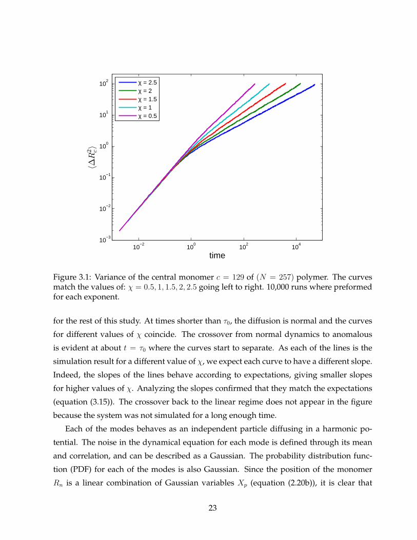
Figure 3.1 illustrates the motion of the central monomer in a polymer of size N = 257.
The location of monomer c = 129 with respect to the starting location was squared and
averaged over 10,000 independent simulations. The horizontal axis is in the characteristic
time units τ0, while the vertical axis is in units of b2. These are the units we will work with
22
10−2
100
102
104
10−3
10−2
10−1
100
101
102
time
〈∆R
2 c〉
χ = 2.5χ = 2χ = 1.5χ = 1χ = 0.5
Figure 3.1: Variance of the central monomer c = 129 of (N = 257) polymer. The curvesmatch the values of: χ = 0.5, 1, 1.5, 2, 2.5 going left to right. 10,000 runs where preformedfor each exponent.
for the rest of this study. At times shorter than τ0, the diffusion is normal and the curves
for different values of χ coincide. The crossover from normal dynamics to anomalous
is evident at about t = τ0 where the curves start to separate. As each of the lines is the
simulation result for a different value of χ, we expect each curve to have a different slope.
Indeed, the slopes of the lines behave according to expectations, giving smaller slopes
for higher values of χ. Analyzing the slopes confirmed that they match the expectations
(equation (3.15)). The crossover back to the linear regime does not appear in the figure
because the system was not simulated for a long enough time.
Each of the modes behaves as an independent particle diffusing in a harmonic po-
tential. The noise in the dynamical equation for each mode is defined through its mean
and correlation, and can be described as a Gaussian. The probability distribution func-
tion (PDF) for each of the modes is also Gaussian. Since the position of the monomer
Rn is a linear combination of Gaussian variables Xp (equation (2.20b)), it is clear that
23

its motion can also be described by a Gaussian process (this property of Gaussian pro-
cesses is known from the Cramer’s theorem [31]). At very short times, the variance of the
monomer’s PDF will be linear with time, as the mean square displacement is linear. In the
anomalous regime, we know that the variance of the PDF has an anomalous dependence
on time σ2 ∝ tα (σ2 = 〈∆R2n〉). The PDF can be described by a Gaussian of the form
P (x, t) ∝ e− (x−x0)2
const b2−2α(D0t)α , (3.16)
where x0 is the initial position of the monomer. The variance in the anomalous regime
can also be calculated analytically through a sum of the variances of modes [32]. At times
larger than the τN , the variance also depends linearly on time, but with Dcm.
Anomalous processes have many unique features. The behavior when adding differ-
ent boundaries condition differs dramatically from that of a single particle. Studying our
model in the presence of one and two absorbing boundaries, we analyze the spatial prob-
ability density function and the absorption time probability density, and compare them
to the results of other models.
24

Chapter 4
Tagged monomer dynamics in the
presence of absorbing boundaries
4.1 Absorption time in the presence of two boundaries
First passage time (FPT) problems arise in many areas of physics where stochastic behav-
ior is observed. In its simplest form it describes a Brownian particle that diffuses until it
reaches a certain reactive site and a reaction takes place. More complex situations involve
many reaction sites and interaction between particles. Typical examples of FPT processes
are fluorescence quenching and neuron firing, or the purchase and sale of stocks when
their value reaches a certain price [33]. The common property to all these processes is
their termination when a certain value is reached. For many problems, the first passage
phenomenon is modeled by the first passage probability Q (t). This is the probability that
a process was terminated at time t. In the case of a random walker, this is the proba-
bility that the walker hits a boundary for the first time at t. When the particle reaches
the boundary, it disappears and the process stops. In terms of boundary condition, stop-
ping the process when a certain point is reached is equivalent to placing an absorbing
boundary condition at that point. First passage time and absorption processes are in fact,
mathematically identical. We can also define the probability that a diffusing particle has
25

not yet hit the absorbing boundary at time t as its survival probability S (t). The connec-
tion between the two quantities is given by
S (t) = 1−∫ t
0
Q (t′) dt′. (4.1)
The problem of a single diffusing particle in the presence of one or two absorbing
boundaries can be solved analytically. Their solution are discussed in details by Chan-
drasekhar [34] and in [33]. I will review them here briefly.
Consider a particle starting from position x0 = 0 at time zero. The diffusion equation
for the probability density is
∂P (x, t)
∂t= D
∂2P (x, t)
∂x2. (4.2)
For absorbing boundaries located at Xb1 = −L/2 and Xb2 = L/2, the solution is subjected
to boundary conditions P (−L/2, t) = P (L/2, t) = 0. The solution of equation (4.2) may
be written as the eigenfunction expansion of the operator at the right side of the equation,
and a time dependent part
P (x, t) =∞∑
n=0
An cos
((2n+ 1) πx
L
)e−( (2n+1)π
L )2Dt, (4.3)
where An are determined by the initial conditions. Each of the eigenfunctions decays
exponentially with a different relaxation time given by τn = L2
(2n+1)2π2D. At long times, only
the slowest eigenfunction survives and P (x, t) = A1 cos(
πxL
)e−( π
L)2Dt. The relaxation time
τ1 = L2/π2D of the slowest mode is of the order of the characteristic time for diffusing the
length of the interval between the walls. As a result, the asymptotic survival probability
decays as
S (t) ∝ e−( πL)
2Dt ≡ e−t/τ1 . (4.4)
The first passage time distribution can be characterized by its moments and the mean
time to hit or exit the boundaries. The n-th moment of the distribution is given by
〈tn〉 =
∫ ∞
0
tnQ (t) dt. (4.5)
The characteristic time scale for the first passage problems is L2/D. For example, in the
problem of a diffusing particle between two walls, the mean passage time is just τ =
26

0 1000 2000 3000 4000 5000 6000 700010
−6
10−5
10−4
10−3
10−2
time
prob
abili
ty d
ensi
ty
2571296533951
Figure 4.1: Probability distribution of the absorption time of the central monomer ofGaussian (χ = 2) polymers of lengths N = 1, 5, 9, 33, 65, 129, 257 (plotted left to right).Two absorbing boundaries are present at Xb1 = −8 and Xb2 = 8. For each polymerlength, 100,000 independent runs were preformed.
L2/8D. When the particle starts its motion near the center of the interval, the moments of
the first passage time behave as 〈tk〉 ∝ (L2/D)k.
First passage time problems with anomalous diffusion have been studied extensively.
Most models use Levy type diffusion or the FDE to study the FPT distributions.
The dynamics of a tagged monomer in a polymer can be treated analytically, as we
have shown in the previous chapters. However, the treatment cannot be extended to
include absorbing boundaries. Although the equation for the monomer motion can be
separated to independent Langevin equations for the modes, the introduction of bound-
aries in the real space couples the equations again. We use numerical methods to study
the behavior of our model system in the presence of boundaries.
Let us introduce absorbing boundaries into our model system. We simulated the dy-
namics of Gaussian polymers (χ = 2) of different lengths (N = 2l + 1 where l is a natural
27

number) by solving equation (3.9) numerically using the SMC method. At every time
step, we followed the motion of the central monomer (c = 2l−1 + 1) by transforming the
modes amplitudes to the real space (equation (2.20b)) and checking if it had crossed the
boundaries, i.e. has been absorbed. At t = 0, we located c at the origin while the entire
polymer was at equilibrium and placed absorbing boundaries at Xb1 = −8 and Xb2 = 8.
Figure 4.1 depicts the probability distribution of the absorption time (denote Q (t)) on a
semi-log scale. We can see that for small polymers, the distribution is similar to that of a
single particle with a diffusion constant of Dcm = D0/N . This happens because, for small
polymers, the radius of gyration is smaller than the length of the interval and the slow-
est relaxation time is smaller than the time it takes to diffuse the interval with the Dcm.
The probability distribution of the absorption time for a single particle can be derived
from equation (4.3) with the matching initial conditions. From the equation, it is clear
that, for long times, the probability function decays exponentially with a time constant of
τ ≈ X2b /2Dcm.
As we take longer polymers, the distributions start to coincide, until they overlap for
polymers of lengths N = 65, 129, 257. This occurs because, for large polymers, the radius
of gyration is larger than the boundary size and the longest relaxation mode exceeds the
mean absorption time. For N = 257 for example, the slowest relaxation time is τ1 ≈1.3 × 10⁴, while the characteristic time to diffuse the interval with anomalous exponent
α = 1/2 is X4b /b
2D0 ≈ 4 × 10³. Because in this regime the distribution function becomes
independent of the polymer size, we are guaranteed that the monomer’s motion will be
anomalous even at long times. This can also be observed in figure 3.1, where the diffusion
is anomalous throughout the entire process.
Note that the asymptotic behavior of the absorption time distribution in figure 4.1 is
clearly an exponential decay. This excludes the possibility of describing the distribution
as a stretched exponential ln (Q (t)) ≈ −t1/2(D/X2b )1/2 at large times, as was previously
proposed by Nechaev et al. [35].
Now let us see how the shape of the absorption time distribution function changes as
we change the anomalous exponent. To do so, we simulated equation (3.9) with differ-
ent values of χ, each produces a different exponent according to equation (3.15). Again,
at the beginning of each simulation, monomer number 129 of an equilibrated polymer
(N = 257) was placed at the origin and its location was followed in time. In figure 4.2, we
28

0 1000 2000 3000 4000 5000 6000 7000
10−4
10−3
10−2
time
prob
abili
ty d
ensi
ty
χ=2.5χ=2χ=1.5χ=1χ=0.5
Figure 4.2: Probability density for the absorption times of a central monomer in aN = 257polymer, in the presence of two absorbing boundaries set at Xb1 = −8 and Xb2 = 8. Eachof the curves is the result of 100,000 independent simulation with a certain χ. The differentcurves correspond (from left to right) to χ = 0.5, 1, 1.5, 2, 2.5.
29

illustrate in a semi-log plot, the results of the absorption time distributions. The distribu-
tions have the same general shapes. Since at large times the curves appear to be straight
lines, it is evident that they still decay exponentially. However, the time scale, differs for
each of the curves. Because of the exponential decay, its time constant should be of the
same order as the mean absorption time. In the N -independent regime, we would expect
the constant to depend solely on the exponent and on the time scale of the problem.
Previously, it was shown by Yuste et al. [36] and Gitterman [37] that, for subdiffusion
processes described by the fractional diffusion equation, the absorption time distribution
decays in large times as a power law and that the mean time of absorption is infinite. In
our subdiffusion process, this is not the case. As the distribution decays exponentially
for large time, we are guaranteed that the distribution has a converging first moment.
Because we are in the infiniteN regime (the distribution shape has noN dependence), the
mean time can depend only on the length of the interval (the distance from the boundaries
to the initial point), the monomer’s diffusion coefficient, and the anomalous exponent.
From the equation for the mean square displacement (3.14), we expect it to be of the
order
T ≈ D−10
(L/b1−α
)2/α. (4.6)
In fact, since this is the only time scale in our problem, we expect all our characteristic
times to be of the same order. In figure 4.3 are depict three characteristic times of our
system: the exponential decay constant of the absorption time distribution, the calculated
first moment of the distribution and the theoretical time constant T as calculated from
equation (4.6) with L = 8b and D0 = b2/τ0. We plotted these times as a function of
the anomalous exponent. The decay constant and the mean absorption time give very
similar results. The difference between them results probably from the way we chose the
data points for analysis. Comparing them to T , we see that the curves behave differently
for smaller values of α, whereas for higher values the curves have similar slopes. It seems
that as α goes to 1, the curves are similar up to a constant that does not depend on the
exponent. In the same way that the characteristic time in the single particle problem
differs from the mean absorption time in a prefactor, we expected to see a difference in
our case. In principle, it is possible that the prefactor would have a certain dependence
on α. This behavior creates the different slopes for the curves.
30

Contrary to the result of the fractional diffusion equation, we get a finite mean absorp-
tion time in our subdiffusion process. This implies that if it would have been possible to
describe our model by an operator equation in the real space, it would not be the frac-
tional diffusion equation.
0.5 0.6 0.7 0.810
1
102
103
104
105
α
time
Figure 4.3: Comparison between the mean absorption time (squares) with the exponentialdecay time constant (diamonds) as calculated from the data shown in figure 4.2. Alsoshown is T (asterisks) as calculated from equation (4.6) with L = 8b and D0 = b2/τ0
31

4.2 Absorption time in the presence of one boundary
Now we turn our attention to the behavior of our model in the presence of a single ab-
sorbing boundary. We begin by reviewing the problem of a single particle performing
normal diffusion in the presence of one absorbing boundary. A detailed description can
be found in Chandrasekhar’s article [34].
Consider a particle performing normal one-dimensional diffusion starting from loca-
tion x0 > 0. An absorbing boundary located at the origin Xb = 0, sets the probability dis-
tribution function of the particle to be zero at that location. The most convenient way to
solve the differential equation with this boundary condition is using the images method.
We can place an image particle with a negative probability distribution function at the
location x = −x0 at the beginning of the process. We allowed both particles to diffuse
freely in the whole space. The addition of the image fulfills the boundary condition for
which P (x = 0, t) = 0. The probability distribution for the two particles can be written as
the sum of Gaussians of two freely diffusing particles located respectively at x0 and −x0
where the PDF of the image particle has a negative sign
P (x, t) =1√
4πDt
[e−(x−x0)2/4Dt − e−(x+x0)2/4Dt
]. (4.7)
The absorption time distribution is given by the flux at the boundary. It can be derived
from the probability distribution (4.7)
Q (t) = −D∂P (x, t)
∂x|x=0 =
x0√4πDt3
e−x20/4Dt. (4.8)
In the long time limit√Dt � x0, when the diffusion length is much bigger than the
initial distance to the boundary, the absorption time distribution behaves as a power law
Q (t) ∝ t−3/2. Because the first moment of the distribution diverges, the mean time to
reach the boundary is infinite. The first moment diverges because the distribution has a
long tail, a similar behavior to that of CTRW, where the waiting time distribution decays
as a power law.
We return now to our model. We wanted to investigate the diffusion of the tagged
monomer in the presence of a single absorbing boundary for different anomalous expo-
nents. We performed simulations in which a single absorbing boundary was placed at
Xb = −8 and the central monomer c = 129 of a polymer N = 257 was placed at the origin
32

x0 = 0 at t = 0. As we have already shown for the case of two boundaries, we are in
the infinite N regime, where the radius of gyration of the polymer is of the order of the
distance to the boundary (the same numeric estimations apply). In this regime, the poly-
mer is sure to perform anomalous diffusion throughout the process. We also performed
simulation for polymers of different lengths and saw the congruence of the absorption
time distributions for large polymers (data not shown). At very long times, unabsorbed
monomers will probably diffuse far away from the boundary, and their diffusion at this
regime would be normal. That happens when the time is considerably large than τN , and
in our simulations we do not reach this time limit.
Figure 4.4 depicts the absorption time probability distributions of the tagged monomer
for different values of χ in a logarithmic plot. Also shown is the absorption time distri-
bution of a single particle performing normal diffusion (equation (4.8)). For small values
of χ, the exponent approaches the normal diffusion limit, and we see that the probability
density resembles that of a single particle. At large times, the probability density clearly
behaves as a power law. This result can be compared to the study of Ding et al. [38],
which investigated a CTRW using the fractional Fokker-Planck equation in subdiffusion
and superdiffusion. In their study, one absorbing boundary is placed at the origin and the
other at infinity which makes it a one absorbing boundary problem. Ding et al. derived an
expression for the absorption time distribution and give an expression for its asymptotic
behavior at large times:
Q (t) ∝ t−1−α/2, (4.9)
where α is the anomalous exponent. In the case of normal diffusion where α = 1, we get
the expected power law behavior of −3/2 of equation (4.8).
In figure 4.4, we drew over the distributions, lines with the expected power law as
specified by equation (4.9). The fit between the curves and the long time behavior is
very good. While the absorption time probability density with two boundaries decayed
exponentially in the long time limit, which was in disagreement with the results of FDE,
here we see that the long time behavior matches that of FDE.
33

101
102
103
104
10−4
10−3
time
prob
abili
ty d
ensi
ty
χ=2.5χ=2χ=1.5χ=1χ=0.5N=1
Figure 4.4: Absorption time distribution of monomer c = 129 of a polymer N = 257,in the presence of an absorbing boundary at Xb = −8. The curves correspond toχ = 0.5, 1, 1.5, 2, 2.5 going left to right. For each χ value, 100,000 independent runs wereperformed. The leftmost curve corresponds to the absorption distribution of a single par-ticle performing normal diffusion under the same initial and boundary conditions. Thedotted lines give the large time approximation of the distribution corresponding to equa-tion (4.9).
34

4.3 Probability density in the presence of one absorbing
boundary
In the following chapters, we consider the probability distribution function (PDF) of the
tagged monomer position in the presence of absorbing boundaries. We begin with the
case of a single boundary.
In the previous chapter we showed that the problem of a single particle performing
normal diffusion under the influence of one absorbing boundary can be solved using the
addition of an image particle. When we have a particle performing Levy flights (which
would result in anomalous diffusion), the use of this method is more problematic. The
method of images is expected to work only when the boundary is also a turning point of
the trajectory, i.e. when the particle cannot pass the boundary without being absorbed.
In the case of LF, the particle can perform a long jump that would take it far across the
boundary. That is the reason the image method fails in this case [32, 39].
Our model is a non-Markovian process. At every time step, the monomer’s position is
the Fourier transform of the Rouse modes amplitudes. Since each of the modes changes
on a different time scale, sequential steps depend on one another. The application of
the image method assumes that steps are independent. Thus it does not work for our
subdiffusion system.
Figure 4.5 depicts the probability distribution function for the central monomer of
a Gaussian polymer (χ = 2) of length N = 257 with an absorbing boundary present
at Xb = −8. As the times in which we simulate are short then τN , we are guaranteed
anomalous dynamics throughout the process. At the beginning of the simulation, the
tagged monomer was placed at the origin and the polymer was equilibrated. The shape
of the PDF is quite different from that of a single particle (equation (4.7)) performing
normal diffusion. The PDF of a single particle is linear near the boundary, while the
distribution in the figure is clearly not so. Thus, it is evident that the use of the image
method is not applicable here.
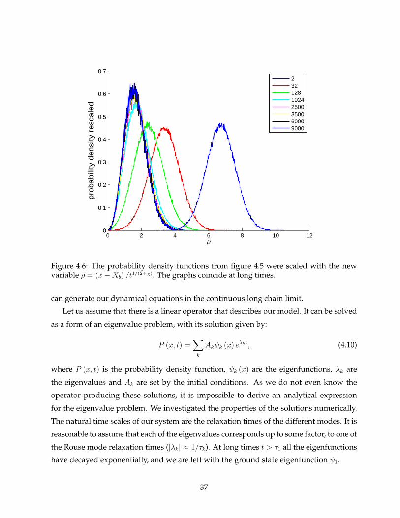
At long times, the distribution exhibits self-similarity. We can show that by rescaling
the distributions from figure 4.5. Let us introduce a new variable ρ = (x−Xb) /t1/(2+χ),
where x is the position of the tagged monomer and t is the time. The result of the scal-
ing after normalization is illustrated in figure 4.6. We can understand this behavior if
35

−5 0 5 10 15 20 25 300
0.02
0.04
0.06
0.08
0.1
0.12
0.14
0.16
0.18
0.2
x
prob
abili
ty d
ensi
ty
321281024140018002500400060009000
Figure 4.5: Probability density function of the central monomer in a polymerN = 257. Anabsorbing boundary was located at Xb = −8. The curves correspond (narrow to broad)to different times, as shown in the legend. The distribution was obtained by 100,000independent runs.
we recall the dependence of the mean square deviation on time (equation (3.14)) in the
absence of absorption and observe the shape of the PDF in the anomalous regime (equa-
tion (3.16)). Since the size√〈R2 (t)〉/t1/(2+χ) is constant, after the rescaling, the probability
density losses at long times its time dependence.
The probability density of the tagged monomer might be described as the eigenfunc-
tion of some linear operator in the real space, with corresponding boundary condition (in
our case one or two absorbing boundaries). However, our model is defined in the Fourier
space while our boundary conditions are described in the real space. From our results
so far, we know that this operator is not the FDE. We are not even sure if it is linear. We
have, however, some intuition about its origin. In the section describing the physical mo-
tivation for our model (3.1.1), we showed that the Langevin equations of Rouse model,
along with a distance-dependent interaction that couples the velocities of the monomers,
36
0 2 4 6 8 10 120
0.1
0.2
0.3
0.4
0.5
0.6
0.7
ρ
prob
abili
ty d
ensi
ty r
esca
led
23212810242500350060009000
Figure 4.6: The probability density functions from figure 4.5 were scaled with the newvariable ρ = (x−Xb) /t
1/(2+χ). The graphs coincide at long times.
can generate our dynamical equations in the continuous long chain limit.
Let us assume that there is a linear operator that describes our model. It can be solved
as a form of an eigenvalue problem, with its solution given by:
P (x, t) =∑
k
Akψk (x) eλkt, (4.10)
where P (x, t) is the probability density function, ψk (x) are the eigenfunctions, λk are
the eigenvalues and Ak are set by the initial conditions. As we do not even know the
operator producing these solutions, it is impossible to derive an analytical expression
for the eigenvalue problem. We investigated the properties of the solutions numerically.
The natural time scales of our system are the relaxation times of the different modes. It is
reasonable to assume that each of the eigenvalues corresponds up to some factor, to one of
the Rouse mode relaxation times (|λk| ≈ 1/τk). At long times t > τ1 all the eigenfunctions
have decayed exponentially, and we are left with the ground state eigenfunction ψ1.
37
10−2
10−1
100
101
10−4
10−2
100
102
104
ρ
prob
abili
ty d
ensi
ty r
esca
led
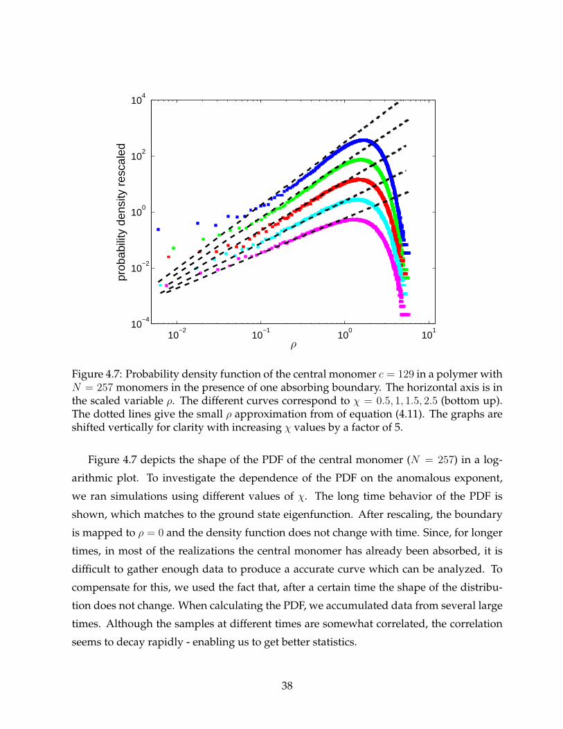
Figure 4.7: Probability density function of the central monomer c = 129 in a polymer withN = 257 monomers in the presence of one absorbing boundary. The horizontal axis is inthe scaled variable ρ. The different curves correspond to χ = 0.5, 1, 1.5, 2.5 (bottom up).The dotted lines give the small ρ approximation from of equation (4.11). The graphs areshifted vertically for clarity with increasing χ values by a factor of 5.
Figure 4.7 depicts the shape of the PDF of the central monomer (N = 257) in a log-
arithmic plot. To investigate the dependence of the PDF on the anomalous exponent,
we ran simulations using different values of χ. The long time behavior of the PDF is
shown, which matches to the ground state eigenfunction. After rescaling, the boundary
is mapped to ρ = 0 and the density function does not change with time. Since, for longer
times, in most of the realizations the central monomer has already been absorbed, it is
difficult to gather enough data to produce a accurate curve which can be analyzed. To
compensate for this, we used the fact that, after a certain time the shape of the distribu-
tion does not change. When calculating the PDF, we accumulated data from several large
times. Although the samples at different times are somewhat correlated, the correlation
seems to decay rapidly - enabling us to get better statistics.
38

Other works on anomalous diffusion in the presence of absorbing boundaries have
calculated the PDF of their process [40]. The PDFs of Levy flights and Levy walks are
usually sharply peaked, described by Fox functions [1] and look very different from the
Gaussian probability distribution of the normal Brownian motion. In the study of Zu-
mofen and Klafter of Levy walks with a single absorbing boundary [41], the PDF near
the boundary is shown both analytically and numerically to behave as a power law. Our
results show that for small ρ, the PDF converges to the power law:
P (ρ) ∝ ρ(2+χ)/2 = ρ1/α. (4.11)
This is the same scaling dependence on the anomalous exponent that Zumofen and Klafter
found in their study. This also corresponds to the linear behavior of the PDF in the case
of normal diffusion with one absorbing boundary (for α = 1). The predicted scaling of ρ
by equation (4.11) is shown in the figure as dashed lines. The simulation results indicate
(figure 4.7) that the convergence towards the power law behavior near the boundary is
slow for small ρ. Also, note that the convergence is faster for smaller values of χ. Very
close to the boundary, the results should be handled with care. We performed our simu-
lations with a finite time step, which in turn determines the mean size of the monomers’
step. At distances from the boundary of the order of the step size, the discrete nature of
the stepping mechanism emerges. For example, although we know that the PDF should
be exactly zero at the boundary, we can see in the figure that this is not the case. For this
reason, data points very close to the boundary should be ignored.
4.4 Probability density in the presence of two absorbing
boundaries
Next we consider the behavior of the central monomer of a polymer between two absorb-
ing boundaries. Figure 4.8 illustrates the probability distribution of the central monomer
of a Gaussian polymer (χ = 2) with N = 257 in the presence of two absorbing boundaries
located at Xb1 = −8 and Xb2 = 8. In the figure, we see the evolution of the distribution
in time. At very short times (t� τ0), the particle’s distribution is Gaussian with the vari-
ance σ2 ∝ t. Later on, at times considerably shorter than the mean time of absorption,
39

−8 −6 −4 −2 0 2 4 6 80
0.05
0.1
0.15
0.2
0.25
0.3
0.35
0.4
x
prob
abili
ty d
ensi
ty
283212851210241400
Figure 4.8: Probability density function of the central monomer in a Gaussian polymerwith N = 257 monomers in the presence of two absorbing boundaries at Xb = ±8. Thedistribution is shown at different times t = 2, 8, 32, 128, 512, 1024, 1400 (narrow to broad).The distribution was obtained by 100,000 independent runs.
the particle is still unaware of the presence of the boundaries and performs anomalous
diffusion with Gaussian distribution with σ2 ∝ t1/2. Analogously to equation (4.10), it
appears that at long times, only the slowest ”eigenmode” survives and the shape of the
normalized PDF stabilizes. In the long-time solution for normal diffusion (equation (4.3)),
the slowest mode is a cosine with a period twice the length of the distance between the
boundaries. This is clearly not the shape of the curve in the figure. It is also not a Gaus-
sian (as the Gaussian value is never zero). Actually, we cannot describe the distribution
with an analytical expression.
The method of images can be used to find the PDF of a normal diffuser between two
absorbing boundaries using an infinite number of images farther and farther from the
origin. The contributions of the additional images become progressively smaller and the
PDF converge to a steady form. We cannot solve the non-Markovian motion of the tagged
40

−8 −6 −4 −2 0 2 4 6 80
0.02
0.04
0.06
0.08
0.1
0.12
0.14
x
prob
abili
ty d
ensi
ty
SimulationImage method
Figure 4.9: PDF for the central monomer in a N = 257 Gaussian polymer with absorbingboundaries (blue) compared with a PDF obtained by the image method with the samevariance. Note that the graphs do not coincide.
monomer with this method. In figure 4.9 we present the long-time stable shape of the PDF
from figure 4.8 and the PDF calculated by the method of images. To produce it, we placed
particles at with a positive sign PDF at x = 0, 32,−32 and particles with negative sign PDF
at x = 16,−16. The PDF of each particle was a Gaussian with the mean value set to be the
position of the particle and variance of 1. We summed the Gaussian of all the particles.
Since the PDF converges rapidly, no additional images were needed. To compare the two
distributions, we changed the variance of the image distribution so that it would match
that of the distribution obtained from the simulations and normalized it. We can see that
the two curves do not match. The behavior of the image distribution is linear near the
boundaries while the tagged monomer’s distribution is not. This proves that, indeed, the
method of images fails to solve our problem.
Next, we investigate the behavior of the probability density as χ is changed. Figure
4.10 depicts the shape of the ”ground state eigenfunction” PDF of the central monomer
41

−8 −6 −4 −2 0 2 4 6 80
0.02
0.04
0.06
0.08
0.1
0.12
0.14
0.16
x
prob
abili
ty d
ensi
ty
χ=2.5χ=2χ=1.5χ=1χ=0.5
Figure 4.10: Probability density function of the central monomer in a polymer with N =257 monomers with absorbing boundaries at Xb = ±8, for χ = 0.5, 1, 1.5, 2.5 (bottom up).Each graph is the product of 100,000 independent runs.
in a polymer N = 257, for different values of χ. The limiting behavior of χ → 0 is that of
a single particle - the PDF becomes the cosine function. In the other limit of χ → ∞ the
distribution will give us a delta function.
Although we cannot get a closed analytical expression for the PDF, other studies that
investigated the probability density function of anomalous processes showed that, near
the boundaries, the PDF behaves like a power law. Zoia et al. [32], investigated the diffu-
sion equation with a fractional Laplacian with two absorbing boundaries. The operator
was implemented in such a way that its eigenfunction and eigenvalue could be calculated
numerically. Specifically, the shape of the long time eigenmode was found. Analysis of
the function’s behavior near the boundaries demonstrated that it has a power law depen-
dence in the anomalous exponent α
ψ1 ≈ (x−Xb1)1/α . (4.12)
42

Again, the power law behavior is the same as in the case of a single boundary condi-
tion (equation (4.11)). The Laplacian operator can be represented as a Toeplitz symmetri-
cal matrix. It was shown analytically, based on Widom’s study on the eigen-problem in
Toeplitz matrix [42], that in the limit of α→ 0, the first eigenfunction can be approximated
near the boundaries as
ψ1 ≈Γ (3/2 + 2/α)
Γ (1 + 2/α)
((x
Xb1
)2
− 1
)1/α
, (4.13)
which is consistent with the numerical result in equation (4.12).
Figure 4.11 illustrates the distribution from figure 4.10 on a logarithmic plot with the
horizontal axis shifted by −Xb1. The PDF near the boundary behaves as
P (x) ≈ (x−Xb1)(2+χ)/2 , (4.14)
which displays the same power law behavior near the boundary as equation (4.12). Also
shown are dashed lines fitted to each distribution, corresponding to x(2+χ)/2. Very near
the boundary, the distributions deviate from the expected power law and converge to the
small x approximation farther along the axis. Note that the convergence for the power
law is faster to for smaller values of χ, while for χ = 2.5 the convergence is rather poor.
In our simulations, we produced different probability distributions for different val-
ues of χ. We wanted to find out if a distribution for a specific χ can actually be calculated
from the solution for another χ by some change of variables or a rescaling of some kind.
Through algebraic analysis of the dynamical equations (3.9), one can see that it is not pos-
sible to define an effective time variable, such that χwill be scaled out of all the equations.
By analyzing the distribution in figure 4.10, we can also show that the distribution for one
χ cannot be calculated from that of another. Based on the small x approximation (equa-
tion (4.14)), we wanted to match the power law behavior of all the distribution to that of
the distribution for the Gaussian polymer (χ = 2). We raised all the other distributions
to the power of 4(2+χ)
and normalized them. The result is presented in figure 4.12. We
see that the distribution are similar but they do not collapse. This indicates that the pro-
cess is unique for every χ in the same way the eigenfunctions in the fractional Laplacian
problem are unique for every α.
43

10−1
100
101
10−3
10−2
10−1
100
101
102
x-xb1
prob
abili
ty d
ensi
ty
Figure 4.11: Probability density function of the central monomer in a polymer with N =257 in the presence of absorbing boundaries atXb1 = −8 andXb2 = 8, for χ = 0.5, 1, 1.5, 2.5(bottom to top). The dashed lines give the small x approximation x(2+χ)/2. Each curve isthe product of 100,000 independent runs. The curves are shifted vertically for clarity withincreasing χ values by a factor of 5.
44

−8 −6 −4 −2 0 2 4 6 80
0.02
0.04
0.06
0.08
0.1
0.12
0.14
x
prob
abili
ty d
ensi
ty r
esca
led
χ=2.5χ=2χ=1.5χ=1χ=0.5
Figure 4.12: The probability densities from figure 4.10 were rescaled to match the PDF forχ = 2 by raising each of them to the power of 4
(2+χ)to match them in the small x approx-
imation of equation (4.14). Note that the curves do not collapse, thus demonstrating thatthe solution for each χ is unique and can not be calculated from that of another.
45

Chapter 5
Translocation
In this chapter we will discuss the similarities between the system of a tagged monomer
in the presence of two absorbing boundaries and translocation. We begin by reviewing
the translocation process.
There are many biological systems in which a polymer diffuses or is pulled through
a pore in the lipid membrane of the cell. This process is known as translocation. Phages,
for example, invade bacteria by taking advantage of existing channels in bacterial mem-
brane and translocate their DNA through it [43]. Inside the cell, peptides translocate into
organelles by specific channels. Lately, translocation has drawn much attention as a po-
tential method to sequence DNA (read its nucleotide sequence). Deamer et al. [44, 45]
introduced an experimental method for rapid DNA sequencing. The DNA is threaded
through a bacterial channel (alpha-hemolysin) and the nucleotide residing in the pore
can be identified by measuring the ionic current through the channel. This new method,
though promising, still lacks the proper resolution to sequence DNA correctly.
A number of theoretical and numerical works have shed light on the translocation
process. A common approach is to describe the dynamics of the process through a single
dynamical variable which is the number of the monomer currently inside the pore. This
variable is known as the translocation coordinate (denoted s (t)). The translocation is
completed when the translocation coordinate is 0 or N + 1, i.e. when the polymer has left
the pore. As the polymer is threaded through the pore, it faces an entropic barrier [46].
Since the number of possible configurations is least when the polymer is halfway through
the pore, the polymer has to surmount the barrier in order to complete its translocation.
46
Early works modeled the translocation process as a form of Brownian dynamics [47].
The process was described by the diffusion equation with s (t) as the dynamical variable.
In this formalism, the process resembles the diffusion of a particle between two absorbing
boundaries. This Brownian model constitutes the mean translocation time to scale with
the polymer’s length N as N2. However, it was argued by Kantor et al. [9], that the
translocation cannot be faster than the relaxation time that scales as Nα, where α = 1+2ν
is larger than two, for a self-avoiding polymer performing Rouse dynamics. The slowest
relaxation time is of the order of the time it takes for a polymer to diffuse its own radius of
gyration and it is not reasonable to assume that the constraint of a pore would accelerate
the process rather then slowing it down. The relaxation time sets an lower bound on the
mean translocation time. The result was also corroborated by Monte Carlo simulations.
Recent simulations in 3D have argued that the translocation is even slower [48], but the
validity of these results has yet to be proven [49].
It is not clear what kind of equation would best describe the translocation process. It
was argued [50] that it can be described by a fractional diffusion equation. This would
result in an infinite mean translocation time. However, experiments and numerical stud-
ies indicate that the mean translocation time is well defined. Since our model also gave
finite mean time of absorption for the case of two absorbing boundaries, it is reasonable
to compare it with the translocation process.
The translocation process and the dynamics of a tagged monomer between two ab-
sorbing boundaries have certain similarities. In both processes, we follow the dynamics
of a single dynamical variable - the translocation coordinate s (t) and the position of the
tagged monomerRn (t). In both cases, the variable performs anomalous diffusion because
of its interactions with the other monomers, and its dynamics is governed by Rouse re-
laxation. While the tagged monomer diffuses in the real space until it is absorbed by one
of the boundaries, the translocation coordinate diffuses in the discrete monomer number
(index) space (1...N ) until one of its edges has diffused out of the pore and the polymer
has fully translocated.
We decided to study the analogies between the processes by comparing their proba-
bility distribution functions. Simple scaling considerations [9, 51] suggest that the mean
square displacement of the reaction coordinate scales with time as 〈∆ (s (t))2〉 ∝ tα with
α = 2/ (1 + 2ν) which is 0.8 in 2D.
47

We compared the PDF of the translocation coordinate of a 2D self-avoiding polymer
of size N = 128 (data from Chatelain et al. [52]) with the PDF of the tagged monomer
location as obtained from our model with χ = 0.5 for the central monomer of polymer
N = 257 (figure 4.10). As the two processes have the same anomalous exponent α = 0.8,
they are comparable. The result is presented in figure 5.1. The two dynamical variables
were rescaled to x ∈ [0, 1] for the purpose of comparison. Both distributions were ob-
tained after a long time (with respect to the mean passage time). At this point in time,
only the ”slowest eigenmode” survived. The translocation PDF was obtained by a Monte
Carlo simulation on a 2D lattice. The absorption time distribution indicated an exponen-
tial decay as does our model. Since, at long times, most of the polymers have already
translocated, the statistics for the results are not very good.
We can see that the curves are mostly congruent. The main difference between them
occurs near the boundaries where the function is expected to go to zero as a power law
with an exponent of 1.25 (equation (4.14)). However, the translocation PDF decreases
faster, with a power of ≈ 1.44 [52]. The logarithmic plot, in figure 5.2 shows that, the PDF
produced by our model converges to the expected exponent, while the translocation PDF
does not.
The high resemblance between the functions is promising. It is clear that the processes
share many features. The translocation problem is still under debate in the scientific com-
munity. More and more complex simulations are being performed to investigate the de-
pendence of the mean translocation time on the polymer length and relaxation dynamics
of the polymers. Yet, no single equation which could describe it sufficiently well was
found. Models such as ours might hint on some of the features of a future solution.
48

0 0.2 0.4 0.6 0.8 10
0.2
0.4
0.6
0.8
1
1.2
1.4
1.6
1.8
x
prob
abili
ty d
ensi
ty
Figure 5.1: Probability density function of the central monomer in a polymer N = 257monomers with χ = 0.5 from figure 4.10 (ragged line). Probability density function ofthe translocation coordinate of a translocating polymer N = 128 (smooth line with cir-cles). The data was taken from [52]). The two PDF’s were shifted to x ∈ [0, 1] to enablecomparison.
49

10−3
10−2
10−1
100
10−3
10−2
10−1
100
x
prob
abili
ty d
ensi
ty
Figure 5.2: The same graphs as in figure 5.1 on logarithmic scale. The ragged line is theresult of the our simulation with χ = 0.5, while the smooth line with circles is the translo-cation PDF. Also shown (dashed line) is the power law behavior near the boundaries withexponent of 1.25.
50

Chapter 6
Conclusion
We have investigated the anomalous motion of a tagged monomer in a polymer. We ex-
amined the effect of a monomer-coupling interaction on the Rouse model. The interaction
couples the motion of the monomers through their velocities, much like the hydrodynam-
ical interaction, and its strength decays with distance between them as a power law with
exponent χ. As it turned out, the addition of the interaction (under certain approxima-
tions) leads to the mean square displacement of the tagged monomer depending on time
as 〈∆Rn (t)2〉 ∝ tα with α = 2/ (2 + χ). This motivated us to define a model in the Rouse
(Fourier) space, that produces anomalous behavior of the tagged monomer with expo-
nent α. The ability to control the exponent χ, enables us to get any subdiffusion exponent
we desire. While most standard models used to investigate anomalous diffusion are mo-
tivated by mathematical concepts (fractional derivatives, for example), we developed a
physical model which can be used to investigate subdiffusion processes. The dynamics of
the monomers can be described in the Rouse space, where each mode changes on a differ-
ent time scale depending on χ. From this dependence, the anomalous behavior emerges
when transforming back to the monomer space.
Using simulation methods, we investigated the dynamics of the monomer in the pres-
ence of one and two absorbing boundaries, and found the absorption time distributions
and the probability density functions. For one absorbing boundary, our model resem-
bles the long-time behavior of absorption time distributions of other models. The power
law tail in our model and its dependence on the anomalous exponent are similar to those
found in other subdiffusion models (CTRW and fractional diffusion equation). For two
51

absorbing boundaries, our distribution decays exponentially in the long-time regime, and
its decay time constant depends on the anomalous exponent. The time distribution has a
finite mean, while, in fractional diffusion equation models and Levy flights, the distribu-
tion has a power law tail and the mean time diverges.
We have also shown that the behavior of the PDF of the tagged monomer’s position
is similar to the known shape of PDF in other models. Near the boundaries, the PDF is
expected to behave as a power law with an exponent of 1/α (where α is the anomalous
exponent). In our results, both for one and two boundaries, the PDF converges to the
expected exponent, whereas the convergence is faster for smaller values of χ.
The translocation process shares many features with our model. We compared the
PDF of the position of the tagged monomer with χ = 0.5 to that of the translocation coor-
dinate of a self avoiding polymer in 2D. The two curves are very similar in shape, but they
differ in their behavior near the boundaries. In fact, the two processes are quite different
in nature. Our polymer is equilibrated at all times, while the translocating polymer, in
a way, is never at equilibrium. A process at equilibrium travels at all times through the
same phase space. Yet, because the phase space in the translocation process is determined
by the length of the strand on each side of the pore, the passage of a monomer changes
it. It seems that our model cannot describe translocation precisely, as their probability
distributions differ from one another. Nonetheless, perhaps it can suggest the structure
of a future model that could give an exact description of translocation.
52

Appendix A
Treatment of polymer dynamics
A.1 The discrete cosine (Fourier) transform
Rouse equations can be decoupled by transforming them to the Fourier space. In our
model, we work with a discrete polymer, composed ofN monomers. In the Rouse model,
the dynamics of each monomer is described by the Langevin equation. For the equations
for the end monomers, n = 1 and N (2.17), to resemble those for the other monomers
(2.16), we define additional hypothetical monomers
R0 = R1 (A.1)
RN+1 = RN . (A.2)
We use the discrete cosine transform (DCT ) [53] which fulfills the condition on the
end monomers
Xp =1
N
N∑n=1
Rn cos
(n− 1
2
)pπ
N, (A.3a)
Rn = X0 + 2N−1∑p=1
Xp cos
(n− 1
2
)pπ
N, (A.3b)
where the set of mode functions are
cos
(n− 1
2
)pπ
Nn = 1, ..., N, p = 1, ..., N − 1. (A.4)
We show that the functions form an orthogonal set. First let us find the following sum
Sn(θ) ≡n+1∑k=1
cos
(k − 1
2
)θ. (A.5)
53

We will solve it by using complex variable
eiθ/2(1 + eiθ + ...+ einθ
)= exp
(iθ (n+ 1)
2
) sin(
θ(n+1)2
)sin(
θ2
) .
After taking the real part of the above relation
Sn(θ) =sin(θ(n+ 1))
2 sin(
θ2
) . (A.6)
We note that {Sn(θp) = 0 , for θp = pπ
n+1, and
Sn(0) = n+ 1.
The inner product Clm of two functions cos(lθk) and cos(mθk)
Clm =n+1∑k=1
cos(lθk) cos(mθk) =1
2
n+1∑k=1
[cos(l +m)θk + cos(l −m)θk] =
1
2
[Sn(
(l +m)π
n+ 1) + Sn(
(l −m)π
n+ 1)
].
From this we get the functions orthogonality relation:
Clm =1
2(n+ 1)δl,m (A.7a)
C00 = n+ 1 (A.7b)
A.2 Langevin equation of Rouse modes
The one-dimensional over-damped Langevin equation for the location x of a particle,
under the influence of an external potential U and a random force f is of the form
dx
dt= −∂U
∂x+ f. (A.8)
In the Rouse model, a polymer is described as a chain of monomers connected by har-
monic springs. The Hamiltonian for N monomers is given by
H =κ
2
N−1∑n=1
(Rn −Rn+1)2. (A.9)
54

The Langevin equation for monomer n, influenced by the Hamiltonian is:
ζdRn
dt= −κ(2Rn −Rn+1 −Rn−1) + fn (A.10)
with the noise defined as:
〈fn(t)〉 = 0 (A.11a)
〈fn(t)fm(t′)〉 = 2ζkBTδn,mδ(t− t′). (A.11b)
We use a white noise with zero mean and a correlation which depends on the friction
constant. The Fourier and inverse Fourier transform of the random noise are respectively
given by
fp =1
N
N∑n=1
fn cos(n− 1
2)pπ
N(A.12a)
fn = f0 + 2N−1∑p=1
fp cos(n− 1
2)pπ
N. (A.12b)
Now we can present the Langevin equation (A.10) in Fourier space by inserting the
Fourier transform of the variables:
ζ
[dX0
dt+ 2
N−1∑p=1
dXp
dtcos(n− 1
2)pπ
N
]= −κ
[4
N−1∑p=1
Xp cos(n− 1
2)pπ
N− 2
N−1∑p=1
Xp cos(n+1
2)pπ
N
− 2N−1∑p=1
Xp cos(n− 3
2)pπ
N
]+ f0 + 2
N−1∑p=1
fp cos(n− 1
2)pπ
N.
Because the mode functions are orthogonal, the equality in the above expression holds
for every value of p. The equation for each mode (multiplied by N ) is
2ζNdXp
dt= −8Nκ sin2
( pπ2N
)Xp + 2Nfp, (A.13)
The noise correlation in Fourier space is given by:
〈fp(t)fp′(t′)〉 =
1
N2
∑mn
cos(n− 1
2)pπ
Ncos(m− 1
2)p′π
N〈fn(t)fm(t′)〉 =
1
N2
∑n
cos(n− 1
2)pπ
Ncos(n− 1
2)p′π
N2ζkBT.
55

By using (A.7) we get
〈fp(t)fp′(t′)〉 = 2ζkBTδp,p′δ(t− t′)
1
2N, p = 1, 2, ..., N − 1, (A.14)
〈f0(t)f0(t′)〉 = 2ζkBTδ(t− t′)
1
N. (A.15)
If we define Wp = 2Nfp, equation (A.13) can be rewritten as
ζpdXp
dt= −κpXp +Wp, (A.16)
where ζp = 2ζN , and ζ0 = ζN . The random variable Wp is now characterized by
〈Wp (t)〉 = 0, (A.17a)
〈Wp (t)Wp′ (t′)〉 = 2kBTζpδp,p′δ(t− t′). (A.17b)
Equation (A.16) of each mode (p ≥ 1) is the equation for a particle in an harmonic
potential with noise. The modes relax with the characteristic time
τq =ζqκq
=ζ
12kBT
[b
sin2( q2)
]2
. (A.18)
The Hamiltonian for the model can also be written in terms of Rouse modes. In the
Rouse space, the Hamiltonian is written as the sum of energies from N − 1 independent
harmonic springs, each with a different spring constant
H =
π(N−1)N∑
q= πN
1
2κqX
2q . (A.19)
56

A.3 Solution of Langevin equation in harmonic potential
Here we give some analytical results for Langevin equation of a particle in harmonic
potential.dx
dt= −κx+ f, (A.20)
with the noise moments given in equation (A.11).
First we find the correlation between the value of x (t) and its initial value x(0):
〈x(t)x(0)〉 =1
ζ2
∫ t
−∞dt1
∫ 0
−∞dt2 exp
[−(t− t1 − t2)
τ
]〈f(t1)f(t2)〉
=1
ζ
∫ t
−∞dt1
∫ 0
−∞dt2 exp
[−(t− t1 − t2)
τ
]2kBTδ(t1 − t2)
=kBT
κexp(−t/τ)
Note that the equilibrium properties are independent on the friction constant ζ , and that
the correlation decays exponentially with the characteristic relaxation time τ = ζ/κ.
The first moment and variance of the random variable x can also be calculated
x(t) = x(0) exp(−t/τ) +1
ζ
∫ t
0
dt′ exp (−(t− t′)/τ) f (t′) (A.21)
〈x(t)〉 = x(0) exp(−t/τ) (A.22)
〈(x(t)− 〈x(t)〉)2〉 =1
ζ2
∫ t
0
dt1
∫ t
0
dt2 exp (−(t− t1 + t− t2)/τ) 〈f(t1)f(t2)〉
=1
ζ
∫ t
0
dt1 exp [−2(t− t1)/τ ] 2kBT =kBT
κ[1− exp(−2t/τ)] (A.23)
Equation (A.23) describes the relaxation of the variance of a mode.
A.4 Approximate treatment of velocity-dependent interac-
tion between monomers
In this section, we describe the physical motivation that led us to define our model.
The Rouse model can be generalized by adding a long distance interaction. Since the
monomers diffuse in a solvent, their movement results in a force on their nearby solvent
known as the hydrodynamical interaction. The interaction couples the velocities of the
57

monomers. To include them into a the Rouse model, the monomer’s Langevin equation
is rewritten with a mobility tensor. The strength the hydrodynamical interaction decays
with the monomer distance as |Rn −Rm|−1 [12]. Let us introduce an interaction whose
strength decays as a power law with the exponent χ. The corresponding mobility matrix
describing it is given by
Onm =
I/ζ n = m
bχ
ζ|Rn−Rm|χ [I + rnmrnm] n 6= m,(A.24)
where rnm is a unit vector in the direction of Rn − Rm. For one dimension, the expres-
sion for n 6= m is reduced to bχ
ζ|Rn−Rm|χ . The generalized Langevin equation for the n-th
monomer is written as:
∂
∂tRn =
∑m
Onm
(− ∂U
∂Rm
+ fm(t)
). (A.25)
To solve this equation, we would need to simplify it. An approach previously taken by
Kirkwood [29] for hydrodynamical interaction, was to approximate the mobility matrix
by its average equilibrium value (this operation is call preaveraging). In our case, we can
use the equilibrium distribution of the monomer-monomer distance Φeq to find the value
of Onm over all possible monomers realizations.
Onm → 〈Onm〉 =
∫d{Rn}OnmΦeq{Rn}. (A.26)
To calculate it, we insert the distribution function (2.9). Since the distribution of rnm is
independent of |Rn −Rm|, the average interaction can be written as
〈Onm〉 =bχ
ζ
⟨1
|Rn −Rm|χ⟩〈[I + rnmrnm]〉 . (A.27)
Using 〈rnmrnm〉 = Id, we have
〈Onm〉 =bχI (d+ 1)
ζ d
⟨1
|Rn −Rm|
⟩, (A.28)
where d is the dimensionality.
〈Onm〉 =
∫ ∞
0
dr2πd/2
Γ (d/2)rd−1
(d
2π |n−m| b
)d/2
exp
(− dr2
2 |n−m| b2
)(d+ 1) bχ
d ζrχ=
=2 (d+ 1)
Γ (d/2) d
(d
2 |n−m|
)χ/21
ζ
∫ ∞
0
td−1−χ exp(−t2)dt ≡ h (n−m) .
58
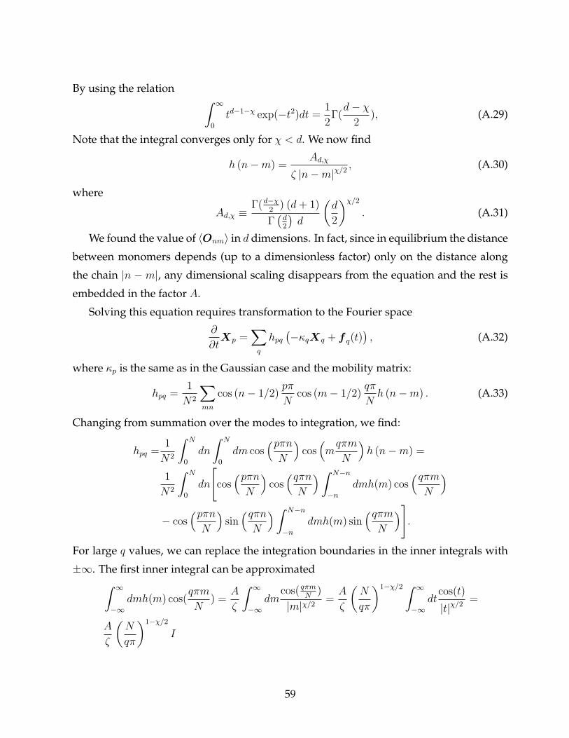
By using the relation ∫ ∞
0
td−1−χ exp(−t2)dt =1
2Γ(d− χ
2), (A.29)
Note that the integral converges only for χ < d. We now find
h (n−m) =Ad,χ
ζ |n−m|χ/2, (A.30)
where
Ad,χ ≡Γ(d−χ
2) (d+ 1)
Γ(
d2
)d
(d
2
)χ/2
. (A.31)
We found the value of 〈Onm〉 in d dimensions. In fact, since in equilibrium the distance
between monomers depends (up to a dimensionless factor) only on the distance along
the chain |n − m|, any dimensional scaling disappears from the equation and the rest is
embedded in the factor A.
Solving this equation requires transformation to the Fourier space
∂
∂tXp =
∑q
hpq
(−κqXq + f q(t)
), (A.32)
where κp is the same as in the Gaussian case and the mobility matrix:
hpq =1
N2
∑mn
cos (n− 1/2)pπ
Ncos (m− 1/2)
qπ
Nh (n−m) . (A.33)
Changing from summation over the modes to integration, we find:
hpq =1
N2
∫ N
0
dn
∫ N
0
dm cos(pπnN
)cos(mqπm
N
)h (n−m) =
1
N2
∫ N
0
dn
[cos(pπnN
)cos(qπnN
)∫ N−n
−n
dmh(m) cos(qπmN
)− cos
(pπnN
)sin(qπnN
)∫ N−n
−n
dmh(m) sin(qπmN
)].
For large q values, we can replace the integration boundaries in the inner integrals with
±∞. The first inner integral can be approximated∫ ∞
−∞dmh(m) cos(
qπm
N) =
A
ζ
∫ ∞
−∞dm
cos( qπmN
)
|m|χ/2=A
ζ
(N
qπ
)1−χ/2 ∫ ∞
−∞dt
cos(t)
|t|χ/2=
A
ζ
(N
qπ
)1−χ/2
I
59

where I is the result of the integral in the last expression. Note that the integral I con-
verges only for 0 < χ < 2. The second inner integral vanishes in the same approximation∫ ∞
−∞dmh(m) sin(
qπm
N) = 0.
Consequently,
hpq 'AI
N2
N1−χ/2
ζ(qπ)1−χ/2
∫ N
0
dn cos(pπn
N) cos(
qπn
N) =
AI
2N
N1−χ/2
ζ(qπ)1−χ/2δp,q.
From this we find the dependence of the friction constant of a mode in q:
ζq = (hqq)−1 =
2(π)1−χ/2
AINζ( qN
)1−χ/2
. (A.34)
Careful calculation of the h00, gives us the friction constant for the center of mass
ζ0 = (h00)−1 =
(2− χ)(4− χ)
8AζNχ/2. (A.35)
Remember that we already required χ < 2 for the convergence of the integral I , so ζ0 is
always positive.
The friction coefficients are composed of q and N which scale with a χ dependent
exponent, a dimensionless prefactor and ζ . The prefactor which depends on χ and d
is the result of the transformation and integration. The scaling gives us the anomalous
behavior of the system while the prefactor would only change rate of the motion, that
is - will give us a χ dependent diffusion coefficient. Since we wanted to adhere to the
convention of the Gaussian polymer, we choose to disregard the prefactor when writing
our model equations.
A.5 Model
A.5.1 Model equations
In the previous section, we got a decoupled Langevin equation for every mode. The
dynamical equations resulting from the addition of the interaction gave us the motivation
for our model. We now define our model equation in the Rouse space as following:
ζp∂
∂tXp = −κpXp (t) + W p(t), (A.36)
60

where κq is the same as in Gaussian polymer. The noise mean and correlation are
〈Wp,α (t)〉 = 0 (A.37a)
〈Wp,α (t)Wp′,β (t′)〉 = 2kBTζpδp,p′δα,βδ(t− t′). (A.37b)
And the friction coefficients are given by
ζq = 2Cχ,NNζ( qN
)1−χ/2
(A.38a)
ζ0 = ζNχ/2, (A.38b)
where Cχ,N is a normalization factor of order unity. We explain its derivation in the next
subsection.
A.5.2 Normalization of the dynamical equations of the model
In the Rouse model, the first mode friction coefficient ζ1 differs by a factor of 2 from that
of the center mass ζ0. Thus, the slowest inner relaxation time is of the order of the time
it takes for the polymer to diffuse its own radius of gyration. To adhere to this relation,
we wanted our generalized model to have ζ0 and ζ1 of the same order. Since we have a
freedom in choosing the normalization factor C, we choose it in such a way, that at very
short times (t� τ0), when the mean square displacement of a monomer is 〈∆R2n〉 = 2D0t,
the diffusion coefficient will be D0 = b212
ζκ
. Under this condition, we derive an expression
for C.
We begin from the Fourier transform definition (A.3b) and the expression for the time
dependent variance of a mode (A.23). We write the expression for the mean square dis-
placement of a monomer in terms of Rouse modes and develop in series for t� τ0:
〈∆R2n〉 =
⟨(X0(t)−X0(0))2⟩+ 4
N−1∑p=1
kBT
κp
[1− exp(−2t/τp)] ≈
⟨(X0(t)−X0(0))2⟩+ 4
N−1∑p=1
kBT
κp
2t/τp =⟨(X0(t)−X0(0))
2⟩+4kBTtN
−χ/2
Cζ
N−1∑p=1
pχ/2−1.
Assuming we have N = 2l + 1 monomers and our tagged monomer is c = 2l−1 + 1, we
61

are left only with the even modes:
〈∆R2c (t)〉 =
2kBTt
ζNχ/2+
4kBTtN−χ/2
Cζ
(N−1)/2∑p=1
(2p)χ/2−1 =
kBTt
ζ
2
Nχ/2+
2χ/2+1N−χ/2
C
(N−1)/2∑p=1
(p)χ/2−1
.If we now insert our condition, we arrive to the expression
C =2χ/2N−χ/2
1−N−χ/2
(N−1)/2∑p=1
(p)χ/2−1 . (A.39)
In the limit of large polymers (N � 1)
C =2
χ. (A.40)
For a Gaussian polymer (χ = 2), we get C = 1 which is consistent with the definition of
the Rouse equation for a Gaussian polymer.
62

Appendix B
Simulation methods
In our study we follow the location of a tagged monomer propagating according to our
model (section 3.1.2). We do that by simulating equation (3.9) for each of the N indepen-
dent modes. At each time step, we perform an inverse cosine transformation and find
the location of the tagged monomer. We choose polymers of length N = 2l + 1 where
l = 0, 1, 2, .... This choice was made for computational reasons. It can be easily shown
that for such N the Fourier transform (equation (2.20b)) is reduced to the summation
of the amplitude of the modes thus simplifying our calculations. To solve the equation
numerically we use a derivative of the Metropolis Monte Carlo (MC) method.
The standard MC method [54, 55] is used to estimate the equilibrium or dynamical
properties of a system with a certain Hamiltonian. It is based on stochastic Markov pro-
cess, where a subsequent configuration of the system A′ is generated from a previous
configuration A with some transition probability W (A,A′). There are various methods
to choose the elementary step. The transition probability is required to fulfill the detailed
balance principle with the equilibrium distribution Peq
(A):
Peq
(A)W (A,A′) = Peq
(A′)W (A′,A) . (B.1)
In the case of a simple RW, each configuration has the same weight, implying that the
probability to select a motion A → A′ is equal to that of the inverse transition A′ → A.
If configuration A has energy E (A), then at equilibrium, the probability of A is propor-
tional to the Boltzmann weight e−E(A)/kBT and hence (B.1) leads to requirement
W (A,A′)
W (A′,A)= e−[E(A′)−E(A)]/kBT . (B.2)
63

It is common to take the transition probability as the followingW (A,A′) = e−[E(A′)−E(A)]/kBT , for E (A′)− E (A) > 0
W (A,A′) = 1 otherwise.(B.3)
At each time step, the algorithm changes configuration A → A′. This can be an ele-
mentary step of a random walker for instance. The new configuration can be accepted or
rejected. When the energy of the new configuration is smaller than that of the previous
configuration, the new configuration is always accepted. If however the new configura-
tion has higher energy, A′ is accepted with a probability equal to the Boltzmann weight
of the energy difference of the two configurations. Whether or not the configuration is
accepted, the trial step is counted when calculating averages of the result - such as the
mean time to get to a certain energy. When the number of iterations goes to infinity, the
algorithm can reproduce the equilibrium distribution and all averages are guaranteed to
reach their correct equilibrium value.
One of the shortcomings of the MC method is its slow convergence. Since the stepping
mechanism is oblivious to the energy, steps to a new configuration with higher energy
with respect to that of the current are as probable as steps to configurations with a lower
one. As a result, many steps are discarded. We use a modification of the MC algorithm
called Smart Monte Carlo (SMC) [56]. The difference lies in the stepping mechanism. At
each iteration, the next step is calculated using an equation similar to the Langevin equa-
tion, only instead of a time derivative we find the step ∆r through numerical integration
with small time steps ∆t
∆r = βKF + f , (B.4)
where F is the force, β = 1/kBT , f is the Gaussian noise with distribution
Z(f) = (4Kπ)−1/2 exp(−f 2/4K) (B.5)
and K ≡ ∆tζ
= D∆t. If K is chosen to be small enough, the trajectories generated by this
equation are expected to provide accurate estimation for equilibrium averages. Usually
in standard MC the direction of the step is chosen with equal probabilities up or down
the potential slope. Here the step direction is biased by the direction of the force. The
transition probabilities in SMC are also modified so that the equilibrium properties are
64

kept. It was shown numerically [56], that the averages of a system converge faster with
the SMC method, than they did with standard MC.
65

Bibliography
[1] R. Metzler and J. Klafter. The random walk’s guide to anomalous diffusion: a frac-
tional dynamics approach. Phys. Rep., 339:1, 2000.
[2] H. Scher and E.W. Montroll. Anomalous transit-time dispersion in amorphous
solids. Phys. Rev. B, 12:2455, 1975.
[3] L.F. Richardson. Atmospheric diffusion shown on a distance-neighbour graph. Proc.
Roy. Soc., 110:709, 1926.
[4] P.-G. De Gennes. Scaling Concepts in Polymer Physics. Cornell University Press, Ithaca,
1979.
[5] M. Slutsky, M. Kardar, and L. A. Mirny. Diffusion in correlated random potentials,
with applications to DNA. Phys. Rev. E, 69:061903, 2004.
[6] D. Brockmann and T. Geisel. Particle dispersion on rapidly folding random het-
eropolymers. Phys. Rev. Lett., 91:048303, 2003.
[7] G. M. Viswanathan, V. Afanasyev, S. V. Buldyrev, E. J. Murphy, P. A. Prince, and H. E.
Stanley. Levy flight search patterns of wandering albatrosses. Nature, 381:413, 1996.
[8] G. Ramos-Fernandez, J. Mateos, O. Miramontes, G. Cocho, H. Larralde, and
B. Ayala-Orozco. Levy walk patterns in the foraging movements of spider monkeys
(ateles geoffroyi). Behav. Ecol. Sociobiol., 55:223, 2004.
[9] J. Chuang, Y. Kantor, and M. Kardar. Anomalous dynamics of translocation. Phys.
Rev. E, 65:011802, 2001.
66

[10] G. S. Grest and K. Kremer. Molecular dynamics simulation for polymers in the pres-
ence of a heat bath. Phys. Rev. A, 33:3628, 1986.
[11] K. Kremer and K. Binder. Dynamics of polymer chains confined into tubes: Scaling
theory and Monte Carlo simulations. J. Chem. Phys., 81:6381, 1984.
[12] M. Doi and S. F. Edwards. The Theory of Polymer Dynamics (The International Series of
Monographs on Physics). Oxford University Press, Oxford, 1988.
[13] W. Kuhn. Over the shape of threadlike molecules in solutions. Kolloid, 68:2, 1934.
[14] P.J. Flory. The configuration of real polymer chains. J. Chem. Phys., 17:303, 1949.
[15] T. J. Murphy and J. L. Aguirre. Brownian motion of N interacting particles. i. exten-
sion of the Einstein diffusion relation to the N-particle case. J. Chem. Phys., 57:2098,
1972.
[16] Prince E. Rouse. A theory of the linear viscoelastic properties of dilute solutions of
coiling polymers. J. Chem. Phys., 21:1272, 1953.
[17] H. Risken. The Fokker-Planck Equation: Methods of Solutions and Applications. Springer
Series in Synergetics. Springer-Verlag, Berlin, 1996.
[18] B. H. Zimm. Dynamics of polymer molecules in dilute solution: Viscoelasticity, flow
birefringence and dielectric loss. J. Chem. Phys., 24:269, 1956.
[19] A. Klemm, H.-P. Muller, and R. Kimmich. NMR microscopy of pore-space backbones
in rock, sponge, and sand in comparison with random percolation model objects.
Phys. Rev. E, 55:4413, 1997.
[20] R. Kimmich. Strange kinetics, porous media, and NMR. Chem. Phys., 284:253, 2001.
[21] W. D. Luedtke and U. Landman. Slip diffusion and Levy flights of an adsorbed gold
nanocluster. Phys. Rev. Lett., 82:3835, 1999.
[22] O. V. Bychuk and B. O’Shaughnessy. Anomalous diffusion at liquid surfaces. Phys.
Rev. Lett., 74:1795, 1995.
67
[23] E. Fischer and R. Kimmich. NMR field gradient diffusometry of segment displace-
ments in melts of entangled polymers. J. Chem. Phys., 104:9174, 1996.
[24] M. Levandowsky, Benjamin S. W., and F. L. Schuster. Random movements of soil
amebas. Acta Pro. tozool., 36:237, 1997.
[25] R. Metzler and J. Klafter. The restaurant at the end of the random walk: recent
developments in the description of anomalous transport by fractional dynamics. J.
Phys. A: Math. Gen., 37:R161, 2004.
[26] J. Klafter, A. Blumen, and M. F. Shlesinger. Stochastic pathway to anomalous diffu-
sion. Phys. Rev. A, 35:3081, 1987.
[27] S. N. Majumdar and A. J. Bray. Spatial persistence of fluctuating interfaces. Phys.
Rev. Lett., 86:3700, 2001.
[28] T. Antal, M. Droz, G. Gyorgyi, and Z. Racz. Roughness distributions for 1/fα signals.
Phys. Rev. E, 65:046140, 2002.
[29] J. G. Kirkwood and J. Riseman. The intrinsic viscosities and diffusion constants of
flexible macromolecules in solution. J. Chem. Phys., 16:565, 1948.
[30] Y. Kantor and M. Kardar. Anomalous diffusion with absorbing boundary. Phys. Rev.
E, 76:061121, 2007.
[31] L. Eugene. Characteristic Functions. Griffin, London, 1960.
[32] A. Zoia, A. Rosso, and M. Kardar. Fractional laplacian in bounded domains. Phys.
Rev. E, 76:021116, 2007.
[33] S. Redner. A guide to first-passage processes. Cambridge University Press, Cambridge,
2001.
[34] S. Chandrasekhar. Stochastic problems in physics and astronomy. Rev. Mod. Phys.,
15:1, 1943.
[35] S. Nechaev, G. Oshanin, and A. Blumen. Anchoring of polymers by traps randomly
placed on a line. J. Stat. Phys., 98:281, 2000.
68

[36] S. B. Yuste and K. Lindenberg. Comment on “Mean first passage time for anomalous
diffusion”. Phys. Rev. E, 69:033101, 2004.
[37] M. Gitterman. Reply to “Comment on ’Mean first passage time for anomalous dif-
fusion’ ”. Phys. Rev. E, 69:033102, 2004.
[38] G. Rangarajan and M. Ding. Anomalous diffusion and the first passage time prob-
lem. Phys. Rev. E, 62:120, 2000.
[39] A.V. Chechkin, R. Metzler, V.Y. Gonchar, J. Klafter, and L.V. Tanatarov. First passage
and arrival time densities for Levy flights and the failure of the method of images. J.
Phys. A: Math. Gen., 36:L537, 2003.
[40] R. Metzler and J. Klafter. Boundary value problems for fractional diffusion equa-
tions. Physica A, 278:107, 2000.
[41] G. Zumofen and J. Klafter. Absorbing boundary in one-dimensional anomalous
transport. Phys. Rev. E, 51:2805, 1995.
[42] A. Bttcher and H. Widom. From Toeplitz eigenvalues through Greens kernels to
higher-order Wirtinger Sobolev inequalities. Oper. Theor.: Adv. Appl., 171:73, 2006.
[43] B. Dreiseikelmann. Translocation of DNA across bacterial membranes. Microbiol.
Mol. Biol. Rev., 58:293, 1994.
[44] D. Branton, J. J. Kasianowicz, E. Brandin, and D. W. Deamer. Characterization of
individual polynucleotide molecules using a membrane channel. Proc. Natl. Acad.
Sci. USA, 93:13770, 1996.
[45] M. Akeson, D. Branton, J. J. Kasianowicz, E. Brandin, and D. W. Deamer. Microsec-
ond time-scale discrimination among polycytidylic acid, polyadenylic acid, and
polyuridylic acid as homopolymers or as segments within single RNA molecules.
Biophys. J., 77:3227, 1999.
[46] W. Sung and P. J. Park. Polymer translocation through a pore in a membrane. Phys.
Rev. Lett., 77:783, 1996.
69

[47] D. K. Lubensky and D. R. Nelson. Driven polymer translocation through a narrow
pore. Biophys. J., 77:1824, 1999.
[48] K. W. Joanne, T. B. Gerard, and P. Debabrata. Passage times for unbiased polymer
translocation through a narrow pore. Phys. Rev. Lett., 96:208301, 2006.
[49] K. Luo, T. Ala-Nissila, S. Ying, P. Pomorski, and M. Karttunen. Comment on “Pas-
sage times for unbiased polymer translocation through a narrow pore”, 2007.
[50] C. L. Rhonald and Y. G. Alexander. First passage times and asymmetry of DNA
translocation. Phys. Rev. E, 72:061918, 2005.
[51] Y. Kantor and M. Kardar. Anomalous dynamics of forced translocation. Phys. Rev. E,
69:021806, 2004.
[52] C. Chatelain, Y. Kantor, and M. Kardar. Probability distributions for polymer translo-
cation. Phys. Rev. E, 78:021129, 2008.
[53] N. Ahmed, T. Natarajan, and K.R. Rao. Discrete cosine transfom. IEEE Trans. Com-
put., C-23:90, 1974.
[54] K. Binder and D.W. Heermann. Monte Carlo Simulation in Statistical Physics: An Intro-
duction. Springer-Verlag, Berlin, 1997.
[55] C.P. Robert and G. Casella. Monte Carlo Statistical Methods. Springer-Verlag, Berlin,
1999.
[56] P. J. Rossky, J. D. Doll, and H. L. Friedman. Brownian dynamics as smart Monte
Carlo simulation. J. Chem. Phys., 69:4628, 1978.
70