anomalous dynamics of darcy flow and diffusion … · anomalous dynamics of darcy flow and...
TRANSCRIPT

UNIVERSITAT POLITECNICA DE CATALUNYA
DEPARTMENT OF GEOTECHNICAL ENGINEERING AND GEO-SCIENCES
Anomalous Dynamics of Darcy Flow and DiffusionThrough Heterogeneous Media
Ph.D THESIS
Supervisors:
Marco Dentz
Jesus Carrera
Anna Russian
Barcelona, 2013


Acknowledgements
This thesis was funded by the European Commission through FP7 projects ITN project,
IMVUL project (Grant Agreement 212298). I had the opportunity to travel and have
successful interactions with several scientists internationally.


I
Abstract
This thesis studies diffusion phenomena in heterogeneous media, which includes Darcy flow
and diffusive solute transport in geological media. Natural media are heterogeneous at dif-
ferent scales, which induces complexity in diffusion phenomena. The work is centered on
the integration of the effects of heterogeneity on Darcy flow and solute diffusion into large
scale models. The quantification of the effects of heterogeneity in diffusion phenomena is
highly important for a large number of problems such as diffusion and reaction of chemi-
cals and radionuclides in low permeability media, which is essential in subsurface hazardous
waste storage problems, CO2 sequestration performance and groundwater management. In a
stochastic framework we quantify the effects of heterogeneity in large scale models consider-
ing two interrelated strategies that can be called ’coefficient approach’, which deals with the
derivation of effective coefficients to insert in equivalent homogeneous models, and dynamic
approach’, which deals with the upscaling of the local scale equations and the derivation of
large scale formulations which can differ from their local counterparts. Whenever a diffusion
process cannot be described in terms of effective coefficient, that behaviour is named anoma-
lous or non-Fickian. Anomalous diffusion behaviours observed experimentally are frequently
modelled by effective theories such as fractional diffusion equations, continuous time random
walks. One limitation of these models is that often they are rather phenomenological and
the relation to the local scale heterogeneity and dynamics may not be clear. In the dynamic
approach we derive large scale descriptions that can explain anomalous behaviour and link
it with a description of the local scale medium heterogeneity. To this end, we upscale the
local scale governing equations using different methods depending on the type of medium
heterogeneity. For moderately heterogeneous media we upscale flow equation by stochas-
tic averaging. Starting from the classical flow equation at local scale determined by Darcy’s
law, we derive an upscaled non-local effective formulation. The non-local effective formu-
lation is compared with its local counterpart by considering the head response for a pulse
injection. Numerically, we solve flow and diffusion in heterogeneous media using particle
tracking methods. While classical random walk particle tracking is an efficient numerical tool
to solve for diffusion problems in moderately heterogeneous media, strong medium contrasts,
as encountered in fractured media, render this method inefficient. For highly heterogeneous

II
media efficiency of classical random walk can be increased by the use of the time domain
random walk (TDRW) method. We rigorously derive the equivalence of the TDRW algorithm
and the diffusion equation and we extend the classical TDRW method to solve diffusion prob-
lem in a heterogeneous medium with multi-rate mass transfer properties. Moreover we use
the TDRW method in connection with a stochastic model for the heterogeneity in order to
upscale heterogeneous diffusion processes. For a certain class of heterogeneity, the upscaled
dynamics obey a CTRW. Analytically we upscale diffusion in highly heterogeneous media by
using a multicontinuum representation of the media. Using volume and ensemble averaging
we derive a multicontinuum model that can explain anomalous diffusion behavior and link it
with a suitable local scale description of the medium heterogeneity. Finally, we integrate the
multicontinuum model derived in the context of aquifer modelling. We derive a multicontin-
uum catchment model that can explain anomalous behavior observed in the aquifer dynamics
at basin scale. We identify the physical mechanisms that induce anomalous behaviour and we
determine the time scales that control its temporal evolution.

III
Resumen
Esta tesis estudia fenómenos de difusión, entre los que se incluyen el flujo a la escala de Darcy
y la difusión molecular de solutos, en medios geológicos. Estos medios son heterogéneos
a diferentes escalas, lo que induce complejidad en el fenómeno. El trabajo se centra en la
integración de los efectos de heterogeneidad en el flujo de Darcy y la difusión de solutos
en modelos a gran escala. La cuantificación de los efectos de la heterogeneidad sobre los
fenómenos de difusión es importante para un gran número de problemas que abarcan desde
la cuantificación de la recarga de acuíferos o la interpretación de ensayos de bombeo, hasta
como la difusión de sustancias químicas, necesario por ejemplo para problemas de almace-
namiento de residuos en el subsuelo, o la evaluación de reacciones químicas controladas por
mezcla, como las que tienen lugar en problemas de almacenamiento geológico de CO2. Adop-
tamos un marco estocástico para cuantificar los efectos de la heterogeneidad en los modelos
a gran escala considerando dos estrategias relacionadas entre sí: la de coeficientes efectivos
y la dinámica. La primera consiste en la derivación de coeficientes efectivos para insertarlos
en ecuaciones equivalente a un modelo homogéneo, pero aplicadas a gran escala. En el "en-
foque dinámico", se realiza el opera el cambio de escala, de manera que las formulaciones
a gran escala que se derivan pueden presentar una estructura diferente a las de escala local.
Cuando un proceso de difusión no puede ser descrito en términos de coeficiente efectivo, este
comportamiento se denomina anómalo o no-Fickiano. Los comportamientos anómalos de
difusión observados experimentalmente se modelan habitualmente usando modelos fractales
o modelos de caminos aleatorios. Una de las limitaciones de estos modelos es que tradi-
cionalmente proceden de descripciones fenomenológicas, de manera que la relación con la
heterogeneidad a escala local no es clara, lo que les resta capacidad predictiva. En el enfoque
dinámico derivamos descripciones a gran escala que pueden explicar el comportamiento anó-
malo y vincularlo con una descripción de la heterogeneidad a escala local. Para este fin,
usamos diferentes métodos, dependiendo del tipo de heterogeneidad del medio. Cuando es
moderada, obtenemos ecuaciones de flujo a gran escala utilizando el promedio estocástico.
A partir de la ecuación de flujo clásico a escala local, obtenemos una formulación efectiva
no local. La formulación eficaz, no-local, se compara con su correspondiente local. Numéri-
camente, se resuelve el flujo y la difusión en medios heterogéneos utilizando métodos de
IV
caminos aleatorios de partículas. Los métodos de caminos aleatorios clásicos son métodos
eficientes para medios poco heterogéneos. Para medios muy heterogeneos es más eficiente
aplicar el método de caminos aleatorios en el dominio temporal (conocido por sus siglas en
inglés, TDRW). En este trabajo derivamos la equivalencia entre el algoritmo del TDRW y la
ecuación de difusión y extendemos el método clásico del TDRW para resolver la difusión en
un medio heterogéneo con mecanismos complejos de atrape múltiple. Además, utilizamos
el método TDRW para obtener una formulación a gran escala. Para una determinada clase
de heterogeneidad, la dinámica observada a larga escala se puede describir con un CTRW.
Analíticamente derivamos la formulacion a gran escala para la difusión en muy heterogéneos
mediante una representación multicontinua de los medios. Aplicando el promedio espacial
y el promedio conjunto (entre realizaciones estocásticas) derivamos un modelo multicontinuo
que explica el comportamiento anómalo de difusión y lo vincula con heterogeneidad local del
medio. Por último, integramos el modelo multicontinuo en el contexto de la modelación de
acuíferos. Derivamos un modelo de acuífero que explica el comportamiento anómalo obser-
vado en la dinámica a escala de cuenca. Se identifican los mecanismos físicos que inducen
comportamiento anómalo y se determinan las escalas de tiempo que lo controlan.

Contents
1 Introduction 1
2 Averaged Flow Equation 9
2.1 Introduction . . . . . . . . . . . . . . . . . . . . . . . . . . . . . . . . . . . . . . . . 9
2.2 Stochastic Average . . . . . . . . . . . . . . . . . . . . . . . . . . . . . . . . . . . . 10
2.2.1 Stochastic Model . . . . . . . . . . . . . . . . . . . . . . . . . . . . . . . . . 10
2.2.2 Averaged Flow Equation . . . . . . . . . . . . . . . . . . . . . . . . . . . . 12
2.2.3 Effective Hydraulic Conductivity . . . . . . . . . . . . . . . . . . . . . . . 17
2.3 Effective behaviour . . . . . . . . . . . . . . . . . . . . . . . . . . . . . . . . . . . . 19
2.3.1 Temporal Evolution of Effective Hydraulic Conductivity . . . . . . . . . . 19
2.3.2 Drawdown . . . . . . . . . . . . . . . . . . . . . . . . . . . . . . . . . . . . . 20
2.4 Conclusions . . . . . . . . . . . . . . . . . . . . . . . . . . . . . . . . . . . . . . . . 26
3 Diffusion in Heterogeneous Media: a Random Walk Perspective 29
3.1 Introduction . . . . . . . . . . . . . . . . . . . . . . . . . . . . . . . . . . . . . . . . 29
3.2 Time Domain Random Walk . . . . . . . . . . . . . . . . . . . . . . . . . . . . . . 32
3.2.1 Theoretical Development . . . . . . . . . . . . . . . . . . . . . . . . . . . . 33
3.2.1.1 Spatially Inhomogeneous CTRW . . . . . . . . . . . . . . . . . . 34
3.2.1.2 Equivalence with Heterogeneous Diffusion . . . . . . . . . . . . 35
3.2.1.3 Heterogeneous Diffusion With Multirate Mass Transfer (MRMT) 37
3.2.2 Model Setup and Numerical Implementation . . . . . . . . . . . . . . . . 40
3.2.2.1 Interpixel Diffusion Coefficients . . . . . . . . . . . . . . . . . . . 42
3.2.2.2 Heterogeneous Diffusion . . . . . . . . . . . . . . . . . . . . . . . 44
3.2.2.3 Diffusion with Multirate Mass Transfer . . . . . . . . . . . . . . 45
3.2.3 Numerical Simulations . . . . . . . . . . . . . . . . . . . . . . . . . . . . . 46
3.2.3.1 Heterogeneous Diffusion in Porous Media . . . . . . . . . . . . . 46
V

VI CONTENTS
3.2.3.2 Diffusion with Multirate Mass Transfer . . . . . . . . . . . . . . 47
3.2.4 Conclusions . . . . . . . . . . . . . . . . . . . . . . . . . . . . . . . . . . . . 52
3.3 Average Diffusion in d = 3 Dimensional Heterogeneous Media . . . . . . . . . . 53
3.3.1 Theoretical Development . . . . . . . . . . . . . . . . . . . . . . . . . . . . 55
3.3.2 Conclusions . . . . . . . . . . . . . . . . . . . . . . . . . . . . . . . . . . . . 60
4 Anomalous Diffusion in Composite Media 61
4.1 Introduction . . . . . . . . . . . . . . . . . . . . . . . . . . . . . . . . . . . . . . . . 62
4.2 Diffusion in Heterogeneous Media . . . . . . . . . . . . . . . . . . . . . . . . . . . 64
4.2.1 Random Walk Perspective . . . . . . . . . . . . . . . . . . . . . . . . . . . . 65
4.2.2 Numerical Simulations . . . . . . . . . . . . . . . . . . . . . . . . . . . . . 65
4.2.3 Observables . . . . . . . . . . . . . . . . . . . . . . . . . . . . . . . . . . . . 66
4.2.3.1 Mean squared displacement . . . . . . . . . . . . . . . . . . . . . 66
4.2.3.2 First passage time distribution . . . . . . . . . . . . . . . . . . . . 67
4.2.3.3 Temporal evolution of the concentration . . . . . . . . . . . . . . 67
4.3 Multicontinuum Model . . . . . . . . . . . . . . . . . . . . . . . . . . . . . . . . . 67
4.3.1 Model Medium and Governing Equations . . . . . . . . . . . . . . . . . . 67
4.3.2 Vertical Average . . . . . . . . . . . . . . . . . . . . . . . . . . . . . . . . . . 69
4.3.3 Ensemble Average . . . . . . . . . . . . . . . . . . . . . . . . . . . . . . . . 74
4.3.3.1 Constant retardation factor . . . . . . . . . . . . . . . . . . . . . . 76
4.3.3.2 Constant conductivity . . . . . . . . . . . . . . . . . . . . . . . . 77
4.3.4 Dual Continuum Model . . . . . . . . . . . . . . . . . . . . . . . . . . . . . 78
4.4 Diffusion Behaviour . . . . . . . . . . . . . . . . . . . . . . . . . . . . . . . . . . . 79
4.4.1 Solutions . . . . . . . . . . . . . . . . . . . . . . . . . . . . . . . . . . . . . . 79
4.4.1.1 Mobile concentration cm(x, t) . . . . . . . . . . . . . . . . . . . . 79
4.4.1.2 Mean square displacement . . . . . . . . . . . . . . . . . . . . . . 80
4.4.1.3 First passage time distribution . . . . . . . . . . . . . . . . . . . 80
4.4.2 Dual Continuum Model . . . . . . . . . . . . . . . . . . . . . . . . . . . . 81
4.4.2.1 Characteristic times . . . . . . . . . . . . . . . . . . . . . . . . . . 81
4.4.2.2 Mobile concentration cm(x, t) . . . . . . . . . . . . . . . . . . . . 82
4.4.2.3 Mean square displacement . . . . . . . . . . . . . . . . . . . . . . 84
4.4.2.4 First passage time distribution . . . . . . . . . . . . . . . . . . . 85
4.4.3 Multi Continuum Model with Constant Conductivity . . . . . . . . . . . 86
CONTENTS VII
4.4.3.1 Characteristic times . . . . . . . . . . . . . . . . . . . . . . . . . . 87
4.4.3.2 Mobile concentration cm(x, t) . . . . . . . . . . . . . . . . . . . . 88
4.4.3.3 Mean squared displacement . . . . . . . . . . . . . . . . . . . . . 89
4.4.3.4 First passage time distribution . . . . . . . . . . . . . . . . . . . . 90
4.4.4 Multi Continuum Model with Constant Retardation Factor . . . . . . . . 91
4.4.4.1 Characteristic times . . . . . . . . . . . . . . . . . . . . . . . . . . 92
4.4.4.2 Mobile concentration cm(x, t) . . . . . . . . . . . . . . . . . . . . 94
4.4.4.3 Mean square displacement . . . . . . . . . . . . . . . . . . . . . 95
4.4.4.4 First passage time distribution . . . . . . . . . . . . . . . . . . . 97
4.5 Conclusions . . . . . . . . . . . . . . . . . . . . . . . . . . . . . . . . . . . . . . . . 98
5 Catchment Response in Frequency Domain 101
5.1 Introduction . . . . . . . . . . . . . . . . . . . . . . . . . . . . . . . . . . . . . . . . 102
5.1.1 Linear Reservoir Model . . . . . . . . . . . . . . . . . . . . . . . . . . . . . 105
5.1.2 Linear Dupuit Model . . . . . . . . . . . . . . . . . . . . . . . . . . . . . . 107
5.1.2.1 Dirichlet Boundary Condition . . . . . . . . . . . . . . . . . . . . 107
5.1.2.2 Cauchy Boundary Condition . . . . . . . . . . . . . . . . . . . . 108
5.1.3 Discussion . . . . . . . . . . . . . . . . . . . . . . . . . . . . . . . . . . . . . 109
5.2 Multi-Continuum Recharge Models . . . . . . . . . . . . . . . . . . . . . . . . . . 111
5.2.1 Model Derivation . . . . . . . . . . . . . . . . . . . . . . . . . . . . . . . . . 112
5.2.1.1 Vertical Average . . . . . . . . . . . . . . . . . . . . . . . . . . . . 113
5.2.1.2 Ensemble Average . . . . . . . . . . . . . . . . . . . . . . . . . . . 115
5.2.1.3 Solutions . . . . . . . . . . . . . . . . . . . . . . . . . . . . . . . . 116
5.2.2 Dual-Continuum Recharge Model . . . . . . . . . . . . . . . . . . . . . . . 117
5.2.2.1 Dirichlet Boundary Condition . . . . . . . . . . . . . . . . . . . . 118
5.2.2.2 Cauchy Boundary Condition . . . . . . . . . . . . . . . . . . . . . 119
5.2.3 Multi-Continuum Recharge Model . . . . . . . . . . . . . . . . . . . . . . . 120
5.2.3.1 Dirichlet Boundary Condition . . . . . . . . . . . . . . . . . . . . 121
5.2.3.2 Cauchy Boundary Condition . . . . . . . . . . . . . . . . . . . . . 122
5.3 Conclusions . . . . . . . . . . . . . . . . . . . . . . . . . . . . . . . . . . . . . . . . 123
6 Summary and Conclusions 125

VIII CONTENTS
A Appendix Average Flow Equation 133
A.1 Effective Conductivity Using Perturbation Theory . . . . . . . . . . . . . . . . . . 134
A.2 Comparison of Effective Coefficients Using Perturbation Theory and RW . . . . 138
A.3 Time Dependent Effective Conductivity . . . . . . . . . . . . . . . . . . . . . . . 140
A.4 Generation of Random Fields . . . . . . . . . . . . . . . . . . . . . . . . . . . . . . 141
B Appendix Diffusion in Heterogeneous Media: a Random Walk Perspective 143
B.1 Equivalent Homogeneous Model . . . . . . . . . . . . . . . . . . . . . . . . . . . . 144
B.2 Diffusion and Multitrapping in Finite Domain . . . . . . . . . . . . . . . . . . . . 145
C Appendix Anomalous Diffusion in Composite Media 149
C.1 TDRW Numerical Implementation . . . . . . . . . . . . . . . . . . . . . . . . . . . 150
C.2 Solution of Diffusion in the Immobile Zone . . . . . . . . . . . . . . . . . . . . . . 152
C.3 Laplace Transforms . . . . . . . . . . . . . . . . . . . . . . . . . . . . . . . . . . . 154
C.4 Multi Continuum Model with Constant Retardation Factor: Power Law Distri-
bution . . . . . . . . . . . . . . . . . . . . . . . . . . . . . . . . . . . . . . . . . . . 155
D Appendix Catchment Response in Frequency Domain 157
D.1 First Order Linear Model from Dupuit Model . . . . . . . . . . . . . . . . . . . . 158

Chapter 1
Introduction
This thesis studies diffusion phenomena in heterogeneous media. It comprises the under-
standing and quantification of Darcy flow in heterogeneous aquifer and diffusion of a solute
in low permeability media.
Darcy’s law has been derived empirically from experimental observation and it states that
the water flux is linearly proportional to the head loss through the hydraulic conductivity.
Diffusion of a solute is described by Fick’s law. For the Fick’s law the diffusive flux is related
to the gradient of the concentration by the diffusion coefficient. Mathematically, both Darcy’s
law and Fick’s law are equivalent to the Fourier’s law, which, as first, states that the flux
is linearly proportional to a potential loss [Fourier, 1822; Carslaw and Jaeger, 1947]. At the
same epoch, formally equivalent formulations have been discovered in electricity, with Ohm’s
law, that relates electricity current to the gradient of electrical potential through electrical
conductivity and for the elasticity, with the Hooke’s law that relates mechanical stress to the
gradient of displacements through the elasticity modulus [Sanchez-Villa et al., 2006].
The different physical phenomena differ in the range of variability of the parameters that
control the flux in function of the potential loss such as thermal or hydraulic conductivity,
elasticity modulus, for example. Thermal conductivity varies at most by one or two orders of
magnitude in different materials, while hydraulic conductivity can vary by orders of magni-
tude even in apparently homogeneous media [Warren and Root, 1963].
The quantification of the effects of heterogeneity in diffusion phenomena is fundamental
for a large number of problems such as diffusion and reaction of chemicals and radionuclides
in low permeability media, which is essential in subsurface hazardous waste storage problems,
[Wittebroodt et al., 2008], efficient management of groundwater resources, control of seawater
1

2 CHAPTER 1. INTRODUCTION
intrusion [Diersch and Kolditz, 2002], contamination problems for predicting situations related
to water quality [Duffy and Lee, 1992], risk assessment, or CO2 sequestration performance [Metz
et al., 2005]. Importance of diffusion in heterogeneous low conductivity material has been
further investigated in relation to transport in highly heterogeneous media such as fracture
formations that are characterized by diffusion of solutes in low permeability regions [Warren
and Root, 1963; Carrera et al., 1998; Dykhne et al., 2005; Gouze et al., 2008a].
Geological materials are highly heterogeneous in terms of physical and chemical proper-
ties, which occur at different scales, as illustrated in Figure 1.1. Figure 1.1 illustrates from
left to right, images of heterogeneous media characterized by heterogeneity ranging from
kilometer scale, to micron scale. Heterogeneity induces complexity and for this reasons, it is
Figure 1.1: Example of heterogeneity at different scale. From the left: fracture granite formation at kmscale, fracture granite formation at m scale, sample of granite at cm scale, X-ray microtomography ofMajorca limestone (Courtesy of Philippe Gouze, CNRS Montpellier).
fundamental to integrate the impact of heterogeneity into large scale models.
The spatially variable nature of hydraulic parameters and diffusive parameters in hetero-
geneous media has lead to the use of stochastic approaches to quantify their impact on the
large scale behavior. Stochastic modeling is used as a tool to describe and quantify in a sys-
tematic manner the impact of spatial variability observed at small scales into an effective large
scale behaviour, plus a way to compute the uncertainty associated with a given prediction
[Freeze, 1975]. In a stochastic framework an heterogeneous medium is seen as a realization of
an ensemble of all possible medium realizations with the same statistical properties and the
spatially varying parameters are modeled as stochastic random fields. The large scale prop-
erties are derived by averaging the local scale properties over the ensemble of all medium
realizations [Gutjahr et al., 1978].
The systematic investigation of the impact of spatial heterogeneity on large scale behaviour
can be addressed by two interrelated strategies, which can be called coefficients approach and
dynamic approach. The coefficient approach quantifies the effect of heterogeneity in terms of
effective coefficients such as effective hydraulic coefficients for flow and effective diffusivity
for diffusion. The behavior on larger scales is described by equivalent homogeneous models

3
with large-scale parameters. The dynamics approach deals with the upscaling of the local
scale equations and the derivation of large scale equation which may be different from the
local scale description.
Traditionally, the coefficient approach has been used to characterize the heterogeneity im-
pact on the large scale behavior in terms of effective parameters, such as effective hydraulic
conductivities [Sanchez-Villa et al., 2006] for flow and effective diffusivities for solute diffu-
sion [Pabitra, 2004; Dean et al., 2007]. The evaluation of an effective hydraulic conductivity
has been subject of numerous studies since the 1960s, when Matheron found that the effective
conductivity is bounded by the arithmetic mean KA and the harmonic mean KH of the point
values conductivities [Matheron, 1967]. Matheron derived that in d = 1 dimension the effective
conductivity is given by the harmonic mean of the point values conductivities, for d = 2 di-
mension by the geometric mean and for d = 3 he conjectured that the effective conductivity is
given by: KGeσ2/6 where KG represents the geometric average of the local conductivities, σ2 is
the variance of the natural logarithm of the conductivity field [Matheron, 1967]. The first com-
pact expression for the effective conductivity Ke f f in stationary isotropic conductivity field
for any d dimensional media has been [Gutjahr et al., 1978]: Ke f f = KG1 +
12 −
1d
σ2. This
dependency on the spatial dimension can be physically understood by the fact that as the
number of space dimensions increases, the flow avoids more easily the low permeability re-
gions, and thus the medium is more conductive. Exhaustive reviews of the results obtained
for the effective conductivity since the studies of Matheron, are given in Renard and de Marsily
[1997] and Sanchez-Villa et al. [2006]. In the literature, the problem of flow in heterogeneous
media has been addressed principally with the effective coefficient approach, while the prob-
lem of solute diffusion has been addressed frequently in terms of effective coefficients [Pabitra,
2004; Dean et al., 2007] as well as in terms of modified dynamic equations such as fractional
diffusion equations and continuous time random walks [Metzler and Klafter, 2000]. One of the
shortcomings of such effective theories is that often they are rather phenomenological and the
relation to the local scale heterogeneity and dynamics may not be clear.
In fact, experimental and theoretical observations demonstrated that large scale descrip-
tions in terms of effective coefficient could be not enough to the catch the complexity of Darcy
flow and solute diffusion in heterogeneous media. Theoretically, the general applicability of
an effective hydraulic conductivity in the flow equation is put in discussion by the work of
Indelman and Rubin [1996] and successively by Tartakovsky and Neuman [1998a], who derived a
non-local effective equation both in time and space. Anomalous diffusion dynamic in disor-

4 CHAPTER 1. INTRODUCTION
dered media has been widely discussed in [Bouchaud and Georges, 1990; Carrera, 1993; Havlin
and Ben-Avraham, 2002a; Dykhne et al., 2005; Dvoretskaya and Kondratenko, 2009]. Experimen-
tally, it has been shown that the coefficient approach is not sufficient to model many observed
phenomena. For flow, the temporal evolution of the hydraulic head at a fixed position is
termed drawdown. Pumping test in heterogeneous media have evidenced that heterogeneity
causes tailing in drawdown curves and scale dependence in diffusion parameters [Sanchez Vila
et al., 1996; Schulze-Makuch, D., Douglas, A. Carlson, Douglas, S. Cherkauer, Malik, 1999; Rovey
and Cherkauer, 1995]. Tailing is defined as late time behaviour in the drawdown curves that
can not be reproduced by the classical models. Pumping tests conducted in natural media
often produce anomalous drawdown curves. For a homogeneous medium, the late time slope
of the drawdown curve should evolve as t−β, with β = 1 − d/2, and d the Euclidean di-
mension of the flow problem. However the experimental evidences suggest flow dimensions
smaller than 2 in planar aquifers or less than 3 in apparently d = 3 dimensional fields [Le
Borgne, 2004; Le Borgne and Gouze, 2008]. Similarly, tracer tests in strongly heterogeneous me-
dia, have evidenced tailing in breakthrough curves [Cortis, 2004; Le Borgne and Gouze, 2008;
Gouze et al., 2008a; Willmann et al., 2008], and scale dependency in diffusion parameters for
advection-diffusion problems [Neuman, 1990; Gelhar et al., 1992]. These kind of behaviors may
be traced back to diffusion in low-permeability medium subregions that lead to solute retar-
dation. Thus, for the understanding of such phenomena it is necessary to quantify diffusion
phenomena in heterogeneous media [Gouze et al., 2008a]. Furthermore, the quantification of
anomalous diffusion-limited reaction rates in heterogeneous environments depends on the
quantification of the first arrival times of a reactant at a target [Condamin et al., 2007].
Anomalous drawdown has been modeled by fractional [Barker, 1988; Acuna and Yortsos,
1995] and multi-fractional [de Dreuzy et al., 2010, 2004; Lods and Gouze, 2008] flow models. One
limit of this kind of models is the importance of the choice of fractal dimension d, which is not
directly related to the spatial organization of hydraulic parameters and it can vary depending
on type of field test performed and on the boundary and initial conditions (e.g. [Little and
Bloomfield, 2010; Zhang, 2004]). For these reasons interpretation of multi-fractal models is
rather difficult [Tessier et al., 1996] and their utility in predictability is limited [Labat et al.,
2002].
Anomalous (non-Fickian) diffusion has been successfully modeled by CTRW model e.g.
[Metzler and Klafter, 2000; Cortis, 2004; Berkowitz et al., 2006; Sanchez-Villa et al., 2006; Gouze et al.,
2008b], multi rate mass transfer (MRMT) models e.g. [Harvey and Gorelick, 1995; Carrera et al.,

5
1998; Haggerty and Gorelick, 1995; Lods, 2004] and delayed diffusion models [Dentz and Tar-
takovsky, 2006]. The equivalence between CTRW models and MRMT models has been demon-
strated by Dentz and Berkowitz [2003]. MRMT model and time-fractional model (e.g. [Schumer,
2003]) can be seen as particular cases of CTRW [Dentz and Tartakovsky, 2006]. These model
attribute the anomalous behavior phenomenologically to a distribution of typical transport
time scales (residence time distribution for MRMT, and waiting time distribution in CTRW)
that are due to subscale medium heterogeneity.
Tailing in drawdown and breakthrough curves is ubiquitous phenomenon for Darcy flow
and diffusion in heterogeneous media and its ubiquity suggests that tailing must reflect some-
thing of a fundamental nature [Willmann et al., 2008]. The challenge consists in linking the
large scale effective description with the local scale physical processes and heterogeneity dis-
tribution.
In this thesis we investigate flow and diffusion in heterogeneous media, considering both
the coefficient and the dynamic approach. We use different upscaling methods in order to
link the anomalous behaviour with a description of the heterogeneity.
In the second chapter we upscale flow in heterogeneous media in a stochastic approach. In
a stochastic approach we model spatially variable conductivity as a random function. Starting
from a local scale description we use stochastic averaging to derive an upscaled flow formu-
lation in terms of effective parameters and equations.
In this context, perturbation theory in the fluctuations of hydraulic conductivity has fre-
quently been used to compute effective parameters in heterogeneous media [Drummond and
Hogan, 1987; Dagan, 1993; Renard and de Marsily, 1997; Kitanidis, 1990; Keller, 2001; Neuweiler
et al., 2001; Teodorovich, 2002]. Gutjahr et al. [1978] proposed a compact expression for effective
hydraulic conductivity in d spatial dimensions that has been tested rigorously by Dagan using
small perturbations up to order σ4 [Dagan, 1993], with σ2 the variance of the hydraulic con-
ductivity fluctuations. Also non-perturbative methods such as selfconsistent resummations
and renomalization theory have been used to determine the effective coefficients [Dean et al.,
2007]. Although a lot of attention has been dedicated to the study of effective parameters
through perturbation theory, most of the work has been done for steady state. The transient
problem, has been firstly addressed by Alonso and Krizek [1974] and Freeze [1975] for d = 1
dimensional flow and with a negligible correlation distance.
In the dynamic approach, Indelman and Abramovich [1994] and successively Tartakovsky and
Neuman [1998b] upscaled local flow equation using ensemble average and derived non-local

6 CHAPTER 1. INTRODUCTION
formulations for d = 1 and d = 3 dimensional media. We extend the work of Tartakovsky
and Neuman [1998a] by deriving upscaled non-local equations for any d spatial dimension in a
compact formulation. Moreover, we derive jointly large scale coefficients and upscaled equa-
tions and we discuss the diffusion behaviour for a pulse injection comparing the local and the
non-local formulation. By localization of the non-local formulations, we obtain time depen-
dent effective coefficients, which asymptotically tend to the well known values for effective
conductivity [Sanchez-Villa et al., 2006].
The results in Chapter 2 are valid for moderately heterogeneous media. Geological me-
dia, such as fractured formations, however, may be highly heterogeneous. Thus, the results
obtained in Chapter 2 are only of limited applicability. Strong medium heterogeneous rep-
resent a problem both for analytical as well as numerical solution methods. While classical
random walk particle tracking is an efficient numerical tool to solve for diffusion problems in
heterogeneous media, strong medium contrasts, as encountered in fractured and composite
media, render this method inefficient. Chapter 3 is dedicated to diffusion in strongly hetero-
geneous and pixelized media from a random walk perspective. As pointed out above, highly
heterogeneous media and sharp interfaces in the distribution of heterogeneity make the use of
classical RW methods inefficient [McCarthy, 1993; Delay et al., 2005]. Classical RW method can
be very costly because it may require a fine time-discretization in order to ensure that a parti-
cle, in its random trajectory, samples all the heterogeneity [Delay et al., 2002]. McCarthy [1993]
pointed out that classical RW could be very inefficient because particles can spend a lot of
computational time moving in low diffusivity zones. Efficiency of classical random walk can
be increased by the use of the time domain random walk (TDRW) method to solve diffusion in
disordered media. TDRW method was first introduced by McCarthy [McCarthy, 1993], used
by Banton for simulating non-reactive solute transport in d = 1 dimensional porous media
[Banton et al., 1997], by Noetinger for the upscaling of fluid flow in fracture rocks [Noetinger
and Estebenet, 2000] and further developed by Delay and Bodin [Delay et al., 2002; Reimus and
James, 2002; Bodin et al., 2003; Delay et al., 2005]. The TDRW method is closely related to the
CTRW [Dentz and Berkowitz, 2003]. Strictly speaking CTRW describes particles movement as a
random walk in space and in time [Dentz and Tartakovsky, 2006]. As we said before, CTRW has
been successfully used to model anomalous, non-Fickian, transport in geological formations
[Berkowitz et al., 2006; Cortis, 2004; Gouze et al., 2008b] and even transient flow problem [Cortis
and Knudby, 2006]. The equivalence between large scale averaging theory and the CTRW has
been object of the work of Noetinger, B.Estebenet and Quintard [2001].

7
In literature we have not found a rigorous derivation of the equivalence between the TDRW
and the flow equation. This however is necessary to adapt the TDRW approach to more
complex transport scenarios that include advection, reaction and trapping mechanisms. In the
first part of Chapter 3 we present a rigorous derivation of the TDRW algorithm demonstrating
its equivalence with the diffusion equation and showing that TDRW is a particular case of a
CTRW, or rather an inhomogeneous CTRW. Moreover we extend the TDRW method to solve
diffusion problem in a heterogeneous medium with multi-rate mass transfer properties using
a statistical representation of the medium.
In the second part of Chapter 3 we use the TDRW method in connection with a stochastic
model for the heterogeneity in order to upscale heterogeneous diffusion processes. For a
certain class of heterogeneity, the upscaled dynamics obey a CTRW.
In Chapter 3, we studied an efficient random walk method to quantify diffusion processes
in heterogeneous media. Chapter 4 considers a multicontinuum representation of a highly
heterogeneous medium, in order to derive the equations that govern large diffusion phenom-
ena. Using volume and ensemble averaging we derive a multicontinuum model that can
explain anomalous diffusion behavior and link it with a suitable local scale description of the
medium heterogeneity.
Double and multi permeability/porosity model have been used in hydrology since the
pioneering ’double-porosity’ model of Barenblatt et al. [1960]. The double porosity of Baren-
blatt and the large number of double-permeability/porosity models have been developed
successively (e.g. [Warren and Root, 1963; Dykhuizen, 1987; Peters and Klavetter, 1988; Dykhuizen,
1990; Bai et al., 1993]) represent the medium as an overlapping of two regions characterized
by strongly different diffusion parameters, that are thus called as ’mobile’ and ’immobile’ re-
gions. The mobile and immobile continua exchange solute mass by linear mass transfer. These
models assume that the mobile and immobile zones are in quasi-equilibrium and mass trans-
fer is modeled as a first order process. Contrary to the above mentioned models, we consider
non-equilibrium in the immobile zone and we derive a multicontinuum model which can ex-
plain anomalous pre-asymptotic and asymptotic behaviour and link the anomalous scaling
with a description of heterogeneity.
In the last chapter we focus on the problem of modeling the dynamic of an aquifer at
basin scale. The dynamic response of a catchment to any recharge process is highly important
for groundwater management. Modeling aquifer dynamic is a challenging problem due to
the variety of physical processes involved and the limited information available on hydraulic

8 CHAPTER 1. INTRODUCTION
parameters, aquifer properties and geometry [Scanlon et al., 2002]. Classical recharge mod-
els, as the linear reservoir model and the linear Dupuit model, assume that the aquifer is
homogeneous [Gelhar, 1974]. Aquifers are in general spatial heterogeneous, which gives rise
to a distribution of residence times in the system [Fiori et al., 2009], and thus to a behavior
that cannot be captured by the classical aquifer. In fact, experimental studies on time series
of hydrological records have evidenced that classical models cannot explain some behaviors
observed in the aquifer discharge and head responses to recharge [e.g., Zhang and Yang, 2010;
Labat et al., 2002; Zhang, 2004; Molenat et al., 1999, 2000; Jiménez-Martínez et al., 2012].
Anomalous behavior is frequently modeled with multi-fractal approaches [e.g., Turcotte
and Greene, 1993; Tessier et al., 1996; Kantelhardt et al., 2003; Labat et al., 2011]. A limitation of
these models is that the fractal dimension is not directly linked to the spatial organization of
the aquifer, and it can vary depending on the experimental conditions used to determine it
[e.g., Little and Bloomfield, 2010]. Thus, in Chapter 5, we account for spatial the heterogeneity
of the aquifer by modeling the catchment as a multicontinuum medium. We use the the-
ory developed in Chapter 4 to derive a multicontinuum catchment model which can explain
anomalous behavior and which can, in principle, be parametrized by a suitable description of
the local scale medium heterogeneity.

Chapter 2
Averaged Flow Equation
2.1 Introduction
Flow in heterogeneous media is qualitative and quantitatively different from flow in homoge-
neous media [Indelman and Rubin, 1996; Noetinger, B.Estebenet and Quintard, 2001; Keller, 2001].
The systematic investigation of the impact of spatial heterogeneity on the effective behavior
of flow can be addressed by two interrelated strategies, which can be called coefficients ap-
proach and dynamic approach. The coefficient approach quantifies flow in terms of effective
coefficients such as effective hydraulic coefficients to insert in the classical flow equation. Ef-
fective hydraulic conductivity is commonly requested by numerical models, widely used in
groundwater management, as single effective parameter to consider in the flow equation and
model flow in any d dimensional heterogeneous media. The dynamics approach deals with
the up-scaling of the local scale equation in heterogeneous media. Stochastic average provides
a systematic way to quantify the impact of heterogeneity on flow through heterogeneous me-
dia and the derived effective equation is linked to a statistical description of heterogeneity.
In this chapter we use stochastic methods to determine effective flow coefficient and to ob-
tain an effective upscaled equation for flow in heterogeneous media characterized by spatially
varying hydraulic conductivity. Within a stochastic approach, a spatially varying hydraulic
conductivity in a heterogeneous medium is assumed to be one realization chosen from an
ensemble of conductivity fields. Here we model variable hydraulic conductivity as random
function and the mean behaviour for the hydraulic head, also modeled as a random function,
is obtained considering ensemble average. Starting from a local problem we derive effective
equation that is non local both in time and in space. Non locality implies that a description
of flow in heterogeneous media in terms of effective coefficient could be not enough to catch
9

10 CHAPTER 2. AVERAGED FLOW EQUATION
the effects of the heterogeneity on the head response. It is well known that averaging flow
in heterogeneous media leads to a non-local equation. The challenge consists in linking the
effective equation and a description of heterogeneity. We use a formalism similar to that of
Indelman and Rubin [1996] or Tartakovsky and Neuman [1998b], who derived non-local effective
flow equation in time and space, using ensemble averaging. The non local nature of flow
in heterogeneous media has been highlighted by Hu and Cushman [1994] who consider non
locality of Darcy’s law for unsaturated flow. Differently from the previous works, we solve
the effective non-local equation for d = 1, 2 and 3 spatial dimension in Laplace space and we
discuss the head response for a pulse injection comparing the non-local formulations and the
classical one. Tartakovsky and Neuman [1998b] noticed that the effect of non-locality is more
pronounced in one dimension that in three, but didn’t give an explanation to the observation.
Here we investigate this aspect and we explain why the effect of non-locality decreases as the
dimensionality of the problem increases. By localization we derive effective coefficients from
the non-local formulations, which asymptotically tend to the well known values of effective
conductivity in heterogeneous media. Thus we demonstrate that effective conductivity com-
puted in terms of spatial moments for a pulse injection in an infinitive medium is equivalent
to the effective conductivity classically defined for a constant head gradient in a bounded
domain.
2.2 Stochastic Average
2.2.1 Stochastic Model
We consider flow in heterogeneous media characterized by spatially varying hydraulic con-
ductivity. Considering that specific storativity s(x) is usually less variable that hydraulic
conductivity K(x), e.g. Indelman and Rubin [1996], for simplicity we take s(x) = s constant and
we set it equal to unity. In this case the flow equation can be written as:
∂h(x, t)∂t
−∇ · [K(x)∇h(x, t)] = 0 (2.1)
where x = (x1, ..., xd)T with d spatial dimension. In a stochastic framework the spatially vary-
ing hydraulic conductivity is modeled as a spatial random field. On the base of geostatistical
studies hydraulic conductivity is frequently considered lognormal distributed [Law, 1944].
Log-normal model implies a smooth distribution of conductivities about the mean value and

2.2. STOCHASTIC AVERAGE 11
avoids the unphysical situation of negative conductivity. Here we model K(x) as a multi log-
normal stationary random function with isotropic correlation function. We express K(x) in
term of the log-hydraulic conductivity f (x):
K(x) = e f (x) (2.2)
where f (x) is a multi-Gaussian random field. We decompose the random variable f (x) and
K(x) into their ensemble values f , K and randomly fluctuation parts f (x) = f (x) − f and
K(x) = K(x)− K, whose mean are zero by definition. The overbar in the following denotes
the ensemble average or rather the average over all the realization of the random field. Notice
that the mean conductivity K does not depend on x because of stationarity of the random
field. The fluctuating part of the log-conductivity is described by the following multivariate
joint distribution:
p[ f (x1), ..., f (xN)] =e−
12 ∑N
i,j=1 f (xi) C−1f (xi−xj) f (xj)
(2π)N det Cf
. (2.3)
with Cf is the covariance matrix and N the number of spatial positions considered in random
field. Considering (2.2) hydraulic conductivity can be expressed in terms of the fluctuations
f (x) as:
K(x) = KG e f (x) (2.4)
where KG = e f is the geometric mean of K(x). The ensemble mean K is given by:
K = KG eσ2/2 (2.5)
where σ2 is the variance of the random variable f (x) that, as said before, we chose Gaussian
distributed. Considering (2.5) the deviation K(x) from the averaged K, can be approximated
as:
K(x) KG
f (x)− σ2
2
. (2.6)
Therefore, up to order σ2, the covariance function of the fluctuating part of the hydraulic con-
ductivity C(x− x) = K(x)K(x) can be approximated in function of Cf (x− x) = f (x) f (x)
by:
C(x− x) K2G Cf (x− x). (2.7)

12 CHAPTER 2. AVERAGED FLOW EQUATION
Note that the translational invariance of the random field implies that the correlation of the
fluctuation around the mean value of K at two points depends only on their distance. Con-
sidering that f (x) is multi Gaussian, stochastically, it is fully characterized by its correlation
function. In the following we consider a Gaussian correlation structure for f (x). Conse-
quently the covariance function for K(x) reads:
C(x− x) K2G σ2e−∑d
i=1(xi−xi)2/(2l2
i ) (2.8)
where li, i = 1, ..d is the correlation length of the random field f (x). The correlation length
denotes the typical scale of the spatial fluctuations of the medium. Correlation of f (x) drop
to zero exponentially fast on length scale larger than l. For simplicity we choose li invariant
for any directions li = l.
Notice that the stochasticity of K(x) is mapped on h(x, t) by the flow equation (2.1). We
decompose the hydraulic head in its ensemble mean and a randomly fluctuating part h(x, t) =
h(x, t) + h(x, t), the same as we did with the hydraulic conductivity. The aim is to find an
effective equation for h(x, t), which represents the mean behaviour of the hydraulic head in
an heterogeneous medium.
2.2.2 Averaged Flow Equation
In this section we upscale flow in heterogeneous media characterized by a spatially vary-
ing hydraulic conductivity with a stochastic approach and we obtain an effective non-local
formulation for the mean behaviour of the hydraulic head in a heterogeneous medium. As
discussed above, we model hydraulic conductivity and hydraulic head as multivariate ran-
dom fields and we decompose them into their ensemble values, K(x) and h(x, t) plus random
fluctuations about their ensemble values, K(x) = K(x) − K and h(x, t) = h(x, t) − h(x, t),
whose means are zero by definition. Note that the ensemble value of hydraulic conductivity
is constant in space because we consider K(x) as a stationary random field. Here the objective
is to find an effective equation for the expected value of the hydraulic head h(x, t), that repre-
sents the mean behaviour of the hydraulic head taking into account the random conductivity
field K(x). We consider the unknown random variables:
h(x, t) = h(x, t) + h(x, t), h(x, t) = 0
K(x) = K + K(x), K(x) = 0(2.9)

2.2. STOCHASTIC AVERAGE 13
and we substitute them into the flow equation (2.1):
∂h∂t
+∂h
∂t
= ∇ · K ∇h +∇ · K ∇h +∇ · K ∇h +∇ · K ∇h (2.10)
that we average stochastically. Considering that the expected value of the fluctuating terms
are zero, we get:∂h∂t
= ∇ · K ∇h +∇ · K ∇h. (2.11)
This is a closure problem because the averaged equation for the averaged h still depends on
the fluctuating term h.
In order to find an equation for h in terms of h and close the problem, we subtract equation
(2.11) from equation (2.10) to obtain:
∂h
∂t= ∇ · (K ∇h) +∇ · K ∇h +∇ · (K ∇h − K ∇h). (2.12)
This is again a closure problem because the equation for h depends on ∇h. We consider a
perturbative closure and we disregard the term K ∇h − K ∇h and assume that its mean
square value is far smaller than those of other terms in (2.12):
[K∇h − K∇h]2 max(K∇h)2, (K∇h)2 (2.13)
This is a reasonable assumption for low variance of K(x) because it is a difference between
second order terms in the fluctuation of K and h. Thus we obtain the following equation for
h:∂h
∂t−∇ · (K ∇h) = ∇ · K ∇h, (2.14)
which can be solved by the Green’s function method [Beck et al., 1992]. The Green’s function
g(x, t|x, τ) for the problem expressed in (2.14) satisfies the following equation:
∂ g(x, t|x, τ)∂t
−∇ · [K ∇g(x, t|x, τ)] = 0 (2.15)
with g(x, t = τ|x, τ) = δ(x− x), and natural boundaries conditions, that means that g(x, t|x, τ)
goes to zero for x to infinity. Notice that this implies that g depends only on the difference
x− x and t− τ, so that g(x, t|x, τ) = g(x− x, t− τ). Solving (2.14) using the Green’s function
method, we multiply both sides of (2.14) times g(x− x, t− τ), we integrate it over all space

14 CHAPTER 2. AVERAGED FLOW EQUATION
and from 0 to t in dτ and we obtain the following integral expression for h:
h(x, t) = t
0dτ
∞
−∞dx [∇ · K∇h(x, t)] g(x− x, t− τ). (2.16)
We substitute (2.16) in (2.11) and we obtain a closed equation for h(x, t):
∂h(x, t)∂t
= ∇ · K∇h(x, t) +∇ · t
0dτ
∞
∞dx [∇ · K(x)K(x)∇h(x, τ)] ∇ g(x− x, t− τ).
(2.17)
Considering that ∇g(x− x, t− τ) = −∇g(x− x, t− τ) and the covariance function C(x−
x) = K(x)K(x) given in (2.8), we obtain:
∂h(x, t)∂t
= ∇ · K∇h(x, t)−∇ · t
0dτ
∞
−∞dx
∇ · C(x− x)∇h(x, τ)
∇g(x− x, t− τ).
(2.18)
Using Green’s identity and then shifting the variables according to x → x − x we finally
obtain the integro partial-differential equation for h(x, t):
∂h(x, t)∂t
= K ∇2h(x, t) +∇ · t
0dτ
∞
−∞dx K(x, τ) ∇ h(x− x, t− τ) (2.19)
where K denotes the d dimensional tensor
K(x, τ) = C(x) ∇ ⊗∇g(x, τ) (2.20)
with ∇ is referred to x and ⊗ indicates the tensor product, that reads [∇⊗∇]ij = ∂/(∂xi∂xj).
Equation (2.19) is an effective equation for the expected value of the hydraulic head h(x, t) for
a random conductivity field K = K(x). The effective equation obtained is non-local both in
time and space and consists of a convolution of the gradient of the expected value of the
hydraulic head ∇h and a kernel K, that can be considered as a memory term. Spatial and
temporal non locality imply that head at a given time t in a given position x, depends on
the head at the previous times τ < t in different positions x. This dependency is governed
by the kernel given in (2.24), which encapsulates the heterogeneity of the conductivity field,
that we considered multi-log normal so that can be stochastically depicted by the covariance
function C(x− x). Notice that (2.19) can also be derived using perturbation theory as shown
2.2. STOCHASTIC AVERAGE 15
in Appendix A.1 in a more systematic way. Equation (2.19) can be re-written as:
∂h(x, t)∂t
= −∇ · q(x, t) (2.21)
where we introduced a time and space dependent volumetric flux of water q(x, t):
q(x, t) = −
K ∇h(x, t) + t
0dτ
∞
−∞dy K(x, τ) ∇h(x− x, t− τ)
. (2.22)
Analogously to Tartakovsky and Neuman [1998a] we highlight that the flux q(x, t) in an hetero-
geneous media is non-local both in time and in space, depending on the flux at previous times
and in different positions.
Localization in space. If K(x, τ) is sharply peaked about zero and ∇h(x − x, t − τ) is
smooth (as it is, because h is the expected value) we can localize h(x− x, t− τ) in (x, t) and
get rid of the convolution product. In order to evaluate the kernel we consider the Green’s
function g solution of the problem expressed in (2.15), that for any d spatial dimension reads:
g(x, t) =1
(4πKt)d/2e−
x24Kt (2.23)
and therefore, considering the expression for the covariance given in (2.8), the kernel K(x, t)
for any d dimension is given by:
Kij = xixj
4(KGt)2 −δij
2KGt
1
(4πKGt)d/2 e−x2
4KGt C(x− x). (2.24)
Notice that in (2.24) we consider KG instead of K as in (2.23) in order to have a consistent
formulation up to σ2 order of approximation. From the expression for the kernel (2.24), we
see that K(x, t) is peaked about x = 0 because of the covariance function C(x) given in (2.8)
that multiplies the expression. This is illustrated in figure 2.1 for the d = 1 case. Under these
conditions, we can localize (2.19), expanding h(x− x, t− τ) about x = 0 and considering only
the zero order term:
h(x− x, t− t) = h(x, t) + x ·∇h(x, t− t) +12
x ·∇⊗∇h(x, t− t) · x + ... (2.25)
We take into account only the zeroth oreder term. At large distance the gradient of the average
h(x, t) can be expected to be small. Inserting this expression into (2.19), we obtain a non-local

16 CHAPTER 2. AVERAGED FLOW EQUATION
6 4 2 0 2 4 60.08
0.06
0.04
0.02
0
0.02
x
ker
nel
= 1 = 2 = 3
Figure 2.1: Kernel K(x, τ) given in (2.24) plotted in function of x for different τ.
expression for h(x, t) only in time:
∂h(x, t)∂t
= K ∇2h(x, t) +∇ · t
0dτ KL(τ) ∇ h(x, t− τ) (2.26)
where KL(t) is given by the space integral of the kernel:
KLij(t) =
dx Kij(x, t) (2.27)
Inserting (2.24) into (2.27) and executing the integral, we obtain:
KLij(t) = δijKL(t) = −σ2K2
GτK
1− 2
tτK
− d2−1
(2.28)
where τK = 2/KG for i = 1, ..d. The characteristic time τK represents the typical timescale of
the problem and we discuss it in the following. Note that in the following we leave out the
tensorial notation considering that, for symmetry, KL,ij(t) = 0 for i = j and KL,ij(t) = KL(t)
for i = 1, ..d.
Localization in time. The kernel KL(t) decreases to zero as t−d/2−1 for times t τK. In this
regime we can localize equation (2.26) respect to time to obtain:
∂h(x, t)∂t
= Ke(t) ∇2h(x, t) (2.29)
2.2. STOCHASTIC AVERAGE 17
where Ke(t) is defined by:
Ke(t) = K + ∞
0dτ KL(τ) (2.30)
Equation (2.29) is a flow equation with a time dependent effective hydraulic conductivity
given by localization in space and in time of the non-local equation (2.19). Solution for the
flow equation with a time dependent conductivity is given in the appendix. In the next section
we discuss the effective hydraulic conductivity.
2.2.3 Effective Hydraulic Conductivity
Effective conductivity for heterogeneous media is defined for steady state problem. Therefore,
analogously to the classical definition of effective conductivity we take the hydraulic head
gradient constant ∇h(x, t) = J and in this case, equation (2.22) reduces to:
q = −
K J + ∞
0dτ
∞
−∞dx K(x, τ) J
. (2.31)
As the head gradient is constant, we do not have anymore a convolution between the kernel
and the gradient, the flow turns to be local, and the effective conductivity Ke f f , as classically
defined is the limit for time to infinity of the localized kernel K(y, τ):
Ke f f = K + ∞
0dt
∞
−∞dx K(x, t) = lim
t→∞Ke(t) (2.32)
with Ke(t) defined in (2.30). In the literature of diffusion in disorder media, effective conduc-
tivity Ke f f is defined in terms of the second moment of the scalar quantity which diffuses for
a pulse injection into an infinite medium [Dean et al., 2007]:
Ke f f =12
∂
∂t
dx x2
i h(x, t) (2.33)
with h(x, t = 0) = δ(x). This corresponds to the diffusion of a solute in a infinite media
evolving from a point injection as input. In this case Ke(t) corresponds to a time dependent
diffusion coefficient. Here Ke(t) describes dispersion of pressure pulse over time. It can also
be seen as an effective time dependent hydraulic conductivity in a localized version of the
flow equation (2.29). From the definition (2.30) and (2.28) we obtain the following explicit

18 CHAPTER 2. AVERAGED FLOW EQUATION
expression for Ke(t) in d spatial dimension:
Ke(t) = Ke f f +σ2KG
d
1 + 2
tτK
− d2
(2.34)
with Ke f f given by the well known asymptotic values for the effective conductivity in d spatial
dimension [Gutjahr et al., 1978].
Ke f f =
KG
1− σ2
2
, d = 1
KG, d = 2
KG
1 +
σ2
6
, d = 3
(2.35)
Notice that (2.34) is a perturbative approximation of the effective conductivity up to first order
in σ2. Higher order can be derived using perturbation expansion of h presented in Appendix.
In particular, in d = 1, Ke f f is the perturbative approximation of the harmonic mean up to
order σ2. Note that Ke(t) converges to its asymptotic value Ke f f for times t τK. Thus the
local model (2.29), is well characterized by Ke(t) = Ke f f in the regime where it is valid so that
is becomes:∂h(x, t)
∂t= Ke f f ∇2h(x, t) (2.36)
For times t τK, (2.34) reads:
Ke(t) = Ke f f +σ2KG
d2−
d2
t
τK
− d2
. (2.37)
Equation (2.37) evidence how fast the effective conductivity tends to its asymptotic value for
any d spatial dimension. For d = 1, Ke(t) tends to its corresponding Ke f f as t−1/2, for d = 2
as t−1 and in d = 3 as t−3/2. In the following we consider the flow problem in 1, 2 and
3 dimensions, we compute the head response for the local and the non-local problem and
we show that Ke(t) is consistent with time dependent effective conductivity obtained using
perturbation’s methods in terms of spatial moment of the hydraulic head defined in (2.34)
derived in the appendix.

2.3. EFFECTIVE BEHAVIOUR 19
2.3 Effective behaviour
In the following we discuss the temporal evolution of the effective conductivity and we eval-
uate the head response for a pulse injection for d = 1, 2 and 3 spatial dimension.
2.3.1 Temporal Evolution of Effective Hydraulic Conductivity
In figure 2.2 we display the temporal evolution of Ke(t/τK) defined in (2.34) for d = 1, 2 and 3
spatial dimensions.
10 3 10 2 10 1 100 101 102 103 104
0.9
0.95
1
1.05
1.1
t’
K e(t’)
Ke(t’) 1D
Ke(t’) 2D
Ke(t’) 3D
KA
KH
KG
KG(1+ 2/6)
Figure 2.2: Effective conductivity Ke(t), plotted in function of the dimensionless time t = t/τK withτk = 2/KG, for d =1,2 and 3 dimensional media.
As illustrated in the figure 2.2, Ke(t) is bounded by the arithmetic mean of the local con-
ductivity, for time to zero, and the harmonic mean for larger times. All the Ke(t) for any d
dimension are equal to the arithmetic mean for time to zero and decrease in time to the cor-
respondent well known asymptotic values of Ke f f for d = 1, 2 and 3 dimensional media. The
evolution of the effective hydraulic conductivity depends on the dimensionality of the space.
The characteristic timescale is given by τK, which indicates the typical time for the dispersion
of a pression pulse over a correlation length of the medium.
Time dependent effective conductivity Ke(t) tends to its corresponding asymptotic value
depending on the dimensionality d = 1, 2, 3 of the problem as t−d/2. This indicates that
with increasing dimension, heterogeneity is sampled with increasing efficiency. This can be
understood by the fact that in d = 2 and d = 3 there are more directions available. Therefore
the system samples in the same time a larger part of the medium heterogeneity for larger
dimension. Notice that Ke(t) also describes the diffusion of a solute evolving from a point

20 CHAPTER 2. AVERAGED FLOW EQUATION
source in a infinite medium. As said in section 2.2.3, this problem is equivalent to a random
walk in a heterogeneous media, where the mean number of distinct sites visited by a random
walker goes with the square of step number n,√
n in d = 1, according to n/√
n in d = 2
and as n in d = 3 [Weiss, 1994]. This quantifies the fact the heterogeneity is sampled faster
with increasing dimension. We will use this notion on distinct number of sites visited also in
Chapter 4.
2.3.2 Drawdown
The mean hydraulic head satisfies equation (2.26), which, for KL,ij = δijKL(t) as given in
equation (2.28), reduces to:
∂h(x, t)∂t
= K∇2h(x, t) + t
0dτ KL(τ)∇2h(x, t− τ). (2.38)
We consider here an initial boundary value problem that mimics a slug test. Notice that this
corresponds to diffusion of a solute evolving from a point injection. The initial condition is
h(x, t = 0) = δ(x). As boundaries condition we consider that the averaged head is zero at
infinity. Equation (2.38) can be solved analytically in Laplace space. Laplace transform of
(2.38) gives:
λ h∗(x, λ)− [K + K∗L(λ)]∇2h∗(x, λ) = δ(x) (2.39)
In order to solve the previous non-local equation we consider the local diffusion equation:
∂c(x, t)∂t
− D∇2c(x, t) = 0. (2.40)
The solution of (2.40), for pulse injection as initial condition and natural boundaries condi-
tions, is well known and it is given by the Gaussian distribution:
c(x, t) =1
(4πDt)d/2 e−x2
4Dt (2.41)
with d spatial dimension. Notice that the Laplace transform of (2.40) with c(x, t = 0) = δ(x)
is given by:
λ c∗(x, λ)− D∇2c(x, λ) = δ(x). (2.42)
Thus, comparing (2.42) and (2.39) we find that the solution for h∗(x, λ) can be expressed in
terms of the Laplace transform of (2.41) by substituting D = K + K∗L(λ).
2.3. EFFECTIVE BEHAVIOUR 21
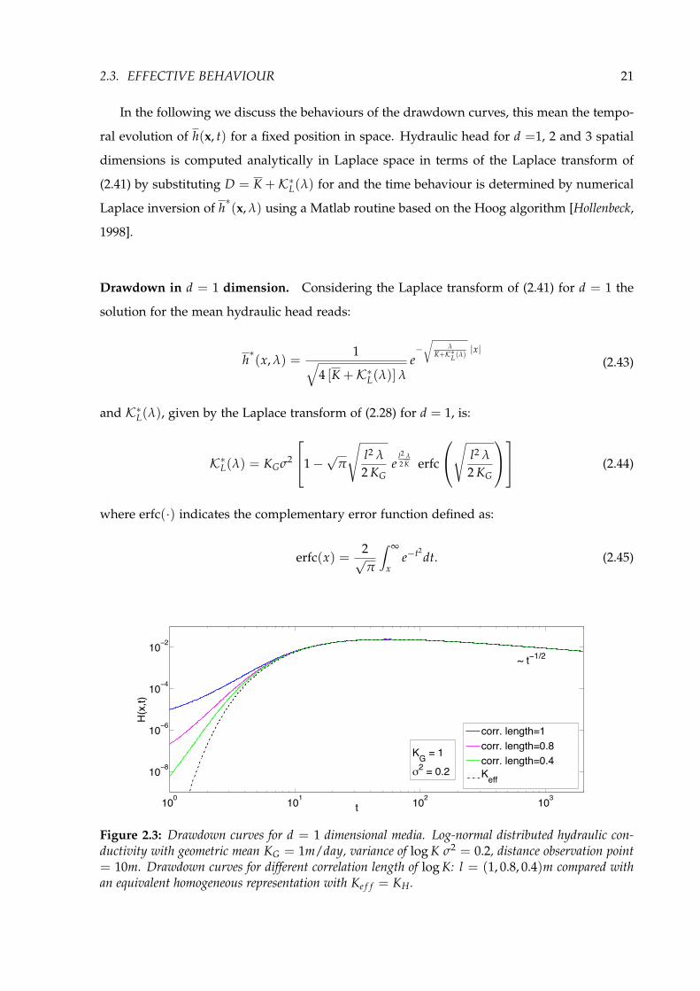
In the following we discuss the behaviours of the drawdown curves, this mean the tempo-
ral evolution of h(x, t) for a fixed position in space. Hydraulic head for d =1, 2 and 3 spatial
dimensions is computed analytically in Laplace space in terms of the Laplace transform of
(2.41) by substituting D = K + K∗L(λ) for and the time behaviour is determined by numerical
Laplace inversion of h∗(x, λ) using a Matlab routine based on the Hoog algorithm [Hollenbeck,
1998].
Drawdown in d = 1 dimension. Considering the Laplace transform of (2.41) for d = 1 the
solution for the mean hydraulic head reads:
h∗(x, λ) =1
4 [K + K∗L(λ)] λe−
λ
K+K∗L(λ) |x|(2.43)
and K∗L(λ), given by the Laplace transform of (2.28) for d = 1, is:
K∗L(λ) = KGσ2
1−√
π
l2 λ
2 KGe
l2 λ2 K erfc
l2 λ
2 KG
(2.44)
where erfc(·) indicates the complementary error function defined as:
erfc(x) =2√π
∞
xe−t2
dt. (2.45)
100 101 102 103
10 8
10 6
10 4
10 2
t
H(x
,t)
corr. length=1corr. length=0.8corr. length=0.4Keff
~ t 1/2
KG = 1 2 = 0.2
Figure 2.3: Drawdown curves for d = 1 dimensional media. Log-normal distributed hydraulic con-ductivity with geometric mean KG = 1m/day, variance of log K σ2 = 0.2, distance observation point= 10m. Drawdown curves for different correlation length of log K: l = (1, 0.8, 0.4)m compared withan equivalent homogeneous representation with Ke f f = KH.

22 CHAPTER 2. AVERAGED FLOW EQUATION
Figure 2.3 shows drawdown curves in d = 1 dimension for variable correlation lengths of
l = 0.4m, l = 0.8m and l = 1m. We display the solution of the non-local equation (solid lines)
and the local asymptotic equation (dash line). We observe that asymptotically drawdown
curves scale as t−1/2 as in the homogeneous case, but the drawdowns obtained for the non-
local equation arrives earlier than the equivalent homogeneous one. This behaviour can be
explained by the fact that the evolution of h(x, t) in the non-local case is influenced by the
values of conductivity at small times. In average conductivity at small time is given by the
arithmetic mean KA which is larger than the value of the asymptotic effective conductivity:
KA Ke f f . We furthermore observe that the drawdown curves arrive earlier with increasing
correlation length. For increasing l the length over which the pressure pulse is exposed to an
approximately constant local K value increases. Thus, in average, at small time the pressure
pulse is exposed to an equivalent conductivity higher than its asymptotic value for a large
time. This is also expressed by the evaluation of Ke(t) shows in figure 2.2. As shown in
Figure 2.2 the evolution of Ke(t) is governed by the characteristic time scale τK = l2/KG. For
increasing l, τK increases and Ke(t) is, at the same time larger than for a smaller correlation
length. This explains the earlier arrivals of drawdown for large correlation length.
1 102 4 810 10
10 8
10 6
10 4
10 2
t
H(x
,t)
2 = 0.2Keff, 2 = 0.2
2=0.1Keff, 2= 0.1
2= 0.3Keff, 2=0.3
KG = 1 corr. length = 0.6
Figure 2.4: Drawdown curves for 1 dimensional media. Log-normal distributed hydraulic conductivitywith geometric mean KG = 1m/day, correlation length of log K: l = 0.5m, distance observationpoint = 10m. Drawdown curves for different variance of log K: σ2 = 0.1, 0.2, 0.3 compared with anequivalent homogeneous representation with Ke f f = KH.
In Figure 2.4 we display drawdown curves for the non-local (solid) and the local asymptotic
(dash) models for variable log-conductivity variance. We observe that for the non-local model,
the drawdown arrive earlier with increasing heterogeneity, while for the effective asymptotic
formulation, the opposite holds. As noticed above, the non-local model is influenced by the
2.3. EFFECTIVE BEHAVIOUR 23
average conductivity at early times, which is larger that its asymptotic value. The arithmetic
mean KA = eσ2/2 increases with σ2 and consequently we have earlier arrival times. The local
asymptotic model is dominated by the harmonic mean KH = e−σ2/2, which decreases with
increasing σ2.
Drawdown in d = 2 dimension Considering d = 2 dimensional media, the hydraulic head
given by Laplace transform of (2.41), is:
h∗(x, λ) =1
2 π [ K + K∗L(λ)]K0
x2λ
K + K∗L(λ)
(2.46)
where K0(·) indicates the modified Bessel function of second kind of order zero and the kernel
K∗L(λ), from Laplace transform of (2.28) for d = 2, is:
K∗L(λ) = −KGσ2
2
1− l2λ
2KGe
l2λ2KG Ei
l2λ
2KG
(2.47)
where Ei(·) indicates the exponential integral function defined as:
Ei(x) = ∞
x
e−t
tdt, x > 0. (2.48)
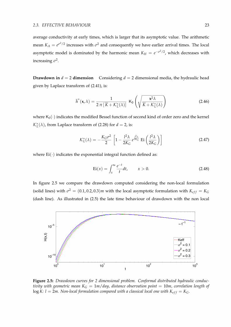
In figure 2.5 we compare the drawdown computed considering the non-local formulation
(solid lines) with σ2 = (0.1, 0.2, 0.3)m with the local asymptotic formulation with Ke f f = KG
(dash line). As illustrated in (2.5) the late time behaviour of drawdown with the non local
100 101 102 103
10 10
10 5
t
H(x
,t)
Keff2 = 0.12 = 0.22 = 0.3
~ t 1
Figure 2.5: Drawdown curves for 2 dimensional problem. Conformal distributed hydraulic conduc-tivity with geometric mean KG = 1m/day, distance observation point = 10m, correlation length oflog K: l = 2m. Non-local formulation compared with a classical local one with Ke f f = KG.
24 CHAPTER 2. AVERAGED FLOW EQUATION
formulation scales in time as t−1 as for the homogeneous case and for small variance the
non-local formulation tends to the homogeneous one, but, increasing the variance we get
earlier arrival times as in the d = 1 dimensional case. Notice that for d = 2 dimensional case,
differently that from d = 1, the effective conductivity Ke f f does not depend on the variance.
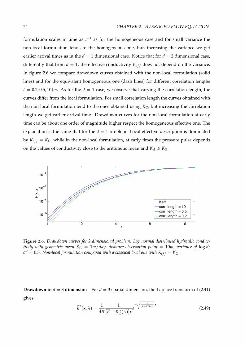
In figure 2.6 we compare drawdown curves obtained with the non-local formulation (solid
lines) and for the equivalent homogeneous one (dash lines) for different correlation lengths
l = 0.2, 0.5, 10)m. As for the d = 1 case, we observe that varying the correlation length, the
curves differ from the local formulation. For small correlation length the curves obtained with
the non local formulation tend to the ones obtained using KG, but increasing the correlation
length we get earlier arrival time. Drawdown curves for the non-local formulation at early
time can be about one order of magnitude higher respect the homogeneous effective one. The
explanation is the same that for the d = 1 problem. Local effective description is dominated
by Ke f f = KG, while in the non-local formulation, at early times the pressure pulse depends
on the values of conductivity close to the arithmetic mean and KA KG.
1 4 162 8
10 10
10 8
10 6
10 4
t
H(x
,t)
Keffcorr. length = 10corr. length = 0.5corr. length = 0.2
Figure 2.6: Drawdown curves for 2 dimensional problem. Log normal distributed hydraulic conduc-tivity with geometric mean KG = 1m/day, distance observation point = 10m, variance of log K:σ2 = 0.3. Non-local formulation compared with a classical local one with Ke f f = KG.
Drawdown in d = 3 dimension For d = 3 spatial dimension, the Laplace transform of (2.41)
gives:
h∗(x, λ) =1
4π
1[K + K∗L(λ)]x
e−
λ
[K+K∗L(λ)] x(2.49)
2.3. EFFECTIVE BEHAVIOUR 25
with the kernel K∗L(λ) given by:
K∗L(λ) = −KGσ2 13
1− 2l2λ
2KG+ 2√
π
l2λ
2KG
32
el2λ2K erfc
l2λ
2KG
. (2.50)
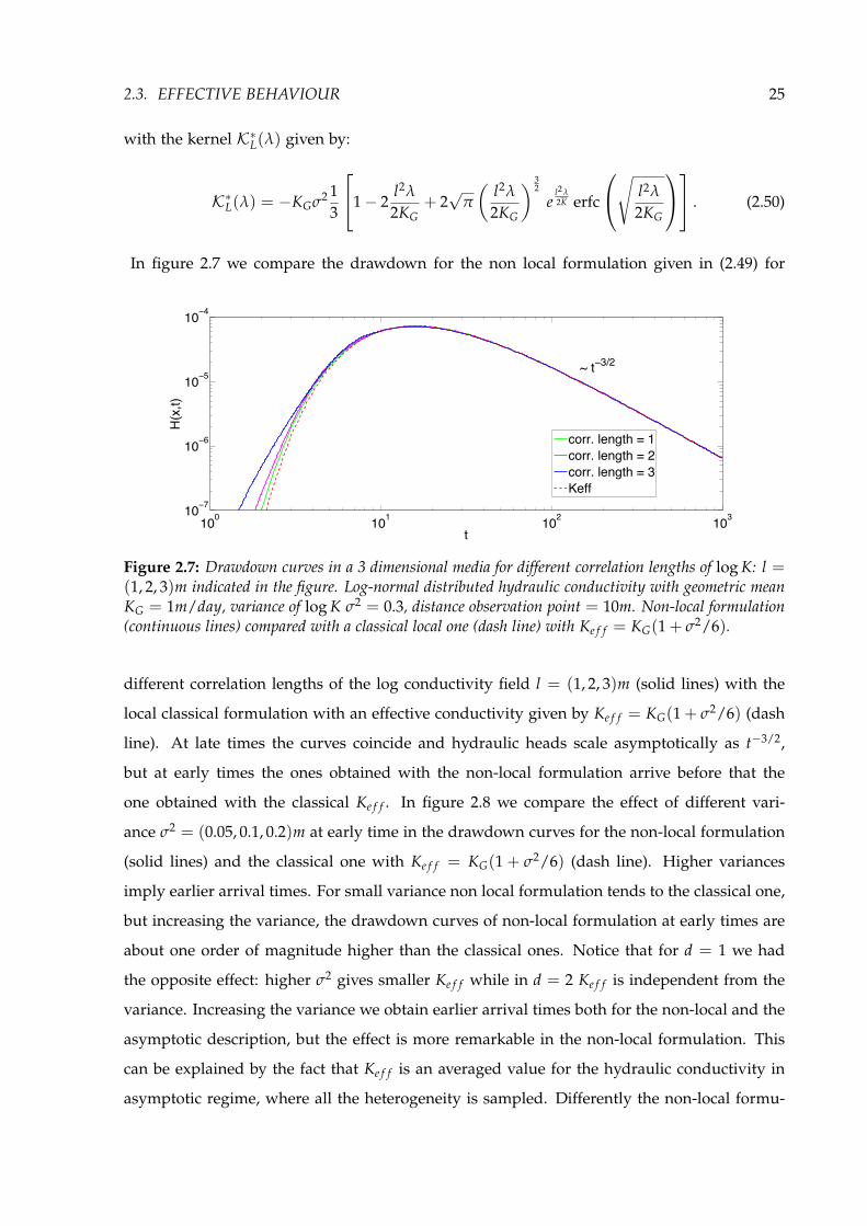
In figure 2.7 we compare the drawdown for the non local formulation given in (2.49) for
100 101 102 10310 7
10 6
10 5
10 4
t
H(x
,t)
corr. length = 1corr. length = 2corr. length = 3Keff
~ t 3/2
Figure 2.7: Drawdown curves in a 3 dimensional media for different correlation lengths of log K: l =(1, 2, 3)m indicated in the figure. Log-normal distributed hydraulic conductivity with geometric meanKG = 1m/day, variance of log K σ2 = 0.3, distance observation point = 10m. Non-local formulation(continuous lines) compared with a classical local one (dash line) with Ke f f = KG(1 + σ2/6).
different correlation lengths of the log conductivity field l = (1, 2, 3)m (solid lines) with the
local classical formulation with an effective conductivity given by Ke f f = KG(1 + σ2/6) (dash
line). At late times the curves coincide and hydraulic heads scale asymptotically as t−3/2,
but at early times the ones obtained with the non-local formulation arrive before that the
one obtained with the classical Ke f f . In figure 2.8 we compare the effect of different vari-
ance σ2 = (0.05, 0.1, 0.2)m at early time in the drawdown curves for the non-local formulation
(solid lines) and the classical one with Ke f f = KG(1 + σ2/6) (dash line). Higher variances
imply earlier arrival times. For small variance non local formulation tends to the classical one,
but increasing the variance, the drawdown curves of non-local formulation at early times are
about one order of magnitude higher than the classical ones. Notice that for d = 1 we had
the opposite effect: higher σ2 gives smaller Ke f f while in d = 2 Ke f f is independent from the
variance. Increasing the variance we obtain earlier arrival times both for the non-local and the
asymptotic description, but the effect is more remarkable in the non-local formulation. This
can be explained by the fact that Ke f f is an averaged value for the hydraulic conductivity in
asymptotic regime, where all the heterogeneity is sampled. Differently the non-local formu-

26 CHAPTER 2. AVERAGED FLOW EQUATION
1 82 410 9
10 8
10 7
10 6
10 5
10 4
t
H(x
,t)
2=0.1Keff 2=0.1
2=0.2Keff 2=0.2
2=0.05Keff 2=0.05
Figure 2.8: Drawdown curves in a 3 dimensional media for early times. Log-normal distributedhydraulic conductivity with geometric mean KG = 1m/day, variance of log K σ2 = 0.05, 0.1, 0.2,distance observation point= 20m, correlation length of log K: l = 3m. Non-local formulation comparedwith a classical local one with Ke f f = KG(1 + σ2/6).
lation takes into account the possibility that the pressure pulse reaches the observation point
without sampling all the heterogeneity, but ’choosing’ only the higher conductivity regions.
2.4 Conclusions
In this chapter we used a stochastic method to upscale flow in heterogeneous media charac-
terized by a spatially varying hydraulic conductivity and a constant storativity. In a stochastic
framework we modeled spatially varying hydraulic conductivity as multi-lognormal random
field and we derived an effective equation for the ensemble mean value of the hydraulic head.
The effective equation derived is non local. Non-locality is expressed by the convolution of
the gradient of the mean hydraulic head with a kernel that takes into account a statistical de-
scription of the heterogeneity of the conductivity field. Heterogeneity brings non-locality both
in time and in space in the flow problem an it implies that a description in terms of effective
coefficient is not enough to fully characterize flow in heterogeneous media. We demonstrate
the the well known values for the effective conductivity in d = 1, 2 and 3 dimensional media
can be obtained by localization of the effective equation derived. Localizing both in space and
in space the non local formulation derive we obtain a time dependent effective coefficient and
its asymptotic limit for d = 1, 2 and 3 spatial dimension reduces into the well known value for
effective conductivity in heterogeneous media. We show that effective conductivity computed
in terms of spatial moments for a pulse injection in an infinitive medium is equivalent to the
effective conductivity classically defined for a constant head gradient in a bounded domain.

2.4. CONCLUSIONS 27
Considering localization in space of the effective equation derived, we solved the non-local in
time formulation in Laplace space and we discussed the hydraulic response for a pulse injec-
tion in a d = 1, 2 and 3 spatial dimension. We compared the drawdown curves obtained with
the non-local formulation and with the classical local formulation and the well known values
for the effective conductivity Ke f f in d dimensions [Sanchez-Villa et al., 2006]. Asymptotically
the non-local formulation and the classical description coincide, but in the transient regime
the classical description underestimates earlier arrival times. Indeed the effective values of
Ke f f is defined for steady state condition, when all the heterogeneity is sampled. Non-local
formulation gives earlier arrival times and the effect increases as the variance and the corre-
lation length of the hydraulic conductivity field increase. Higher correlation length implies
longer transitional regime, which, in turns, implies higher underestimation of the earlier ar-
rival times using a local model. Correct estimation of early arrival times is highly important
in particular in groundwater vulnerability problem. The effect of underestimation of early
arrival times is less remarkable for increasing spatial dimension. This is due to the fact that
efficiency in the sampling of heterogeneity depends on the dimensionality of the problem:
increasing spatial dimension, heterogeneity is sampled with increasing efficiency and there-
fore steady state condition is reached earlier. It implies that increasing the dimensionality
of the problem the local description with Ke f f became earlier an effective description of the
heterogeneous problem. The efficiency in the sampling of the heterogeneity can be quantified
in a particle tracking framework, as we discuss in the following chapter dedicated to particle
tracking method. Considering a random walk, the efficiency in the sampling of heterogeneity
is given by the probability for a random walker to explore new sites, which increases with
increasing spatial dimension [Weiss, 1994]. This is reflected also on the temporal evolution
of the effective time dependent hydraulic conductivity Ke(t) computed by localization of the
kernel of the non-local equation in function of the spatial dimension d. Ke(t) tends to the well
known values of the hydraulic conductivity for any d dimension as t−1/2 for d = 1, as t−1 in
d = 2 and according to t−3/2 in d = 3.
28 CHAPTER 2. AVERAGED FLOW EQUATION

Chapter 3
Diffusion in Heterogeneous Media: a
Random Walk Perspective
I
3.1 Introduction
In this chapter we study diffusion in heterogeneous media characterized by spatially varying
diffusion properties using random walk. Diffusion in heterogeneous media is a ubiquitous
process in nature that describes a range of different physical phenomena [Haus and Kehr, 1987;
Havlin and Ben-Avraham, 2002b; Dean et al., 2007] including chemical transport in low perme-
ability media such as clays and granites [Delay et al., 2002] and in general in immobile regions
of a heterogeneous porous medium [Gouze et al., 2008b], Darcian fluid flow through heteroge-
neous media, heat transport and electric current through a conductor [King, 1987; Drummond
and Hogan, 1987; McCarthy, 1993], as well as diffusion in biological systems [Codling et al.,
2008]. The present work is motivated through the diffusion of chemicals in heterogeneous
low permeability media that are characterized by spatially varying diffusion properties. The
concentration c(x, t) of a dissolved chemical satisfies the diffusion equation
R(x)∂c(x, t)
∂t= ∇ · [D(x)∇c(x, t)] , (3.1)
IThe first part of this chapter has been published in the paper Diffusion and Trapping in Heterogeneous Media:An Inhomogeneous Continuous Time Random Walk Approach, Dentz M., P. Gouze, A. Russian, J. Dweik, F. Delay;Advances in Water Resources Advances in Water Resources 49 (2012) 13-22.
29

30CHAPTER 3. DIFFUSION IN HETEROGENEOUS MEDIA: A RANDOM WALK PERSPECTIVE
in which D(x) the diffusion coefficient and R(x) is a random retardation coefficient. Notice
that for diffusion of a non-reactive solute R(x) = φ(x) with φ(x) porosity. For diffusion under
linear equilibrium sorption-desorption reaction: R(x) = [1− φ(x)]kd(x) + φ(x) where kd is
the distribution coefficient that relates the mobile and the adsorbed concentration. For the case
of the flow of an incompressible fluid through a porous medium, c(x, t) represents hydraulic
head, R(x) = S(x) is the specific storativity and D(x)the hydraulic conductivity. The diffusion
equation (3.1) for heterogeneous media does not have a general closed form solution and is
often approached analytically using perturbation methods [Drummond and Hogan, 1987; King,
1987; Dean et al., 2007], and numerically using finite difference, finite element or finite volume
methods [Patankar, 1980; Crank, 1975]. In this paper, we focus on numerical approaches based
on random walk particle tracking [Kinzelbach, 1987; Drummond and Hogan, 1987]. This numeri-
cal method is based on the fact that equation (3.1) is equivalent to the Langevin equation [e.g.,
Gouze et al., 2008b]
dx(t)dt
=∇D[x(t)]
R[x(t)]+
2D[x(t)]R[x(t)]
ξ(t), (3.2)
in which x(t) describes the trajectories of the ’solute’ particles that constitute the concentration
distribution c(x, t). In fact, c(x, t) is expressed in terms of the particle trajectory as [Risken,
1996]
c(x, t) =1
R(x)δ[x− x(t)] , (3.3)
in which δ(x) denotes the d-dimensional Dirac delta-distribution.
The numerical solution of the Langevin equation (3.2) can be very costly because the het-
erogeneous diffusion properties may require a fine time-discretization in order to ensure that
a particle actually ’sees’ the spatial variability [e.g., James and Chrysikolpoulos, 2001; Delay et al.,
2002]. There may be inaccuracies because in some regions of the medium with little variability
a coarse discretization is sufficient while in regions with high variability a fine time discretiza-
tion is required [James and Chrysikolpoulos, 2001]. Also, as pointed out by McCarthy [McCarthy,
1993] in regions of small diffusivity a particle may have to wait at a given site for a large
number of simulation steps, which is inefficient. Furthermore, for pixelized maps of hetero-
geneous media as obtained by X-ray micro-tomography (XMT) [Delay et al., 2002; Gouze et al.,
2008b], see Figure 3.1, diffusion properties are spatially discontinuous, which makes the use

3.1. INTRODUCTION 31
of Eq. (3.2) complicated because it relies on the calculation of the gradient of the diffusion
coefficient D(x) (see for example [Delay et al., 2005]). Therefore, there is a need for random
walk scheme that can handle this kind of problems. The time domain random walk (TDRW)
approach represents an alternative to the classical random walk (RW) framework. In Section
4.2 we present a rigorous derivation of the TDRW algorithm and a demonstration its equiva-
lence to the diffusion equation. Furthermore, we extend the TDRW to solve diffusion problem
in a heterogeneous medium with multi-rate mass transfer properties using a statistical repre-
sentation of the medium.
Figure 3.1: Left: Numerical cross-section of a connected pore cluster obtained from a d = 3 dimensionalXMT image (5 mm × 5 mm limestone sample), the black color indicates pore space. Right: Equivalentupscaled porosity map. The arrows indicate possible particle transitions to nearest neighbors.
Heterogeneity brings complexity in diffusion problems, which, in turn, induces uncer-
tainty and anomalous behaviour [Havlin and Ben-Avraham, 2002b; Bouchaud and Georges, 1990].
There are many model that describe non-Fickian/anomalous diffusion phenomena, like CTRW
[Berkowitz et al., 2006; Metzler and Klafter, 2000], delayed-diffusion models [Dentz and Tar-
takovsky, 2006], MRMT models [Haggerty and Gorelick, 1995; Carrera et al., 1998] fractional
diffusion models [Metzler and Klafter, 2000]. Oftentimes these approaches are not linked to
the heterogeneity distribution, which puts a limitation on their predictive capability. Stochas-

32CHAPTER 3. DIFFUSION IN HETEROGENEOUS MEDIA: A RANDOM WALK PERSPECTIVE
tic modeling provides a systematic way to quantify the heterogeneity impact on diffusion in
heterogeneous media, see also Chapter 3. In section 4.3 we discuss the upscaling of diffusion
in a d = 3 spatial dimension medium characterized by varying R(x) and constant D(x) = D.
Using a stochastic modeling approach we derive an explicit non-local diffusion equation for
the average particle density.
3.2 Time Domain Random Walk
As pointed out in the introduction, numerical solution of Langevin equation can be very
costly, here we present a particle scheme that relies on spatial increments, whose absolute val-
ues are deterministic, combined with random time increment [McCarthy, 1993; Banton et al.,
1997; Noetinger and Estebenet, 2000; James and Chrysikolpoulos, 2001; Delay et al., 2002; Reimus
and James, 2002]. That is, at each random walk step the particle moves a given distance (which
can be given by the pixel size of the discretized medium representation, for example) in a ran-
dom direction, whose probability is calculated from the diffusion properties of the medium.
The time for the step is random, which reflects the stochastic nature of the diffusion process.
There has been in fact a certain ambiguity on how to model the distribution of transition
time. In [McCarthy, 1993], Noetinger and Estebenet [2000] and Delay et al. [2002], for example,
an exponential transition time distribution is employed, while James and Chrysikolpoulos [2001]
and Delay and Bodin [2001] use a log-normal transition time distribution. Ref. [Reimus and
James, 2002] identifies the transition time with the first-passage time to cross a certain distance
by diffusion. The different variants of this methodology have been called continuous time
random walk (CTRW) on random media [McCarthy, 1993; Noetinger and Estebenet, 2000] and
time-domain random walk (TDRW) [Banton et al., 1997; James and Chrysikolpoulos, 2001]. In the
different aforementioned applications, TDRW method has been used for the determination
of effective diffusivity [Delay et al., 2002], effective hydraulic and electrical conductivity [Mc-
Carthy, 1993], for the upscaling of fluid flow in fractured rocks [Noetinger and Estebenet, 2000]
and for the efficient simulation of chemical transport in fracture networks [Delay and Bodin,
2001; Bodin et al., 2003].
The TDRW method is closely related to the continuous time random walk (CTRW) frame-
work [Montroll and Weiss, 1965; Scher and Lax, 1973]. A CTRW describes the stochastic move-
ment of particles as random walk in space and time. The CTRW approach has been used
for the modeling of electron transport in disordered media Scher and Lax [1973], diffusion in

3.2. TIME DOMAIN RANDOM WALK 33
turbulence [Zumofen and Klafter, 1993], chemical transport in heterogeneous porous media, to
name but a few, see also the exhaustive review paper by Berkowitz et al. Berkowitz et al. [2006].
It has been used successfully to model anomalous transport features in fluctuating environ-
ments. In this context it can be seen as an average transport framework that is based on the
observation that, when looking at average Lagrangian transport dynamics, particles may need
different times to cross the same distance, due to heterogeneous medium properties. Effective
particle dynamics can be described as a CTRW. This is the reason why CTRW is often referred
to as an ensemble averaged transport model. Strictly speaking, it is a model that describes
particle movements as a random walk in space and time coordinates. As pointed out above,
McCarthy [McCarthy, 1993] and Noetinger and Estebenet [Noetinger and Estebenet, 2000] refer
to TDRW as a CTRW method because the time increment is random. The papers on TDRW,
we reviewed above, propose a TDRW algorithm as an efficient solution methodology for the
heterogeneous diffusion equation. However, in none of these papers, have we found a demon-
stration of the formal equivalence of the TDRW algorithm and the diffusion equation, as it
exists for the equivalence of the diffusion equation (3.1) and the Langevin equation (3.2).
3.2.1 Theoretical Development
The solution of the diffusion equation in a classical RW scheme based on equation (3.2) can
be very costly. In this section we present an efficient particle tracking scheme to solve flow in
heterogeneous media.
In this section, we first consider a continuous time random walk (CTRW) [Montroll and
Weiss, 1965; Scher and Lax, 1973; Berkowitz et al., 2006] on an inhomogeneous spatial lattice,
which is characterized by non-stationary spatial transition probabilities and space-dependent
transition time distribution [Berkowitz et al., 2002; Goychuk, 2004; Chechkin et al., 2005]. We then
show that the inhomogeneous CTRW with an exponential transition time distribution solves
the discrete equations that describe diffusion in heterogeneous media. This demonstrates the
equivalence of the time-domain random walk (TDRW) scheme, which was developed for the
solution of heterogeneous diffusion problems [McCarthy, 1993; Noetinger and Estebenet, 2000;
Delay et al., 2002], and CTRW. Based on these results, we discuss an extension of the TDRW
method for heterogeneous diffusion in combination with heterogeneous trapping properties.

34CHAPTER 3. DIFFUSION IN HETEROGENEOUS MEDIA: A RANDOM WALK PERSPECTIVE
3.2.1.1 Spatially Inhomogeneous CTRW
We consider a spatially inhomogeneous continuous time random walk (CTRW) [e.g., Montroll
and Weiss, 1965; Scher and Lax, 1973] on a lattice defined by the following set of recursion
equations
xi(n + 1) = xj(n) + ξ ij, tn+1 = tn + θj, (3.4)
where the position of lattice point j is denoted by xj. The probability for a spatial transition
ξij between points j and i (i.e. from j to i) is given by wij, the probability density of the
random time increment θj depends on the position of the particle at step n. Its distribution is
given by the transition time density ψj(t). Equation (3.4) describes an inhomogeneous CTRW
because the probabilities wij and ψj(t) for spatial and temporal particle transitions depend on
the particle positions within the lattice.
The particle density gi(t) at point i is defined by
gi(t) =∆[xi − xj(t)]
. (3.5)
The angular brackets denote the average over all particles that are launched in the random
walk (3.4) and the function ∆[xi − xj(t)] is 1 if xj(t) = xi and zero otherwise. The random
walk (3.4) describes time as a stochastic process. The number of steps needed to reach time t
is counted by the renewal process nt = max(n|tn ≤ t). The number density gi(t) then reads
in terms of the space-time particle trajectories (3.4) as
gi(t) =∆[xi − xj(nt)]
. (3.6)
This expression can be expanded as
gi(t) =∞
∑n=0
∆[xi − xj(n)]δn,nt
. (3.7)
The statement n = nt is equivalent to 0 ≤ t− tn < θi. This condition can be expressed by the
product of two Heaviside functions H(·). Thus, we can write gi(t) as
gi(t) =∞
∑n=0
∆[xi − xj(n)] H[(θi − (t− t)] H(t− t)
. (3.8)

3.2. TIME DOMAIN RANDOM WALK 35
By inserting a Dirac-delta, we obtain
gi(t) =∞
∑n=0
t
0dt
∆[xi − xj(n)]δ(t − tn)
H(θj − (t− t)
. (3.9)
We could break the noise average because of the Markovianity of the process (3.4). Executing
the second average explicitly and defining Ri(t) = ∑∞n=0
∆[xi − xj(n)]δ(t− tn)
, we obtain
gi(t) =t
0
dtAi(t)∞
t−t
dτψi(τ). (3.10)
The Ai(t) describes the probability per time for the particle to just arrive at xi at time t. From
the Markovianity of the process (3.4) we obtain for Ri(t) that
Ai(t) = ρiδ(t) + ∑[ik]
wik
t
0
dtψk(t− t)Ak(t), (3.11)
with ρi = gi(t = 0) the initial particle density at point xi. Notice that (3.11) is a Chapman-
Kolmogorov type equation that describes the probability to just arrive at xi at time t as the
sum over all possible transitions from a position xk to xi of duration t− t. The notation ∑[ik]
indicates summation over nearest neighbors of pixel i. Combination of (5.32) and (3.11) in
Laplace space gives for the Laplace transform of gi(t) the well known generalized Master
equation [e.g., Kenkre et al., 1973]
λg∗i (λ) = ρi + ∑[ik]
wikλψ∗k (λ)1− ψ∗k (λ)
g∗k (λ)− λψ∗i (λ)1− ψ∗i (λ)
g∗i (λ). (3.12)
The Laplace transform is defined in Abramowitz and Stegun [1965]. Here and in the following,
Laplace transformed quantities are marked by an asterisk, the Laplace variable is denoted by
λ.
3.2.1.2 Equivalence with Heterogeneous Diffusion
In order to establish the equivalence between the inhomogeneous CTRW detailed in in the
previous section and the heterogeneous diffusion equation (3.1), we consider the exponential
transition time density [Berkowitz et al., 2006]
ψj(t) = τ−1j exp(−t/τj). (3.13)

36CHAPTER 3. DIFFUSION IN HETEROGENEOUS MEDIA: A RANDOM WALK PERSPECTIVE
Inserting the Laplace transform of (4.7) into (3.12) gives
λg∗i (λ) = ρi + ∑[ij]
wijτ−1j g∗k (λ)− τ−1
i g∗i (λ). (3.14)
Transforming this equation back to real time, we obtain the Master equation
∂gi∂t
= ∑[ij]
wijτ−1j gj − τ−1
i gi. (3.15)
We now define the transition probabilities wij and transition times τj as
wij =bij
∑[jk] bkj, τj =
1∑[kj] bkj
, (3.16)
where the bij are defined below. By definition the wij fulfill the normalization condition
∑[ji] wij = 1. Inserting these definitions into (3.15), we obtain
∂gi∂t
= ∑[ij]
bijgj −∑[ki]
bkigi. (3.17)
Notice that for bij = bji, this equation describes diffusion on a lattice with symmetric barri-
ers [e.g., Bouchaud and Georges, 1990].
To establish the equivalence of the Master equation (3.17) and the diffusion equation (3.1),
we need to further specify the bij in terms of the retardation coefficient and diffusion coeffi-
cients. Thus, we define now
bij =bij
VjRj, bij =
SijDij
ξij, (3.18)
where Vj and Rj are volume and retardation coefficient of pixel j, respectively, Sij denotes the
surface area between pixels i and j and Dij is an average diffusion coefficient between pixels i
and j, see Section 3.2.2.1. Notice that the bij are symmetric by definition, while the bij and thus
the transition probabilities wij are in general not. Furthermore, we define the rescaled particle
density
ci =gi
ViRi. (3.19)

3.2. TIME DOMAIN RANDOM WALK 37
Inserting (5.14) and (3.19) into (3.17) gives
ViRi∂ci∂t
= ∑[ij]
bijcj −∑[ij]
bijci. (3.20)
This equation together with definition (5.14) of the bij corresponds to a finite volume dis-
cretization of (3.1) as outlined for example in Delay et al. [2002]. The quantity ci is identified
with the solute concentration in the fluid phase. Thus, in the limit ξij → 0, we obtain the
heterogeneous diffusion equation (3.1). This establishes the equivalence between (3.1) and the
CTRW scheme (3.4) for the transition probabilities wij and mean transition times τj defined as
wij =bij
∑[jk] bkj, τj =
VjRj
∑[kj] bkj, (3.21)
where we used (5.14) in (3.16). Notice that the random walk algorithm based on (3.4) and (3.16)
for the exponential ψi(t) (4.7) is identical to the time domain random walk (TDRW) presented
by Delay et al. [2002]. Delay et al. Delay et al. [2002] deduced the exponential transition time
distribution (4.7) by interpreting (3.20) in terms of single particle transitions. This explicit
demonstration, removes ambiguity with respect to the distribution of transition times.
3.2.1.3 Heterogeneous Diffusion With Multirate Mass Transfer (MRMT)
In the previous section we established the equivalence between the spatially discrete hetero-
geneous diffusion equation (3.1) and the inhomogeneous CTRW (3.4) with (4.7) and (3.21), or
in other words, a TDRW. Here we consider the generalization of this framework to heteroge-
neous diffusion combined with multirate mass transfer (MRMT). The MRMT approach [e.g.,
Haggerty and Gorelick, 1995; Carrera et al., 1998] describes transport in the presence of traps, or
immobile zones, in which the solute can be immobilized for a certain amount of time. The
trapping mechanisms may be chemical such as adsorption, or physical, such as very slow
diffusion. It has been shown in Refs. [Dentz and Berkowitz, 2003] and [Benson and Meerschaert,
2009] that the CTRW and multirate mass transfer modeling approaches are equivalent under
certain conditions. Thus, based on these results and on the observation that a TDRW describes
an inhomogeneous CTRW, we develop in the following a TDRW approach that models particle
transport in heterogeneous media under spatially varying diffusion and trapping properties.
As in the previous section, we start with the formulation of MRMT as an inhomogeneous
CTRW. We then consider the corresponding generalized Master equation and establish the

38CHAPTER 3. DIFFUSION IN HETEROGENEOUS MEDIA: A RANDOM WALK PERSPECTIVE
equivalence to the spatially heterogeneous diffusion equation with spatially variable mass
transfer. Linear multirate sorption-desorption and in general linear multirate mass trans-
fer can be modeled in the framework of CTRW by introducing a trapping time distribution
p(t) [e.g., Margolin et al., 2003]. The particle transition time then is given by the time spent
in the mobile domain and the sum of trapping times during a transition. The transition time
distribution ψ(t) with traps then is given in terms of the transition time distribution ψ0(t)
without traps as [Margolin et al., 2003]
ψ∗(λ) = ψ∗0 (λ + α [1− p∗(λ)]) , (3.22)
in which α is the trapping frequency during a transition. Benson and Meerschaert Benson and
Meerschaert [2009] studied the case for which the transition time without traps is exponentially
distributed using random walk particle tracking. A similar approach was used by Delay and
co-workers [Delay and Bodin, 2001; Delay et al., 2008] to extend the TDRW method to account
for matrix diffusion in the context of transport in fractured media.
Here, we consider the general case that the trapping time distribution pj(t) and trapping
frequency αj depend on position. Using the Laplace transform of the exponential distribu-
tion (4.7) for ψ∗0(t) in (3.22), we obtain for the ψj(t) of heterogeneous diffusion and MRMT the
expression
ψ∗j (λ) =1
1 + λτj + αjτj[1− p∗j (λ)]. (3.23)
Inserting this explicit form in the generalized Master equation (3.12) gives
λg∗i (λ) = ρi + ∑[ik]
wikλg∗k (λ)λτk + αkτk[1− p∗k (λ)]
− λg∗i (λ)λτi + αiτi[1− p∗i (λ)]
. (3.24)
In order to obtain the partial differential equation that governs transport under heterogeneous
MRMT, we identify the wik in (3.24) with
wik =bikτkVkRk
, (3.25)
where we used (3.16) and (5.14). Furthermore, we set gi = RiVici, see (3.19). Thus, we can
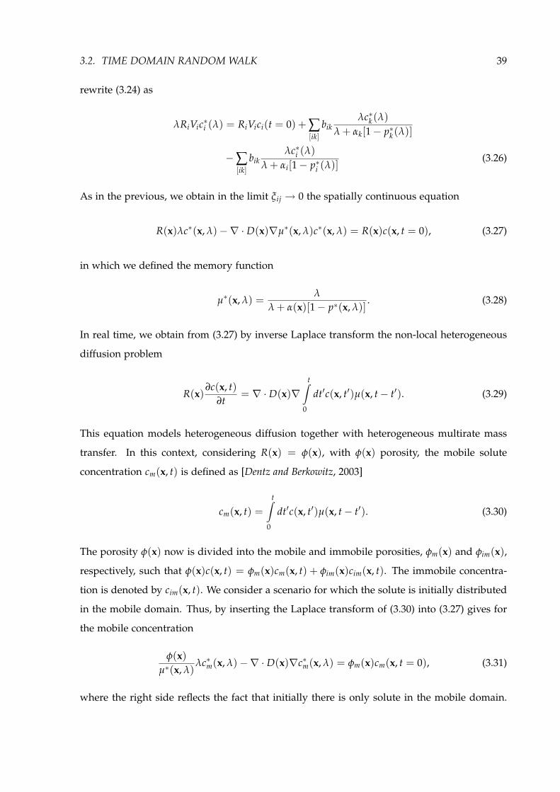
3.2. TIME DOMAIN RANDOM WALK 39
rewrite (3.24) as
λRiVic∗i (λ) = RiVici(t = 0) + ∑[ik]
bikλc∗k (λ)
λ + αk[1− p∗k (λ)]
−∑[ik]
bikλc∗i (λ)
λ + αi[1− p∗i (λ)](3.26)
As in the previous, we obtain in the limit ξij → 0 the spatially continuous equation
R(x)λc∗(x, λ)−∇ · D(x)∇µ∗(x, λ)c∗(x, λ) = R(x)c(x, t = 0), (3.27)
in which we defined the memory function
µ∗(x, λ) =λ
λ + α(x)[1− p∗(x, λ)]. (3.28)
In real time, we obtain from (3.27) by inverse Laplace transform the non-local heterogeneous
diffusion problem
R(x)∂c(x, t)
∂t= ∇ · D(x)∇
t
0
dtc(x, t)µ(x, t− t). (3.29)
This equation models heterogeneous diffusion together with heterogeneous multirate mass
transfer. In this context, considering R(x) = φ(x), with φ(x) porosity, the mobile solute
concentration cm(x, t) is defined as [Dentz and Berkowitz, 2003]
cm(x, t) =t
0
dtc(x, t)µ(x, t− t). (3.30)
The porosity φ(x) now is divided into the mobile and immobile porosities, φm(x) and φim(x),
respectively, such that φ(x)c(x, t) = φm(x)cm(x, t) + φim(x)cim(x, t). The immobile concentra-
tion is denoted by cim(x, t). We consider a scenario for which the solute is initially distributed
in the mobile domain. Thus, by inserting the Laplace transform of (3.30) into (3.27) gives for
the mobile concentration
φ(x)µ∗(x, λ)
λc∗m(x, λ)−∇ · D(x)∇c∗m(x, λ) = φm(x)cm(x, t = 0), (3.31)
where the right side reflects the fact that initially there is only solute in the mobile domain.

40CHAPTER 3. DIFFUSION IN HETEROGENEOUS MEDIA: A RANDOM WALK PERSPECTIVE
We now establish the relation between the memory function µ(x, t) and the transfer function
ϕ(x, t) given within the context of MRMT. The MRMT approach gives the following non-local
transport equation for the mobile concentration [e.g., Carrera et al., 1998; Haggerty et al., 2000]
φm(x)∂cm(x, t)
∂t+ φim(x)
∂
∂t
t
0
dtϕ(x, t− t)cm(x, t)
= ∇ · D(x)∇cm(x, t). (3.32)
The difference to the formulations given in Refs. Carrera et al. [1998]; Haggerty et al. [2000]
are due to the non-zero initial condition employed here. The site-dependent transfer function
ϕ(x, t) encodes the details of the microscopic mass transfer mechanisms between the mobile
and immobile regions [e.g., Harvey and Gorelick, 1995; Dentz and Berkowitz, 2003]. Comparing
the Laplace transform of (3.32) with (3.31) gives the following relation between the memory
function µ∗(x, λ) and the transfer function ϕ∗(x, λ)
µ∗(x, λ) =φ(x)
φm(x) + φim(x)ϕ∗(x, λ). (3.33)
For the relation between the Laplace transforms of the transfer function, ϕ∗(x, λ), and the
trapping time distribution, p∗(x, λ), we obtain by using (3.28)
ϕ∗(x, λ) =φ(x)
φim(x)− φm(x)
φim(x)+
α(x)φ(x)φim(x)λ
[1− p∗(x, λ)] . (3.34)
3.2.2 Model Setup and Numerical Implementation
We consider diffusion in the d-dimensional domain Ω with the (d− 1)-dimensional bound-
aries BΩ. In the following we use regular meshes in d = 2 and d = 1 spatial dimensions.
Consequently the internodal distance is ξij = ξ is constant. Thus, the interfacial area Sij be-
tween the pixels i and j is constant and given by S = ξd−1 and so is the volume of the pixel,
Vi = V = ξd. The normalized transition probability wij from position j to position i is given
by (5.14).
No flow boundary conditions are treated as a zero diffusion limit (wij = 0). Dirichlet
boundary conditions at the inlet BinΩ ⊂ BΩ (constant concentration) are implemented as de-
scribed in the following. The inlet BinΩ is formed by Pin pixels. At each of these pixels the
concentration is constant, ci = cin for i = 1, . . . , Pin. Note that for d = 1 spatial dimension
Pin = 1. In the numerical particle tracking simulations, however, we do not prescribe the

3.2. TIME DOMAIN RANDOM WALK 41
concentration at the inlet boundary, but the number of particles at each node. Therefore, we
consider the number density gi given by (3.19). Its values at the boundary nodes is given
by gini = RiVcin. Since the gi are in general not normalized, we define now the normalized
number density as
ni =gi
∑Pinj=1 gin
j
=Rici
cin ∑Pinj=1 Rj
. (3.35)
This is the observable that we obtain from the TDRW simulations, namely ni is equal to the
number Ni of particles in the pixel normalized by the number of particles N on the boundary,
ni = Ni/N. Thus, the concentration ci at pixel i is given in terms of the ni as
ci = nicin ∑Pin
j=1 Rj
Ri. (3.36)
The number Nini of particles at the boundary pixels then are given by
Nini = N
Ri
∑Pinj=1 Rj
(3.37)
for i = 1, . . . , Pin.
An absorbing boundary condition (zero concentration) at the outlet boundary BoutΩ ⊂ Ω is
implemented by removing particles as they cross BoutΩ . The outlet boundary is formed by Pout
pixels. Note that Pout = 1 in d = 1 spatial dimension. The cumulative distribution of arrival
times F(t) at the outlet boundary then is given by
F(t) =1N
Pout
∑j=1
Nj(t), (3.38)
where Nj(t) is the number of particles that have crossed the outlet boundary until time t.
Correspondingly, the distribution density of arrival times, f (t), is
f (t) =1N
Pout
∑j=1
∆Nj(t)∆t
, (3.39)
where ∆Nj(t) is the number of particles that crosses the outlet during the sampling interval
[t, t + ∆t].

42CHAPTER 3. DIFFUSION IN HETEROGENEOUS MEDIA: A RANDOM WALK PERSPECTIVE
3.2.2.1 Interpixel Diffusion Coefficients
In Section 3.2.1.2, we left intentionally open how to choose the interpixel diffusion coefficients
Dij. Frequently, it is determined as the harmonic average between the diffusion coefficient in
adjacent pixels [e.g., Delay et al., 2002]. Here we want to compare the performance of different
choices for the interpixel diffusion coefficient.
To this end, we consider diffusion in a two-dimensional domain of length L = 102ξ and
width d = 50ξ. It is characterized by a spatially varying diffusion coefficient D(x) and constant
retardation R(x) = R = 1. The heterogeneous domain is generated by assigning to each
pixel in the domain randomly diffusion coefficients that are chosen independently, from a
lognormal distribution characterized by the geometric average DG = 0.5 and variance of ln D
given by σ2ln D = 1. We record the vertically averaged concentration close to the outlet at
x1 = 90ξ and compare it to the analytical solution for the equivalent homogeneous problem.
Specifically, we consider the case of an instantaneous solute pulse at the inlet boundary at
x1 = 0. The position vector here is x = (x1, x2)T.
It was shown by Matheron [1967] that the exact effective diffusion coefficient De for this
setup is given by the geometric mean De = DG of the lognormally distributed D(x). Thus, the
equivalent homogeneous diffusion problem for c(x1, t) = d−1 d0 dx2c(x, t) is one-dimensional
and characterized by the geometric mean diffusion coefficient DG,
∂c(x1, t)∂t
− DG∂2c(x1, t)
∂x21
= 0, (3.40)
with the initial condition c(x1, t = 0) = 0. The boundary condition at the outlet is c(L, t) = 0,
the one at the inlet is c(0, t) = j0δ(t). The solute flux j0 is given by j0 = c0τp with c0 the
concentration on the inlet boundary and τp the pulse duration. The analytical solution for
c(x1, t) then is given by [e.g., Carslaw and Jaeger, 1947]
c(x1, t) = j02DGπ
L2
∞
∑n=1
n sinnπx1
L
exp
−n2DGπ2t
L2
, (3.41)
In the following d = 2 dimensional numerical simulations, we apply the concentration
c0 = 1/ξ2. The pulse duration τp is given by the mean diffusion time over one pixel τp =
ξ2/(2DG). Thus, we have j0 = 1/(2DG). At the horizontal boundaries at x2 = 0 and x2 = d
no-flux boundary conditions are specified. The domain size is L = 10 m.
We compare this analytical solution for the exact average diffusion problem (3.40) to the

3.2. TIME DOMAIN RANDOM WALK 43
outcome of the corresponding TDRW simulations for two difference choices of the interpixel
diffusion coefficient, namely (i) the harmonic mean and (ii) the geometric mean of the diffu-
sion coefficients in adjacent pixels. The choice that yields the best comparison with the exact
average solution will be employed in the following numerical simulations.
0
0.5
1
1.5
2
2.5
3
3.5
0 20 40 60 80 100 120 140 160 180 200
c(x 1
, t) ×
103
t
Figure 3.2: Vertically averaged concentration at x = 9 m for diffusion in a heterogeneous mediumcharacterized by a log-normally distributed diffusion coefficient. Comparison of the numerical solutionsfor interpixel diffusion coefficients given by the (squares) harmonic and (triangles) geometric mean,and the (solid line) analytical solution (3.41) with DG = 0.52 m2s−1, and L = 10 m. The number ofpixels used in the TDRW simulation in horizontal direction is 102 and in vertical direction 50. Thesimulations were performed using N = 5× 10⁸ particles.
Figure 3.2 displays the vertically averaged and normalized concentration cL(t) close to
the outlet boundary at L = 90ξ obtained from the TDRW simulation for the two different
interpixel diffusion coefficients. It is compared to c(x1, t) for the equivalent homogeneous
medium given by (3.41) with DG = 0.52. We observe that the interpixel diffusion coefficient
given by the geometric mean gives the best agreement with the analytical solution. Therefore,
in the following d = 2 dimensional TDRW simulations we will employ the geometric mean
for the interpixel diffusion coefficients
Dij =
DiDj. (3.42)

44CHAPTER 3. DIFFUSION IN HETEROGENEOUS MEDIA: A RANDOM WALK PERSPECTIVE
Note that it is beyond the scope of the present paper to demonstrate that it is the best ap-
proximation for non-lognormal distributions or for three-dimensional transport. This issue
is in fact not specific to the TDRW approach but concerns all discretized methods applied to
heterogeneous diffusion problems.
For the d = 1 dimensional TDRW simulations presented in the following, the interpixel
diffusion coefficient is given by the harmonic mean
Dij = DH = 2DiDj
Di + Dj. (3.43)
The pulse duration τp is as above given by the mean diffusion time over one pixel τp =
ξ2/(2DH), the boundary concentration, however, is c0 = 1/ξ. Thus, for d = 1 we have
j0 = ξ/(2DH).
Also note that the setup considered here corresponds to a pulsed through diffusion test.
Diffusion experiments (or through diffusion tests) are widely used for measuring the effec-
tive diffusion of low permeability porous media, such as manufactured cements or consoli-
dated argillaceous formations considered as potential host rock for radioactive waste reposi-
tories [Wittebroodt et al., 2008]. At the laboratory scale such experiments consist in applying a
constant concentration gradient across a thin core of rock by maintaining constant concentra-
tion at the two edges (usually a zero concentration at the outlet) and recording the solute flux
at the outlet [Pabitra, 2004].
3.2.2.2 Heterogeneous Diffusion
The heterogeneous diffusion problem (3.1) is solved using the random walk particle tracking
scheme (3.4) with the transition time density (4.7) and the transition probabilities wij and
the mean transition time τj given by (3.21). The transport time is updated for each particle
transition according to
tn+1 = tn + θj, θj = −τj ln(ηn), (3.44)
where the random variable ηn is uniformly distributed in [0, 1].

3.2. TIME DOMAIN RANDOM WALK 45
3.2.2.3 Diffusion with Multirate Mass Transfer
In Section 3.2.1.3, we showed that MRMT can be modeled in the TDRW context by introducing
particle traps characterized by a given distribution of trapping times. The resulting TDRW-
MRMT model is implemented following Ref. [Benson and Meerschaert, 2009]. First, we note
that the transition time θj, which is distributed according to (4.7), measures the total time the
particle is mobile. During this mobile time, the particle can get trapped at the constant rate
αj, see Section 3.2.1.3. The times the particle are mobile between trapping events is denoted
by θj. Since trapping occurs at constant rate, θj is exponentially distributed
pmj(t) = αj exp(−αjt). (3.45)
The number of trapping events that actually occur during a mobile transition of time θj, nθj ,
is the random number that fulfills
nθj = max
n
n
∑l=1
θjl ≤ θj <n+1
∑l=1
θjl
. (3.46)
It is a renewal process, and specifically, for the exponential distribution (3.45), it is a Poisson
process. The distribution pn(n|θj) of nθj thus is given by the Poisson distribution
pn(n|θj) =(αjθj)n
n!exp(−αjθj). (3.47)
The unconditional distribution of the number of trapping events at pixel j then is given by
pnj(n) =∞
0
dtψj(t)pn(n|t) =n(αjτj)n
(αjτj + 1)n+1 , (3.48)
in which we used (4.7) for ψj(t). Thus, the mean number of trapping events nj at pixel j is
given by nj = αjτj. The overbar in the following denotes the noise average over all particles.
The spatial average of the mean numbers of trapping events per pixel is Ntrap = nj. The
spatial average over all pixels is denoted by angular brackets.
In general, the trapping rate αj is spatially distributed and can be considered as a property
of the heterogeneous medium. For the following analysis, we correlate the trapping rate
to porosity φ(x) that we substitute instead of the generic retardation coefficient R(x) and
assume that the noise mean number of traps at pixel j is inversely proportional to porosity,
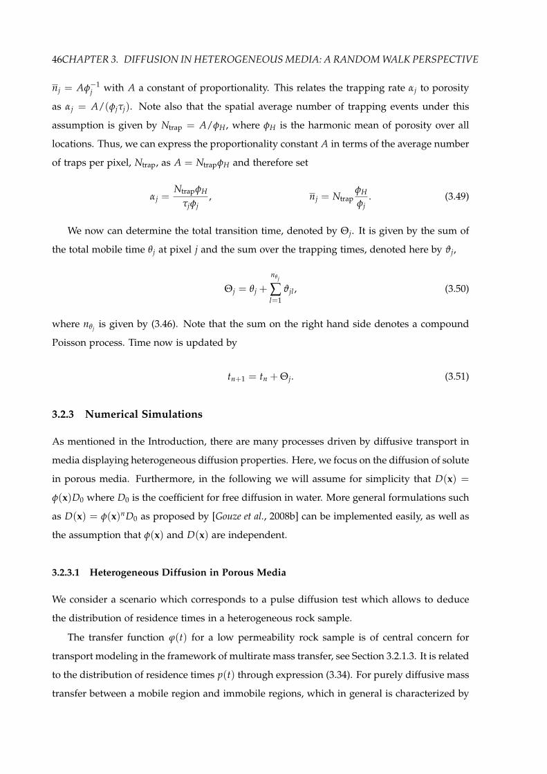
46CHAPTER 3. DIFFUSION IN HETEROGENEOUS MEDIA: A RANDOM WALK PERSPECTIVE
nj = Aφ−1j with A a constant of proportionality. This relates the trapping rate αj to porosity
as αj = A/(φjτj). Note also that the spatial average number of trapping events under this
assumption is given by Ntrap = A/φH, where φH is the harmonic mean of porosity over all
locations. Thus, we can express the proportionality constant A in terms of the average number
of traps per pixel, Ntrap, as A = NtrapφH and therefore set
αj =NtrapφH
τjφj, nj = Ntrap
φH
φj. (3.49)
We now can determine the total transition time, denoted by Θj. It is given by the sum of
the total mobile time θj at pixel j and the sum over the trapping times, denoted here by ϑj,
Θj = θj +nθj
∑l=1
ϑjl , (3.50)
where nθj is given by (3.46). Note that the sum on the right hand side denotes a compound
Poisson process. Time now is updated by
tn+1 = tn + Θj. (3.51)
3.2.3 Numerical Simulations
As mentioned in the Introduction, there are many processes driven by diffusive transport in
media displaying heterogeneous diffusion properties. Here, we focus on the diffusion of solute
in porous media. Furthermore, in the following we will assume for simplicity that D(x) =
φ(x)D0 where D0 is the coefficient for free diffusion in water. More general formulations such
as D(x) = φ(x)nD0 as proposed by [Gouze et al., 2008b] can be implemented easily, as well as
the assumption that φ(x) and D(x) are independent.
3.2.3.1 Heterogeneous Diffusion in Porous Media
We consider a scenario which corresponds to a pulse diffusion test which allows to deduce
the distribution of residence times in a heterogeneous rock sample.
The transfer function ϕ(t) for a low permeability rock sample is of central concern for
transport modeling in the framework of multirate mass transfer, see Section 3.2.1.3. It is related
to the distribution of residence times p(t) through expression (3.34). For purely diffusive mass
transfer between a mobile region and immobile regions, which in general is characterized by

3.2. TIME DOMAIN RANDOM WALK 47
heterogeneous diffusion properties, the transfer function ϕ(t) encodes the fraction of rock
matrix containing connected micro-porosity or inter-grain porosity as well as stagnant and
trapped water [Gouze et al., 2008b]. The transfer function integrates, by definition, all the
information on the geometry and the heterogeneous diffusion properties of the immobile
domain as well as its accessibility to tracer particles from the mobile domain (this means,
the properties of the mobile-immobile interfacial area). Therefore, for a given value of D0,
the memory function can be considered as an intrinsic property of the rock characterizing its
immobile fraction. Gouze et al. [Gouze et al., 2008b] showed that the parameters necessary for
characterizing diffusion in the 3D immobile domain, i.e., mainly the porosity distribution and
the boundary geometry, can be extracted from X-ray microtomography.
By definition, the transfer function is related to the probability that a tracer particle enter-
ing the immobile zone at t = 0 remains in it until time t [Haggerty et al., 2004], see also (3.34).
Consequently, computing the memory function with the TDRW method consists in applying
an instantaneous solute pulse at the mobile-immobile interface and record the residence time
of the particles that enter the immobile domain. As the immobile domain geometry is very
complex (both in terms of boundary conditions and diffusion coefficient variability within
the immobile domain) computations in d = 3 spatial dimensions for pertinent representative
elementary volumes (order of 106 voxels) are usually prohibitive using standard random walk
methods with constant time increments. The TDRW method provides an efficient alternative.
Two examples of computed memory functions are given in Figure 3.3. The first one concerns
the memory function of a sphere of constant porosity for which the analytical solution is
known [Carrera et al., 1998]. In this case we obtain a memory function characterized by a
power-law tail ϕ(t) ∝ t−β with exponent β = 1/2. The second example calculates the memory
function for a natural rock sample (limestone). Figure 3.3 illustrates the long-time tail of ϕ(t)
associated with the natural rock denoting the strong retention of the particles in the immobile
domain triggered by the tortuosity and the variability of the diffusion paths. In this case we
obtain a memory function with exponent β = 1.1.
3.2.3.2 Diffusion with Multirate Mass Transfer
Here we consider the diffusion model combined with multirate mass transfer as described in
Sections 3.2.1.3 and 3.2.2.3. For computational simplicity, we consider a d = 1 dimensional

48CHAPTER 3. DIFFUSION IN HETEROGENEOUS MEDIA: A RANDOM WALK PERSPECTIVE
Figure 3.3: Residence time distribution ϕ(t) for a homogeneous sphere, and for a heterogeneous lime-stone sample as obtained from the TDRW simulation.
setup. In the absence of traps, diffusion is described by
φ(x)∂c(x, t)
∂t− ∂
∂xφ(x)D0
∂
∂xc(x, t) = 0. (3.52)
The equivalent homogeneous model is given by
φA∂c(x, t)
∂t− ∂
∂xφHD0
∂
∂xc(x, t) = 0, (3.53)
see C.1.
The domain is initially solute free. We consider as boundary conditions a solute pulse at
the inlet, c(0, t) = j0δ(t), and zero concentration at the outlet at x = L, c(L, t) = 0.
The heterogeneous diffusion problem (3.52) is non-dimensionalized by setting x = xL,
t = tτL and c(x, t) = c(x/L, t/τL)j0/τL, where τL = L2/D0. Thus, we obtain from (3.52)
φ(x)∂c(x, t)
∂t− ∂
∂xφ(x)
∂
∂xc(x, t) = 0. (3.54)
The non-dimensional inlet boundary condition is given by c(x = 0, t) = δ(t). In the following,
all quantities are non-dimensional, the tildes are omitted for simplicity of notation.
The mass transfer properties in the following are assumed to be uniform, that is, the

3.2. TIME DOMAIN RANDOM WALK 49
trapping time ϑj is independent of the pixel position, ϑj = ϑ, and therefore pj(t) = p(t). For
illustration, we consider a (truncated) Pareto distribution for the trapping times, which can
account for the occurrence of a broad distribution of heterogeneity length scales,
p(t) =β
t1[1− (t1/t2)β]
tt1
−1−β
, t1 < t < t2. (3.55)
The median time scale t1 is related to the smallest, the cut-off time t2 to the largest hetero-
geneity feature. For this d = 1 dimensional scenario the transport equation (3.29) simplifies
to
φ(x)∂c(x, t)
∂t=
∂
∂xφ(x)
∂
∂x
t
0
dtc(x, t)µ(x, t− t), (3.56)
where the memory function µ(x, t) is given in Laplace space by, see (3.28),
µ∗(x, λ) =λ
λ + α(x)[1− p∗(λ)]. (3.57)
The trapping rate α(x) depends on porosity as given by (3.49).
For the numerical simulations presented in the following, the domain is discretized into
102 pixels. For the simulations of heterogeneous diffusion, porosity values are assigned ran-
domly to each pixel according to a truncated Gaussian distribution,
pφ( f ) = A−1φ Θ( f − φb)Θ(φt − f )
exp− ( f−φA)
2σ2φ
2πσ2
φ
, (3.58)
in which the normalization constant Aφ is given by
Aφ =φt
φb
d fexp
− ( f−φA)
2σ2φ
2πσ2
φ
. (3.59)
The lower cut-off of the porosity distribution is set to φb = 0.2, the upper cut-off to φt = 0.8.
The standard deviation is set to σφ = 0.2. The median time scale t1 in (3.55) is set to t1 =
2.5× 10⁻³.
Figure (3.4) illustrates the evolution of concentration at x1 = 0.1, x2 = 0.5 and x3 = 0.9
for the heterogeneous model without traps and the equivalent homogeneous model, which

50CHAPTER 3. DIFFUSION IN HETEROGENEOUS MEDIA: A RANDOM WALK PERSPECTIVE
10-2
10-1
100
101
102
10-2 10-1 100
c(x,
t)
t
! t-3/2
Figure 3.4: Evolution of solute concentration in an heterogeneous d = 1 dimensional domain at threedifferent observation points: x = 0.1 (crosses), x = 0.5 (squares), and x = 0.9 (triangles), comparedwith solution (3.41) of the equivalent homogeneous model (3.53) with φA = 0.48 and φH = 0.43.
is characterized by the arithmetic and harmonic averages of the porosity values within the
domain, see (3.53) and C.1. Close to the inlet boundary at x1, we observe an intermediate time
regime characterized by a power-law c(x1, t) ∝ t−γ with exponent γ = 3/2. This behavior is
characteristic for diffusion in a homogeneous semi-infinite medium, which is a valid approxi-
mation far away from the outlet boundary. In fact, in the time regime x2 t 1, the solution
of (3.53) can be approximated by (see B.2)
c(x, t) =x exp
− x2φA
4φHt
4πφA/φHt−3/2
, (3.60)
which gives the observed t−3/2 behavior. The characteristic power-law can only be observed
in the intermediate regime x2 t 1. The lower bound denotes the typical non-dimensional
diffusion time to arrive at x, while the upper bound, 1, is the non-dimensional diffusion time
to the outlet boundary. Thus, at times larger than 1 particles leave the system at the absorbing
boundary at x = 1 and the approximation of a semi-infinite medium does not hold anymore.
This explains the breakdown of the power-law behavior, that is the cut-off, at time 1. For
x1, this regime is well developed. For increasing x, this regime shrinks and no power-law
behavior is observable.
Figure 3.5 shows the evolution of the solute concentration c(x1, t) with time at x1 = 0.1,

3.2. TIME DOMAIN RANDOM WALK 51
x2 = 0.2 in the presence of traps (NTrap = 3) with β = 2/5 in (3.55) and cut-off times of
t2 = 1, t2 = 103, t2 = 107, t2 = 1010 and t2 = ∞. The peak times are shifted to significantly
larger times compared to the case without traps. The time evolution of concentration is cut-off
now at a scale tc that is given by the trapping rate α, (3.49), and the mean trapping time t,
tc ≈ αt. The trapping rate α here is of the order of 104. This behavior is discussed in C.1 for
an equivalent homogeneous case. For t2 = 1, the mean trapping time t ≈ 0.4, and thus the
cut-off time is of the order of tc ≈ 103. The cutoff time t2 here is much smaller than tc, t2 tc.
Thus, we can still observe the characteristic t−3/2 behavior in the time regime t2 t tc
because in this regime, concentration behaves essentially like in the case without traps, but
characterized by a renormalized diffusion coefficient, see B.2.
As t2 increases, this behavior changes. The peak of c(x, t) becomes wider and c(x, t)
decreases with a flatter slope. As long as the cut-off time is smaller than tc, the evolution of
c(x, t) is essentially truncated at tc.
In the case of a pure power-law, that is t2 = ∞, a persistent power-law regime develops at
asymptotically long times for t t1α1/β, where α is the trapping rate, see B.2. In this regime
c(x, t) behaves as c(x, t) ∝ t−β. In the case of a finite truncation time t2, an intermediate
10-3
10-2
10-1
100
101
102
103
10-2 100 102 104 106 108 1010
c(x,t)
t
! t-3/2 ! t-2/5
Figure 3.5: Evolution of solute concentration in an heterogeneous d = 1 dimensional at x = 0.1 forthe truncated power-law trapping time distribution (3.55) with β = 0.4 for cut-off times of (pentagons)t1 = 1, (triangles) t1 = 103, (squares) t1 = 107, (crosses) t2 = 1010 and (circles) t2 = ∞.
power-law regime develops if t2 t1α1/β t1. For this scale order the power-law behavior
c(x, t) ∝ t−β can be observed in the regime t1α1/β t t2. Concentration c(x, t) is then

52CHAPTER 3. DIFFUSION IN HETEROGENEOUS MEDIA: A RANDOM WALK PERSPECTIVE
truncated at the cut-off scale t2. These behaviors are discussed in more detail for an equivalent
homogeneous medium in C.1.
3.2.4 Conclusions
TDRW is a computationally robust and efficient method to model diffusion in discretized
heterogeneous media. It is specifically adapted to perform calculations on constant-size vox-
elized media such as 3D porosity images obtained by processing X-ray microtomography. The
efficiency of the method is due to its intrinsic compliance with parallel computing and the few
calculations required. Accordingly, TDRW has often been used for diffusion calculations dur-
ing the last decade, replacing standard methods, such as finite differences, finite elements or
random walk method based on constant time discretization. Nevertheless, to the best of our
knowledge, its equivalence with spatially discretized heterogeneous diffusion equation has
not been formally proved, albeit its ability to reproduce analytical solution for homogeneous
cases has been broadly verified.
In this paper we demonstrated that the TDRW scheme, that is, the CTRW (3.4) charac-
terized by the exponential transition time density (4.7) and the transition probabilities and
mean transition times (3.21), is equivalent to the finite volume discretization of the heteroge-
neous diffusion equation (3.1). Based on this insight, we developed a TDRW particle scheme
that models multiple trapping events (TDRW-MRMT), which can account for linear kinetic
sorption-desorption reactions and solute trapping due to unresolved sub-scale heterogeneity.
We provide an exact numerical algorithm for the implementation of the TDRW-MRMT based
on CTRW theory. The TDRW approach is illustrated for the calculation of the residence time
distribution in heterogeneous rocks. The TDRW-MRMT method is used to study diffusion in
a bounded d = 1 dimensional medium in the presence of traps characterized by a truncated
power-law trapping time distribution. We identify time regimes of anomalous behavior and
discuss the truncation time of the evolution of the concentration distribution at an observation
point in function of the cut-off time scale of the truncation power-law.
In summary, the presented developments provide a solid theoretical basis of the TDRW
method and a novel TDRW-MRMT framework to account for the impact of subscale hetero-
geneities on diffusion behavior in heterogeneous media.

3.3. AVERAGE DIFFUSION IN D = 3 DIMENSIONAL HETEROGENEOUS MEDIA 53
3.3 Average Diffusion in d = 3 Dimensional Heterogeneous Media
In the previous section we stated that discretized diffusion equation is equivalent to a TDRW
and that TDRW represents an inhomogeneous CTRW. Here we use this framework in the
context of a stochastic model in order to determine the large scale behaviour of diffusion in
heterogeneous media. We consider diffusion in heterogeneous 3 dimensional medium which
is characterized by a random retardation coefficient R(x) and a constant diffusivity D. In this
case equation (3.1) reduces to:
R(x)∂c(x, t)
∂t−∇ · D∇c(x, t) = 0 (3.61)
and, similarly to the previous section, in order to use the TDRW derived in the previous
section, we consider:
g(x, t) = c(x, t)R(x). (3.62)
This problem is motivated by upscaling of flow in heterogeneous media with variable stora-
tivity and for diffusion and reaction of radionuclides in low permeability media. From a
theoretical point of view, we have a non-trivial spatially heterogeneous model, whose aver-
aged behaviour can be assessed exactly using stochastic averaging. To date there are only few
models for which this can be done.
The spatially varying retardation R(x) is now modeled as a spatial random field. It is
organized in voxel of length . Each voxel is assigned independently a random retardation
coefficient from a distribution pR(r). Such medium can be seen as a large scale approximation
of a correlated random field R(x) on scale larger than the characteristic heterogeneity scale.
Figure 3.1 shows a cross section of a realization of R(x). This random retardation model
is equivalent to the random trap model discussed in Bouchaud and Georges [1990]. This can
be seen as follow. The discretized version of (3.61) is given by th Master equation (3.12) for
constant D and Vi = 3, where is the voxel size. Thus we obtain:
∂gi(t)∂t
= ∑[ij]
16
gj(t)τj
− gi(t)τi
. (3.63)
This Master equation describes diffusion on a d = 3 dimensional cubic lattice with randomly

54CHAPTER 3. DIFFUSION IN HETEROGENEOUS MEDIA: A RANDOM WALK PERSPECTIVE
assigned trapping time τi at the vertexes. The trapping time is obtained from (3.16) as:
τi =2Ri6D
(3.64)
The distribution is obtained from the distribution pR(r) of the retardation coefficient by map-
ping:
pτ(t) =6D2 pR
6Dt2
. (3.65)
Notice that the values of Ri in different pixels are uncorrelated so that the distribution of Ri
can be statistically characterized by the single point pdf pR.
This equation corresponds to the master equation for diffusion in a random trap model
[Bouchaud and Georges, 1990] in a 3 dimensional cubic lattice. In such model each lattice site is
considered as a trap, with a mean trapping time τi and the transition probability is constant.
Here the trapping time is given by τi = 2Ri/D, where is the pixel dimension, that we take
constant, and the transition probability is equal to 1/6.
A trap model for which the trapping time at a site is time invariant corresponds to
”quenched” disorder, which differs from ”annealed disorder” in which the properties of the
lattice vary randomly in time. A CTRW describes a random walk in an ” annealed disor-
der”, where at each random step, space and time increment are chosen independently from
the previous steps. In a ”quenched disorder”, the trapping time at a given site is the same
for each visit of the site and it can induce correlation between the successive trapping times
encountered. Whenever this correlation is relevant it induces a diffusion law which averaged
behaviour is different from a CTRW. However the probability of return is related to the di-
mensionality of the problem. Weiss [Weiss, 1994] shows that asymptotically the number of
new sites visited S(n) by a random walker, in function of the number of steps n, depends on
the dimensionality d of the problem:
S(n) ∼
8nπ
1/2
, d = 1,
πnln n
, d = 2,
n, d = 3
(3.66)
In 3 dimensions the number of new sites visited increases linearly with the number of steps
and therefore the problem of correlation in successive time increments is avoided and the
average behaviour of a particle tracking in a quenched disorder for a trap model is the same

3.3. AVERAGE DIFFUSION IN D = 3 DIMENSIONAL HETEROGENEOUS MEDIA 55
of a CTRW. Differently in 1 and 2 dimensional media, if the number of steps n goes to infinity,
the sites are visited an infinitive number of times and different diffusion behaviours arise
[Weiss, 1994; Ben-Avraham and Havlin, 2000].
3.3.1 Theoretical Development
The starting point of the upscaling procedure is equation (3.9) for gi(t). Considering ensemble
average we obtain:
gi(t) =∞
∑n=0
t
0dt∆[xi − xj(n)]δ(t − tn)H[θj − (t− t)] (3.67)
where the overline indicates the ensemble average over all the possible realizations of the
heterogeneous medium. Notice that we can split the disorder average for d dimension d > 2
where, as discussed in the introduction of this section, the number of distinct sites visited
increases linearly with the number of steps and successive time increments are not correlated.
For this reason θj and tn are independent and we can split the disorder average:
gi(t) =∞
∑n=0
t
0dt∆[xi − xj(n)]δ(t − tn) H[θj − (t− t)] (3.68)
Analogously to the previous section we can re-write (3.68) as
gi(t) = t
0dt Ai(t)
∞
t−tψ(τ) (3.69)
where
ψ(τ) = ∞
0dτR pτ(τR)
1τR
e−τ
τR (3.70)
where τR is a mean transition time for a voxel with a given retardation coefficient R, that, con-
sidering the definition of the mean transition time derived in (3.16), with a constant diffusion
coefficient in 3 dimensional media reads:
τR =L2R6D
(3.71)
and pτ is the probability to have a given τR over the realizations, that in function of the
distribution probability of Ri, that we call pR, reads:
pτ(τR) =6DL2 pR
6DτR
L2
. (3.72)

56CHAPTER 3. DIFFUSION IN HETEROGENEOUS MEDIA: A RANDOM WALK PERSPECTIVE
Notice that the values of Ri in different pixels are uncorrelated so that the distribution of Ri
can be statistically characterized by the single point pdf pR. From a continuous to a discrete
description, Ri can be considered uncorrelated if the correlation lenght of the continuous
coefficient R(x) is of the order of magnitude of the pixel size . Similarly to (3.11) we can
highlight the recursive character of A re-writing it as:
Ai(t) = ρiδ(t) + ∑[ik]
16
t
0
dtψk(t− t)Ak(t), (3.73)
where ρi = gi at t = 0 is the initial particle density at point xi and the factor 16 is the transition
probability wi,j given in (3.16) for a constant discretization ξi = of a 3 dimensional media
with constant diffusion coefficient. Equation (3.69) indicates that the total number of particles
gi(t), is given by the sum over all probabilities that a solute particle reaches the voxel i at
some time t and the transition to the next site takes more time than t− t. Analogously to the
previous section, we solve the problem in Laplace space , where (3.69), read:
λgi∗(λ) = ρi + ∑
[i,k]
16
λψ∗
1− ψ∗ g∗k −
λψ∗
1− ψ∗ g∗i (3.74)
The quantity gi(t) refers to the i-th position on the lattice and its value is representative for
volume the i-th voxel. In the following we pass from a discrete to a continuous description
of the particle density in order to obtain an upscaled formulation of g(x, t) for an observation
scale L larger than the resolution scale .
g(x, t) =∞
∑i
gi(t)−33
∏d=1
H
2− |x1d − xd|
(3.75)
where H(·) is the Heaviside function that is equal to 1 is its argument is larger than zero
and zero otherwise. Considering the relation expressed in (3.75) for both gi and ρi in (3.74),
equation (3.74) can be written as:
λg∗(x, λ) = ρ(x) +∞
∑i=−∞
∑[i,k]
16
M∗(λ) g∗k (λ)−33
∏d=1
H
2− |x1d − xd|
− M∗(λ)g∗(x, λ) (3.76)
where we defined a memory function M∗(λ) given by:
M∗(λ) =λψ
∗τR
1− ψ∗ . (3.77)

3.3. AVERAGE DIFFUSION IN D = 3 DIMENSIONAL HETEROGENEOUS MEDIA 57
In order to understand how to pass from the discrete gk(t) to the continuous g(x, t) we con-
sider the simpler problem in 1 dimension, where:
g(x, t) =2
∞
∑i=−∞
[gi−1(t) + gi+1(t)] H(/2− |xi − x|) (3.78)
that, considering the sampling propriety of the delta Dirac function, with x = x − , can be
written as:
g(x, t) =2
∞
∑i=−∞
dx[δ(x− x + )gi−1(t) + δ(x− x − )gi+1(t)] H(/2− |xi − x − |) (3.79)
and considering the change of variable i− 1 = j it reads:
g(x, t) =2
dx[δ(x− x + ) + δ(x− x − )]
∞
∑j=−∞
gj(t) H(/2− |xj − x|). (3.80)
Considering (3.75) for d = 1 case, the summation in (3.80) is equal to:
∞
∑j=−∞
gj(t) H(/2− |xj − x|) = g(x, t) (3.81)
and therefore (3.80) reads:
g(x, t) =2
dx[δ(x− x + ) + δ(x− x − )]g(x, t) (3.82)
The same procedure can be repeated in the d = 3 case and (3.76) can be written as:
λg∗(x, λ) = ρ(x) +
dx1τ
p(x− x) g∗(x) M∗(λ)− M∗(λ) g∗(x, λ) (3.83)
where the transition probability p(x− x), considering 3 dimensional isotropic media, reads:
p(x) =16
3
∑i=1
[δ(xi − ) + δ(xi + )] ∏i =j
δ(xj). (3.84)
Considering the inverse Laplace transform of (3.83) we obtain a non local equation in time
domain:
∂g(x, t)∂t
= ∞
−∞dx
1τ
p(x) ∞
0dt M(t) g(x− x, t− t) −
∞
0dt M(t) g(x, t− t). (3.85)

58CHAPTER 3. DIFFUSION IN HETEROGENEOUS MEDIA: A RANDOM WALK PERSPECTIVE
Equation (3.85) is a non-local equation both in time and in space because the number of
particle in (x, t) depends also on (x, t). In order to get rid of the convolution product between
g(x− x) and p(x), we localize g for small x using Taylor expansion till the second order
approximation, and (3.85) reads:
∂g(x, t)∂t
= ∞
0dt M(t)
∞
−∞dx
p(x)τR
x ·∇g(x, t− t) +
12
x ·∇⊗∇g(x, t− t) · x
. (3.86)
The first term in the space integral of (3.86) represents the first moment of the particle distri-
bution and it is equal to zero for each component:
∞
−∞dxi p(xi) xi = 0, (3.87)
while the second term is a tensor and the only non-zero terms, the diagonals terms, represent
the second moments of the particles distribution:
∞
−∞dx p(x) xi x
j = 0 i = j (3.88)
and ∞
−∞dx p(x) x2i =
132 = 2DτR. (3.89)
Therefore, substituting the previous results in (3.85), we obtain an effective non-local equation
for the total mean number of particles g(x, t):
∂g(x, t)∂t
= ∇ · D ∞
0dt M(t) ∇g(x, t− t) (3.90)
The effective equation obtained is non local in time and the dynamic of g(x, t) is controlled by a
memory function M(t), which depends on the spatial distribution of the random retardation
coefficient R(x). In order to obtain an effective equation for the total mobile concentration
c(x, t), we consider the Laplace transform of (3.90) that reads:
λg∗(x, λ)−∇ · D M∗(λ)∇g∗(x, λ) = δ(x) (3.91)

3.3. AVERAGE DIFFUSION IN D = 3 DIMENSIONAL HETEROGENEOUS MEDIA 59
and with the change of variable g∗(x, λ) = c∗(x, λ)/M∗(λ) we obtain:
λ1
M∗(λ)c∗(x, λ)−∇ · D∇c∗(x, λ) = δ(x) (3.92)
that is analogous to the Laplace transform of (3.61), so that we identify c∗(x, λ) ≡ c∗(x, λ) and
we get:
c∗(x, λ) = M∗(λ) g∗(x, λ), R(x)c∗(x, λ) = ϕ∗(λ) c∗(x, λ) (3.93)
where we defined:
ϕ∗(λ) =1
M∗(λ). (3.94)
Equivalently in time domain we have:
c(x, t) =
dtM(t− t) g(x, t), R(x)c(x, t) =
dtϕ(t− t)c(x, t) (3.95)
and the upscaled equation for the average concentration reads:
∂
∂t
dtϕ(t− t)c− D∇2c = 0. (3.96)
Equation (3.96) is an effective equation non-local in time, where the memory term, ϕ(t− t),
depends on the spatial distribution of the retardation coefficient R(x). Notice that the upscaled
formulation obtained is the same of the MRMT models [Haggerty and Gorelick, 1995; Carrera
et al., 1998] and Multicontinuum models (see Chapter 5). In MRMT models equation (3.96)
represents the governing equation for the ’mobile’ concentration and the memory term is
given by the exchange of solute between mobile and immobile zones. Indeed considering
(3.1) in the context of diffusion under linear sorption-desorption reaction, c(x, t) refers to the
dissolved solute. The total concentration cT(x, t), is given by the sum of the concentration
of the dissolved solute and of the adsorbed one cad(x, t) = kd(x)c(x, t), where kd(x) is the
distribution coefficient:
ct(x, t) = [1− φ(x)]kd(x) + φ(x)c(x, t) = R(x)c(x, t). (3.97)
and (3.96) is an upscaled equation for the concentration of a dissolved solute, or ’mobile’
concentration.

60CHAPTER 3. DIFFUSION IN HETEROGENEOUS MEDIA: A RANDOM WALK PERSPECTIVE
3.3.2 Conclusions
In this section we used particle tracking method as analytical tool to upscale diffusion in a
stochastic framework. We considered the problem of diffusion in a d = 3 dimensional medium
characterized by a constant diffusivity and a random retardation coefficient. Using the TDRW
derived in the previous section, we derived an upscaled non-local in time diffusion equation,
where the memory function depends on the spatial distribution of the retardation coefficient.
Considering the ubiquity of the diffusion process, this work is motivated by many real prob-
lems as diffusion and reaction of chemicals and radionuclides in low permeability media,
fundamental in waste repository problems or for the upscaling of flow in media characterized
by variable storativity. Although the condition of constant diffusivity and d = 3 could appear
idealized, we point out that this problem represents a particular case of diffusion in hetero-
geneous media that can be rigorously described by a CTRW. A CTRW describes a RW in an
”annealed” disorder [Bouchaud and Georges, 1990], which implies that successive time incre-
ments are completely uncorrelated. In the previous section we demonstrated that discretized
diffusion equation in heterogeneous media corresponds to a TDRW, that, in principle, implies
correlation. This difference implies that only particular cases of diffusion in disordered media
can be rigorously upscaled by a CTRW. Because of this, we claim that the work of Cortis and
Knudby [2006], who upscale flow in heterogeneous media characterized by spatially variable
conductivity using CTRW is not rigorously corrected. Here we show that diffusion in constant
diffusivity media can be mapped into trap model [Bouchaud and Georges, 1990], where transi-
tion probability and transition time are independent, but the fact that a site can be visited by
the same random walker many times induces correlation in the time increments. Anyway the
number of new sites visited in function of the number of steps, depends on the dimensional-
ity of the problem [Weiss, 1994]. In a 1 and 2 dimensional media, asymptotically the number
of new sites visited does not increase linearly with the number of step, the same site can be
visited an infinite number of time and this induces correlation in the random time increments
[Weiss, 1994]. Indeed in a d dimensional lattice with d > 2 the number of new sites visited
increases linearly with the number of steps and it implies that we can upscale properly the
diffusion problem described above and obtain an effective upscaled formulation.

Chapter 4
Anomalous Diffusion in Composite
Media
I
We study diffusion in composite media characterized by strong contrasts in the diffusion
properties. We consider layered geometries consisting of a highly conductive and a (heteroge-
neous) low conductivity layer. For a homogeneous low conductivity layer, diffusion is found
to be sub-diffusive in an intermediate time regime. The mean square displacement scales
as t1/2 for times smaller than the typical diffusion time scale in the low conductivity layer.
Asymptotically, diffusion is normal. For a heterogeneous low conductivity layer, the mean
square displacement evolves subdiffusively as well. It behaves as tα with 1/2 ≤ α ≤ 1. The
exponent α is determined by the distribution of heterogeneous diffusion properties in the
low-conductivity layer. Using spatial and stochastic averaging, we derive explicit non-local
diffusion equations, whose kernels are determined by the heterogeneous diffusion proper-
ties of the low-conductivity layer. For power-law kernels, the obtained partial differential
equations are equivalent to fractional diffusion models. The anomalous diffusion behavior
is studied analytically in terms of the solutions of the non-local diffusion equations, as well
as numerically by direct solution of the diffusion problem in the heterogeneous composite
medium using an efficient inhomogeneous continuous time random walk (CTRW) method.
We focus on the first-passage time distributions, the time evolution of the particle density,
and the mean square displacement. This work sheds some new light on the heterogeneity
mechanisms that may cause anomalous diffusion.
IThis chapter is part of the paper Anomalous Diffusion in Composite Media, Russian A., M. Dentz and J. Carrera,to be submitted to Phys. Rev. E.
61
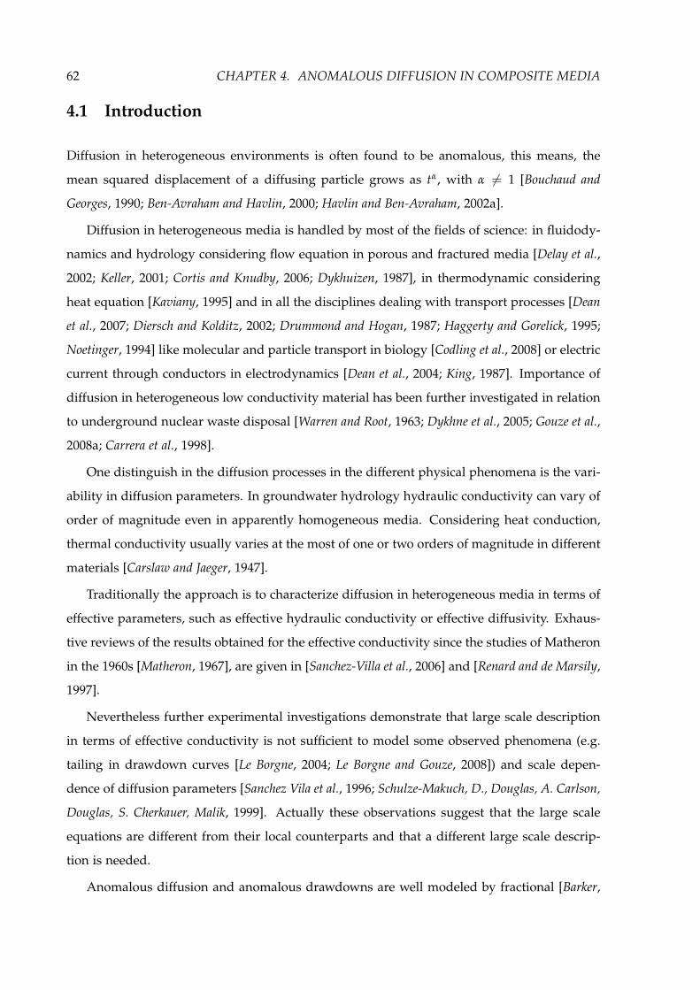
62 CHAPTER 4. ANOMALOUS DIFFUSION IN COMPOSITE MEDIA
4.1 Introduction
Diffusion in heterogeneous environments is often found to be anomalous, this means, the
mean squared displacement of a diffusing particle grows as tα, with α = 1 [Bouchaud and
Georges, 1990; Ben-Avraham and Havlin, 2000; Havlin and Ben-Avraham, 2002a].
Diffusion in heterogeneous media is handled by most of the fields of science: in fluidody-
namics and hydrology considering flow equation in porous and fractured media [Delay et al.,
2002; Keller, 2001; Cortis and Knudby, 2006; Dykhuizen, 1987], in thermodynamic considering
heat equation [Kaviany, 1995] and in all the disciplines dealing with transport processes [Dean
et al., 2007; Diersch and Kolditz, 2002; Drummond and Hogan, 1987; Haggerty and Gorelick, 1995;
Noetinger, 1994] like molecular and particle transport in biology [Codling et al., 2008] or electric
current through conductors in electrodynamics [Dean et al., 2004; King, 1987]. Importance of
diffusion in heterogeneous low conductivity material has been further investigated in relation
to underground nuclear waste disposal [Warren and Root, 1963; Dykhne et al., 2005; Gouze et al.,
2008a; Carrera et al., 1998].
One distinguish in the diffusion processes in the different physical phenomena is the vari-
ability in diffusion parameters. In groundwater hydrology hydraulic conductivity can vary of
order of magnitude even in apparently homogeneous media. Considering heat conduction,
thermal conductivity usually varies at the most of one or two orders of magnitude in different
materials [Carslaw and Jaeger, 1947].
Traditionally the approach is to characterize diffusion in heterogeneous media in terms of
effective parameters, such as effective hydraulic conductivity or effective diffusivity. Exhaus-
tive reviews of the results obtained for the effective conductivity since the studies of Matheron
in the 1960s [Matheron, 1967], are given in [Sanchez-Villa et al., 2006] and [Renard and de Marsily,
1997].
Nevertheless further experimental investigations demonstrate that large scale description
in terms of effective conductivity is not sufficient to model some observed phenomena (e.g.
tailing in drawdown curves [Le Borgne, 2004; Le Borgne and Gouze, 2008]) and scale depen-
dence of diffusion parameters [Sanchez Vila et al., 1996; Schulze-Makuch, D., Douglas, A. Carlson,
Douglas, S. Cherkauer, Malik, 1999]. Actually these observations suggest that the large scale
equations are different from their local counterparts and that a different large scale descrip-
tion is needed.
Anomalous diffusion and anomalous drawdowns are well modeled by fractional [Barker,

4.1. INTRODUCTION 63
1988; Acuna and Yortsos, 1995] and multi-fractional [de Dreuzy et al., 2010, 2004; Lods and Gouze,
2008] diffusion models. A limitation of these models is that the fractal dimension is not di-
rectly linked to the heterogeneity of the media, it can vary depending on the boundary and
initial conditions (e.g. [Little and Bloomfield, 2010; Zhang, 2004]). For these reasons interpreta-
tion of multi-fractal models is rather difficult [Tessier et al., 1996] and their utility for prediction
is limited [Labat et al., 2002].
CTRW has been successfully used to model non-Fickian transport in disordered media
e.g. [Berkowitz et al., 2006; Cortis, 2004; Gouze et al., 2008b; Sanchez-Villa et al., 2006; Metzler and
Klafter, 2000] and transient flow [Cortis and Knudby, 2006]. The equivalence between large scale
averaging theory and the CTRW has been object of the work of Noetinger et al. [Noetinger,
B.Estebenet and Quintard, 2001] and the equivalence between CTRW and multi rate mass trans-
fer (MRMT) models has been demonstrated by Dentz [Dentz and Berkowitz, 2003]. MRMT
models have been widely used to model transport and flow problems in heterogeneous me-
dia e.g. [Harvey and Gorelick, 1995; Carrera et al., 1998; Haggerty and Gorelick, 1995; Lods, 2004].
A particular CTRW in heterogeneous media, where the distribution of residence time de-
pends by the location, is called time domain random walk (TDRW). This method has been
first introduced by McCarthy [1993], used by Banton for simulating non-reactive solute trans-
port in d = 1 dimensional porous media [Banton et al., 1997], by Noetinger for the upscaling
of fluid flow in fracture rocks [Noetinger and Estebenet, 2000], and further developed by Delay
and Bodin [Delay et al., 2002; Bodin et al., 2003; Delay et al., 2005].
We consider diffusion in composite media. In particular we consider a dual and a multi
continuum model given in Figure 4.1. The dual continuum model is constituted by two
homogeneous layers which represent the mobile region (where the scalar quantity diffuses
faster) and the immobile region (where scalar quantity diffuses slower).
Since the pioneering ’double-porosity’ model of Barenblatt [Barenblatt et al., 1960] a large
number of double-permeability/porosity models have been developed (e.g. [Warren and Root,
1963; Dykhuizen, 1987; Peters and Klavetter, 1988; Dykhuizen, 1990; Bai et al., 1993]). These mod-
els assumes that both the mobile and the immobile zone are in quasi-equilibrium and mass
transfer is modeled as a first order process. Among others, works considering a kinetic ap-
proach are derived using perturbations methods [Zhang and Sun, 2000], or homogenization
method. Complete review of homogenized models for saturated conditions through a het-
erogeneous porous medium is given in [Peszynska and Showalter, 2007], while non-saturated
conditions are considered in [Lewandowska, 2004; Bertin et al., 2000].

64 CHAPTER 4. ANOMALOUS DIFFUSION IN COMPOSITE MEDIA
We take into account non-equilibrium effects in the immobile zone, which give raise to
anomalous behaviour and we derive temporally non-local governing equations.
Figure 4.1: On the left: dual continuum model, on the right: multi continuum model. Dual andmulti continuum model are constituted by a ’mobile’ layer of thickness dm and an immobile one ofthickness dim. Vertical arrows between the two layers indicate mass exchange between the mobile andthe immobile regions.
In the following we introduce the problem of diffusion in heterogeneous media, the
medium models taken into account and the numerical method used to test analytical solu-
tions. In the third section we derive non-local governing equation for the up-scaled dual
and the multi continuum model proposed. Successively we give the solutions for the model
derived focusing on anomalous behaviour of mean square displacement, first passage time
distribution and temporal evolution of the concentration and in the last section we focus on
the anomalous behaviour we can obtain with the model derived. Analytical solutions are
tested numerically. Main results are summed and discussed in the conclusions.
4.2 Diffusion in Heterogeneous Media
Diffusion of a scalar quantity C(x, t) in a heterogeneous medium is described by
R(x)∂C(x, t)
∂t−∇ · [K(x)∇C(x, t)] = 0. (4.1)
In the context of diffusion of contaminants in low conductivity media, R(x) can be related
to the medium porosity φ(x) and linear equilibrium adsorption properties of the medium
as R(x) = [1 − φ(x)]kd(x) + φ(x) with kd(x) the distribution coefficient, C(x, t) is the non-
adsorbed contaminant concentration, and K(x) the bulk diffusion coefficient. In the context of
heat transport, R(x) stands for heat capacity, C(x, t) temperature, and K(x) thermal conduc-
tivity. For the description of Darcy-scale flow in heterogeneous porous media, R(x) denotes
specific storativity, C(x, t) hydraulic head and K(x) hydraulic conductivity. This work is mo-
tivated through contaminant diffusion in low permeability media, and Darcy-scale flow by

4.2. DIFFUSION IN HETEROGENEOUS MEDIA 65
heterogeneous porous media.
4.2.1 Random Walk Perspective
The diffusion equation (4.1) is equivalent to the Langevin equation [Risken, 1989]
dx(t)dt
=∇K[x(t)]R[x(t)]
+
2K[x(t)]R[x(t)]
ξ(t), (4.2)
where x(t) denotes the trajectory of a particle, ξ(t) is a Gaussian white noise characterized by
zero mean and xi(t)ixi(t)j = δ(t− t) δij.
The scalar C(x, t) is expressed in terms of the particle trajectories x(t) as
C(x, t) = R(x)−1 δ[x− x(t)] , (4.3)
where the angular brackets denote the noise average.
The cases of variable conductivity K(x) and constant storativity R(x) = R, on the one
hand, and variable storativity R(x) and constant conductivity K(x) = K, on the other, can
be mapped into the random barrier and random trap models, respectively [Bouchaud and
Georges, 1990]. These models describe diffusion on random lattices. In the random barrier
model, each link of the lattice acts as a symmetrical barrier. For diffusion in a finite domain,
the equilibrium particle density is uniform and accumulation in low conductivity regions is
avoided [Bouchaud and Georges, 1990]. In the random trap model each lattice site is considered
a trap characterized by a random trapping time. In this model, the equilibrium distribution is
proportional to the distribution of trapping times [Bouchaud and Georges, 1990].
4.2.2 Numerical Simulations
Diffusion properties are spatially discontinuous in the proposed models, which makes the
use of (4.2) complicated because of the calculation of the gradient of the conductivity ∇K(x)
[Delay et al., 2005]. Therefore the method of choice is time domain random walk (TDRW),
which relies on spatial increments, whose absolute values are deterministic, combined with
random time increments [McCarthy, 1993; Banton et al., 1997; Delay et al., 2002]. We consider
the TDRW scheme presented in Dentz et al. [2012]. The TDRW that describes the random walk

66 CHAPTER 4. ANOMALOUS DIFFUSION IN COMPOSITE MEDIA
equivalent to eq. (4.1), used in the numerical simulations is:
xi(n + 1) = xj(n) + ξ ij, tn+1 = tn + θj, (4.4)
where the position of lattice point j is denoted by xj. The probability for a spatial transition
ξij between points j and i, wij, and the mean transition time τj are given by:
wij =bij
∑[ik] bkj, τj =
AjRj
∑[kj] bkj. (4.5)
where Aj is the area of the pixel j, ∑[ik] indicates the sum over the nearest neighbours of pixel
j and
bij =∆z,ij(K)ij
∆x, (4.6)
with (K)ij the harmonic mean of the conductivities of the two pixels i and j, ∆z,ij, the length
of the interface between the pixel i and j, given by the vertical discretization of the domain,
∆x the lag distance between the centres of the two pixels, or the horizontal discretization of
the domain that we take constant, so that the area of the pixel j is given by Aj = ∆x∆z,ij.
According to [Delay et al., 2002], we consider transition time exponentially distributed, and
the transition time density reads:
ψθj(θj) = τ−1j exp(−θj/τj). (4.7)
Details on the implementation of the numerical simulations are given in Appendix C.3.
4.2.3 Observables
4.2.3.1 Mean squared displacement
Diffusion in heterogeneous media can be characterized by the evolution of the mean-square
displacement (MSD) mij(t), which is defined by
mij(t) =
dx xixjc(x, t) = xi(t)xj(t). (4.8)
For normal diffusion, mij(t) evolves linearly in time mij(t) ∼ t. For diffusion in disordered
media this scaling is not valid in general, and it is often found that mij(t) ∼ tβ with β =
1 Bouchaud and Georges [1990]. For 0 < β < 1 the behavior is termed sub-diffusive, for β > 1,

4.3. MULTICONTINUUM MODEL 67
super-diffusive, and for β = 2 ballistic Havlin and Ben-Avraham [2002a]. Sub-diffusion in
disordered media is typically attributed to trapping in particular regions like dead ends and
bottlenecks that exist in the disordered structure.
4.2.3.2 First passage time distribution
Another quantity of interest is the first passage time distribution (FPTD) of a particle. The
information provided by the FPTD is central in many application ranging from contaminant
transport in geological media (solute breakthrough curves) Berkowitz et al. [2006], to the eval-
uation of reaction rates in diffusion limited reactions Havlin and Ben-Avraham [2002a], to name
a few. The FPTD f (x, t) can be defined by the renewal equation Hughes [1995]
C(x, t) = δ(x)δ(t) +t
0
dt f (x, t)C(x, t|x, t), (4.9)
where the propagator C(x, t|x, t) solves the diffusion equation (4.1) for the initial condition
C(x, t = t|x, t) = δ(x− x). In a d = 1 dimensional homogeneous medium, the FPTD scales
asymptotically as f (x, t) ∝ t−3/2.
4.2.3.3 Temporal evolution of the concentration
We will also consider the time evolution of C(x, t) at a given point in space, which in the con-
text of Darcy flow in heterogeneous media is termed drawdown Delleur [1999]. The drawdown
depends on the boundary and initial conditions. For an instantaneous point-like injection into
a d-dimensional homogeneous medium, it scales asymptotically as C(x, t) ∝ t−d/2.
4.3 Multicontinuum Model
4.3.1 Model Medium and Governing Equations
The heterogeneous model medium under consideration is a d = 2 dimensional composite
medium that consists of a mobile, highly conductive layer and a (heterogeneous) immobile,
low conductivity layer, as illustrated in Figure 4.1. For diffusion in this medium, equation (4.1)
can be separated into an equation for the mobile region and one for the immobile region. The
coordinate vector now and in the following denotes x = (x, z)T. Thus, for the mobile regions

68 CHAPTER 4. ANOMALOUS DIFFUSION IN COMPOSITE MEDIA
dim ≤ z ≤ d, we obtain
Rm∂Cm(x, t)
∂t− Km∇2Cm(x, t) = 0, (4.10)
where we defined cm(x, t) = c(x, t) for dim ≤ z ≤ d. In the immobile region 0 ≤ z ≤ dim,
diffusion is described by
Rim(x)∂Cim(x, t)
∂t− Kim(x)∇2Cim(x, t) = 0. (4.11)
The immobile Cim(x, t) is defined analogously by Cim(x, t) = C(x, t) for 0 ≤ z ≤ dim. Conti-
nuity of C(x, t) and flux −K(x)∇C(x, t) are imposed at the interface between the mobile and
immobile layers, at z = dim [Carslaw and Jaeger, 1947], so that at z = dim
Cm(x, t) = Cim(x, t), Km∂Cm(x, t)
∂z= Kim(x)
∂Cim(x, t)∂z
. (4.12)
In the following, we assume no flux conditions at the horizontal boundaries,
Km∂Cm(x, t)
∂z
z=d
= 0, Kim(x)∂Cim(x, t)
∂z
z=0
. (4.13)
Diffusion occurrs in multiple connected continua. Dual continuum models can be divided
into ’double permeability’ and ’double porosity’ models [Zhang and Sun, 2000]. In some ’dual
porosity’ models the immobile regions are constrained to communicate only with the mo-
bile region and mass transfer between the immobile regions is neglected by default. Multi-
continuum model that prevent mass transfer between immobile regions are also termed in
literature ’comb models’ [Havlin and Ben-Avraham, 2002a; Bouchaud and Georges, 1990; Dvoret-
skaya and Kondratenko, 2009].
Here, we assume that the conductivity Km in the mobile layer is much larger than the
maximum conductivity in the immobile layers, Km maxx∈RKim(x). This condition allows
to overcome the distinction between ’double permeability’ and ’double porosity’ models, be-
cause the difference in the conductivity between the mobile and the immobile zone makes, by
itself, horizontal diffusion in the immobile layer negligible. Referring to Figure 4.1, double (or
multi) porosity models neglect horizontal diffusion in the immobile layer and immobile zones
act as source terms for the mobile zone.
The simplest multi-continuum model is constituted by the coupling of two homogeneous

4.3. MULTICONTINUUM MODEL 69
regions. The pioneering double permeability model of Barenblatt et al. [Barenblatt et al., 1960]
models flow through fractured media. In such media, flow takes place essentially only in the
fractures. However, fluid may be transferred into the immobile matrix and then after a certain
time back into the fractures.
In the multi continuum model, heterogeneity of the immobile layer is characterized by
spatially variable bulk immobile conductivity defined by κ(x) = χimKim(x) and spatially vari-
able bulk retardation factor defined by ρ(x) = χimRim(x). We handle spatial heterogeneity
in a stochastic framework. In a stochastic framework a medium is considered as a particular
realization of an ensemble of media with the same statistical properties and spatially vary-
ing conductivity and retardation factor are modeled as spatial random fields. We consider a
stationary and ergodic medium, with a finite correlation. Considering an observation scale
far larger than the correlation scale, we can approximate the medium organization in bins,
where diffusion properties in each bins are independent. Thus, such medium can be com-
pletely defined by a single point distribution of the diffusion parameters. A schema of the
model is given in Figure 4.1. Referring to the figure heterogeneity of the immobile layer is
organized in bins. At each bin is assigned independently a random bulk cinductivity taken
from a distribution pκ(κ) and a random bulk retardation taken from a distribution pρ(ρ).
4.3.2 Vertical Average
In the following, we derive the governing equations for the average mobile particle distribu-
tion cm(x, t), which is defined as
cm(x, t) =1
dm
d
dim
dz Cm(x, t). (4.14)
Averaging of (4.10) over the vertical gives for cm(x, t)
Rm∂cm(x, t)
∂t− Km
∂2cm(x, t)∂x2 = −Kim(x)
dm
∂Cim(x, t)∂z
z=dim
, (4.15)
where we used the flux continuity condition (4.12) and the boundary conditions (4.13). Conti-
nuity in c(x, t) at the interface defines the boundary condition for the diffusion problem (4.11)
in the immobile region. The system of equations (4.11) and (4.15) can be closed as follows.
In the model medium under consideration, the conductivity Km in the mobile layer is much
larger than the maximum conductivity in the immobile layers, Km maxx∈R[Kim(x)]. This

70 CHAPTER 4. ANOMALOUS DIFFUSION IN COMPOSITE MEDIA
assumption has two effects on the dynamic of the model: (i) the concentration in the mo-
bile zone equilibrates much faster that the one in the immobile zone, (ii) mass transfer in the
immobile zone is sub-leading compared to the mass transfer in the mobile layer.
These processes are controlled by the characteristic time scales for vertical diffusion in the
mobile and immobile layers, defined by
τm =d2
mRm
Km, τim(x) =
d2imRim(x)Kim(x)
. (4.16)
Considering τm minx∈R[τim(x)] the distribution Cm(x, t) in the mobile layer will equilibrate
much faster than Cim(x, t) in the immobile layers. Consequently, at observation times much
larger than τm, we can approximate
Cm(x, t) ≈ cm(x, t). (4.17)
Considering mass transfer in the immobile layer, the condition Km maxx∈R[Kim(x)] makes
horizontal diffusion in the immobile layer negligible for two inter-related reasons. Firstly be-
cause transition time in the immobile layer is far larger than in the mobile layer and horizontal
diffusion in the immobile layer is slower respect horizontal diffusion in the mobile layer. Sec-
ondly because, in a particle tracking framework, the probability for a particle in the immobile
layer to move in the mobile zone is far higher respect the probability to move horizontally in
the immobile layer.
Thus, we disregard horizontal diffusion in the immobile layers. Based on these assump-
tions, we can approximate the diffusion problem (4.11) in the immobile layer by
Rim(x)∂Cim(x, t)
∂t− Kim(x)
∂2Cim(x, t)∂z2 = 0, (4.18)
with the boundary conditions
Cim(x, t)|z=dm= cm(x, t), Kim(x)
∂Cim(x, t)∂z
z=0
= 0. (4.19)
These assumptions are validated using particle tracking simulations.
From (4.18), we obtain by vertical integration for the boundary flux term on the right side

4.3. MULTICONTINUUM MODEL 71
of (4.15)
−Kim(x)dm
∂Cim(x, t)∂z
z=dim
= Rim(x)dimdm
∂cim(x, t)∂t
, (4.20)
where we defined the average immobile concentration
cim(x, t) =1
dim
dim
0
dz Cim(x, t). (4.21)
The diffusion problem (4.18)–(4.19) can be solved explicitly in Laplace space, see Appendix
C.2. The Laplace transform is defined in Abramowitz and Stegun [1965]. Laplace transformed
quantities are denoted here by a tilde, λ is the Laplace variable. In Appendix C.2, we derive
for the average immobile concentration
cim(x, t) =t
0
dtg[t− t|τim(x)]cm(x, t)− cim(x, 0)t
0
dtg[t− t|τim(x)] + cim(x, 0). (4.22)
The memory function g[t|τim(x)] is defined in terms of its Laplace transform as
g∗[λ|τim(x)] =1
λτim(x)tanh
λτim(x)
. (4.23)
The memory function depends on the properties of the immobile region only and it is an
intrinsic characteristic of the medium. Figure 4.2 shows the inverse Laplace transform (5.32)
for a given position x. In this work Laplace inversion is computed numerically using a Matlab
function for numerical inversion by the Hoog algorithm [Hollenbeck, 1998].

72 CHAPTER 4. ANOMALOUS DIFFUSION IN COMPOSITE MEDIA
10 110 2 100 102101 103
102
10 2
10 6
t
g(t)
im = 1
im = 10
im = 102
Figure 4.2: Memory function g[t|τim] for an homogeneous immobile zone plotted in function of timefor different values of Kim in double logarithmic scale. Parameters: Rm = 1, Rim = 1, dm = 1, dim =1, Km = 100, Kim = 1, 10−1 and 10−2. Vertical dashed lines indicate the characteristic timescalesgiven by the characteritic times of the immobile zones for the different curves: τim = 1, 10 and 102.
The function g[t|τim] decrease as t−1/2 for time smaller than the characteristic time of the
immobile layer τim and then, once the immobile region is in equilibrium, it decreases to zero
exponentially.
Combining (4.22) with (4.20) and using the resulting expression in (4.15), we obtain for the
vertically averaged mobile density cm(x, t) the closed equation
ρm∂cm(x, t)
∂t+
∂
∂t
t
0
dtϕ(t− t|x)cm(x, t) = κm∂2cm(x, t)
∂x2 + cim(x, 0)ϕ(t|x). (4.24)
We define the mobile and immobile volume fractions by χm = dm/d and χim = dim/d and
the bulk retardation ρm = χmRm and the bulk diffusion κm = χmKm coefficient. The memory
function ϕ(t|x) is defined by
ϕ(t|x) = ρim(x)g[t|τim(x)], (4.25)
with the bulk immobile retardation coefficient ρim(x) = χimRim(x). We also define the
bulk immobile diffusion κim = χimKim(x), thus the characteristic immobile diffusion time
is τim(x) = d2imρim(x)/κim(x). The total upscaled concentration c(x, t) comprehensive of the
contribution of the mobile and the immobile region, is given by:
c(x, t) =1d
d
0C(x, t) dz = χmcm(x, t) + χimcim(x, t). (4.26)
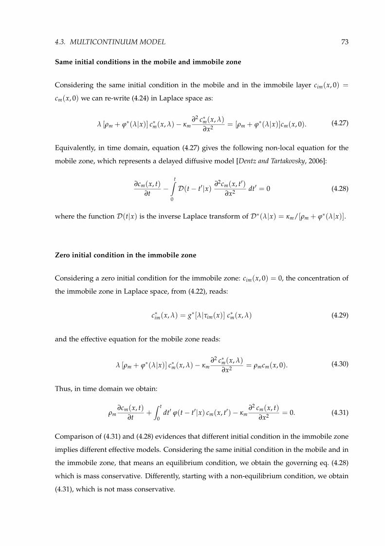
4.3. MULTICONTINUUM MODEL 73
Same initial conditions in the mobile and immobile zone
Considering the same initial condition in the mobile and in the immobile layer cim(x, 0) =
cm(x, 0) we can re-write (4.24) in Laplace space as:
λ [ρm + ϕ∗(λ|x)] c∗m(x, λ)− κm∂2 c∗m(x, λ)
∂x2 = [ρm + ϕ∗(λ|x)]cm(x, 0). (4.27)
Equivalently, in time domain, equation (4.27) gives the following non-local equation for the
mobile zone, which represents a delayed diffusive model [Dentz and Tartakovsky, 2006]:
∂cm(x, t)∂t
−t
0
D(t− t|x)∂2cm(x, t)
∂x2 dt = 0 (4.28)
where the function D(t|x) is the inverse Laplace transform of D∗(λ|x) = κm/[ρm + ϕ∗(λ|x)].
Zero initial condition in the immobile zone
Considering a zero initial condition for the immobile zone: cim(x, 0) = 0, the concentration of
the immobile zone in Laplace space, from (4.22), reads:
c∗im(x, λ) = g∗[λ|τim(x)] c∗m(x, λ) (4.29)
and the effective equation for the mobile zone reads:
λ [ρm + ϕ∗(λ|x)] c∗m(x, λ)− κm∂2 c∗m(x, λ)
∂x2 = ρmcm(x, 0). (4.30)
Thus, in time domain we obtain:
ρm∂cm(x, t)
∂t+
t
0dt ϕ(t− t|x) cm(x, t)− κm
∂2 cm(x, t)∂x2 = 0. (4.31)
Comparison of (4.31) and (4.28) evidences that different initial condition in the immobile zone
implies different effective models. Considering the same initial condition in the mobile and in
the immobile zone, that means an equilibrium condition, we obtain the governing eq. (4.28)
which is mass conservative. Differently, starting with a non-equilibrium condition, we obtain
(4.31), which is not mass conservative.

74 CHAPTER 4. ANOMALOUS DIFFUSION IN COMPOSITE MEDIA
The total concentration in function of the concentration in the mobile zone is:
c∗(x, λ) = χm + χimg∗[λ|τim(x)] c∗m(x, λ). (4.32)
In the following, we distinguish between the dual continuum model, consisting of a high
and low conductivity layer and the multi continuum model characterized by spatially varying
diffusion proprieties in the immobile layer. In order to investigate the diffusion behavior in
the multi-continuum medium, we will further average Equation (4.24) over the distribution of
the diffusion properties in the heterogeneous low conductivity layer.
4.3.3 Ensemble Average
In order to obtain an upscaled effective formulation, we average the effective governing equa-
tions (4.24) and (4.22) horizontally over the immobile zone. Ensemble average over the het-
erogeneity of the immobile zone of equations (4.24) gives:
ρm∂cm(x, t)
∂t+
∂
∂t
t
0
dtϕ(t− t|x) cm(x, t) = κm∂2cm(x, t)
∂x2 + cim(x, 0)ϕ(t|x). (4.33)
where the overbar indicates ensemble average. In the last term of eq. (4.33), the initial condi-
tion cim(x, 0) is deterministic and therefore we can break ensemble average:
cim(x, 0)ϕ(t|x) = cim(x, 0)ϕ(t|x). (4.34)
We define a global memory function ϕ(t) given by the ensemble average of the local memory
functions ϕ(t|x) given in (4.25) associated at each immobile zone:
ϕ(t) = ϕ(t|x). (4.35)
The average can be executed explicitly and we obtain:
ϕ(t) = ρ(x)g[t|τ(x)] =
dρ
dτ pρ,τ(ρ, τ) ρ g(t|τ), (4.36)
where pρ,τ(ρ, τ) is the joint distribution of the variable ρ and τ. In order to further develop
equation (4.36), we consider the expression for g∗(λ|τ) given in (5.32) and we notice that
g∗(λ|τ) is precisely function of the product λτ. This implies that g(t|τ) can be expressed in

4.3. MULTICONTINUUM MODEL 75
function of the single variable function g(t/τ) as:
g(t|τ) =1τ
g
tτ
(4.37)
where g(t) ≡ g(t|1) is the inverse Laplace transform of g∗(λ) ≡ g∗(λ|1). Thus, Eq. (4.36) can
be re-written as:
ϕ(t) = ρ(x)g[t|τ(x)] =
dρ
dτ pρ,τ(ρ, τ)ρ
τg
tτ
. (4.38)
The joint distribution pρ,τ(ρ, τ) of Eq. (4.38) can be expressed by using of Bayes’ theorem as:
pρ,τ(ρ, τ) = pρ(ρ) pτ(τ|ρ), (4.39)
and the conditional distribution pτ(τ|ρ) is defined in terms of the distribution of conductivity
pκ(κ) as:
pτ(τ|ρ) =d2
imρ
τ2 pκ
d2
imρ
τ
. (4.40)
Back to the ensemble average over the governing equation of the mobile zone, considering the
second term of eq. (4.33) we have a problem of closure. We close the equation by a mean field
approximation:
ϕ(t− t|x) cm(x, t) ≈ ϕ(t|x) cm(x, t). (4.41)
Thus we obtain the following upscaled equation for the average mobile concentration:
ρm∂cm(x, t)
∂t+
∂
∂t
t
0
dtϕ(t− t) cm(x, t) = κm∂2cm(x, t)
∂x2 + cim(x, 0)ϕ(t). (4.42)
In order to obtain an upscaled expression for cim(x, t) we average eq. (4.22) and we have:
cim(x, t) =t
0
dt g[t− t|τ(x)] cm(x, t)−t
0
dtcim(x, 0)g[t− t|τ(x)] + cim(x, 0). (4.43)
The initial value cim(x, 0) is deterministic so that the last average in the previous equation
does not represent a closure problem. The closure problem given by g[t− t|τ(x)] cm(x, t) is

76 CHAPTER 4. ANOMALOUS DIFFUSION IN COMPOSITE MEDIA
closed, as for (4.33), using mean field approximation. Thus we obtain:
cim(x, t) =t
0
dt g(t− t) cm(x, t)− cim(x, 0)t
0
dtg(t− t) + cim(x, 0) (4.44)
where we defined:
g(t) = g[t|τ(x)] = ∞
0pτ(τ) g(t|τ) dτ. (4.45)
The total concentration c(x, t) is obtain from averaging of (4.26) and we easily obtain:
c(x, t) = χmcm(x, t) + χimcim(x, t). (4.46)
Although the characterised time τ(x) depends on the ratio between the bulk retardation ρim(x)
and the bulk conductivity κim(x), the dynamic of system characterized by spatially variable
conductivity or spatially variable retardation factor is very different. Indeed a variable con-
ductivity model corresponds to a barrier model, while a model with a space dependent re-
tardation factor can be mapped into a trap model [Havlin and Ben-Avraham, 2002a]. For this
reason in the following we consider the two cases separately and indeed we obtain differ-
ent results. We consider the two cases: (i) constant ρim = ρ0, variable κim and (ii) constant
κim = κ0, variable ρim.
4.3.3.1 Constant retardation factor
In the case of constant ρim = ρ0 and variable κim(x), the distribution of the retardation factor
can be written as pρ(ρ) = δ(ρ− ρ0), so that the joint distribution in (4.38) is given by:
pρ,τ(ρ, τ) = δ(ρ− ρ0) pτ(τ|ρ) (4.47)
and the marginal distribution of the characteristic times of the immobile zone τ in function of
the distribution of the conductivity pκ(κ) reads:
pτ(τ) =d2
imρ0
τ2 pκ
d2
imρ0
τ
. (4.48)
Substituting (4.47) in the expression for the global memory function given in (4.38), we have:
ϕκ(τ) = ρ0
dτ pτ(τ)
1τ
g
tτ
, (4.49)

4.3. MULTICONTINUUM MODEL 77
where the subscript κ of the memory function indicates that it refers to a distribution of bulk
conductivity. Considering the change of variable y = t/τ in the previous equation, we obtain:
ϕκ(t) = ρ0
dy
1y
pτ
ty
g (y) . (4.50)
The previous equation indicates that the temporal behaviour of the memory function ϕκ(t) is
determined by the distribution of the characteristic time of the immobile zone pτ(τ). Com-
paring the definition of ϕκ(t) given in (4.49) and the definition of g(t), given in (4.45), and
considering the relation between g(t) and g(t/τ) given in (4.37), we see that for a constant
retardation factor ρ0 we have:
g(t) =ϕκ(t)
ρ0. (4.51)
4.3.3.2 Constant conductivity
In the case of constant bulk conductivity κim = κ0 in the immobile zone and spatially variable
retardation factor ρim(x), the joint distribution in (4.38) is:
pρ,τ(ρ, τ) = pρ(ρ) δ
τ −
d2imρ
κ0
. (4.52)
Consequently, the marginal distribution of the characteristic times results:
pτ(τ) =
dρ pρ(ρ) δ
τ −
d2imρ
κ0
=
κ0
d2im
pρ
τκ0
d2im
(4.53)
and the memory function for the multi continuum model with variable retardation factor is:
ϕρ(t) =κ0
d2im
dτ pτ(τ) g
tτ
. (4.54)
where the subscript ρ indicates that the memory function refers to a distribution of bulk
retardation factor. Considering the same change of variable y = t/τ as in (4.49), we obtain:
ϕρ(t) =κ0
d2im
dy
ty2 pτ
tτ
g (y) . (4.55)
Comparing the memory functions for the case of variable conductivity, given in (4.50), and
variable retardation factor, given in (4.55), we notice that in both cases the temporal behaviour
of the memory function depends on the distribution of the characteristic time of the immobile

78 CHAPTER 4. ANOMALOUS DIFFUSION IN COMPOSITE MEDIA
zone pτ(τ), but the same distribution of characteristic times determines different scaling of
the memory function, because the integrands are different.
4.3.4 Dual Continuum Model
In the following we consider a dual continuum model characterized by a homogeneous immo-
bile zone. The model is similar to the well known comb models for diffusion in disordered me-
dia [Havlin and Ben-Avraham, 2002a]. Anomalous behaviour in comb model has been already
studied. Metzler and Klafter [2000] studied sub-diffusion in comb model by particle tracking
methods and Arkhincheev [2000] deduced an exact solution for a generalized diffusion equa-
tion taking into account a random disappearance and birth of the diffusion particles. More
recently Dvoretskaya and Kondratenko [2009] studied anomalous subdiffusion in comb models
considering an infinite immobile zone and Iomin [2011] derived subdiffusion in fractal comb.
We present the dual continuum model as a particular case of the multi continuum model.
The simpler dual continuum model enables us to discuss some basic feature of the proposed
model. Considering an homogeneous immobile layer characterized by a bulk conductivity κim
and a bulk retardation factor ρim, the joint distribution in the equation of the global memory
function (4.36) is:
ρρ,τ(ρ, τ) = δ(ρ− ρim) δ(τ − τim) (4.56)
with τim = d2imρim/κim. Thus the memory function g(t) defined in (4.45) and the global
memory function ϕ(t) defined in (4.36) depend on time only. In Laplace space, the memory
function for the dual continuum model, substituting (4.56) in (4.36) and considering (5.32)
with τim(x) ≡ τim, reduces to:
ϕ∗(λ) = ρim1√
λτimtanh
λτim. (4.57)
Clearly, Eq.(4.57) can be also obtained directly from (4.25) and (5.32) considering a constant
retardation factor ρim(x) = ρim and characteristic time τim(x) = τim.
In the derivation of the multi continuum model we assumed mean ergodicity. In Appendix
C.3 is briefly discussed the error we commit considering ensemble average instead of spatial
average. In the special case of the dual continuum model the fact that we do not need ensemble
average over the immobile zone (because it is homogeneous) implies less assumptions in the
derivation proposed.

4.4. DIFFUSION BEHAVIOUR 79
4.4 Diffusion Behaviour
We discuss the diffusion behaviour of the multi continuum model derived in the previous
section using explicit Laplace solutions and numerical simulations. We take into consideration
the mobile concentration of the mobile zone cm(x, t), its mean squared displacement (MSD)
and its first passage time distribution (FPTD). Explicit analytical solutions are given in Laplace
space and temporal behaviour shown in the figures are obtained by numerical inversion of
the solution in Laplace space by using the Hoog algorithm [Hollenbeck, 1998]. Numerical
simulation are performed using the TDRW scheme presented in Section 4.2.2. For brevity we
do not give the solutions for cim(x, t) and c(x, t) that can be easily derived from cm(x, t) by
considering (4.44) and (4.46).
4.4.1 Solutions
Here we give analytical solutions in Laplace space for cm(x, t), its MSD and its FPTD for the
dual and the multi composite models.
4.4.1.1 Mobile concentration cm(x, t)
As initial condition for the mobile zone, we consider a pulse injection in the origin. We model
it as an instantaneous imposed value c0 over an infinitesimal distance d0, centered in x = 0
cm(x, 0) = c0d0δ(x), (4.58)
where δ(x) is the delta function and in case of a finite volume representation d0 can be given by
the discretization of the system. Note that the product c0d0 represents the total mass injected
in the system. Considering in the immobile zone the same initial condition cim(x, 0) = cm(x, 0),
the solution of (4.42) is:
c∗m(x, λ) =
ρm + ϕ∗(λ)
4 κm λe−
λ [ρm+ϕ∗(λ)]
κm |x|, (4.59)
where, for the dual continuum model the memory function ϕ(t) is given in (4.57) and for the
multi continuum model with spatially variable conductivity ϕ(t) ≡ ϕκ(t) given by (4.49) and
for spatially variable retardation factor ϕ(t) ≡ ϕρ(t) given in (4.54).

80 CHAPTER 4. ANOMALOUS DIFFUSION IN COMPOSITE MEDIA
4.4.1.2 Mean square displacement
In the following we consider the MSD defined in (4.8) for the mobile concentration. In Laplace
space the definition of the MSD given in (4.8) is:
m∗2(λ) =
∞
−∞x2 c∗m(x, λ) dx. (4.60)
Substituting in the previous equation the expression for cm(x, λ) given in (5.29) we obtain:
m∗2(λ) =
2 κm
λ2 [ρm + ϕ∗(λ)] (4.61)
where, as before the memory function ϕ(t) for the dual continuum model is given in (4.57)
and for the multi continuum model in (4.49) for variable conductivity and in (4.54) for variable
retardation factor.
4.4.1.3 First passage time distribution
According to the definition of Risken [1989], the FPTD f (t) for the mobile concentration cm(x, t)
is defined as:
f (t) = − xc
−∞
∂cm(x, t)∂t
dx. (4.62)
where xc is the control point where the FPTD is computed. Considering the effective ex-
pression for cm(x, t) given in (4.28) for the same initial conditions in the mobile and in the
immobile zone, the FPTD reads:
f (t) = − xc
−∞
∞
0D(t− t)
∂2cm(x, t)∂x2 dtdx. (4.63)
where D(t) = D(t|x). Equivalently in Laplace space we have D∗(λ) = κm/[ρm + ϕ∗(λ)] and
executing the integral respect to the space variable, Eq. (4.63) reads:
f ∗(λ) =κm
ρm + ϕ∗(λ)∂c∗m(x, λ)
∂x
x=xc
. (4.64)
Substituting in the previous equation the solution of c∗m(x, λ) given in (5.29), the FPTD in
Laplace space results:
f ∗(λ) =12
e−
λ [ρm+ϕ∗(λ)]κm |xc| (4.65)
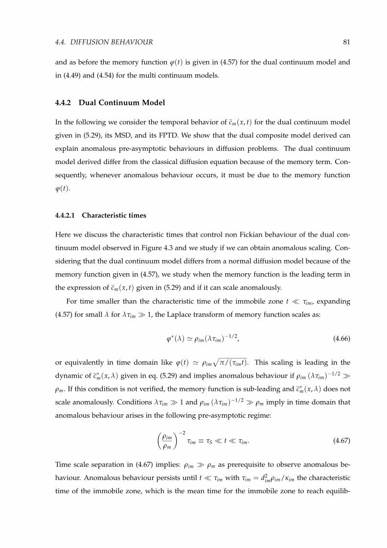
4.4. DIFFUSION BEHAVIOUR 81
and as before the memory function ϕ(t) is given in (4.57) for the dual continuum model and
in (4.49) and (4.54) for the multi continuum models.
4.4.2 Dual Continuum Model
In the following we consider the temporal behavior of cm(x, t) for the dual continuum model
given in (5.29), its MSD, and its FPTD. We show that the dual composite model derived can
explain anomalous pre-asymptotic behaviours in diffusion problems. The dual continuum
model derived differ from the classical diffusion equation because of the memory term. Con-
sequently, whenever anomalous behaviour occurs, it must be due to the memory function
ϕ(t).
4.4.2.1 Characteristic times
Here we discuss the characteristic times that control non Fickian behaviour of the dual con-
tinuum model observed in Figure 4.3 and we study if we can obtain anomalous scaling. Con-
sidering that the dual continuum model differs from a normal diffusion model because of the
memory function given in (4.57), we study when the memory function is the leading term in
the expression of cm(x, t) given in (5.29) and if it can scale anomalously.
For time smaller than the characteristic time of the immobile zone t τim, expanding
(4.57) for small λ for λτim 1, the Laplace transform of memory function scales as:
ϕ∗(λ) ρim(λτim)−1/2, (4.66)
or equivalently in time domain like ϕ(t) ρim
π/(τimt). This scaling is leading in the
dynamic of c∗m(x, λ) given in eq. (5.29) and implies anomalous behaviour if ρim (λτim)−1/2
ρm. If this condition is not verified, the memory function is sub-leading and c∗m(x, λ) does not
scale anomalously. Conditions λτim 1 and ρim (λτim)−1/2 ρm imply in time domain that
anomalous behaviour arises in the following pre-asymptotic regime:
ρimρm
−2τim ≡ τS t τim. (4.67)
Time scale separation in (4.67) implies: ρim ρm as prerequisite to observe anomalous be-
haviour. Anomalous behaviour persists until t τim with τim = d2imρim/κim the characteristic
time of the immobile zone, which is the mean time for the immobile zone to reach equilib-

82 CHAPTER 4. ANOMALOUS DIFFUSION IN COMPOSITE MEDIA
rium by diffusion along the vertical direction. For λτim 1 the Laplace transform of memory
function given in (4.57) tends to the constant value:
limλτ1
ϕ∗(λ) ρim. (4.68)
Thus, asymptotically, for t τim the double continuum system acts as an equivalent homo-
geneous one with ϕ∗(λ) ρim.
Anomalous behaviour starts, as indicated in (4.67), for time larger than a characteristic
time that we called τS. In order to give a physical meaning to the characteristic time τS, we
call dz the penetration length of mass solute into the immobile layer by diffusion after time
t = τS, so that τS = d2z Rim/Kim. Therefore condition in (4.67), t τS, can be re-written as:
dzRim dmRm. The previous condition indicates that the amount of mass that has entered
into the immobile zone after time τS is bigger than the amount of mass into the mobile one.
For time smaller than τS, diffusion takes place basically only into the mobile layer and the
contribution of the immobile one is negligible. After the time τS enough solute mass entered
the immobile zone, its contribution is relevant in the dynamic of the system and the scaling
term of the memory function induces anomalous scaling in cm(x, t).
In the following we derive and discuss the anomalous scaling for cm(x, t), its MSD and its
FPTD observable in the pre-asymptotic regime given (4.67) considering the condition ρim
ρm.
4.4.2.2 Mobile concentration cm(x, t)
We consider temporal evolution of cm(x, t) given by inverse Laplace transform of (5.29). Fig-
ure 4.3 shows the temporal evolutions of cm(x, t) for the dual continuum medium obtained
analytically from eq. (5.29) and numerically using the TDRW particle tracking. We notice that
curves associated at different characteristic times of the immobile zone τim behave differently
for time t < τim. For time t > τim the system behaves as an equivalent homogeneous one and
all the curves scale as cm(x, t) ∼ t−1/2, as in a normal diffusion.

4.4. DIFFUSION BEHAVIOUR 83
100 101 102 103
10 2
t
c m(x
,t)
DC, Kim:10 1
DC, Kim:10 2
DC, Kim:10 3
~ t 1/2
imimp,m
Figure 4.3: Temporal evolution of cm(x, t) for the dual continuum model using the analytical solutiongiven in (5.29) and numerical simulaitons for different values of the conductivity of the immobile layerKim = 10−1, 10−2, 10−3. Parameters: observation point x = 5, Rm = 1, Rim = 1, dm = 2, dim = 2,Km = 10. Vertical dashed lines indicate the peak mean arrival time τp,m = x2Rm/Km due to diffusionin the mobile layer, common for all the curves, and τim = d2
imRim/Kim are the characteristic times of theimmobile zone related to the different curves. Parameters numerical simulation: horizontal and verticaldiscretization: ∆x = ∆z = 0.5, number of particles: np = 5 ∗ 106.
Anomalous scaling of the mobile concentration is obtained subtituting the temporal scaling
of the memory function given in (4.66) in the solution for cm(x, t) given in (5.29) and expanding
the obtained equation for λτim 1, we obtain
c∗m(x, λ)
ρimτ−1/2
im4κm
λ−3/4. (4.69)
Equivalently, considering the inverse Laplace transform of the previous equation, we derive
that the dual continuum model in time domain gives the following sub-diffusive anomalous
scaling:
cm(x, t) 12 Γ(3/4)
ρimκim
d2imκ2
m
1/4t−1/4, (4.70)
where Γ(·) is the gamma function. Figure (4.4) displays inverse Laplace transform of c∗m(x, λ)
given in (5.29) focusing on the anomalous behaviour. Analytical solution istested using nu-
merical simulation. Temporal evolution of cm(x, t) scales anomalously as t−1/4, as derived in
(4.70), for time smaller than τim, and then scales as in a homogeneous medium as t−1/2. The
time that corresponds to the peak in the temporal evolution of the concentration, τp,m, is given
by the diffusion parameters of the mobile zone τp = x2ρm/κm with x the distance of the obser-
vation point. The first characteristic time τS given in (4.67), which indicates when anomalous

84 CHAPTER 4. ANOMALOUS DIFFUSION IN COMPOSITE MEDIA
100 101 102 103 10410 3
10 2
10 1
t
c m(x
,t)
DC modelTDRW
~ t 1/2~ t 1/4
imp,m
Figure 4.4: Temporal evolution of cm(x, t) using the analytical solution given in (5.29) and TDRWsimulaiton. Parameters: Km = 10, Kim = 10−2, dm = 0.1, dim = 10, Rm = 1, Rim = 1, x = 10.Dash lines: normal behaviour cm(t) ∼ t−1/2, anomalous subdiffusive behaviour cm(t) ∼ t−1/4, meanpeak arrival time due to the diffusion parameter of the mobile zone τp,m = x2Rm/Km, characteritistime of the immobile zone to reach equilibrium τim = d2
imRim/Kim. Parameters numerical simulation:horizontal discretization: ∆x = 1, vertical discretization: ∆z = 0.5, number of particles: np = 106.
behavior starts, is smaller than τp,m and therefore we observe anomalous behaviour straight
after τp,m.
4.4.2.3 Mean square displacement
Substituting the anomalous scaling of the memory function given in (4.66) in the solution for
the MSD given in (4.61) we have:
m∗2(λ) 2κm
ρimτ−1/2im
λ−3/2, (4.71)
which in time domain results:
m2(t) 4κm
τim
π ρ2im
t1/2. (4.72)
The MSD increases with the square root of time, which indicates a sub-diffusive behaviour.
Asymptotically the memory function ϕ∗(λ) ρim (see (4.68)) and therefore, considering the
inverse Laplace transform of (4.61), with ϕ∗(λ) constant, the MSD grows linearly with time as
in a classical diffusion problem: m2(t) ∼ t.
Figure 4.5 shows the MSD given in (4.61) and TDRW numerical simulations, focusing on
anomalous behaviour. We observe that for time smaller than τim the MSD increases with time

4.4. DIFFUSION BEHAVIOUR 85
as t1/2 and for time larger than τim it increases linearly with time.
100 101 102 103103
104
105
106
t
MSD
DC modelTDRW DPermTDRW DPor
~ t1/2
~ t
im
Figure 4.5: Mean square displacement for the dual continuum model. Numerical simulation arepreformed blocking by default horizontal diffusion in the immobile layer (as in ’double porosity’ models)and without blocking by default horizontal diffusion in the immobile layer (as in ’double permeability’models). Parameters: κm = 10, κim = 10−2, dm = 1, dim = 1, ρm = 10−3, ρim = 1.
4.4.2.4 First passage time distribution
Considering the anomalous scaling of the memory function given in (4.66) in the expression
for the FPTD given in (4.65) we obtain:
f ∗(λ) =12
e−
τ−1/2imκm λ1/4|xc|, (4.73)
which corresponds to a Levy stable distribution. Expanding the previous equation for small λ
and using the Tauberian theorem, we obtain that FPTD in time domain scales as f (t) ∼ t−5/4.
Asymptotically, as stated before, ϕ∗(λ) = ρim and the FPTD in time domain results:
f (t) 12
ρm + ρim
4 κmπ|xc|
e−ρm+ρim
4κm t x2c
t3/2 . (4.74)
Expanding the previous equation for large times FPTD scales as f (t) ∼ t−3/2, which corre-
sponds to the normal scaling of the FPTD for normal diffusion in d = 1 spatial dimensional
medium. Figure 4.6 illustrates the anomalous scaling of the FPTD for the double continuum
model. In the figure is highlighted the pre-asymptotic anomalous scaling as f (t) ∼ t−5/4 till
τim and the normal scaling as f (t) ∼ t−3/2 for larger time.
Scaling of temporal evolution, mean square displacement and first passage time distribu-

86 CHAPTER 4. ANOMALOUS DIFFUSION IN COMPOSITE MEDIA
10 4 10 2 100 102
10 10
10 5
100
t
FPTD
DC model
~ t 3/2
~ t 5/4
im
Figure 4.6: First passage time distribution for the double continuum model. Parameters: xc = 10,Rm = 0.01, Rim = 1, dm = 10, dim = 10, Km = 10, Kim = 0.01
tion for cm(x, t) are summed in Table 4.1.
Scaling for cm(x, t)Model Temporal evolution MSD FPTD
asymp. pre-asymp. asymp. pre-asym.. asymp. pre-asymDC t−1/2 t−1/4 t t1/2 t−3/2 t−5/4
MC κim(x) t−1/2 t−β/2 t tβ t−3/2 t−1−β/2
ρim(x) t−β/2 tβ t−1−β/2
Table 4.1: Anomalous scaling of temporal evolution of cm(x, t), mean square displacement (MSD) andfirst passage time distribution (FPTD) for cm(x, t). Initial condition: cm(x, 0) = cim(x, 0) = c0d0δ(x)with c0d0 = 1. In the table is given asymptotic and pre-asymptotic scaling for the dual continuum(DC) and the multi continuum (MC) model. For the MC model we consider spatially variable κim(x)distributed according to a truncated power law distribution and spatially variable ρim(x) distributedaccording to a power law distribution. β is the exponent of the truncated and pure power law distribu-tions and 0.5 < β < 1.
4.4.3 Multi Continuum Model with Constant Conductivity
In this section we consider a multi continuum model where heterogeneity of the immobile
zone is given by a spatially variable retardation coefficient ρim(x). Heterogeneity in the
immobile zone induces a distribution of characteristic time in the immobile zone given by
τ(x) = d2imρim(x)/κim. The general expression for the distribution of characteristic times of
the immobile zone pτ in function of the distribution of bulk retardation coefficient pρ has
been derived in (4.54). As we noticed for the dual continuum model, scaling of the memory
function can induce anomalous scaling in the temporal evolution of cm(x, t), its MSD and its

4.4. DIFFUSION BEHAVIOUR 87
FPTD. In order to obtain an anomalous, or rather fractal, behavior of the memory function
ϕρ(t) we consider a fractal distribution of characteristic times. We take the following power
law distribution:
pτ(τ) =α
τ1
τ1
τ
α+1Θ(τ − τ1) (4.75)
where the Heaviside function Θ(·) implies a sharp cut off for values τ smaller than the cut
off time τ1 and α < 1. Thus we substitute the power law distribution given in (4.75) into the
global memory function for a spatially varying bulk retardation coefficient given in (4.54) and
re-arranging the terms we obtain:
ϕρ(t) =κim
d2im
α τα1 t−α
t/τ
0dy yα−1g(y) (4.76)
and considering that g(y) decreases as y−1/2 for y 1 and then goes exponentially to zero,
the integral in (4.76) can be easily solved. For α < 1 the memory function reads:
ϕρ(t) κim
d2im
α τα1
α− 1/2t−α. (4.77)
The Laplace transform of the memory function given in (4.77) with α > 1/2 reads:
ϕ∗ρ(λ) κim
d2im
α τα1
α− 1/2λα−1
Γ(1− α). (4.78)
Details on the Lapalce transform performed here and in the following are given in Appendix
C.4.
4.4.3.1 Characteristic times
As discussed above for the dual continuum model, anomalous behaviour arises for ϕ∗(λ)
ρm. Here, considering the expression for ϕ∗ρ(λ) derived in (4.78), for α < 1, this condition is
always fulfilled for small λ. In time domain, it implies that for large time the memory function
remains the leading term in the expression of the mobile concentration, (5.29), its MSD, (4.61)
and its FPTD, (4.65). Therefore anomalous scaling of the memory function implies asymptotic
anomalous scaling of cm(x, t) and also of its MSD and its FPTD.
Considering the distribution of characteristi times of the immobile zone pτ(τ) given in

88 CHAPTER 4. ANOMALOUS DIFFUSION IN COMPOSITE MEDIA
(4.75), we can compute the mean characteritic time of the immobile zone, that is:
τ =
τ pτ(τ) dτ =α
1− ατ1 (4.79)
with 0.5 < α < 1.
4.4.3.2 Mobile concentration cm(x, t)
Substituting the anomalous scaling of the memory function ϕρ(τ) derived in (4.78) in the
expression for the temporal evolution of cm(x, t) given in (5.29), and expanding it for small λ,
we obtain:
c∗m(x, λ)
κim
d2im
α τα1
α− 1/21
Γ(1− α)1
4κmλ
α2−1. (4.80)
Equivalently, in time domain, inverse Laplace transform of (4.80) gives cm(x, t) ∼ t−α/2. Figure
4.7 shows temporal evolution of cm(x, t) given by inverse Laplace transform of (5.29) with the
power law distribution of characteristic time in the immobile layer given in (4.75). Temporal
evolution of cm(x, t) scales anomalously according to (4.80). Numerical simulations confirm
analytical solutions.
100 101 102 103
10 3
10 2
t
c m(x
,t)
TDRW (PL :0.9 )PL :0.9
~ t 0.5
~ t 0.45
Figure 4.7: Temporal evolution of cm(x, t) for the multi continuum model with a spatially variablebulk retardation factor ρim(x). Continuous line: temporal evolution for cm(x, t) given in (5.29), dots:TRDW simulation, dash lines: normal scaling (t−1/2) and anomalous scaling t−0.45 Considered param-eters: Km = 150, Kim = 1, dm = 0.05, dim = 1, Rm = 10−5, xc = 50 and τim distributed accordingto the power law distribution given in (4.75) with τ1 = 1, α = 0.9. Parameters numerical simula-tions: 103 realization with 105 particles each. Horizontal discretization: ∆x = 1, vertical discretization:∆z = 0.25.

4.4. DIFFUSION BEHAVIOUR 89
4.4.3.3 Mean squared displacement
Anomalous behaviour for the MSD is obtained substituting the anomalous scaling of the mem-
ory function ϕρ given in (4.78) into the expression for the MSD given in (4.61). Considering
the limit ϕ∗ρ(λ) ρm we obtain:
m∗2(λ) 2 κm
d2im
κ0
α− 1/2α τα
1
Γ(1− α)λα−1 , (4.81)
and doing the inverse Laplace transform we have the following anomalous scaling: m2(t) tα.
Figure 4.8 shows the inverse Laplace transform of the MSD given in eq. (4.61) considering
power law distribution of characteristic times compared with numerical simulation. We take
the power law distribution given in (4.75) with α = 0.7. MSD scales anomalously as derived
in (4.81), instead of increasing linearly with time as in a normal diffusion.
100 101 102
100
102
t
MSD
MC (PL, :0.7)TDRW (PL, :0.7) ~ t
~ t0.7
Figure 4.8: Mean square displacement for the multi continuum model with a spatially variable bulkretardation factor ρim(x). Continuous line: analytical solution given in (4.61), dots: TDRW simula-tion, dash lines: normal behaviour (m2(t) ∼ t) and asymptotic scaling (m2(t) ∼ t0.7). Parameters:Km = 10, Kim = 0.1, dm = 1, dim = 10, Rm = 0.005, τim distributed according to the power lawdistribution given in (4.75) with τ1 = 1, α = 0.7. Vertical line indicates the characteristic time τS.Parameters numerical simulation: 103 realization with 105 particles each. Horizontal discretization:∆x = 1, vertical discretization: ∆z = 0.25.

90 CHAPTER 4. ANOMALOUS DIFFUSION IN COMPOSITE MEDIA
4.4.3.4 First passage time distribution
Anomalous scaling of the FPTD is computed by inserting anomalous scaling of the memory
function ϕρ given in (4.78) into the expression for the FPTD derived in (4.65):
f ∗(λ) 12
e−
1
κmκ0
d2im
α τα1
α−1/2λα
Γ(1−α) |xc|. (4.82)
Expanding the previous equation for small λ and considering its inverse Laplace transform,
we obtain that the FPTD scales asymptotically as f (t) ∼ t−1− α2 . Anomalous scaling derived
in (4.82) is tested by numerical simulations. In Figure 4.9 is compared TDRW simulation with
analytical solution for FPTD given in (4.65) for a power law distribution of characteristic time
in the immobile layer with α = 0.7. Numerical simulation and analytical solution coincide
and we observe that FPTD scales anomalously as f (t) ∼ t−1.35 as predicted from (4.82).
100 101 102 103 10410 6
10 4
10 2
t
FPTD
TDRW (PL :0.7)PL :0.7 ~ t 1 /2
~ t 1.35
~ t 1.5
Figure 4.9: FPTD for the multi continuum model with a spatially variable bulk retardation factorρim(x). Parameters: κm = 150, κim = 1, χm = 0.05, χim = 1, ρm = 10−5, xc = 50 and τimdistributed according to the power law distribution given in (4.75) with τ1 = 1, α = 0.7. Parametersnumerical simulations: 103 realizations with 105 particles each, horizontal discretization: ∆x = 1,vertical discretization: ∆z = 0.25.
In Figure (4.10) we test with numerical simulations the anomalous scaling derived analyt-
ically in (4.82) for α = 0.6 and α = 0.9.

4.4. DIFFUSION BEHAVIOUR 91
101 102 103 10410 6
10 4
10 2
100
t
FPTD
TDRW (PL, :0.6)TDRW (PL, :0.9)
~ t 1.3
~ t 1.45
Figure 4.10: FPTD of cm(x, t) for a multi continuum model with a power law distributions of ρim(x).Parameters: κm = 10, κim = 1, χm = 1, χim = 1, ρm = 0.5, xc = 10, τim power law distributedaccording to (4.75) with b = 1 and α indicated in the figure. Parameters numerical simulations:103 realization with 104 particles each. Horizontal discretization: ∆x = 1, vertical discretization:∆z = 0.25.
4.4.4 Multi Continuum Model with Constant Retardation Factor
In this section we consider an heterogeneous immobile zone due to spatially variable bulk
conductivity κ(x). Heterogeneity is characterized by a truncated power law distribution of
characteristic times pτ(τ) in the immobile zone.
We choose a truncated power law distribution with a strong power law, instead of a power
law distribution as in the previous section because here, choosing a pure power law gives
normal behaviour. This is due to the different structures of the memory functions for the two
cases, compare (4.54) and (4.49). This is discussed in detail in Appendix C.4.
In order to keep the derivation simple we consider a truncated power law distribution
sharply truncated at two characteristic times τ1 and τ2:
pτ(τ) =1− β
τ1−β2 − τ
1−β1
τ−β Θ(τ2 − τ) Θ(τ − τ1) (4.83)
where Θ(·) is the Heaviside function, that is equal to one if its argument is larger than zero
and zero otherwise and therefore it implies sharp truncation of the power law distribution for
τ < τ1 and τ > τ2. Considering that conductivity of the mobile zone must be far larger than
the one of the immobile one: Km maxx∈RKim(x), we have to consider:
τ1 = minx∈R
τ(x) =d2
imRim
maxx∈RKim(x) d2
im Rim
Km. (4.84)

92 CHAPTER 4. ANOMALOUS DIFFUSION IN COMPOSITE MEDIA
Truncation in the distribution of characteristic times implies that anomalous behavior can not
be observed asymptotically. In the following we discuss the characteristic times which control
anomalous behaviour and the anomalous scaling of the temporal behaviour of cm(x, t), its
related MSD and FPTD.
4.4.4.1 Characteristic times
The memory function for a truncated power law distribution of characteristic times due to a
spatially variable conductivity field is obtain by substituting the truncated power law given
in (5.51) into the expresion for the memory function given in (4.49):
ϕκ(t) =ρ0 (1− β)
τ1−β2 − τ
1−β1
t−β t/τ1
t/τ2
yβ−1 g (y) dy. (4.85)
From the behaviour of g(t|τ) shown in Figure 4.2, we considering that the function g(y)
decreases as g(y) ∼ y−1/2 for y smaller than 1 and then goes exponentially to zero. Because
of the truncation in the power law distribution given in (5.51) the improper integral in (4.85)
can converge and for 1/2 < β < 1 we have:
ϕκ(t) ρ01− β
τ1−β2 − τ
1−β1
t−β
β− 12
1−
t
τ2
β−1/2
. (4.86)
Considering that t τ2 the second term in the squared bracket is sub-leading and so the
global memory function behave as a truncated power law by itself:
ϕκ(t) ρ0
τ1−β2 − τ
1−β1
1− β
β− 12
t−β. (4.87)
The Laplace transform of the global memory function ϕκ(t) given in (4.86) is
ϕ∗κ(λ) ρ0
τ1−β2 − τ
1−β1
1− β
β− 12
λβ−1Γ(1− β)− λ−1/2Γ(0.5)
τβ−1/22
(4.88)
and considering the second term in the square brackets sub-leading, we obtain:
ϕ∗κ(λ) ρ0
τ1−β2 − τ
1−β1
1− β
β− 12
λβ−1Γ(1− β). (4.89)
Figure 4.11 illustrates the time behaviour of the global memory function given in (4.86) for
different cut-off τ2 and different exponent β. As illustrated in the figure the global memory

4.4. DIFFUSION BEHAVIOUR 93
100 102 104 106
100
10 310 3
10 9
10 6
t
g(t)
MC (TPL, = 0.7, 2 =106)
MC (TPL, = 0.9, 2 =105)
~ t 0.9
~ t 0.7
Figure 4.11: Global memory function for a truncated power law distribution of conductivities. Ana-lytical expression is given in (4.86). Parameters: χim = 1 and Rim = 1, β and τ2 are indicated in thefigure legend.
functions decrease as t−β till the respectively cut off times τ2 and then go exponentially to
zero.
As discussed previously for the double continuum model, anomalous behaviour of cm(x, t)
is observed in a pre-asymptotic regime, for ϕ∗(λ) ρm and t τ2. The combination of these
two conditions, implies that the time t to observe anomalous behaviour must be:
t
ρm
ρ0
β− 1/21− β
τ
1−β2 − τ
1−β1
− 1β
= τa. (4.90)
In turn, as for the dual continuum model, it implies that anomalous behaviour is observed for
τ1 t τa and time scale separation requires that the bulk retardation of the immobile zone
must be far larger than the bulk retardation of the mobile zone:
ρim ≫ ρm. (4.91)
This condition joint to the model geometry cause that the method of choice for the numerical
simulations, a TDRW, is not very efficient. Because of (4.91), and the definition of transition
time given in (4.5), transition times for the mobile zone are far smaller than transition time
in the immobile zone. And because of the model geometry given in Figure 4.1 and the fact
that κm maxx∈Rκim(x), computational time is spent doing many steps in the mobile zone
where the transition times are extremely far smaller than time increments in the immobile
zone.
Notice that considering a spatially variable bulk conductivity κim(x) or a spatially variable

94 CHAPTER 4. ANOMALOUS DIFFUSION IN COMPOSITE MEDIA
bulk retardation coefficient ρim(x), we obtain the same scaling of the memory function.
ϕρ(t) ∼ ϕκ(t) ∼ t−β 1/2 < β < 1 (4.92)
for time t1 t τa with τa defined in (4.90).
The same scaling in the global memory function ϕ(t) implies the same anomalous scaling
of temporal evolution of concentration cm(x, t) ∼ t−β/2 (from eq. (4.80)), of MSD m2(t) ∼ tβ
and of FPTD f (t) ∼ t−β2−1.
The difference relies in the different distribution we have to consider in order to obtain
anomalous scaling. Considering a spatially varying distribution of conductivity, in order to
have an anomalous behavior we need a cut-off in the distribution, otherwise the memory
function ϕκ(τ) is not integrable for β > 1/2 and with β < 1/2 we do not have anomalous
behaviour because the scaling term is sub-leading. Thus with a spatially variable conductivity
we can have or a fractal distribution of τim and normal behaviour or a truncated fractal distri-
bution of conductivity and anomalous scaling. Differently with a distribution of retardation
coefficient we do not need a cut off in the distribution of characteristic time in order to be
able to integrate ϕρ(τ) and we can have a fractal distribution of τim and anomalous scaling.
Moreover notice the same scaling of the memory function are obtained considering different
scaling in the distributions of characteristic times. Considering a distribution of conductivi-
ties κ(x) the memory function scales as ϕκ(t) ∼ t−β considering a distribution of characteristic
time which scales as pτ(τ) ∼ τ−β (see (4.83)); differently considering a spatially variable re-
tardation factor ρ(x)the same scaling of the memory function ϕρ(t) ∼ t−β is obtained with
a distribution that scales as pτ(τ) ∼ τ−1−β (see (4.75)). For completeness in the following
we give the solutions for the temporal evolution of the mobile concentration, its MSD and its
FPTD.
4.4.4.2 Mobile concentration cm(x, t)
Temporal evolution of cm(x, t) for the multi continuum model is shown in Figure (4.13).
Temporal behaviour is obtained by inverse Laplace transform of (5.29) and ϕ(t) is given in
eq.(4.49). Heterogeneity in the immobile zone is given by a truncated power law distribution
of conductivities in the immobile zone. Analytical solution is verified by numerical simula-
tion. Referring to Figure 4.13 we notice that the peak arrival time tp is given by the parameters
of the mobile zone tp = x2c Rm/Km. For time larger that cm(x, t) scales as cm(x, t) ∼ t−1/2 as in
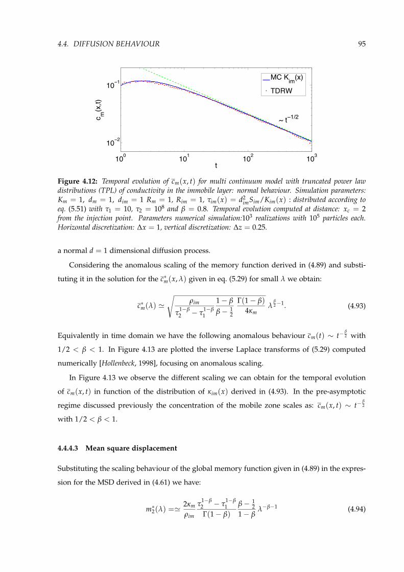
4.4. DIFFUSION BEHAVIOUR 95
100 101 102 103
10 2
10 1
t
c m(x
,t)
MC Kim(x)
TDRW
~ t 1/2
Figure 4.12: Temporal evolution of cm(x, t) for multi continuum model with truncated power lawdistributions (TPL) of conductivity in the immobile layer: normal behaviour. Simulation parameters:Km = 1, dm = 1, dim = 1 Rm = 1, Rim = 1, τim(x) = d2
imSim/Kim(x) : distributed according toeq. (5.51) with τ1 = 10, τ2 = 108 and β = 0.8. Temporal evolution computed at distance: xc = 2from the injection point. Parameters numerical simulation:103 realizations with 105 particles each.Horizontal discretization: ∆x = 1, vertical discretization: ∆z = 0.25.
a normal d = 1 dimensional diffusion process.
Considering the anomalous scaling of the memory function derived in (4.89) and substi-
tuting it in the solution for the c∗m(x, λ) given in eq. (5.29) for small λ we obtain:
c∗m(λ)
ρim
τ1−β2 − τ
1−β1
1− β
β− 12
Γ(1− β)4κm
λβ2−1. (4.93)
Equivalently in time domain we have the following anomalous behaviour cm(t) ∼ t−β2 with
1/2 < β < 1. In Figure 4.13 are plotted the inverse Laplace transforms of (5.29) computed
numerically [Hollenbeck, 1998], focusing on anomalous scaling.
In Figure 4.13 we observe the different scaling we can obtain for the temporal evolution
of cm(x, t) in function of the distribution of κim(x) derived in (4.93). In the pre-asymptotic
regime discussed previously the concentration of the mobile zone scales as: cm(x, t) ∼ t−β2
with 1/2 < β < 1.
4.4.4.3 Mean square displacement
Substituting the scaling behaviour of the global memory function given in (4.89) in the expres-
sion for the MSD derived in (4.61) we have:
m∗2(λ) = 2κm
ρim
τ1−β2 − τ
1−β1
Γ(1− β)β− 1
21− β
λ−β−1 (4.94)

96 CHAPTER 4. ANOMALOUS DIFFUSION IN COMPOSITE MEDIA
100 101 102 103 10410 3
10 2
10 1
100
t
c m(x
,t)
: 0.6: 0.7: 0.8: 0.9
~ t 0.3
~ t 0.4
~ t 0.35
~ t 0.45
Figure 4.13: Temporal evolution of cm(x, t) given in (5.29) for the multi continuum model consid-ering a truncated power law distribution of conductivity in the immobile layer. Anomalous scaling:cm(x, t) ∼ t−
β2 with 1/2 < β < 1. Parameters: ρm = 10−4, ρim = 1, χm = 0.02, χim = 10,
κm = 40, τim(x) = χ2imρim/κim(x): distributed according to the truncated power law distribution
given in (5.51) with τ2 = 250, τ2 = 107 and β indicated in the figure from 0.6 to 0.9, distanceobservation point from the injection point x = 2.
and considering its inverse Laplace transform we have the following scaling in time domain:
m2(t) tβ. In Figure 4.14 we plot the MSD for the multi continuum model given in (4.61)
for different truncated distributions of κim(x). Figure 4.14 shows the sub-diffusive anomalous
scaling derived analytically.
100 101 102 103 10410 2
100
102
104
t
MSD
TPL, :0.9TPL, :0.8TPL, :0.7TPL, :0.6
~ t
Figure 4.14: Mean squared displacement given in (4.61) for the multi continuum model, consideringa truncated power law distribution of conductivity in the immobile layer. Parameters: ρm = 0.0001,ρim = 1, χm = 0.02, χim = 10, κm = 40, τim: distributed according to the truncated power law givenin (5.51) with τ1 = 250, τ2 = 107 and β indicated in the figure from 0.6 to 0.9.

4.4. DIFFUSION BEHAVIOUR 97
4.4.4.4 First passage time distribution
Anomalous FPTD is obtained substituting (4.89) into the definition of the FPTD derived in
(4.65):
f ∗(λ) 12
e−
ρimκm
Γ(1−β)
τ1−β2 −τ
1−β1
1−β
β− 12
λβ2 |x|
. (4.95)
The previous equation corresponds to a Levy stable distribution. Expanding (4.95) for small
λ and using the Tauberian theorem to compute the inverse Laplace transform, we obtain the
follow anomalous scaling for the FPTD: f (t) ∼ t−β2−1, with 1/2 < β < 1 (see Appendix
C.4). As seen previously, asymptotically, the Laplace transform of memory function tends to
a constant value. Considering the inverse Laplace transform of (4.65) with ϕ∗(λ) ρim we
obtain that asymptotically the FPTD scales as f (t) ∼ t−3/2, as in an equivalent homogeneous
medium. In Figure 4.15 we plot the FPTD for the multi continuum model given in (4.65) for
different exponents of the truncated power law distribution of bulk conductivity. We observe
the anomalous scaling of the FPTD derived analytically.
100 101 102 103 104
10 6
10 3
100
t
FPTD
TPL :0.9TPL :0.8TPL :0.7TPL :0.6
~ t 1.3~ t 1.35
~ t 1.4~ t 1.45
Figure 4.15: FPTD for the multi continuum model given in (4.65) considering a truncated power lawdistribution of bulk conductivity. Parameters: ρm = 10−4, ρim = 1, χm = 0.02, χim = 10, κm = 40,x = 2, τim: distributed according to the truncated power law given in (5.51) with τ1 = 250, τ2 = 107
and β indicated in the figure from 0.6 to 0.9.
Anomalous scaling for the temporal evolution, MSD and FPTD of cm(x, t) are summed
concisely in Table 4.1.

98 CHAPTER 4. ANOMALOUS DIFFUSION IN COMPOSITE MEDIA
4.5 Conclusions
Anomalous diffusion has been observed largely observed in heterogeneous media and media
heterogeneity gives rise to a distribution of time scales. On this basis, we derived a multi
continuum model characterized by distribution of characteristic times.
The multi continuum models derived lead to anomalous behaviour in diffusion problems
of a scalar quantity cm(x, t). The models link anomalous scaling to a statistical description of
media heterogeneity. The dual continuum model derived shows pre-asymptotic anomalous
scaling, until a characteristic time given by the mean diffusion time in the immobile zone. Un-
like the earlier double porosity/permeability models [Barenblatt et al., 1960; Warren and Root,
1963; Dykhuizen, 1987; Peters and Klavetter, 1988; Dykhuizen, 1990; Bai et al., 1993]), which con-
sider quasi-equilibrium in each zone and first order mass transfer between the mobile and
the immobile regions, we considered non-equilibrium in the immobile zone which origins
anomalous behaviour. In the pre-asymptotic regime a sub-diffusive behaviour leads the MSD
of cm(x, t) scaling as t1/2, its FPTD as t−5/4 and its temporal evolution as t−1/4. Asymptoti-
cally diffusion becomes normal: MSD increases linearly in time, FPTD decreases as t−3/2 and
temporal evolution as t−1/2. In order to have sub-diffusion the bulk retardation coefficient (or
total storativity in the case of flow problem) of the mobile region must be far smaller that the
one of the immobile region. This condition is typically satisfied in fractured media, where
anomalous behaviour is observed. Increasing the heterogeneity of the model, a distribution of
diffusion parameters in the immobile layer leads to a larger range of anomalous sub-diffusive
behaviours. Considering a distribution of conductivity we obtain pre-asymptotic anomalous
behaviour, where MSD of cm(x, t) scales as tβ, FPTD as t−β/2−1 and temporal evolution as
t−β/2, with 0.5 < β < 1. Asymptotically diffusion became normal. Differently a distribu-
tion of retardation coefficients, or storativities considering a flow problem, can model the
same anomalous scaling also asymptotically and not only pre-asymptotically. The results ob-
tained are in accord with the theoretical work of Bouchaud on diffusion in disordered media
[Bouchaud and Georges, 1990]. Bouchaud demonstrated that a barrier model, equivalent to a
variable conductivity model can not lead to an asymptotic anomalous behaviour, while a trap
model, that can be mapped into a variable storativity model, can lead to anomalous asymp-
totic sub-diffusive behaviour. In this work we link the anomalous behavior in diffusion process
to media heterogeneity. Spatial distribution of hydraulic parameters implies in diffusion prob-
lem a distribution of timescales. We link the spatial distribution of diffusion parameters to

4.5. CONCLUSIONS 99
a distribution of timescales and we link the anomalous behaviour to particular distribution
of timescales. We point out that the same time scale distribution in a medium characterized
by variable conductivity and variable retardation coefficient induces different asymptotic be-
haviours. This indicates that the dynamic of a medium characterized by spatially variable
conductivity and spatially variable retardation factor is intrinsically different.

100 CHAPTER 4. ANOMALOUS DIFFUSION IN COMPOSITE MEDIA

Chapter 5
Catchment Response in Frequency
Domain
I
Anomalous temporal scaling of catchment responses in discharge and groundwater levels
observed in hydrological systems are commonly explained by fractal models, which, however,
often lack a relation to the medium characteristics and are rather descriptive. Here we employ
a multi-continuum approach to model such anomalous behavior. This approach is based on
a stochastic model description of the medium heterogeneity, and thus, in principle, allows
to relate the catchment response to the distribution of hydraulic parameters. The temporal
scaling of groundwater levels and discharge is quantified in frequency domain by the transfer
function Θ(ω), which is defined as the ratio between the spectra of catchment response and
recharge. The transfer function may scale with frequency ω as Θ(ω) ∼ ω−β. While the
classical linear and Dupuit models predict exponents of β = 2 and β = 1, respectively, the
proposed multi-continuum models can explain exponents 1/2 < β < 2. Moreover we revise
and integrate the classical linear first-order and Dupuit models in the light of the aquifer
dynamics, showing that the scaling exponent of the related transfer functions depends on
the boundary condition chosen at the discharge boundary. We systematically analyze the
catchment response in the proposed multicontinuum models, and identify and quantify the
time scales which characterize the dynamics of the catchment response to recharge.
IThis chapter is part of a paper Temporal Scaling of Groundwater Levels and Discharge in Dual and Multi-ContinuumCatchment Models, Russian A., M. Dentz, T. Le Borgne, J. Carrera and J. Jimenez-Martinez; to be submitted toWater Resources Research. Part of the work in this chapter have contributed to the paper: A frequency domainanalysis to characterize heterogeneity and recharge mechanisms in a fractured crystalline-rock aquifer Jiménez-Martínez J.,L. Longuevergne, T. Le Borgne, P. Davy, A. Russian, O. Bour; under review in Water Resources Research.
101

102 CHAPTER 5. CATCHMENT RESPONSE IN FREQUENCY DOMAIN
5.1 Introduction
The understanding of the relation between aquifer discharge and recharge is a fundamental
problem in hydrology. Often, aquifer discharge into a river or any outfall is the only infor-
mation available when studying the groundwater system of a basin. This information may be
enough to model regional flow, disregarding the details at local scales [Duffy and Lee, 1992].
The discharge of a catchment is a measure for the recharge at basin-scale, and variations in the
discharge represent the dynamic response of an aquifer to changes in recharge. A clear un-
derstanding of the ground water system dynamics and the recharge processes is fundamental
to improve our ability to manage groundwater resources.
Modeling aquifer recharge is a challenging problem due to the variety of physical pro-
cesses involved and the limited information available on hydraulic parameters, aquifer prop-
erties and geometry [Scanlon et al., 2002]. Because of the scarcity of information and the
intrinsic complexity in the recharge process, it is useful to keep the models of aquifer recharge
simple and linked to a stochastic medium description.
One of the main characteristics in aquifer recharge is the temporal variability in the
recharge process. Rainfall enters the aquifer system in an irregular way, but the hydrograph
related to the discharge, q(t), or to the groundwater lever h(x, t), are characterized by a cer-
tain periodicity [e.g., Gelhar and Wilson, 1974; Besbes and De Marsily, 1984; Duffy and Cusumano,
1998; Manga, 1999]. The simplest way to describe this behavior is to consider the catchment
as a linear input-output system, where the input (rainfall) and the output (groundwater head
variation or the consequent discharge) are related linearly through a transfer function. The
transfer function quantifies the action of the aquifer on the discharge dynamics. In this context,
the aquifer is considered a linear filter whose properties depend on the medium characteris-
tics and flow processes in the medium [e.g., Gelhar, 1974; Freeze, 1975; Duffy and Gelhar, 1985;
Juki and Denijuki, 2004; Zhang, 2004]. Spectral analysis provides a useful tool to characterize
the input and output signals and analyze the filter properties of the aquifer [e.g., Gelhar, 1974].
In this framework, the aquifer dynamics are quantified by the power spectrum of the transfer
function, which in the following is termed the frequency transfer function Θ(ω).
Classical aquifer models to determine the transfer function are the linear reservoir (LR)
model and the linear Dupuit (LD) aquifer model [e.g., Gelhar, 1974]. The LR model is 0–
dimensional and thus disregards spatial variations of hydraulic head. The LD model is 1–
dimensional and describes flow in the aquifer based on the linearized Dupuit-Forchheimer

5.1. INTRODUCTION 103
hypothesis [e.g., Bear, 1972]. These models are illustrated schematically in Figure 5.1. They
predict that for high frequencies ω, the transfer function related to the discharge flux scales
as Θ(ω) ∼ ω−β. The LR model predicts a scaling exponent of β = 2 [Gelhar, 1974], the LD
model a scaling exponent of β = 1 [Gelhar, 1974; Molenat et al., 1999]. The difference in the
scaling exponents implies a difference in the aquifer response dynamics.
Scaling behaviors with exponents β = 1, 2 are called ’anomalous’. A series of studies
have shown that groundwater levels and discharge signals [e.g., Zhang and Yang, 2010; Labat
et al., 2002; Zhang, 2004; Molenat et al., 1999, 2000; Jiménez-Martínez et al., 2012] as well as
river runoff [e.g., Tessier et al., 1996; Kantelhardt et al., 2003; Zhang, 2005; Kantelhardt et al., 2006;
Koscielny-Bunde et al., 2006; Livina et al., 2007; Little and Bloomfield, 2010] may scale anomalously.
Such behavior cannot be explained by classical recharge models, which are based on the
representation of the aquifer as a homogeneous porous medium. Geological media are in
general heterogeneous and thus the flow dynamics are more complex than in homogeneous
media. Specifically, spatial heterogeneity induces a spectrum of transfer time scales, which
the classical models are not able to describe. For example, after a recharge event, a portion
of water may flow quickly to the discharge point according to the piezometric head gradient,
whereas another portion may infiltrate in low permeability regions and get stored there to
be released slowly at a later time. As indicated by Hurst [1951], long-range correlations in
river responses indicate that water storage and discharge processes occur over a wide range
of temporal scales [Tessier et al., 1996; Fiori et al., 2009; Duffy, 2010].
Anomalous scaling of the frequency transfer function is typically modeled using multi-
fractal approaches [e.g., Turcotte and Greene, 1993; Tessier et al., 1996; Kantelhardt et al., 2003;
Labat et al., 2011]. A limitation of these models is that the fractal dimension is not directly
linked to the spatial organization of the aquifer, and it can vary depending on the experi-
mental conditions used to determine it [e.g., Little and Bloomfield, 2010]. For these reasons, the
interpretation of multi-fractal models is rather difficult [Tessier et al., 1996], which limits their
usefulness for prediction [Labat et al., 2002]. Zhang [2004] pointed out that anomalous scaling
in the aquifer response may be due to medium heterogeneity, or fractality of the recharge
process, or a combination of both.
In this paper we focus on the role of medium heterogeneity for the anomalous scaling of
the aquifer response to recharge. The objective is to establish a physical model that renders a
wide range of water storage scales, that is able to explain anomalous behavior and that allows
to link the anomalous dynamics of the discharge process to the distribution of storage scales

104 CHAPTER 5. CATCHMENT RESPONSE IN FREQUENCY DOMAIN
as reflected in the physical aquifer characteristics. To this end, we consider dual and a multi-
continuum aquifer models that can explain pre-asymptotic anomalous scaling of the transfer
function due to the medium heterogeneity. Early double porosity and double permeabil-
ity models assume that the mobile and the immobile zones are each in quasi-equilibrium and
therefore mass transfer is approximated as a first order process [e.g. Barenblatt et al., 1960; War-
ren and Root, 1963; Dykhuizen, 1987, 1990]. Our approach takes into account non-equilibrium
effects in the immobile zone, which gives rise to anomalous behaviour. In the following, we
revisit and extend the classical recharge models and discuss their physical meanings in the
light of the resulting aquifer dynamics. On the basis of these classical model, we dervie dual
and multi-continuum recharge models which are able to explain anomalous scaling of the
frequency transfer function and link this behavior to a statistical description of the medium
heterogeneity.
In the following we consider two classical models: the linear reservoir (LR) model and
the linear Dupuit (LD) model with different boundary conditions at the discharge point. In
modeling recharge dynamics as an input-output problem, linearity implies that the output
signal (the groundwater level or the consequent discharge) represents a unique response to a
given input (recharge). It is assumed that the recharge r(t) is spatially uniform. Considering
ground water discharge q(t) as output, it can be written as a linear functional of the input
signal r(t),
q(t) =∞
−∞
fq(τ) r(t− τ)dτ, (5.1)
where fq(τ) is the discharge impulse response function, or filter, of the system [Wiener, 1949].
This convolution on the right side transforms to a product in frequency domain. The Fourier
transform here is defined by
F(ω) =∞
−∞
f (t) exp(−iωt)dt, f (t) =∞
−∞
F(ω) exp(iωt)dω
2π(5.2)
with i the imaginary unit. Taking the Fourier transform of (5.1) and solving for the Fourier
transform of fq(t), we obtain the complex frequency discharge response function Fq(ω) as the

5.1. INTRODUCTION 105
ratio of the Fourier transform of the discharge Q(ω) and the recharge R(ω),
Fq(ω) =Q(ω)R(ω)
. (5.3)
Its square is the frequency transfer function (FTF) [Box and Jenkins, 1970]:
Θq(ω) = |Fq(ω)|2. (5.4)
The discharge FTF Θq(ω) characterizes the dynamics of the catchment at basin scale and
allows to model recharge dynamics to predict the aquifer response to various hydrological
scenarios.
5.1.1 Linear Reservoir Model
In the LR model an aquifer is considered as a lumped linear reservoir system. It is a 0-
dimensional model, where spatial variation of water levels are neglected and the average
thickness of the saturated zone h(t) is a function of time only [Gelhar, 1974; Bear, 1972]. A
schematic illustration of the model is given in Figure 5.1. The governing equation of the LR
model is
Sdh(t)
dt= −q(t) + r(t), q(t) = a[h(t)− h0], (5.5)
where S is the storage coefficient [−], q(t) is the outgoing flux per unit area of aquifer surface
[LT−1], a is an outflow constant [T−1], h0 is the reference level of the adjacent outfall body of
water, and r(t) is recharge [LT−1] per unit area of the aquifer. For simplicity in the following
we set the reference level h0 to zero without loss of generality. The discharge FTF for the LR
model is:
Θq(ω) =1
1 + (tω)2 , (5.6)
where t is a characteristic response time given by t = S/a [Gelhar and Wilson, 1974]. Frequen-
cies lower than t−1 are not damped by the system, while for higher frequencies the transfer
function scales as Θq(ω) ∼ ω−2.
In addition to the groundwater discharge q(t), we consider also the groundwater level h(t)

106 CHAPTER 5. CATCHMENT RESPONSE IN FREQUENCY DOMAIN
Figure 5.1: Conceptual illustration of the classical recharge models. From left: LR model, LD modelwith Dirichlet BC, Dupuit model with Cauchy BC. In the figures: q(t) stream discharge, r(t) aquiferrecharge, considered uniform, h(x, t) or h(t) hydraulic head, L length of the catchment, h0 head level ofthe outfall basin. h0 indicates the imposed fixed head at the BC of the LD model with Dirichlet BC. Inthe LR model and in the LD model with Cauchy BC q(t) indicates the imposed flux BC. In the Dupuitmodels at x = L no-flux BC at the watershed is imposed.
as output signal in the input-output catchment model. The head FTF, Θh(ω), is given by:
Θh(ω) =
H(ω)R(ω)
2
. (5.7)
In the LR model the groundwater head and discharge flux are related by the outflow constant
a as given in (5.5). Setting the reference level h0 to 0, the head FTF Θh(ω) is related to the
discharge FTF as: Θq(ω) = a2Θh(ω). Consequently, the head FTF for the LR model reads:
Θh(ω) =1
a + (ωS)2 . (5.8)
Notice that the scaling for large frequencies for both the groundwater discharge and the
ground water level is the same Θh(ω) ∼ Θq(ω) ∼ ω−2.

5.1. INTRODUCTION 107
5.1.2 Linear Dupuit Model
The LD model is based on the linearized form of the Dupuit approximation [Bear, 1972], which
is given by [Gelhar, 1974]
S∂h(x, t)
∂t− T
∂2h(x, t)∂x2 = r(t), (5.9)
where S is storativity, h(x, t) hydraulic head, T transmissivity and r(t) recharge per unit area
of the aquifer. The head frequency transfer function is defined as above as
Θh(x, ω) =
H(x, ω)R(ω)
2
. (5.10)
It is obtained from the solution of the temporal Fourier transform of (5.9),
iωSH(x, ω)− T∂2H(x, ω)
∂x2 = R(ω) + S h(x, 0). (5.11)
In order to compare the discharge flux with the recharge, it is convenient to consider the
discharge per unit area of the surface of the aquifer. Per Darcy’s law, the discharge per unit
area in Fourier space, Q(ω), is given by,
Q(ω) =TL
∂H(x, ω)∂x
x=0
. (5.12)
As illustrated in Figure 5.1, the Dupuit model represents an homogeneous catchment with
a no flow boundary condition (BC) at the watershed (Neumann BC) [∂h(x, t)/∂x]x=L = 0. At
the discharge boundary typically prescribed head (Dirichlet BC) is assumed [e.g. Gelhar, 1974;
Molenat et al., 1999]. However, Dirichlet discharge boundary conditions may not always be
realistic and in many situation Cauchy BCs may be more appropriate [e.g., Bear, 1972]. In
the following we discuss the behaviour of the FTF depending on the choice of the discharge
boundary conditions.
5.1.2.1 Dirichlet Boundary Condition
The Dirichlet BC prescribes the head at the discharge boundary at x = 0, h(x = 0, t) = t) = h0.
Without loss of generality we set h0 = 0 in the following. Furthermore, we refer to the LD
model with Dirichlet boundary conditions as LDD model in the following. With this BC, the

108 CHAPTER 5. CATCHMENT RESPONSE IN FREQUENCY DOMAIN
solution of (5.11) is given by
H(x, ω) =R(ω)iωS
1−
coshp(ω)
xL − 1
cosh [p(ω)]
, (5.13)
see also [Gelhar, 1974]. We defined here
p(ω) =
iωtL, tL = L2S/T. (5.14)
The characteristic response time tL represents the mean diffusion time over the length of the
aquifer. The importance of the aquifer response rate given by t−1L is discussed in Erskine and
Papaioannou [1997]. Using (5.13) in (5.12) and the definition of the discharge response function
(5.2) we obtain the following expression for the discharge FTF,
Θq(ω) =1
ωtL|tanh[p(ω)]|2 . (5.15)
The head FTF defined by (5.10) can be directly read of expression (5.13) and is given by
Θh(x, ω) =1
ω2S2
1−cosh
p(ω)
xL − 1
cosh [p(ω)]
2
. (5.16)
Notice that Θh(x, ω) and Θq(ω) are characterized by different scalings unlike in the LR model.
For high frequencies, Θq(ω) scales as ω−1. The scaling of Θh(x, ω) depends on the observation
point x. Close to the discharge point at x = 0, it scales as ω−1, that is, like the discharge FTF.
For an observation point near the watershed at x = L and ω t−1L it scales as ω−2, which
is the scaling behavior of the LR model at high frequencies. The behaviors of Θq(ω) and
Θh(x, ω) are illustrated in Figures 5.2 and 5.3, respectively.
5.1.2.2 Cauchy Boundary Condition
The Cauchy boundary condition relates the discharge flux with the difference of the boundary
head and a reference head h0 in the outfall as
TL
∂h(x, t)∂x
x=0
= a [h(0, t)− h0], (5.17)
where a is an outflow constant. Without loss of generality the reference level is set to zero
h0 = 0. Furthermore, we refer to the LD model with Cauchy Boundary conditions as LDC in

5.1. INTRODUCTION 109
the following. With this BC the solution of (5.11) is given by
H(x, ω) =R(ω)iωS
1−
coshp(ω)
xL − 1
p(ω)TaL2 sinh[p(ω)] + cosh[p(ω)]
, (5.18)
with p(ω) given by (5.14). Notice that for p(ω)T/L2 a, (5.18) reduces to (5.13). This implies
that in the time regime t (ST)/(aL)2 the dynamics of the LDD and LDC models are the
same. Using (5.18) in (5.12), the discharge frequency transfer function Θq(ω) is
Θq(ω) =a2
ω2S2
tanh[p(ω)]
tanh[p(ω)] + aL2
p(ω)T
2
. (5.19)
That head FTF again can be directly read of from (5.18) according to (5.10) and is given by
Θh(ω) =1
ω2S2
1−cosh
p(ω)
xL − 1
p(ω)TaL2 sinh[p(ω)] + cosh[p(ω)]
2
, (5.20)
Notice that for large ω, the head FTF Θh(x, ω) ∼ a−1Θq(ω) ∝ ω−2. Both transfer functions
scale as ω−2. The behavior of the head FTF is at large frequencies independent from the
observation point x, as in the LR model. In fact, in the Appendix D.1 we show that the LR
model can be obtained from the horizontal average of the LDC model.
5.1.3 Discussion
Here we briefly discuss the dynamics of the models presented above focusing on the scaling
of the corresponding transfer functions illustrated in Figures 5.2 and 5.3). The discharge FTF
Θq(ω) for the models considered above are shown in Figure 5.2. The dynamics of Θq(ω)
is controlled by a single characteristic frequency ωL, the aquifer response rate [Erskine and
Papaioannou, 1997]. The aquifer response rate is given by ωL = t−1L = T/(L2S) for the LD
models and by ωL = t−1 = a/S for the LR model. For frequencies lower than ωL, Θq(ω) is
equal to one for all the models considered, while for larger frequencies it decreases and scales
according to the related recharge model. For the LDD model, the FTF scales as Θq ∼ ω−1,
and for the LR and LDC models as Θq ∼ ω−2. This means that long time components in the
recharge spectrum, with frequencies lower than the aquifer response rate are not smoothed by
the system and their variations reflect unaltered on the output. Higher frequency components
of the recharge spectra are smoothed according to the model considered. Moreover, Figure 5.2

110 CHAPTER 5. CATCHMENT RESPONSE IN FREQUENCY DOMAIN
shows that the LDC model slightly differs from the LR model only in an intermediate fre-
quency regime, while for ω t−1L and ω t−1
L the two models coincide. For this reason, in
the following, we disregard the first order linear model, and focus on the two LD models.
It is also interesting to note, that Gelhar [1974] derived the outflow constant a, which is
characteristic of the LR model, from the LDD model and obtained a = L2/(3T). In Ap-
pendix D.1 we show that the LR model in fact corresponds to the LDC model. As outlined
above, the behaviors of the LDC and LDD models are different. Thus, we conclude that the
derivation of the outflow constant a from the LDD is rather inconsistent. Alternatively, we
propose to determine a by comparing the response time of the LR model, which is t = S/a,
and the response time of the LD models tL = L2S/T. This leads to a = L2/T.
10 2 10 1 100 101 102 10310 6
10 4
10 2
100
q ()
DupuitLinearCauchy
2
1
L = T/(SL2)
Figure 5.2: FTF for discharge Θq(ω). Shown are the (triangles) LDD model, (squares) LDC model(solid line) LR model. The vertical dotted line indicates the aquifer response rate ωL which is ωL =t−1
L = T/(L2S) for the LD model and ωL = t−1 = a/S for the LR model. The parameters used are
S = 1, T = 1, L = 1.
Figure 5.3 displays Θh(x, ω) for the LDD and LDC models for different observation points:
x = L, x = L/20 and x = L/100. All the Θh(x, ω) are constant until the aquifer response rate
ωL discussed above, and then decrease according to respective model behavior. Considering
the LDC model, the scaling of Θh(x, ω) does not depend on the observation point in the
aquifer and it scales as Θh(x, ω) ∼ ω−2 analogously to Θq(x, ω) displayed in Figure 5.2.
For the LDD model, in contrast, the scaling of Θh(x, ω) depends on x. The spatial de-
pendency of Θh(x, ω) in the LDD model introduces a second characteristic time tx = Sx2/T,
which is given by the mean diffusion time from the observation point to the discharge point.
Depending on the observation point x, the head FTF Θh(x, ω) scales as ω−1 until ωx = t−1x
and for ω ωx, it scales as ω−2 as in the LDC and LR models. The scaling ω−1 is observed
if we have scale separation between the aquifer response time tL = L2S/T and tx. Close to
the discharge point, the transfer function for the ground water level Θh(x, ω) scales similarly
to Θq(ω). Indeed, the discharge flux is given by Darcy’s law and near the discharge point, for

5.2. MULTI-CONTINUUM RECHARGE MODELS 111
x → 0, we can approximate
∂h(x, t)∂x
x=0
h(x, t)x
. (5.21)
Note that we set h(x = 0, t) = 0. Thus, Θq(ω) and Θh(x, ω) scale the same way close to the
discharge point. Close to the watershed Θh(L, ω) ∼ ω−2 behaves as for the LR because the
system resembles a linear reservoir.
Furthermore, we observe that the value of the head FTF at ω = 0 depends on the respective
LD model. Taking the limit ω → 0 in Θh(x, ω), (5.13), for the LDD model gives
limω→0
Θh(x, ω) =−
x2
2T+
LxT
2
(5.22)
For the LDC model we obtain from taking ω → 0 in (5.18),
limω→0
Θh(x, ω) =−
x2
2T+
LxT
+1a
2
. (5.23)
For large values of a, the FTFs of the LDD and LDC models coincide. In general they are
different, however. The values of both FTF decrease at ω = 0 as the observation point gets
closer to the discharge boundary.
100 102 10410 10
100
h ()
Cau x=LCau x=L/20Cau x=L/102
Dup x=LDup x=L/20Dup x=L/102
1
x = T/(Sx2)
2
Figure 5.3: Head FTF Θh(ω) for different observation points for the LDD and LDC models. Thevertical dotted lines indicate the characteristic frequencies ωx = t−1
x = T/(x2S) for the differentobservation points at x = L, L/20 and L/102. The parameters used are S = 1, T = 1, L = 1.
5.2 Multi-Continuum Recharge Models
In this section we present multi-continuum recharge models which account for the impact of
regions of different hydraulic properties in the aquifer. The models derived assume that the
water entering the aquifer infiltrates into a conductive region through which it may flow to

112 CHAPTER 5. CATCHMENT RESPONSE IN FREQUENCY DOMAIN
the discharge point according to the hydraulic gradient, and from which it may infiltrate into
less conductive zones, where it can get trapped and again slowly released. For simplicity,
the conductive zone is called mobile region, while the less conductive one is called immobile
region. The wide range of temporal scales which characterize natural problems [Tessier et al.,
1996; Fiori et al., 2009; Duffy, 2010], can arise here from an heterogeneous immobile layer,
which statistically described by a distribution of hydraulic parameters. For completeness we
take into account also the case of an homogeneous immobile layer, which reduces the multi-
continuum recharge model to a dual-continuum recharge model. The underlying conceptual
models are illustrated schematically in Figure 5.4.
5.2.1 Model Derivation
The governing equation of the multi-continuum recharge model is given by the flow equation
s(x)∂h(x, t)
∂t−∇ · [K(x)∇h(x, t)] = 0, (5.24)
where x = (x, z)T. In the immobile region, 0 < z < dim, specific storativity and hydraulic
conductivity are variable in x–direction, s(x) = sim(x) and K(x) = Kim(x), while in the mobile
region, dim < z < d, both specific storativity and hydraulic conductivity are constant, s(x) =
sm and K(x) = Km. The system is driven by the recharge r(t) at the upper horizontal boundary
of the mobile layer, which yields the boundary condition
Km∂h(x, t)
∂z= r(t), z = d. (5.25)
At the lower boundary a no flux boundary condition is specified
Kim(x)∂h(x, t)
∂z= 0, z = 0. (5.26)
As initial condition we set h(x, 0) = 0. The hydraulic heads in the mobile and immobile
regions are denoted by him(x, t) = h(x, t) for 0 < z < dim, and hm(x, t) = h(x, t) for dim < z < d.
Both head and flux are continuous at the interface between the two mobile and immobile
regions
hm(x, t) = him(x, t), Km∂hm(x, t)
∂z= Kim(x)
∂him(x, t)∂z
, z = dim. (5.27)

5.2. MULTI-CONTINUUM RECHARGE MODELS 113
5.2.1.1 Vertical Average
In order to arrive at an effective description, we average the flow equation (5.24) vertically.
The average hydraulic heads in the mobile and immobile regions are defined as
Figure 5.4: On the left: dual-continuum model, on the right: multi-continuum model. The catchmentof longitude L and thickness d = dm + dim is split into a superficial layer of thickness dm, whichrepresents the mobile layer and a lower less permeable layer, of thickness dim, which is the immobilelayer; q(t) is the stream discharge, r(t) the aquifer recharge and hm(x, t) and him(x, t) the hydraulicheads in the mobile and in the immobile zones, respectively.
him(x, t) =1
dim
dim
0
dz him(x, t), hm(x, t) =1
dm
d
dim
dz hm(x, t) (5.28)
By averaging of (5.24) over the mobile region, we obtain for hm(x, t) the governing equation
Sm∂hm(x, t)
∂t− Tm
∂2hm(x, t)∂x2 = r(t)− Kim(x)
∂him(x, t)∂z
z=dim
, (5.29)
where we used the continuity condition (5.27) and defined the storage capacity Sm = smdm
and transmissivity Tm = Kmdm of the mobile region, as well as recharge r(t) = dmr(t). The
last term in (5.29) represents the flux at the interface between mobile and immobile regions
and it is obtained from the solution of the flow equation in the immobile domain, which is
given by
sim(x)∂him(x, t)
∂t− Kim(x)
∂2him(x, t)∂z2 = 0, (5.30)
Notice that we have disregarded flow in horizontal direction in the immobile layer because it
is small compared to the one in the more conductive region. Furthermore, we assume that
vertical equilibrium in the mobile layer is reached fast so that we can set hm(x, t) ≈ hm(x, t).
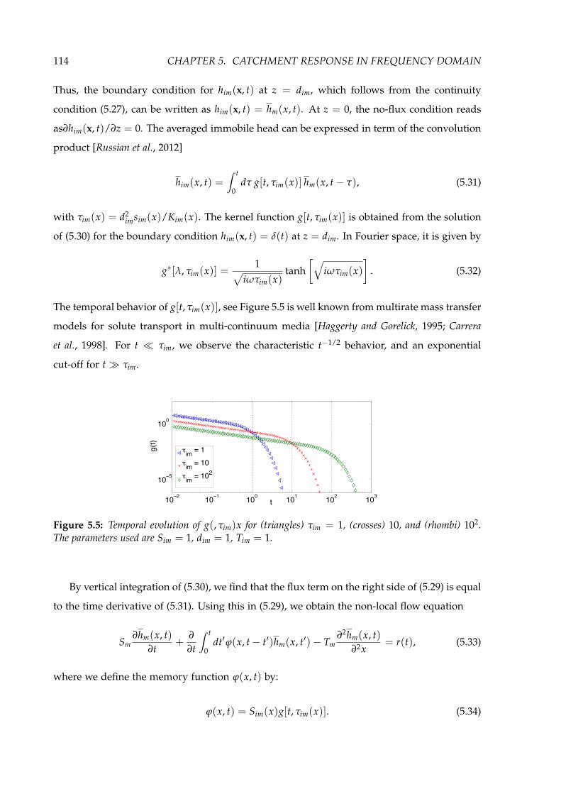
114 CHAPTER 5. CATCHMENT RESPONSE IN FREQUENCY DOMAIN
Thus, the boundary condition for him(x, t) at z = dim, which follows from the continuity
condition (5.27), can be written as him(x, t) = hm(x, t). At z = 0, the no-flux condition reads
as∂him(x, t)/∂z = 0. The averaged immobile head can be expressed in term of the convolution
product [Russian et al., 2012]
him(x, t) = t
0dτ g[t, τim(x)] hm(x, t− τ), (5.31)
with τim(x) = d2imsim(x)/Kim(x). The kernel function g[t, τim(x)] is obtained from the solution
of (5.30) for the boundary condition him(x, t) = δ(t) at z = dim. In Fourier space, it is given by
g∗[λ, τim(x)] =1
iωτim(x)tanh
iωτim(x)
. (5.32)
The temporal behavior of g[t, τim(x)], see Figure 5.5 is well known from multirate mass transfer
models for solute transport in multi-continuum media [Haggerty and Gorelick, 1995; Carrera
et al., 1998]. For t τim, we observe the characteristic t−1/2 behavior, and an exponential
cut-off for t τim.
10 2 10 1 100 101 102 103
10 5
100
t
g(t)
im = 1
im = 10
im = 102
Figure 5.5: Temporal evolution of g(, τim)x for (triangles) τim = 1, (crosses) 10, and (rhombi) 102.The parameters used are Sim = 1, dim = 1, Tim = 1.
By vertical integration of (5.30), we find that the flux term on the right side of (5.29) is equal
to the time derivative of (5.31). Using this in (5.29), we obtain the non-local flow equation
Sm∂hm(x, t)
∂t+
∂
∂t
t
0dtϕ(x, t− t)hm(x, t)− Tm
∂2hm(x, t)∂2x
= r(t), (5.33)
where we define the memory function ϕ(x, t) by:
ϕ(x, t) = Sim(x)g[t, τim(x)]. (5.34)
5.2. MULTI-CONTINUUM RECHARGE MODELS 115
with Sim(x) = dimsim(x). Notice that Eq. (5.38) is analogous to the LD model given in (5.9),
but reflects the presence of different storage time scales in the medium, which gives rise to the
non-local term. The memory function represents the dynamics of the recharge and storage
process in the immobile layer. In this sense, (5.38) can be seen as a time non-local LD model.
5.2.1.2 Ensemble Average
We handle spatial heterogeneity of the immobile zone in a stochastic framework and spatially
varying hydraulic conductivity is modeled as spatial random fields. We consider a stationary
and ergodic medium, with a finite correlation. For an observation scale far larger than the cor-
relation scale of the random medium, we can approximate the medium organization in bins,
where conductivities in each bins are independent. Thus, such medium can be completely
defined by a single point distribution. Referring to Figure (5.4) heterogeneity of the immobile
layer is organized in bins and at each bin is assigned independently a random conductivity
from a distribution.
In order to obtain an upscaled effective formulation, we average the effective governing
equations (5.38) horizontally over the immobile zone. Ensemble average over the heterogene-
ity of the immobile zone of equations (4.24) gives:
Sm∂hm(x, t)
∂t+
∂
∂t
t
0
dtϕ(t− t|x) hm(x, t) = Tm∂2hm(x, t)
∂x2 + r(t) (5.35)
where the square brackets indicate ensemble average. Ensemble average in the second term
of eq. (5.35) can not be executed explicitly. Thus, we use field approximation and we break
the ensemble average:
ϕ(t− t|x) hm(x, t) ≈ ϕ(t|x) hm(x, t). (5.36)
We define a global memory function ϕ(t) given by the ensemble average of the local
memory functions ϕ(t|x) associated at each immobile zone:
ϕ(t) = ϕ(t|x). (5.37)
116 CHAPTER 5. CATCHMENT RESPONSE IN FREQUENCY DOMAIN
Thus, we obtain the following upscaled equation:
Sm∂hm(x, t)
∂t+
∂
∂t
t
0dtϕ(t− t)hm(x, t)− Tm
∂2hm(x, t)∂2x
= r(t), (5.38)
where, for brevity of notation, we omit the square brackets. In the following we also omit the
square brackets for brevity of notation.
5.2.1.3 Solutions
Notice that when the mobile and the immobile zone are vertically in equilibrium, as we dis-
cuss in the following, (5.38) reduces asymptotically to a local flow equation for an equivalent
homogeneous media
Sa∂hm(x, t)
∂t− Tm
∂2hm(x, t)∂2x
= r(t), (5.39)
with a total storativity given by: Sa = Sm + Sim where Sim indicate the ensemble average of
Sim(x) in the multi-continuum case and is equal to Sim in the dual-continuum case. Equation
(5.38) can be conveniently written in frequency domain as
iωSe(ω)Hm(x, ω)− Tm∂2Hm(x, ω)
∂2x= R(ω), (5.40)
where we defined an effective function Se(ω):
Se(ω) = Sm + ϕ(ω). (5.41)
In frequency domain, the governing equation of the multi-continuum recharge model (5.40)
is equal in form to the Fourier transform of the LD model given in (5.11), with Se(ω) instead
of S. Consequently, the expression for the frequency transfer functions for the recharge multi-
continuum models, can be obtain by substituting S by Se(Ω) in the respective expressions for
the LD models.
Dirichlet Boundary Condition Thus, solution of (5.40) results: The transfer function for the
multi-continuum model with Dirichlet BC related to the ground water level reads:
H(x, ω) =R(ω)
iωSe(ω)
1− cosh [pe(ω)(1− x)]
cosh[pe(ω)]
, (5.42)

5.2. MULTI-CONTINUUM RECHARGE MODELS 117
with pe(ω) =
iωτe(ω) and τe(ω) = L2Se(ω)/Tm and the discharge FTF:
Θq(ω) =
1iωτe(ω)
tanh[pe(ω)]2
. (5.43)
Cauchy Boundary Condition Considering Cauchy BC at the discharge, solution of (5.40) is:
H(x, ω) =R(ω)
iωSe(ω)
1− cosh [pe(ω)(1− x)]
pe(ω)TaL2 sinh[pe(ω)] + cosh[pe(ω)]
(5.44)
and discharge FTF is given by:
Θq(ω) =
aLiωSe(ω)
tanh[pe(ω)]
tanh[pe(ω)] + aL2
pe(ω)T
2
. (5.45)
5.2.2 Dual-Continuum Recharge Model
Considering an homogeneous immobile zone, the multi-continuum model reduces to a dual-
continuum one. The governing equation is given by (5.38) with sim and Kim instead of sim(x)
and Kim(x). Considering equation (5.32), where τim(x) = τim, the characteristic time τim
indicates the mean time for the immobile zone to reach equilibrium by diffusion along the
vertical direction. For times larger than τim, considering ω τ−1im , the memory function
(5.32) scales as g(ω) ∼ (ωτim)−1/2 and therefore also Se(ω) given in (5.41) can scales as
Se(ω) ∼ ω−1/2 if
Sim(ωτim)−1/2 Sm. (5.46)
The previous condition is satisfied for ω (Sim/Sm)2/τim, which identifies a characteristic
threshold frequency ωS or equivalently a characteristic time τS = ω−1S given by:
τS =
Sm
Sim
2τim =
d2im S2
mTim Sim
(5.47)
and anomalous scaling of Se(ω) is defined in the interval:
τ−1im ω τ−1
S . (5.48)
In order to interpret the characteristic time τS, when anomalous behaviour starts, we call ∆z
the characteristic penetration of water by diffusion into the immobile layer after the time τS:
∆z =√
TimτS/Sim and (5.46) can be re-written as: ∆z Sim dmSm which indicates that the

118 CHAPTER 5. CATCHMENT RESPONSE IN FREQUENCY DOMAIN
amount of water into the immobile layer must be larger than the amount of water into the
mobile one. For time smaller than τS, flow takes place basically only into the mobile layer and
the contribution of the immobile one is negligible. After the time τS enough water infiltrated
into the immobile zone and its contribution is relevant.
In the following we focus on the anomalous scaling of the transfer functions for the dual-
continuum model considering the anomalous scaling of Se(ω) in the pre-asymptotic regime
defined in (5.48).
5.2.2.1 Dirichlet Boundary Condition
Considering the double continuum model with Dirichlet BC, the transfer function given in
(5.43) scales anomalously as:
Θq(ω) Tm
SimL2
ω
τim
−1/2(5.49)
instead of the Θq(ω) ∼ ω−1 as in the classical local LD model with Dirichlet BC. For ω larger
than τ−1S , Θq(ω) tends to the classical scaling Θq(ω) ∼ ω−1. The behaviour of the Θq(ω)
is shown in Figure 5.6. For large ω, which corresponds to short times the flow takes place
essentially only in the more conductive zone and Θq(ω) behaves as in a homogeneous media
characterized by the parameters of the mobile zone. After a time τS enough water has entered
the immobile zone, its contribution is relevant and we can observe anomalous scaling until
time τim, when also the immobile zone is in equilibrium along the vertical direction and the
system behaves as an equivalent homogeneous media and follows the classical behaviour of
the LD model.
The scaling of the head FTF Θh(ω), as discussed previously in Section 5.1.2.1, depends on
the observation point x in the aquifer. Near the watershed, for x to L, instead of the classical
scaling ω−2, in the pre-asymptotic regime given in (5.48), we obtain Θh(ω) ∼ ω−1. At the
discharge point, for x to 0, instead of ω−1 we have Θh(ω) ∼ ω−1/2. For this reason in the
following we point out only the scaling of Θq(ω) which is characteristic of the model and
does not depend on the observation point.

5.2. MULTI-CONTINUUM RECHARGE MODELS 119
100 105 1010
10 5
100
q ()
tm11
imte1
~ 0.5
1S
Figure 5.6: Frequency transfer function for ground water discharge for the dual-continuum modelwith Dirichlet BC (triangles). Dots: Θq(ω) considering only the mobile layer; crosses: Θq(ω) forhomogeneous equivalent model with effective storativity given by (5.2.1.3). Anomalous scaling ω−0.5
is indicated with the continuous line. Vertical dashed lines mark the characteristic times (given on theleft side) that control the dynamic of the system: tm = L2Sm/Tm = 10−3, te = L2Sa/Tm = 1.001,τim = d2
imSim/Tim = 10−2, τS = 10−8 given in (5.47). The parameters used are: Sm = 0.1, Sim = 100,dm = 0.01, dim = 0.01, Tm = 1, Tim = 0.01, L = 1.
5.2.2.2 Cauchy Boundary Condition
Considering the dual-continuum model with Cauchy BC, the discharge FTF defined in (5.45)
in the pre-asymptotic regime given in eq. (5.48) and discussed previously, scales as:
Θq(ω) ∼ a2τim
S2im
ω−1. (5.50)
Figure 5.7 shows Θq(ω) as a function of frequency, displaying the anomalous pre-asymptotic
regime between τ−1im = SimTim/d2
im and τS discussed in equation (5.47) where the Θq ∼ ω−1
instead of ω−1.
100 105 1010
10 10
100
q ()
~ 2
~ 2
~ 1
1Ste
1 1im
tm1
Figure 5.7: Frequency transfer function for ground water discharge in dual-continuum model withCauchy BC (squares). Dots: Θq(ω) considering only the mobile layer; crosses Θq(ω) for homogeneousequivalent model with effective storativity given by (5.2.1.3). Anomalous scaling ω−1 is indicatedwith the continuous line. Vertical dashed lines mark the characteristic times (given on the left side)that control the dynamics of the system: tm = L2Sm/Tm = 10−3, te = L2Sa/Tm = 1.001, τim =d2
imSim/Tim = 10−2, τS = 10−8 given in (5.47). The parameters used are: Sm = 0.1, Sim = 100,dm = 0.01, dim = 0.01, Km = 1, Kim = 0.01, L = 1.

120 CHAPTER 5. CATCHMENT RESPONSE IN FREQUENCY DOMAIN
The transfer function related to the ground water level, as previously pointed out for the
Dupuit model with Cauchy BC, for large ω is given by: Θh(x, ω) Θq(ω)/a2 independently
from the observation point and therefore the same anomalous scaling arises.
5.2.3 Multi-Continuum Recharge Model
Instead of the simple two layers geometry, we consider an heterogeneous immobile zone
that we characterize statistically by a distribution of of characteristic times τim(x). In the
following, considering that the intrinsic storativity is usually less variable respect to the
hydraulic conductivity, we consider an immobile layer of thickness dim, with an intrinsic
storativity sim and a space dependent conductivity Kim = Kim(x), so that the distribution
of τim(x) = d2imsim/Kim(x), is linked to the distribution of Kim(x). In order to reflect a broad
distribution of mass transfer scales, accounting for the existence of a largest scale (see discus-
sion in Dentz et al. [2004]), we consider a truncated power law distribution of the characteristic
times in the immobile zone that for brevity we call τ:
P(τ) =1− β
τc
τ
τc
−β
H(τc − τ) (5.51)
where τc is the cut off of the distribution and H(·) is the Heaviside function, which is equal
to one if its argument is larger than zero and zero otherwise. According to Russian et al.
[2012], we consider an exponent β between 0.5 and 1 and we define a global memory function
ψ(t) given by superposition of the local memory function ϕ[τ(x), t] related to each immobile
region:
ψ(t) = ϕ(τ(x), t) =∞
0
P(τ) g(τ, t) dτ (5.52)
where the square brackets indicate ensemble average over a coarse grain resolution scale.
Considering an exponent of the truncated power law distribution given in (5.51): 1/2 <
β < 1 the global memory function defined in (5.52) results:
ψ(t) = Sim1− β
β− 12
t−β
τ1−βc
1−
tτc
β− 12
(5.53)
Notice that the second term in the squared brackets in (5.53) is sub-leading because of t τc
and the global memory function behaves as a power law by itself: ψ(t) ∼ t−β. Analogously

5.2. MULTI-CONTINUUM RECHARGE MODELS 121
that for the double continuum model we can identify a pre-asymptotic regime:
τ−1c ω τ−1
S , (5.54)
with τc the cut off time of the truncated power law distribution (5.51) and τS, analogously to
(5.47), is equal to
τS =
SimSm
1β−1
τc. (5.55)
where Se(ω) ψ(ω) ∼ ωβ−1. The characteristic time τS as discussed for the double contin-
uum model represents the time needed so that enough water enters the less permeable layer
and its contribution is relevant in the dynamic of the whole system.
In the following we consider the multi continuum recharge model with Dirichlet and
Cauchy BC and we focus on the anomalous behaviour of the transfer function we can observe
in the pre-asymptotic regime identified in (5.54).
5.2.3.1 Dirichlet Boundary Condition
Considering the multi-continuum recharge model with Dirichlet BC, in the pre-asymptotic
regime given in (5.54) the transfer function related to the ground water discharge (see eq. (5.43))
can have the following anomalous scaling:
Θq(ω)
Tm
L2ωSe(ω)
Tm
L2Sim
β− 12
1− β
τ1−βc
Γ(1− β)ω−β (5.56)
with 0.5 < β < 1. The transfer function related to the ground water level, as discussed above,
depends on the observation point, near the watershed it reads:
Θh(L, ω) =
1
Sim
β− 12
1− β
τ1−βc
Γ(1− β)
2
ω−2β. (5.57)
which corresponds to the anomalous scaling of the Cauchy model as derived in the following,
while near the discharge point it can scale as Θh(x 1, ω) ∼ Θq(ω) ∼ ω−β. Figure 5.8
shows the scaling of the head FTF for different exponents β of the hydraulic conductivity
distribution.
As pointed out in Figure 5.9 the dynamic of the multi-continuum model, analogously that
for the double continuum model, is controlled by 3 characteristic times: τS given in (5.55),
τc the cutoff of the truncated power law distribution of characteristic times and the aquifer

122 CHAPTER 5. CATCHMENT RESPONSE IN FREQUENCY DOMAIN
100 102 104
100
q ()
=0.9=0.8=0.7=0.6 ~ 0.9~ 0.8
~ 0.7~ 0.6
Figure 5.8: Anomalous scaling of the frequency transfer function for the discharge in multi continuumrecharge model with Dirichlet BC. Continuous lines: Θq(ω) for different values of the exponent β ofthe truncated power law distribution of τ given in (5.51). Anomalous scaling is highlighted with dashlines corresponding to ω−β.
response rate for an equivalent homogeneous media te = L2SaTm
. For times shorter than τS or
ω τ−1S , flow takes place, essentially, only in the mobile layer, the multi-continuum model
behaves as an homogeneous model characterized by the parameters of the mobile zone and
Θq scales as in the classical Dupuit model Θq ∼ ω−1. Between τS and the cutoff of the
truncated power law distribution τC, the recharge model is affected by the heterogeneity of
the immobile zone and we can have the anomalous scaling given in (5.56). The cut off time
τc represents the largest characteristic time of the immobile layer, for times larger than τc,
the mobile and immobile layer are vertically in equilibrium and the model behaves as an
equivalent homogeneous system, characterized by the asymptotic value of Se(ω) given in
(5.2.1.3). The correspondent equivalent aquifer response time, which determines equilibrium
along the length L of the aquifer, reads: te = L2SaTm
. with Sa = Sm + Sim.
5.2.3.2 Cauchy Boundary Condition
Considering the multi-continuum recharge model with Cauchy BC in the pre-asymptotic
regime discussed previously, we obtain the following pre-asymptotic anomalous scaling for
Θq(ω)defined in (5.45):
Θq(ω)
aSim
β− 12
1− β
τ1−βc
Γ(1− β)
2
ω−2β (5.58)
and Θh(ω) Θq(ω)/a2 which corresponds to the limit of Θh for the multi-continuum model
with Dirichlet BC for x → L given in (5.57). Figure 5.10 shows the anomalous scaling for
Θq(ω) of a multi-continuum model with Cauchy BC for different β. Notice that the pre-

5.3. CONCLUSIONS 123
100 10210 2 10410 4 10610 10
100
te1 tm
1S
1c
1
q(
)
~ 0.8~ 1
Figure 5.9: Frequency transfer function for ground water discharge in the multi continuum modelwith Dirichlet BC (squares, blue) Θq(ω) considering only the mobile layer, (continuous line, red) multipermeability model, (circles, green) homogeneous equivalent model with effective storativity given by(5.2.1.3), (dotted line, magenta) power law ω−0.8 in order to evidence the anomalous pre-asintoticscaling. The vertical dashed lines indicate the characteristic times of the system: tm = L2Sm/Tm,te = L2Sa/Tm, τc is the cut off of the truncated power law distribution given in (5.51) and τS is givenby (5.55). The parameters used are: sm = 0.05, sim = 1, dm = 1, dim = 1, Tm = 100, cut off of thepower law distribution: τc = 100, exponent β = 0.8.
100 102 104 106
10 10
10 5
100
q ()
: 0.9: 0.8: 0.7: 0.6
~ 1.8~ 1.6
~ 1.2~ 1.4
Figure 5.10: Anomalous scaling of the frequency transfer function for the discharge Θq(ω) in a multicontinuum model with Cauchy BC. In the figure: Θq(ω) for different values of the exponent of thepower law distribution of characteristic times of the immobile layer given in (5.51): crosses: β = 0.9,dots: β = 0.8, squares: β = 0.7, triangles: β = 0.6. Dash lines highlight the anomalous scaling ω−2β.Parameters used: Sm = 1, Sim = 100, dm = 0.01, dim = 0.01, Tm = 1, Tim = 0.05, L = 1, τc = 100.
asymptotic regimes, where anomalous scaling arise, vary with the exponent β according to
(5.54) and (5.55).
5.3 Conclusions
This work deals with the aquifer recharge/discharge dynamic in frequency domain. In the
first part of this paper we revise and extend the classical first order and Dupuit linear models.
We point out that in the Dupuit model the scaling of the transfer function depends on the
boundary condition at the discharge point. Considering Dirichlet boundary condition the
discharge FTF scales as Θq ∼ ω−1, while the head FTF Θh depends on the observation point

124 CHAPTER 5. CATCHMENT RESPONSE IN FREQUENCY DOMAIN
into the basin: near the discharge it scales as Θq while near the watershed as Θh ∼ ω−2
analogously to the first order linear model. Considering Cauchy BC we derive that the transfer
functions for both the discharge flux and the ground water head for large frequency scale as
ω−2, independently from the observation point, as in the first order linear model. Indeed we
show that the first order linear model can be derived by the Dupuit model with Cauchy BC. In
the second part of this paper we derive a multi-continuum recharge model based on a broad
distribution of storage time scales in different regions of a spatially heterogeneous medium.
The model derived can explain anomalous behaviour in a pre-asymptotic regime and link it
to a distribution of hydraulic propriety of the medium. The multi continuum model considers
that water entering the aquifer part flows directly to the discharge point according to the
hydraulic gradient trough a more permeable layer, part gets stored in less permeable regions
to be released slowly. Anomalous dynamic is controlled by two characteristic times related to
the distribution of the hydraulic parameters of the immobile zone. At the beginning flow takes
place, essentially, only in the more permeable zone and the first characteristic time indicates
when the contribution of the immobile zones get relevant and anomalous behaviour arises.
The second characteristic time indicates when anomalous dynamic ends because the system is
in equilibrium and the heterogeneous catchment behave as an equivalent homogeneous one.
The multi continuum model can explain the following pre-asymptotic scaling of the transfer
function: Θq ∼ ω−β for Dirichlet BC, eq. (5.15), and Θq ∼ ω−2β for Cauchy BC, eq. (5.17),
with β between 0.5 and 1. The physical model proposed can explain anomalous scaling
evidenced in literature and link them to the hydraulic parameters distribution as reflected in
the physical aquifer characteristics. For this reason we claim that the models proposed can
be used in modeling aquifer response and their utility in predictability is higher respect the
fractal models.

Chapter 6
Summary and Conclusions
This thesis focuses on the qualitatively and quantitative assessment of heterogeneity in diffu-
sion phenomena. We take into account the flow problem at Darcy’s scale and the diffusion
of solute driven by Fick’s law. These two problems are mathematically equivalent describing
diffusion of a scalar quantity (the hydraulic head for the flow problem or the solute concen-
tration for the diffusion of a solute) due to a potential loss (the head gradient for the flow or
the gradient of the concentration for the diffusion of a solute).
Natural media are heterogeneous at different scales and heterogeneity brings complexity
in the diffusion problem. Spatial variability of diffusion parameters makes a precise descrip-
tion of the media difficult, if not impossible, to obtain. Even if it would be possible to have a
detailed description of the media, the amount of information would be practically impossible
to handle and the large scale behaviour difficult to interpret. Because of these reasons we
choose a stochastic approach. Stochastic approach provides a systematic way to quantify the
effect of heterogeneity into large scale models. This work is centered on the integration of the
effects of heterogeneity on Darcy flow and solute diffusion into large scale models which are
linked with a description of natural media.
Historically, large scale descriptions of flow in heterogeneous media and diffusion phe-
nomena have been given in terms of effective parameters, as effective conductivity for flow
and effective diffusivity for diffusion. Specifically, in Darcy flow, a lot of work has been done
for the estimation of an effective hydraulic conductivity since the studies of Matheron in the
60’s [Matheron, 1967]. Exhaustive reviews for effective conductivity are given in Renard and
de Marsily [1997] and Sanchez-Villa et al. [2006], and for effective diffusivity in Dean et al. [2007].
Nevertheless, as is known, a large scale description in terms of effective parameters in not
125

126 CHAPTER 6. SUMMARY AND CONCLUSIONS
enough to model many phenomena (e.g. tailing in drawdown curves [Le Borgne, 2004] or in
solute residence times in low permeability regions [Le Borgne and Gouze, 2008; Gouze et al.,
2008b] and scale dependency of effective parameters [Sanchez-Villa et al., 2006; Schulze-Makuch,
D., Douglas, A. Carlson, Douglas, S. Cherkauer, Malik, 1999]) and a large scale description in
terms of an equation different from its local counterpart is needed. Whenever the behaviour
of a diffusion process cannot be described by Fick’s law, it is called non-Fickian or anomalous.
The term ’anomalous’ indicates that the mean square displacement does not increase linearly
with time, as in a normal diffusion process, but rather as tβ with β = 1.
In this thesis we give effective descriptions of large scale behaviours in terms of both effec-
tive coefficients (as effective conductivity or diffusivity) and effective equations different from
their local counterparts. We find large scale description of diffusion in heterogeneous media
that can explain anomalous behaviours and link it with a description of media heterogene-
ity. Depending on the kind of heterogeneity we use different methods to upscale the local
problems and obtain large scale descriptions. We use perturbation theory, particle tracking
methods, spatial and ensemble average.
In the second chapter we upscale flow in heterogeneous media in stochastic framework
using perturbations theory. We consider hydraulic conductivity spatially variable. Starting
from a local scale flow equation given by the Fick’s second law we obtain, after stochastic
average, an effective non-local expression. Similarly to Tartakovsky and Neuman [1998b], we
obtain a non local equation both in time and in space. Non-locality is expressed by a kernel,
which depends on the correlation function that characterize the medium heterogeneity. We
derive a compact formulation for d = 1, 2 and 3 spatial dimension.
Afterwards, we localize the effective formulation in space and we obtain a governing equa-
tion non local only in time. We give analytical solutions in Laplace space for the non-local
in time formulation and we discuss the head response for a pulse injection for d = 1, 2 and
3 spatial dimension. Further, we localize the non-local effective description also in time and
we reduce the non-local formulation into a local flow equation with a time dependent effec-
tive conductivity. We show that the time dependent conductivity obtained by localization can
be equivalently derived in a more systematic way by using perturbation theory in terms of
the second center moment of the hydraulic head. We show that the time dependent effective
conductivity, in the limit for time to infinity, tends to the well known values of effective con-
ductivity in heterogeneous media. For d = 1 it tends to the first order approximation of the
harmonic mean of the local values of conductivity, for d = 2 to the geometric mean and for

127
d = 3 to the first order approximation of the Matheron’s conjecture for a d = 3 dimensional
media [Matheron, 1967]. The time dependent conductivity tends to its corresponding effective
value depending on the dimensionality of the problem as t−d/2, that means that in a d = 3
dimensional problem the time dependent conductivity tends to its effective value faster than
in d = 1. It implies that an equivalent homogeneous description can be used earlier in a d = 3
dimensional problem respect that in d = 1.
This aspect is highlighted also comparing the head evolution for a pulse injection com-
puted with the non-local in time formulation derived and the classical local one with the well
known values of effective conductivity [Matheron, 1967]. Asymptotically, the non-local formu-
lation can be localized and the non local formulation is equivalent to the local one, but local
formulation underestimate early arrival times in the drawdown curves: drawdown curves
computed with the non-local formulation starts before than the ones computed with the local
formulation. Note that a correct estimation of early arrival times is highly important for risk
assessment studies and well protection.
The difference in the early arrival time using the local and the non-local formulation in-
creases as the variance and the correlation length of the conductivity field increase. This
behaviour can be explained by the fact that the evolution of head in the non-local case is
influenced by the values of the hydraulic conductivity at small times. In average, conductiv-
ity at small time is given by the arithmetic mean KA, which is larger than the value of the
asymptotic effective conductivity: KA < Ke f f for any d dimension. Effective conductivity is
classically defined for steady state condition, when all the heterogeneity is sampled and at
this time that the non-local formulation can be localized. The characteristic time scale for the
sampling of the heterogeneity τK is given by the correlation length of the medium hetero-
geneity: τK = 2/KG with the correlation length and KG the geometric mean of the local
hydraulic conductivities values. For time larger than τK the medium heterogeneity has been
sampled, the non-local formulation can be localized and the effects of the heterogeneity can
be described by an equivalent homogeneous model. For t < τK the non-local formulation
must be considered.
The difference between local and non-local formulation is less pronounced for increasing
spatial dimension. For d = 1 the error committed by using localized formulation is higher
than in d = 3. This is because sampling efficiency increases with the dimensionality of the
problem and the non-local formulation can be localized when all the heterogeneity have been
sampled.

128 CHAPTER 6. SUMMARY AND CONCLUSIONS
The results obtained in this chapter are only valid for a moderately heterogeneous media.
In case of highly heterogeneous media different upscaling methods must be used. In Chapter
3 we address the problem of diffusion heterogeneous media numerically in a random walk
perspective. Highly heterogeneous media can represent a problem also for particle tracking
methods. Whenever the media are highly heterogeneous or characterized by abrupt interfaces,
classical random walk can be costly because the heterogeneous diffusion properties may re-
quire a fine time-discretization in order to ensure that a particle actually ’sees’ the spatial
variability [James and Chrysikolpoulos, 2001]. In regions of low conductivity a particle may have
to wait at the same site for a large number of simulation steps, which is inefficient [McCarthy,
1993]. Moreover, the presence of discontinuity in the conductivity field makes the use of a
classical random walk complicated because it relies on the calculation of the gradient of the
conductivity [Delay et al., 2005]. Efficiency of classical random walk for these kind of media
can be improved by the time domain random walk (TDRW) method and the continuous time
random walk (CTRW) method.
In Chapter 3 we use TDRW to solve diffusion in heterogeneous media numerically and
to upscale analytically diffusion problems in heterogeneous media. In the first part we show
that flow and diffusion in heterogeneous media can be efficiently solved in a particle tracking
framework by time domain random walk (TDRW) method [McCarthy, 1993; Delay et al., 2002]
and we extend the classical TDRW for multiple trapping process. Classical TDRW method has
been largely used in literature for diffusion and transport problems in heterogeneous media
(e.g. [Banton et al., 1997; Delay and Bodin, 2001; Delay et al., 2005]), but the formal equivalence
between the diffusion equation an the TDRW was missed. We demonstrate the formal equiv-
alence between the diffusion equation and the TDRW and we extend the classical TDRW to
solve diffusion problem in a heterogeneous medium with multi-rate mass transfer properties
in a stochastic framework. In a stochastic framework an heterogeneous medium is seen as re-
alization of an ensemble of all possible realizations with the same statistical properties. TDRW
gives the solution of a diffusion problem in one realization. Solving a diffusion problem in one
realization corresponds to solve diffusion in a ’quenched’ disorder. In a quenched disorder the
spatially variable property of the medium are constant in time. Whenever the spatially vari-
able diffusion properties varies randomly in time the disorder is defined ’annealed’. CTRW
is an annealed model in that at each time step a random time increment is chosen indepen-
dently. For a random walk in a disordered medium there is a certain probability to jump to
a site recently visited and a certain site can be visited a large number of times. If the proper-

129
ties assigned at each site are constant in time, as in a quenched disorder, this induces certain
correlation in successive random steps. If the disorder configuration varies at each time step
the fact that the same site can be visited many times does not induce correlation in successive
random steps [Bouchaud and Georges, 1990] and the effective dynamics of such a system obey
a CTRW.
CTRW has been extensively used phenomenologically as large scale model to explain ob-
served large scale anomalous behaviours in diffusion and transport problems (e.g.[Berkowitz
et al., 2006; Cortis and Knudby, 2006]). Large scale models are obtained by ensemble average
over an ensemble of realizations. We point out that if we average the local scale diffusion
equationone does not necessarily obtain a CTRW. Only few diffusion problems can be rig-
orously upscaled to a CTRW. As mentioned above, this is due to the fact that in quenched
disorder successive random steps can be correlated, which represents a problem at the mo-
ment we perform ensemble average to obtain a large scale model. For this reason, upscaling
flow in a spatially variable conductivity medium may not lead to an effective description as a
CTRW, as proposed in Cortis and Knudby [2006].
In the second part of Chapter 3, starting from a TDRW, we upscale analytically a diffusion
problem in a d = 3 dimensional medium with a random retardation coefficient and constant
conductivity deriving a CTRW. A diffusion d = 3 dimensional media with a random retarda-
tion coefficient can be mapped into a CTRW because a random retardation coefficient implies
that transition time and transition probability are independent and d > 2 implies that the
number of new sites visited by a random walker increases linearly with the number of steps,
which, in turns, makes the successive time increments uncorrelated. This upscaling proce-
dure allows to obtain rigorously a CTRW which can model anomalous behaviour in diffusion
problem and is fully parametrized by a distribution of retardation coefficients.
As we previously pointed out, the perturbation method used in the second chapter is a
good choice for a moderately heterogeneous medium. In nature there are many examples of
highly heterogeneous media, as fracture media, ans the results obtained in the second chapter
are not reasonable correct for these type of media. In Chapter 4 we upscale diffusion in highly
heterogeneous media using spatial and ensemble average in a multicontinuum approach.
Diffusion in highly heterogeneous media has been frequently handled using double poros-
ity or permeability models. The pioneering double porosity model of Barenblatt et al. [1960] has
been originally derived for a fracture medium, which is a perfect example of natural medium
characterized by high heterogeneity. Fractures are characterized by very high conductivity

130 CHAPTER 6. SUMMARY AND CONCLUSIONS
values and between the fractures there are blocks characterized by very low conductivities
values.
Double porosity/permeability models represent a medium as an overlapping of two re-
gions characterized by strongly different diffusion parameters, called ’mobile’ and ’immobile’
region, which exchange solute mass. The classical double porosity model of Barenblatt et al.
[1960] and successive developments (e.g. [Warren and Root, 1963; Dykhuizen, 1987; Peters and
Klavetter, 1988; Dykhuizen, 1990; Bai et al., 1993]) assume that both the mobile and the immobile
regions are in quasi equilibrium and mass exchange is modeled as a first order process. These
models upscale flow in heterogeneous media, but can not explain anomalous scaling.
In Chapter 4 we derive a dual and a multi continuum model which can explain anomalous
behaviour and link it with a statistical description of the medium heterogeneity. Anomalous
behaviour arises by taking into account non-equilibrium effects in the immobile zone. We
characterize anomalous behaviour by the anomalous scaling of the temporal evolution of the
concentration cm(x, t), its mean square displacement m2(t) and its first passage time distri-
bution f (t). Using space and ensemble average, we derived an effective non-local equation,
equivalent to a delayed diffusion model [Dentz and Tartakovsky, 2006].
Considering an homogeneous immobile zone we derive a dual continuum model which
can model pre-asymptotic sub-diffusive behaviour. Dual continuum model can explain the
following pre-asymptotic scaling: cm(x, t) ∼ t−1/4, m2(t) ∼ t1/2 and f (t) ∼ t−5/4. Asymptoti-
cally, when the medium is in equilibrium, the model behaves as an equivalent homogeneous
one and temporal evolution scales as cm(x, t) ∼ t−1/2, mean squared displacement increases
linearly with time and first time distribution as f (t) ∼ t−3/2. Taking into account an hetero-
geneous immobile zone, we model pre-asymptotic and asymptotic sub-diffusive anomalous
scaling. The multi continuum models derived can explain the following anomalous scaling:
cm(x, t) ∼ t−β/2, m2(t) ∼ tβ and f (t) ∼ t−1−β/2 with 1/2 < β < 1.
Anomalous scaling in flow and diffusion problems can be explained alternatively also by
different models e.g. CTRW models [Metzler and Klafter, 2000; Cortis and Knudby, 2006]), multi
rate mass transfer models [Haggerty and Gorelick, 1995; Carrera et al., 1998], delayed diffusion
models [Dentz and Tartakovsky, 2006] or fractal and multi-fractal models [Ben-Avraham and
Havlin, 2000; Lods and Gouze, 2008; de Dreuzy et al., 2010]. The value of the multi-continuum
model derived relies on the fact that we link the scaling exponent β with a description of the
medium heterogeneity. For this reason we think that the utility in prediction of the model
derived is higher than for fractal model, where the fractal dimension can vary depending on

131
the type of field experiment performed to compute it. We link the scaling exponent β to a
distribution of characteristic times of the immobile zone. A characteristic time of an immobile
zone is given by τ = d2Rim/Kim with d thickness of the immobile zone, Rim retardation
coefficient, Kim conductivity. A distribution of characteristic times can be due to a spatially
variable retardation factor Rim or to a spatially variable conductivity Kim. The dynamic of
diffusion in an heterogeneous medium characterized by spatially variable conductivity or
spatially variable retardation coefficient is different. We derive that the same distribution
of characteristic times gives rise to different scaling. A power law (or fractal) distribution
of characteristic times due to a spatially variable retardation factor gives rise to asymptotic
anomalous scaling: considering a power law distribution which scales as pτ(τ) ∼ τ−1−β we
have the following asymptotic scaling for the mean square displacement m2(t) ∼ tβ with
1/2 < β < 1. The same power law distribution of characteristic times due to spatially variable
conductivity, leads to a normal behaviour. Considering a spatially variable conductivity field,
the mean square displacement can scale in a pre-asymptotic regime as in the previous case
considering a truncated power law distribution of characteristic times which scales as pτ(τ) ∼
τ−β. Asymptotically the behaviour became normal.
The different behaviours depending on the variability in the conductivity field or in the
retardation coefficient are in accord with the literature of diffusion in disordered media. In-
deed, considering the literature of diffusion in disordered media, we show that a spatially
variable conductivity field corresponds to a ’symmetric barrier model’, while a spatially vari-
able retardation factor can be mapped into a ’trap model’ and Bouchaud and Georges [1990]
demonstrated that a trap model can lead to asymptotic anomalous behaviour, while a barrier
model cannot.
In the last chapter we look at the problem of anomalous behaviour in the context of catch-
ment modeling. In hydrology the catchment dynamics at basin scale are conveniently char-
acterized by the frequency transfer function (FTF) [Gelhar, 1974]. Under linearity assumption,
the FTF characterizes the dynamic response of an aquifer to any given input. Once a catch-
ment is characterized by a given transfer function, it allows to predict aquifer response to
various hydrological scenarios.
The classical catchment models are the zero dimensional ’linear reservoir model and the
one dimensional linear Dupuit model [Bear, 1972; Gelhar, 1974]. Classical models predict that
at high frequency the FTF scales as ω−α: in the first order linear model α = 2 and in the
Dupuit model, usually considered with Dirichlet boundary condition at the discharge, α = 1

132 CHAPTER 6. SUMMARY AND CONCLUSIONS
[Gelhar, 1974]. In the first part of Chapter 6 we analyse the classical models in the light of
recharge dynamic. We show that the scaling of the FTF depends on the discharge boundary
condition and we derive that the Dupuit model with Cauchy boundary condition gives the
same scaling of the first order linear model. We show that the first order linear model can be
derived by horizontal average of the Dupuit model with Cauchy boundary condition at the
discharge.
In nature, different scaling exponents α have been observed [Labat et al., 2002; Little and
Bloomfield, 2010; Zhang and Yang, 2010; Jiménez-Martínez et al., 2012]. This scaling is commonly
explained by fractal of multi fractal models [Turcotte and Greene, 1993; Zhang, 2005; Labat et al.,
2011], which, as we said, often lack a relation to the medium characteristics and are rather
descriptive. A possible reason of anomalous behaviour is the aquifer heterogeneity. In the
second part of Chapter 5 we model the catchment as a multicontinuum medium and we use
the theory developed in the previous chapter to derive a new multicontinuum catchment
model. We derive a physical model that renders a wide range of water storage scales and
is capable to explain anomalous behaviour. The multi continuum model derived can explain
the following anomalous scaling of the FTF: ω−α with 1/2 < α < 1 for Dirichlet boundary
condition at the discharge and with 1 < α < 2 for Cauchy boundary condition. The model
derived allows to link the anomalous dynamics of the discharge process observed in nature
to a distribution of storage scales as reflected in the physical aquifer characteristics.

Appendix A
Appendix Average Flow Equation
133

134 APPENDIX A. APPENDIX AVERAGE FLOW EQUATION
A.1 Effective Conductivity Using Perturbation Theory
In the following we derive effective conductivity in term of spatial moment of the hydraulic
head using perturbation theory. We consider the stochastic framework discussed in Chapter
2, where the conductivity field is written as: K(x) = K + K(x) with K ensemble mean that
for stationary we take constant and K(x) a random fluctuation. Considering a log-normal
distributed random field, K(x) is conveniently expressed as: K(x) = e f (x) with f (x) the log-
hydraulic conductivity normal distributed. For convenience in the derivation, we consider
the flow equation in Fourier Laplace space. Laplace transform of the hydraulic head h(x, t)
is indicated as h∗(x, λ) and Fourier transform as h(k, t). The Laplce transform of the flow
equation in absence of sources and sink, reads:
λh∗(x, λ) −∇ · [K(x)∇h∗(x, λ)] = h(x, 0) (A.1)
with λ the Laplace variable. For brevity of notation the Fourier transform is indicated as:
k... =
∞
−∞
ddk
(2π)d ... (A.2)
where d is the dimensionality of the space and k the wave vector. The Fourier transform
of (A.1), considering a pulse initial condition h(x, 0) = δ(x), reads:
λh∗(k, λ) − 1 + k2Kh∗(k, λ) = −
kK∗(k) k · [k− k] h∗(k− k, λ) (A.3)
and re-arranging the terms we obtain:
h∗(k, λ) =1
λ + k2K− k
λ + k21
kK∗(k) k · [k− k] h∗(k− k, λ) (A.4)
The term 1/(λ + Kk2) is the Fourier Laplace transform of the flow equation for a pulse initial
condition in a homogeneous medium h0(x, t), or rather the zero order perturbation:
h0(x, t) =e−
x24Kt
(4πKt)d/2(A.5)
Therefore we can re-write equation (A.4) as:
h∗(k, λ) = h∗0(k, λ)− h∗0(k, λ)
kK∗(k) k · [k− k] h∗(k− k, λ) (A.6)

A.1. EFFECTIVE CONDUCTIVITY USING PERTURBATION THEORY 135
and considering its inverse Laplace transform we obtain the following integral equation:
h(k, t) = h0(k, t)− t
0dt h0(k, t− t)
kK(k) k · [k− k] h(k− k, t) (A.7)
In order to solve the integral equation (A.7) we use perturbation theory and h(k, t) is expressed
in terms of the series:
h(k, t) =∞
∑i=0
i hi(k, t). (A.8)
In the following we truncate the perturbation series after second order, thus that h(k, t) reads
as:
h(k, t) = h0(k, t) + h1(k, t) + 2h2(k, t). (A.9)
Inserting eq.(A.9) in the integral equation (A.7) we obtain:
h(k, t) = h0(k, t)+
− t
0dt h0(k, t− t)
k K(k) k · [k− k] h0(k− k, t)+
− t
0dt h0(k, t− t)
k K(k) k · [k− k] h1(k− k, t)+
− t
0dt h0(k, t− t)
k K(k) k · [k− k] 2 h2(k− k, t).
(A.10)
The zeroth order term is h0(k, t), the first order one is:
h1(k, t) = − t
0dt h0(k, t− t)
kK(k) k · [k− k] h0(k− k, t) (A.11)
and the second one:
h2(k, t) = t
0dt h(k, t− t)
kK(k) k · [k− k]
t
0dt h0(k− k, t − t) [k− k]·
kK(k) [k− k − k] h0(k− k − k, t).
(A.12)
Summing and rearranging all the terms till the second order we obtain:
h(k, t) = h0(k, t) + t
0dt
t
0dt
k
kh0(k, t− t) h0(k− k, t − t) h0(k− k − k, t)
k · [k− k]K(k)K(k) [k− k] · [k− k − k].
(A.13)

136 APPENDIX A. APPENDIX AVERAGE FLOW EQUATION
In order to obtain an effective description we consider stochastic average and from the previ-
ous equation we have
h(k, t) = h0(k, t) + t
0dt
t
0dt
k
kh0(k, t− t) h0(k− k, t− t) h0(k− k − k, t)
k · [k− k] K2GCf f (k) (2π)d δ(k + k) [k− k] · [k− k − k],
(A.14)
where the overline indicates the ensemble average. The terms K2GCf f (k) (2π)dδ(k + k) are
the Fourier transform of covariance function of the random fluctuation K(x)K(x) expressed
in term of the Fourier transform of covariance function of f (x):
f (k) f (k) =
xei kx f (x)
xei k·x f (x) = Cf f (k) (2π)dδ(k + k) (A.15)
considering that, as in Chapter 2, K(x)K(x) = K2GCf f (x− x).
The integral in Eq. (A.14) can be simplified as:
h(k, t) = h0(k, t) + t
0dt
t
0dt
kh0(k, t− t) h0(k− k, t− t) h0(k, t)
k · [k− k] Cf f (k) (2π)d [k− k] · [k] K2G.
(A.16)
In the following we compute the effective conductivity in term of the second center mo-
ment of the hydraulic head:
Ke f fjl (t) =
12
dm(2)jl (t)dt
(A.17)
where the diagonal components of the second spatial center moment in Fourier space, omit-
ting the subscript jj for brevity, reads:
m(2) = (−i)2 ∂2
∂k2 h(k, t)k=0
(A.18)
Therefore the second center moment of the hydraulic head as given in eq. (A.16), is:
m(2) = 2Kt− 2 t
0dt
t
0dt
kh0(−k, t − t) k2 Cf f (k) K2
G (A.19)
where h0(k, t) = e−Kk2t and therefore h0(0, t) = 1 and

A.1. EFFECTIVE CONDUCTIVITY USING PERTURBATION THEORY 137
∂2h0(k, t)∂k2
k=0
= −2Kt. (A.20)
Considering the covariance Cf f (x− x) Gaussian:
Cf f (x− x) = σ2f f e
∑dj
(x−xj)2
22j (A.21)
and assuming statistical isotropy: j = for j = 1, ..d with d spatial dimension, in Fourier
space, we obtain:
Cf f (k) = √
2π e−k22
2 (A.22)
Therefore, in Fourier space, the effective conductivity, computed using perturbation theory
till second order perturbation, reads:
Ke f f = K− t
0dt
∞
−∞
ddk
(2π)d k2e−Kk2t σ2f f (2π)d/2 3 e−
12 k2 2
K2G (A.23)
In the following we compute the Ke f f for d = 1, 2 and 3 spatial dimension.
Effective conductivity in a d=1 dimensional medium
Considering a one dimensional medium and solving the integrals (A.23) for d=1 dimension
we have:
Ke f f = K− K2G
σ2
K
1−
2 K t + 2
(A.24)
and considering a consistent formulation till second order perturbation, expanding K till σ2:
K = KG(1 + σ2/2) we obtain:
Ke f f = KG
1− σ2
2+
σ22 KG t + 2
(A.25)
Notice that its asymptotic value for large time: Ke f f KG(1 + σ2/2) is the first order approx-
imation for the harmonic mean KH:
KH = KG e−σ2
f2 KG
1− σ2
2
(A.26)

138 APPENDIX A. APPENDIX AVERAGE FLOW EQUATION
which is the well known value for effective condutivity in a d = 1 dimensional medium
[Sanchez-Villa et al., 2006].
Effective conductivity in a d=2 dimensional medium
Solving eq.(A.23) for d=2 dimensions and considering a consistent formulation, as discussed
above, we have:
Ke f f = KG
1 +
σ2
2− KG
σ2 t2 KG t + l2
(A.27)
The asymptotic value for time to infinity is the geometric mean, which is the well known value
for effective conductivity for d = 2 spatial dimension [Matheron, 1967]. Analytical expression
for the time dependent conductivity has been tested numerically using classical random walk
method (see Appendix A.2).
Effective conductivity in a d=3 dimensional medium
The solution of (A.23) for d = 3 spatial dimension, considering a consisten formulation, leads:
Ke f f = KG
1 +
σ2
6+
σ2 3
3 (2 KG t + 2)3/2
(A.28)
and the asymptotic value for this time dependent effective conductivity is:
Ke f f = KG
1 +
σ2
6
(A.29)
The previous expressison is the first order expansion of Matheron’s conjecture for effective
conductivity in a d = 3 heterogeneous medium log-normally distributed [Sanchez-Villa et al.,
2006]. Analytical expression for the time dependent conductivity has been tested numerically
using classical random walk method (see Appendix A.2).
A.2 Comparison of Effective Coefficients Using Perturbation The-
ory and RW
We compute numerically effective conductivity for a log-normal conductivity field using clas-
sical random walk particle tracking method. Effective conductivity has been computed in

A.2. COMPARISON OF EFFECTIVE COEFFICIENTS USING PERTURBATION THEORY AND RW 139
terms of the second center moment of the particle distribution [Dean et al., 2007]. Log-normal
conductivity field have been generated using the Karhunen Loeve expansion of a stationary
function (see Appendix A.4). Numerical simulations have been used to verify the analyti-
cal results for effective coefficients obtained using perturbation method (see Chapter 2 and
Appendix A.1). Figure A.1 shows that numerical simulations are in accord with analytical
results.
Figure A.1: Effective conductivity for d = 2 and d = 3 spatial dimensional medium computedanalytically using perturbation method (green lines) and numerically using classical RW (red lines) .For d = 2 spatial dimension (left) effective conductivity starts from the arithmetic mean of the localvalues (blue line) and decreases till the geometric mean of the local conductivities values. For d = 3spatial dimension (right) effective conductivity starts from the arithmetic mean of the local values(blue line) and decreases till the effective steady state valued conjectured given by Ke f f = KGe1+σ2/6
[Matheron, 1967].

140 APPENDIX A. APPENDIX AVERAGE FLOW EQUATION
A.3 Time Dependent Effective Conductivity
In the following we solve the following flow equation caracterized by a time dependent con-
ductivity:
S∂h(x, t)
∂t− Ke(t)∇2h(x, t). (A.30)
Considering the proprieties of Fourier transform, the Fourier transform of (A.30) reads:
S∂h(k, t)
∂t+ Ke(t)k2h(k, t) (A.31)
where k is the Fourier variable, and solution of (A.31) is given by:
h(k, t) = e−k2 t0 Ke(t)dt (A.32)
that in time domain is:
h(x, t) =1
4π 1S
t0 Ke(t)dt
e− x2S
4 t
0 Ke(t)dt . (A.33)

A.4. GENERATION OF RANDOM FIELDS 141
A.4 Generation of Random Fields
In order to use particle tracking methods and compute effective parameter as stochastic aver-
ages over a large number of realizations, we generate random fields of hydraulic conductivity
using the Karhunen Loeve expansion of a stationary function.
In the theory of stochastic processes, the Karhunen Loeve expansion is a representation of
a stochastic process as an infinite linear combination of orthogonal functions, analogous to a
Fourier series representation of a function on a bounded interval. The distinction is that here,
the Fourier coefficients are random variables. The Karhunen Loeve expansion of a stationary
random function f (x) is:
f (x) = limN→∞
σf f√
2√
N
N
∑l=1
cos(k(l) · x + φ(l)) (A.34)
where: σf f is the standard deviation of the random function f (x); k(l) are identical and inde-
pendently distributed RV, distributed according to P(k); φ(l) are identical and independently
uniformly distributed in [0, 2π].
In order to create a random field f (x), characterized by a given correlation Cf f (x), we have
to use the KL expansion with a random variable k distributed as the Fourier transform of the
correlation function Cf f (x) divided by 2π. In case of a Gaussian correlated field we have:
P(k) =C f f (k)
2π=
l e− k2 l22
√2π
(A.35)
where C f f is the Fourier transform of Cf f . In Figure (A.2) are given 3 examples of random
fields generated using the Karhunen Loeve expansion of a stationary random function.
Figure A.2: Gaussian correlated random fields generated using Karhunen Loeve expansion of a sta-tionary random function.
142 APPENDIX A. APPENDIX AVERAGE FLOW EQUATION
Appendix B
Appendix Diffusion in Heterogeneous
Media: a Random Walk Perspective
143

144APPENDIX B. APPENDIX DIFFUSION IN HETEROGENEOUS MEDIA: A RANDOM WALK PERSPECTIVE
B.1 Equivalent Homogeneous Model
We seek the equivalent homogeneous model for the heterogeneous diffusion equation (3.52).
The homogeneous model is defined as
φe ∂c(x, t)∂t
− De ∂2c(x, t)∂x2 = 0, (B.1)
with the effective porosity φe and effective diffusivity De. The aim is to determine these
effective porosities. To this end, we consider the following criteria. The effective model (B.1)
should reproduce the correct average steady state concentrations and solute fluxes. The steady
state concentration cs(x) = limt→∞ c(x, t) satisfies
∂
∂xφ(x)D0
∂
∂xcs(x) = 0. (B.2)
For the first criterion we consider a situation with no flux boundary conditions in a
bounded domain. The solution is cs(x) = c0 = constant. Thus, we obtain in equilibrium
for the average bulk concentration g(x, t) = φ(x)c(x, t)
gs(x) = φ(x)cs(x) = φ(x)c0. (B.3)
The effective porosity φe is equal to the arithmetic average porosity φe = φA.
The second criterion refers to the average flux. We consider a scenario characterized by
unit concentration at the inlet at x = 0 and zero concentration at the outlet at x = L. The
solution for the concentration distribution then is given by
cs(x) = −φH
L
x
0
dx
φ(x)(B.4)
with φH the harmonic average porosity. Thus, the average solute flux is given by
φ(x)D0∂cs(x)
∂x= φHD0
∂cs(x)∂x
. (B.5)
This result is of course well known. The effective diffusivity De in the flux term is given by
De = φHD0.

B.2. DIFFUSION AND MULTITRAPPING IN FINITE DOMAIN 145
B.2 Diffusion and Multitrapping in Finite Domain
The solution for the diffusion problem (3.53) in Laplace space is given by
c∗(x, λ) =sinh
(1− x)
λφAφH
sinh
λφAφH
. (B.6)
This can be checked by inspection. At times small compared to the dimensionless diffusion
scale, which here is equal to 1, this means for λ 1, this expression can be approximated by
c∗(x, λ) = exp
−x
λφAφH
. (B.7)
The solution for c(x, t) is then given by inverse Laplace transform and yields (3.60).
We now consider the equivalent case of homogeneous diffusion with multirate mass trans-
fer. For simplicity we set here φA = φH (note that for the parameter values used for the
simulations in Section 3.2.3.2, φA ≈ φH)
∂c(x, t)∂t
=∂2
∂x2
t
0
dtc(x, t)µ(t− t). (B.8)
The memory function (3.57) is independent of space. Note that c(x, t) denotes the total solute
concentration, the injection, however, is with respect to the mobile solute only. Thus, by virtue
of (3.30), the boundary condition for c(x, t) is expressed as
t
0
dtc(x = 0, t)µ(0, t− t) = δ(t). (B.9)
The solution of (B.8) in Laplace space is given by
c∗(x, λ) =sinh
(1− x)
λ
µ∗(λ)
µ∗(λ) sinh
λµ∗(λ)
. (B.10)
Inserting expression (3.57) for µ∗(λ) gives the Laplace transform of concentration in function
146APPENDIX B. APPENDIX DIFFUSION IN HETEROGENEOUS MEDIA: A RANDOM WALK PERSPECTIVE
of p∗(λ)
c∗(x, λ) =λ + α[1− p∗(λ)]
λ
sinh(1− x)
λ + α[1− p∗(λ)]
sinh
λ + α[1− p∗(λ)] . (B.11)
In order to analyze the behaviors and regimes, we need to determine the behavior of p∗(λ).
For this purpose, we consider the Laplace transform of the truncated power-law (3.55), which
is given by
p∗(λ) =1
1− (t1/t2)β
exp(−λt1)− (t1/t2)β exp(−λt2)
+(λt1)β
1− (t1/t2)β[Γ(1− β, λt1)− Γ(1− β, λt2)] , (B.12)
where Γ(α, x) is the incomplete Gamma function [Abramowitz and Stegun, 1965]. Note that
here 0 < β < 1. For times larger than the cut-off time t2, which corresponds to λ t−12 , this
expression can be approximated by
p∗(λ) ≈ 1− tλ, t = t1β
1− β
(t2/t1)1−β − 11− (t1/t2)β
. (B.13)
Note that t is the mean trapping time. Inserting the latter into (B.11) gives
c∗(x, λ) = (1 + αt)sinh
(1− x)
λ(1 + αt)
sinh
λ(1 + αt) . (B.14)
Let us consider now the λ range for which the argument of the hyperbolic sine is small
compared to 1. This is the case for λ (1 + αt), which gives in time, t (1 + αt) = tc.
The scale tc is essentially given by the trapping rate α and the mean trapping time. This scale
corresponds to the time at which concentration is cut-off. Specifically, if the cutoff time t2 is
much smaller than tc, t2 tc, we observe the characteristic t−3/2 behavior in the time regime
t2 t tc because in this regime, concentration behaves as in the case without traps, but
characterized by a renormalized diffusion coefficient.
In the time regime t1 t t2, (B.13) can be approximated by
p∗(λ) ≈ 1− aβλβ, aβ = tβ1 Γ(1− β) (B.15)

B.2. DIFFUSION AND MULTITRAPPING IN FINITE DOMAIN 147
Inserting the latter into (B.11), gives
c∗(x, λ) = (1 + αaβλβ−1)sinh
(1− x)
λ + αaβλβ
sinh
λ + αaβλβ . (B.16)
For λ t−11 [αΓ(1− β)]−
1β , this means, if the argument of the hyperbolic sine is small, this
expression can be approximated as
c∗(x, λ) ≈ αaβλβ−1, (B.17)
which yields the power-law behavior
c(x, λ) ∝ t−β (B.18)
for times t t1[αΓ(1− β)]1β . Note, however, that this power-law behavior can only be ob-
served if the cut-off scale t2 is larger than t1[αΓ(1− β)]1β . In this case, one obtains the inter-
mediate power-law time regime t1[αΓ(1− β)]1β t t2.

148APPENDIX B. APPENDIX DIFFUSION IN HETEROGENEOUS MEDIA: A RANDOM WALK PERSPECTIVE
Appendix C
Appendix Anomalous Diffusion in
Composite Media
149

150 APPENDIX C. APPENDIX ANOMALOUS DIFFUSION IN COMPOSITE MEDIA
C.1 TDRW Numerical Implementation
Here we give details on the numerical simulation used to validate analytical solutions of the
proposed model using TDRW scheme. In the numerical simulations the discretized concen-
tration Ci(t), is given in term of the particle density ni(t), computed as the number of particles
in the i-th bin divided by the total particle number N:
ni(t) = limN→∞
Ni(t)N
. (C.1)
Considering the following initial condition:
C(x, t = 0) =1
dm + dimδ(x), (C.2)
so that C(x, t)dx = 1, (C.3)
initially we have in the mobile and in the immobile layer:
∞
−∞dx
dim
0dz Cim(x, t = 0) =
dimdm + dim
∞
−∞dx
d
dim
dz Cm(x, t = 0) =dm
dm + dim
(C.4)
The upscaled concentration are given by the average over the vertical direction as defined in
(4.14) and therefore the initial conditions for the upscaled concentrations are:
cm(x, t = 0) = cim(x, t = 0) =1
dm + dimδ(x). (C.5)
As explain in Dentz et al. [2012] the particle traking is eprformed for the qunatity ni = Ri∆Vci
with ∆V the discretization of the domani, assumed constant, and Ri the retardatio factor.
Consequently for the particle density ni the initial condition results:
nm(x, t = 0) = χmRm∆x δ(x) nim(x, t = 0) = χimRim∆x δ(x) (C.6)
with χm = dm/(dm + dim) and χim = dim/(dm + dim). From this we obtain that:
dx [nm(x, t)+
nim(x, t)] = χmRimL + χimRimL which is not in general equal to one. We perform the particle
tracking by the injection Nm and Nim particles respectively in the mobile and in the immobile

C.1. TDRW NUMERICAL IMPLEMENTATION 151
layer homogeneously distributed at x = 0 along the vertical direction. Nm and Nim are given
by:
Nm(t = 0) =dmRm
dmRm + dimRimN Nim(t = 0) =
dimRimdmRm + dimRim
N (C.7)
Thus the initial condition for the particle density ni(t) = Ni(t)/N is:
nm(t = 0) =χmRm
χmRm + χimRimnim(t = 0) =
χimRimχmRm + χimRim
(C.8)
Thus, in order to obtain the ni(t) that we actually want to determine, we have to multiply the
outcome of our TDRW simulation by a factor of (χmRim + χimRim)
nm(t) = nm(t) (χmRim + χimRim) nim(t) = nim(t) (χmRim + χimRim) (C.9)
and finally the averaged total concentration c(x, t) can be expressed in terms of the numeri-
cally determined densities ni(t) as:
c(x, t) =
χmnm(x, t)dmRm
+ χimnim(x, t)dimRim
(χmRm + χimRim). (C.10)

152 APPENDIX C. APPENDIX ANOMALOUS DIFFUSION IN COMPOSITE MEDIA
C.2 Solution of Diffusion in the Immobile Zone
Here we derive the expression for the memory function g[t|τim(x)] given in (5.32) and the
expression for cim(x, t) given in terms of cm(x, t) and g[t|τim(x)] in (4.22). Derivation is given
in Laplace space by solution of (4.18) with (4.19) as boundary conditions. In Laplace space
equation (4.18) reads:
λ Rim(x) C∗im(x, λ)− Kim(x)∂2C∗im(x, λ)
∂z2 = Rim(x) Cim(x, 0) (C.11)
In order to solve the previous equation we define the auxiliary function:
a(x, t) = Cim(x, t)− Cim(x, 0) (C.12)
which solve, in Laplace space, the following equation:
λ Rim(x) a∗(x, λ)− Kim(x)∂2a∗(x, λ)
∂z2 = 0 (C.13)
with boundaries conditions:
∂a∗(x, 0, λ)∂z
= 0 a∗(x, dim, λ) = c∗m(x, λ)− Cim(x, 0)λ
, (C.14)
and a(x, 0) = 0 as initial condition. Therefore we consider its associated Green’s function
G∗(x, λ) which solves equation (C.13) with boundary conditions:
∂G∗(x, 0, λ)∂z
= 0 G∗(x, dim, λ) = 1. (C.15)
Thus, a∗(x, λ) can be re-written as:
a∗(x, λ) = G∗(x, λ)
c∗m(x, λ)− Cim(x, 0)λ
(C.16)
and C∗im(x, λ) as:
C∗im(x, λ) = G∗(x, λ)
c∗m(x, λ)− Cim(x, 0)λ
+
Cim(x, 0)λ
. (C.17)

C.2. SOLUTION OF DIFFUSION IN THE IMMOBILE ZONE 153
The Green’s function G∗(x, λ), solution of eq. (C.13) with (C.15) boundary conditions, is:
G∗(x, λ) =cosh
λ z2Rim(x)
Kim(x)
cosh
λ d2
imRim(x)Kim(x)
. (C.18)
Averaging eq. (C.17) over the z direction we obtain:
c∗im(x, λ) = g∗(x, λ)
c∗m(x, λ)− cim(x, 0)λ
+
cim(x, 0)λ
(C.19)
where we defined:
c∗(x, λ) =1
dim
dim
0C∗(x, λ) dz g∗(λ|τim(x)) =
1dim
dim
0G∗(x, λ) dz. (C.20)
with τim(x) = d2imRim(x)/Kim(x). The result g∗[x|τim(x)] of the vertical integration of (C.18) is
given in eq. (5.32) in the text. Considering the inverse Laplace transform of (C.19) we obtain
(4.22).
154 APPENDIX C. APPENDIX ANOMALOUS DIFFUSION IN COMPOSITE MEDIA
C.3 Laplace Transforms
The Laplace transform of tα for α > −1 is
Ltα = ∞
0dttαe−λt (C.21)
= λ−1−α ∞
0dttαe−t (C.22)
= λ−1−αΓ(α + 1), (C.23)
where Γ(·) is the gamma function [Abramowitz and Stegun, 1965]. Differently, considering
the Laplace transform of t−α−1 with α > 1, the previous integral is not normalizable. For
1 < α < 2 the behaviour of the Laplace transform of h(t) = t−α can be approximate by [Dentz
and Berkowitz, 2003]:
h∗(λ) 1− cαλα (C.24)
with
cα ≡ ∞
0dt t h(t). (C.25)

C.4. MULTI CONTINUUM MODEL WITH CONSTANT RETARDATION FACTOR: POWER LAW DISTRIBUTION 155
C.4 Multi Continuum Model with Constant Retardation Factor: Power
Law Distribution
In this appendix we consider the anomalous behaviours we can obtain considering a multi
continuum model where heterogeneity of the immobile zone is given by a spatially variable
conductivity. As we have seen previously, anomalous behaviour is due to anomalous scal-
ing of the memory function ϕ(t) that here we indicate with ϕκ(t). The memory function
for a variable conductivity field, ϕκ(t), is expressed in function of a distribution of charac-
teristic times of the immobile zone as derived in (4.49). In order to obtain an anomalous,
or rather fractal, behaviour in ϕκ(t) we consider a fractal distribution of characteristic times.
Spatial distribution of characteristic times is due to a spatially variable conductivity field so
that τ(x) = d2imρim/κim(x). We consider the following normalized power law distribution of
characteristic times:
pτ(τ) =τ
β−11
Γ(β− 1)e−τ1/τ
τβ(C.26)
where β > 1 for normalization of the distribution pτ(τ). We substitute in equation for the
global memory function:
ϕκ(t) = t−β τβ−11
Γ(β− 1)
∞
0e−
τ1t x xβ−1 g (x) dx (C.27)
Considering that g(x) decreases exponentially for x > 1 (see equation (5.32) or figure 4.2), the
previous improper integral converges for β > 1/2; although we already have β larger than
1 in order to normalize the distribution p(τ). In order to pass in Laplace space, considering
that β > 1, we use the Tauberian theorem Dentz and Berkowitz [2003]:
Lt−β ∼ 1− (λτ)β−1 + ... (C.28)
Therefore when we consider the behaviour for time to infinity (or equivalently λ τ−1), the
global memory function tends to 1. When we substitute this result in the equation (5.29) we see
that asymptotically, expanding c∗m(x, λ) for small λ, we have c∗m(x, λ) ∼ λ−1/2, or equivalently,
in time domain: cm(x, t) ∼ t− 12 , which corresponds to a normal scaling. Note that considering
a variable retardation field and a power law distribution of characteristic times we obtained an
anomalous scaling while here, considering a spatially variable conductivity field a distribution
of characteristic times does not lead to anomalous behaviour.
156 APPENDIX C. APPENDIX ANOMALOUS DIFFUSION IN COMPOSITE MEDIA
Appendix D
Appendix Catchment Response in
Frequency Domain
157

158 APPENDIX D. APPENDIX CATCHMENT RESPONSE IN FREQUENCY DOMAIN
D.1 First Order Linear Model from Dupuit Model
Here we derive the zero dimensional LR model from a higher dimensional model. Horizontal
average over the catchment size L of the governing equation of the LD model, given in (5.9),
with Cauchy BC, gives:
Sdh(t)
dt= −a [h(x = 0, t)− h0] + r(t), (D.1)
where
h(t) =1L
L
0h(x, t) dx. (D.2)
Expression (D.1) is analogous to the governing equation of the LR model given in (5.5), except
for the local term h(x = 0, t). The two equations are equivalent if we can approximate h(x =
0, t) h(t), which implies that the piezometric gradient in the aquifer is small. Furthermore,
without any assumption on the piezometric gradient, the two models are equivalent at very
small or large times. At large times, for t tL with tL = L2S/T the system is horizontally in
equilibrium, h(x, t) = h(t) and the two models are equivalents. At short times t tL the LR
model and the integrated LD model with Cauchy BC also coincide considering equilibrium
initial boundary conditions: h(x, 0) = h0 that implies: h(0, t tL) h(t tL). LR model
and LD model with Cauchy BC, are compared in Figure 5.2. Indeed considering horizontal
integration of the head FTF for the LD model with Cauchy BC given in (5.18) we have:
Θh(ω) =1L
L
0Θh(x, ω) dx =
1
iωS
1− aiωS
tanh[p(ω)]tanh[p(ω)] + aL2
Tp(ω)
2
. (D.3)
In the limit of ω T/(SL2), first order Taylor expansion of (D.3), for p(ω) 1, leads to
Θh(ω) =
1a + iωS
2
, (D.4)
which is equivalent to the head FTF of the LR model Θh(ω) given in (5.8). In fact the charac-
teristic time tL we take into account for the Taylor expansion is the mean diffusion time over
a catchment of size L; t tL implies that the catchment is horizontally in equilibrium and we
can neglect spatial variation of the hydraulic head as in the LR model.

Bibliography
Abramowitz, M., and I. Stegun (1965), Handbook of Mathematical Functions with Formulas, Graphs, andMathematical Tables, 1094 pp., Dover Publications, New York.
Acuna, J. a., and Y. C. Yortsos (1995), Application of Fractal Geometry to the Study of Networks ofFractures and Their Pressure Transient, Water Resources Research, 31(3), 527, doi:10.1029/94WR02260.
Alonso, E. E., and R. J. Krizek (1974), Randomness of settlement rate under stochastic load, J. of theengineering Mechanics Division-ASCE, 100, 1211–1226.
Arkhincheev, V. E. (2000), Anomalous diffusion and charge relaxation on comb model: exact solutions,280, 304–314.
Bai, M., D. Elsworth, and J.-C. Roegiers (1993), Multiporosity/Multipermeability Approach to theSimulation of Naturally Fractured Reservoirs, Water Resources Research, 29(6), 1621–1633.
Banton, O., F. Delay, and G. Porel (1997), A new time domain random walk method for solute transportin 1-D heterogeneous media, Ground Water, 35, 1008–1013.
Barenblatt, G., I. P. Zheltov, and I. Kochina (1960), Basic Concepts in the Theory of Seepage of Homo-geneous Liquids in Fissured Rocks [Strata], PMM, 24(5), 825–864.
Barker, J. A. (1988), A Generalized Radial Flow Model for Hydraulic Tests in Fractured Rock, WaterResources Research, 24(10), 1796–1804.
Bear, J. (1972), Dynamics of fluids in porosu media, dover ed., American Elsevier Publishing Company,New York.
Beck, J. V., K. D. Cole, A. Haji-Sheikh, and B. Litkouhi (1992), Heat Conduction Using Green’s Functions,522 pp., Washington.
Ben-Avraham, D., and S. Havlin (2000), Diffusion and Reactions in Fractals and Disordered Systems, 316pp., Press, Cambridge University, The Edinburgh Building, Cambridge CB2 2RU, UK, Cambridge.
Benson, D. A., and M. M. Meerschaert (2009), A simple and efficient random walk solution of multi-ratemobile/immobile mass transport equations, Adv. Water Resour., 32, 532–539.
Berkowitz, B., J. Klafter, R. Metzler, and H. Scher (2002), Physical pictures of transport in heterogeneousmedia: Advection-dispersion, random-walk, and fractional derivative formulations, Water Resour.Res., 38(10), 1191, doi:10.1029/2001WR001030.
Berkowitz, B., A. Cortis, M. Dentz, and H. Scher (2006), Modeling non-Fickian transport in geologicalformations as a continuous time random walk, Rev. Geophys., 44, RG2003.
Bertin, H., M. Panfilov, and M. Quintard (2000), Two Types of Transient Phenomena and Full RelaxationMacroscale Model for Single Phase Flow through Double Porosity Media, Transport in Porous Media,pp. 73–96.
Besbes, M., and G. De Marsily (1984), From infiltration to recharge: use of a parametric transfer func-tion, Journal of Hydrology, 74, 271–293.
159

160 BIBLIOGRAPHY
Bodin, J., G. Porel, and F. Delay (2003), Simulation of solute transport in discrete fracture networksusing the time domain random walk method, Earth Planet. Sci. Lett., 208, 297–304.
Bouchaud, J.-P., and A. Georges (1990), Anomalous diffusion in disordered media: Statistical mech-anisms, models and physical applications, Physics Reports, 195(4-5), 127–293, doi:10.1016/0370-1573(90)90099-N.
Box, G. E. P., and G. M. Jenkins (1970), Time Series Analysis, Forecasting and Control, Holden-Day, SanFrancisco.
Carrera, J. (1993), An overview of uncertainties in modelling groundwater solute transport, Journal ofContaminant Hydrology, 13(1-4), 23–48, doi:10.1016/0169-7722(93)90049-X.
Carrera, J., X. Sánchez-Vila, I. Benet, A. Medina, G. Galarza, and J. Guimerà (1998), On matrix dif-fusion: formulations, solution methods and qualitative effects, Hydrogeology Journal, 6(1), 178–190,doi:10.1007/s100400050143.
Carslaw, H. S., and J. C. Jaeger (1947), Conduction of Heat in Solids, vol. 36, 386 pp., Oxford UniversityPress, Oxford, doi:10.2307/3610347.
Chechkin, A. V., R. Gorenflo, and I. M. Sokolov (2005), Fractional diffusion in inhomogeneous media,J. Phys. A, 38, L679–L684.
Codling, E. a., M. J. Plank, and S. Benhamou (2008), Random walk models in biology., Journal of theRoyal Society, Interface / the Royal Society, 5(25), 813–34, doi:10.1098/rsif.2008.0014.
Condamin, S., O. Bénichou, V. Tejedor, R. Voituriez, and J. Klafter (2007), First-passage times in complexscale-invariant media., Nature, 450(7166), 77–80, doi:10.1038/nature06201.
Cortis, A. (2004), Numerical simulation of non-Fickian transport in geological formations withmultiple-scale heterogeneities, Water Resources Research, 40(4), doi:10.1029/2003WR002750.
Cortis, A., and C. Knudby (2006), A continuous time random walk approach to transient flow inheterogeneous porous media, Water Resources Research, 42(10), 1–5, doi:10.1029/2006WR005227.
Crank, J. (1975), The Mathematics of Diffusion, Oxford University Press.
Dagan, G. (1993), Higher-order correction of effective permeability of heterogeneous isotropic for-mations of lognormal conductivity distribution, Transport in Porous Media, 12(3), 279–290, doi:10.1007/BF00624462.
de Dreuzy, J.-R., P. Davy, J. Erhel, and J. de Brémond dâAZArs (2004), Anomalous diffusion ex-ponents in continuous two-dimensional multifractal media, Physical Review E, 70(1), 1–6, doi:10.1103/PhysRevE.70.016306.
de Dreuzy, J.-R., P. de Boiry, G. Pichot, and P. Davy (2010), Use of power averaging for quantifyingthe influence of structure organization on permeability upscaling in on-lattice networks under meanparallel flow, Water Resources Research, 46(8), 1–11, doi:10.1029/2009WR008769.
Dean, D. S., I. T. Drummond, and R. R. Horgan (2004), Effective diffusion constant in a two-dimensionalmedium of charged point scatterers, Journal of Physics A: Mathematical and General, 37(6), 2039–2046,doi:10.1088/0305-4470/37/6/005.
Dean, D. S., I. T. Drummond, and R. R. Horgan (2007), Effective transport properties for diffusion inrandom media, Journal of Statistical Mechanics, (07), P07,013, doi:10.1088/1742-5468/2007/07/P07013.
Delay, F., and J. Bodin (2001), Time domain random walk method to simulate transport by advection-diffusion and matrix diffusion in fracture networks, Geophys. Res. Lett., 28, 4051–4054.
Delay, F., G. Porel, and P. Sardini (2002), Modelling diffusion in a heterogeneous rock matrix with atime-domain Lagrangian method and an inversion procedure, C. R. Geoscience, 334, 967–973.
BIBLIOGRAPHY 161
Delay, F., P. Ackerer, and C. Danquigny (2005), Simulating Solute Transport in Porous or Frac-tured Formations Using Random Walk Particle Tracking, Vadose Zone Journal, 4(2), 360, doi:10.2136/vzj2004.0125.
Delay, F., A. Kaczmaryk, and P. Ackerer (2008), Inversion of a Lagrangian time domain randomwalk (TDRW) approach to one-dimensional transport by derivation of the analytical sensitivities toparameters, Adv. Water Resour., 31, 484–502.
Delleur, J. W. (1999), The Handbook of Groundwater Engineering, 992 pp., CRC Press.
Dentz, M., and B. Berkowitz (2003), Transport behavior of a passive solute in continuous time randomwalks and multirate mass transfer, Water Resources Research, 39(5), 1–20, doi:10.1029/2001WR001163.
Dentz, M., and D. M. Tartakovsky (2006), Delay mechanisms of non-Fickian transport in heterogeneousmedia, Geophysical Research Letters, 33(16), 1–5, doi:10.1029/2006GL027054.
Dentz, M., A. Cortis, H. Scher, and B. Berkowitz (2004), Time behavior of solute transport in heteroge-neous media: transition from anomalous to normal transport, Adv. Water Resour., 27(2), 155–173.
Dentz, M., P. Gouze, A. Russian, J. Dweik, and F. Delay (2012), Diffusion and trapping in heterogeneousmedia: An inhomogeneous continuous time random walk approach, Advances in Water Resources, 49,13–22, doi:10.1016/j.advwatres.2012.07.015.
Diersch, H.-J., and O. Kolditz (2002), Variable-density flow and transport in porous media: approachesand challenges, Advances in Water Resources, 25(8-12), 899–944, doi:10.1016/S0309-1708(02)00063-5.
Drummond, I. T., and R. R. Hogan (1987), The effective permeability of a random medium, J. Phys. A:Math. Gen., 20, 4661–4672.
Duffy, C. J. (2010), Dynamical modelling of concentration-age-discharge in watersheds, HydrologicalProcesses, 24(12), 1711–1718, doi:10.1002/hyp.7691.
Duffy, C. J., and J. Cusumano (1998), A low-dimensional model for concentration-discharge dynamicsin groundwater stream systems, Water Resources Research, 34(9), 2235, doi:10.1029/98WR01705.
Duffy, C. J., and L. W. Gelhar (1985), A Frequency Domain Approach to Water Quality Modeling inGroundwater: Theory, Water Resources, 21(8), 1175–1184.
Duffy, C. J., and D.-H. Lee (1992), Base flow response from nonpoint source contamination: Simulatedspatial variability in source, structure, and initial condition, Water Resour. Res., 28(3), 905.
Dvoretskaya, O., and P. Kondratenko (2009), Anomalous transport regimes and asymptotic concentra-tion distributions in the presence of advection and diffusion on a comb structure, Physical Review E,79(4), 1–6, doi:10.1103/PhysRevE.79.041128.
Dykhne, a. M., I. L. Dranikov, P. S. Kondratenko, and a. V. Popov (2005), Anomalous dif-fusion in regular heterogeneous media, Journal of Hydraulic Research, 43(2), 213–216, doi:10.1080/00221686.2005.9641239.
Dykhuizen, C. R. (1987), Transport of Solutes Through Unsaturated Fractured Media, Water Resources,21(12), 1531–1539.
Dykhuizen, R. C. (1990), New coupling term for dual porosity models, Water Resources Research, 26(2),351–356, doi:10.1016/0148-9062(90)92852-6.
Erskine, A. D., and A. Papaioannou (1997), The use of aquifer response rate in the assessment ofgroundwater resources, Journal of Hydrology, 202, 373–391.
Fiori, a., D. Russo, and M. Di Lazzaro (2009), Stochastic analysis of transport in hillslopes: Traveltime distribution and source zone dispersion, Water Resources Research, 45(8), W08,435, doi:10.1029/2008WR007668.

162 BIBLIOGRAPHY
Fourier, J. B. J. (1822), Theorie Analytique de la Chaleur, Paris.
Freeze, R. A. (1975), A stochastic-conceptual analysis of one-dimensional groundwater flow in nonuni-form homogeneous media, Water Resources Research, 11(5), 725–741.
Gelhar, L. (1974), Stochastic Analysis of Phreatic Aquifers, Water Resources Research, 10(3), 539–545.
Gelhar, L. W., and J. L. Wilson (1974), Ground-Water Quality Modeling, Ground Water, 12(6), 399–408.
Gelhar, L. W., C. Welty, and K. R. Rehfeldt (1992), A Critical Rewiev of Data on Field-Scale Dispersionin Aquifers, Water Resour. Res., 28(7), 1955–1974.
Gouze, P., T. Le Borgne, R. Leprovost, G. Lods, T. Poidras, and P. Pezard (2008a), Non-Fickian dis-persion in porous media: 1. Multiscale measurements using single-well injection withdrawal tracertests, Water Resources Research, 44(6), 1–15, doi:10.1029/2007WR006278.
Gouze, P., Y. Melean, T. Le Borgne, M. Dentz, and J. Carrera (2008b), Non-Fickian dispersion in porousmedia explained by heterogeneous microscale matrix diffusion, Water Resources Research, 44(11), 1–19, doi:10.1029/2007WR006690.
Goychuk, I. (2004), Quantum dynamics with non-Markovian fluctuating parameters, Phys. Rev. E, 70,16,109.
Gutjahr, A., L. W. Gelhar, B. Adel, and J. R. MacMillan (1978), Stochastic Analysis of Spatial Variabilityin Subsurface Flows. Evaluation and Application, Water Resources Research, 14(5).
Haggerty, R., and S. M. Gorelick (1995), Multiple-rate mass transfer for modeling diffusion and surfacereactions in media with pore-scale heterogeneity, Water Resources Research, 31(10), 2383–2400.
Haggerty, R., S. A. McKenna, and L. C. Meigs (2000), On the late time behavior of tracer test break-through curves, Water Resour. Res., 36(12), 3467–3479.
Haggerty, R., C. F. Harvey, C. von Schwerin, and L. C. Meigs (2004), What controls the apparenttimescale of solute mass transfer in aquifers and soils? A comparison of experimental results,Water Resour. Res., 40, W01,510.
Harvey, C. F., and S. M. Gorelick (1995), Temporal moment-generating equations: Modeling transportand mass transfer in heterogeneous aquifers, Water Resources, 31(8), 1895–1911.
Haus, J. W., and K. W. Kehr (1987), Diffusion in regular and disordered lattices, Phys. Rep., 150, 263–406.
Havlin, S., and D. Ben-Avraham (2002a), Diffusion in disordered media, Advances in Physics, 51(1),187–292, doi:10.1080/00018730110116353.
Havlin, S., and D. Ben-Avraham (2002b), Diffusion in disordered media, Adv. Phys., 51, 187–292.
Hollenbeck, K. J. (1998), INVLAP.M: A matlab function for numerical inversion of Laplace transformsby the Hoog algorithm.
Hu, X., and J. H. Cushman (1994), Nonequilibrium statistical mechanical derivation of a noniocalDarcy’ s Law for unsaturated / saturated flow, Stochastic Hydrology and Hydraulics, 8, 109–116.
Hughes, B. D. (1995), Random Wlaks and Random Environments, 631 pp., Clarendom Press, Oxford.
Hurst, H. E. (1951), Long Term Storage Capacity of Reservoirs, 770–799 pp., American Society of CivilEngineers, 119.
Indelman, P., and B. Abramovich (1994), nonlocal properties of nonuniform averaged flows in hetero-geneous media, Water Resources Research, 30(12), 3385–3393.
Indelman, P., and Y. Rubin (1996), Average flow in heterogeneous media of trending hydraulic conduc-tivity, Journal of Hydrology, 183, 57–68.

BIBLIOGRAPHY 163
Iomin, A. (2011), Subdiffusion on a Fractal Comb, Phys. Rev. E, 052106, 1–4.
James, S. C., and C. V. Chrysikolpoulos (2001), An efficient particle tracking equation with a specifiedspatial step for the solution of the diffusion equation, Chem. Eng. Sci., 56, 65356543.
Jiménez-Martínez, J., L. Longuevergne, T. L. Borgne, P. Davy, A. Russian, and O. Bour (2012), Afrequency domain analysis to characterize heterogeneity and recharge mechanisms in fracturedcrystalline-rock aquifers, Water Resour. Res.
Juki, D., and V. Denijuki (2004), A frequency domain approach to groundwater recharge estimation inkarst, Journal of Hydrology, 289(1-4), 95–110, doi:10.1016/j.jhydrol.2003.11.005.
Kantelhardt, J. W., D. Rybski, S. a. Zschiegner, P. Braun, E. Koscielny-Bunde, V. Livina, S. Havlin,and A. Bunde (2003), Multifractality of river runoff and precipitation: comparison of fluctuationanalysis and wavelet methods, Physica A: Statistical Mechanics and its Applications, 330(1-2), 240–245,doi:10.1016/j.physa.2003.08.019.
Kantelhardt, J. W., E. Koscielny-Bunde, D. Rybski, P. Braun, A. Bunde, and S. Havlin (2006), Long-term persistence and multifractality of precipitation and river runoff records, Journal of GeophysicalResearch, 111(D1), 1–13, doi:10.1029/2005JD005881.
Kaviany, M. (1995), Heat transfer in porous media, 2 ed., University of Michigan, New York.
Keller, J. B. (2001), Flow in Random Porous Media, Transport in Porous Media, 43, 395–406.
Kenkre, V. M., E. W. Montroll, and M. F. Shlesinger (1973), Generalized Master Equations forContinuous-Time Random Walks, J. Stat. Phys., 9(1), 45–50.
King, P. R. (1987), The use of field theoretic methods for the study of flow in a heterogeneous porousmedium, J.Phys. A: Math, 20, 3935–3947.
Kinzelbach, W. (1987), The random walk method in pollutant transport simulation, in Advances inanalytical and numerical groundwater flow and quality modelling, C, vol. 224, edited by E. Custodio, p.227246, NATO ASI.
Kitanidis, P. K. (1990), Kitanidis-flow.pdf, Water Resources Research, 26(6), 1197–1208.
Koscielny-Bunde, E., J. W. Kantelhardt, P. Braun, A. Bunde, and S. Havlin (2006), Long-term persistenceand multifractality of river runoff records: Detrended fluctuation studies, Journal of Hydrology, 322(1-4), 120–137, doi:10.1016/j.jhydrol.2005.03.004.
Labat, D., A. Mangin, and R. Ababou (2002), Rainfall-runoff relations for karstic springs: multifractalanalyses, Journal of Hydrology, 256, 176–195.
Labat, D., J. Masbou, E. Beaulieu, and a. Mangin (2011), Scaling behavior of the fluctuations instream flow at the outlet of karstic watersheds, France, Journal of Hydrology, 410(3-4), 162–168, doi:10.1016/j.jhydrol.2011.09.010.
Law, J. (1944), A Statistical Approach to the Interstitial Heterogeneity of Sand Reservoirs, AmericalInstitute of Mining, Metallurgical, and Petroleum Engineers, Technical Publication, 7(3), 202–221.
Le Borgne, T. (2004), Equivalent mean flow models for fractured aquifers: Insights from a pumpingtests scaling interpretation, Water Resources Research, 40(3), 1–12, doi:10.1029/2003WR002436.
Le Borgne, T., and P. Gouze (2008), Non-Fickian dispersion in porous media: 2. Model validation frommeasurements at different scales, Water Resources Research, 44(6), 1–10, doi:10.1029/2007WR006279.
Lewandowska, J. (2004), Modélisation de l’écoulement dans les sols non saturés avec inclusions trèsperméables, Comptes Rendus Mecanique, 332(1), 91–96, doi:10.1016/j.crme.2003.10.012.
164 BIBLIOGRAPHY
Little, M. A., and J. P. Bloomfield (2010), Robust evidence for random fractal scaling of groundwater lev-els in unconfined aquifers, Journal of Hydrology, 393(3-4), 362–369, doi:10.1016/j.jhydrol.2010.08.031.
Livina, V., Z. Kizner, P. Braun, T. Molnar, a. Bunde, and S. Havlin (2007), Temporal scaling comparisonof real hydrological data and model runoff records, Journal of Hydrology, 336(1-2), 186–198, doi:10.1016/j.jhydrol.2007.01.014.
Lods, G. (2004), WTFM, software for well test analysis in fractured media combining fractional flowwith double porosity and leakance approaches?, Computers & Geosciences, 30(9-10), 937–947, doi:10.1016/j.cageo.2004.06.003.
Lods, G., and P. Gouze (2008), A generalized solution for transient radial flow in hierarchical multi-fractal fractured aquifers, Water Resources Research, 44(12), 1–17, doi:10.1029/2008WR007125.
Manga, M. (1999), On the timescales characterizing groundwater discharge at springs, Journal of Hy-drology, 219(1-2), 56–69, doi:10.1016/S0022-1694(99)00044-X.
Margolin, G., M. Dentz, and B. Berkowitz (2003), Continuous time random walk and multirate masstransfer modeling of sorption, Chem. Phys., 295, 71–80.
Matheron (1967), Composition des Permeabilites en Milieu Poreux Heterogene Methode de Schwydleret Regles de Ponderation, Revue de l’institut Française du Pétrol, XXII(3), 443–466.
McCarthy, J. (1993), Continuous-time random walks on random media, J. Phys. A: Math. Gen., 26, 2495–2503.
Metz, B., D. Ogunlade, H. de Coninck, M. Loos, and L. Meyer (2005), Carbon Dioxide Capture andStorage, Tech. rep., Intergovernmental Panel on Climate Change, Cambridge University Press.
Metzler, R., and J. Klafter (2000), The Random Walk’s Guide to Anomalous Diffusion: a FractionalDynamic Approach, Physics Reports, 339, 1–77.
Molenat, J., P. Davy, C. Gascuelodoux, and P. Durand (1999), Study of three subsurface hydrologicsystems based on spectral and cross-spectral analysis of time series, Journal of Hydrology, 222(1-4),152–164, doi:10.1016/S0022-1694(99)00107-9.
Molenat, J., P. Davy, and P. Durand (2000), Spectral and Cross-Spectral Analysis of Three HydrologicalSystems, Phys. Chem. Earth (B), 25(4), 391–397.
Montroll, E. W., and G. H. Weiss (1965), Random Walks on Lattices, 2., J. Math. Phys., 6(2), 167.
Neuman, S. P. (1990), Universal Scaling of Hydraulic Conductivities and Dispersivities in GeologicMedia, Water Resources Research, 26, 1749–1758.
Neuweiler, I., S. Attinger, and W. Kinzelbach (2001), Macrodispersion in a radially diverging flow fieldwith finite Peclet Numbers: 1. Perturbation theory approach, Water Resources Research, 37(3), 481,doi:10.1029/2000WR900313.
Noetinger, B. (1994), The effective permeability of a heterogeneous porous medium, Transport in PorousMedia, 15(2), 99–127, doi:10.1007/BF00625512.
Noetinger, B., and T. Estebenet (2000), Up-Scaling of Double Porosity Fractured Media UsingContinuous-Time Random Walks Methods, Transp. Porous Media, 39, 315–337.
Noetinger, B.Estebenet, T., and M. Quintard (2001), Up-scaling Flow in Fractured Media : Equiva-lence Between the Large Scale Averaging Theory and the Continuous Time Random Walk Method,Transport in Porous Media, 43, 581–596.
Pabitra, S. (2004), Time-dependent diffusion coefficient as a probe of geometry, Concepts in MagneticResonance Part A, 23A, 1–21.
BIBLIOGRAPHY 165
Patankar, S. H. (1980), Numerical Heat Transfer and Fluid Flow, Taylor and Francis.
Peszynska, M., and R. E. Showalter (2007), Multiscale elliptic-parabolic systems for flow and transportÂt’, Electronic Journal of Differential Equations,, 2007(147), 1–30.
Peters, R. R., and E. A. Klavetter (1988), A Continuum Model for Water Movement in an UnsaturatedFractured Rock Mass, Water Resources Research, 24(3), 416–430.
Reimus, P. W., and S. C. James (2002), Determining the random time step in a constant spatial stepparticle tracking algorithm, Chem. Eng. Sci., 57(21), 4429–4434, doi:10.1016/S0009-2509(02)00396-2.
Renard, P., and G. de Marsily (1997), Calculating equivalent permeability: a review, Advances in WaterResources, 20(5-6), 253–278.
Risken, H. (1989), The Fokker-Planck Equation, vol. 98, 1–472 pp., Springer, doi:10.1521/prev.2011.98.3.419.
Risken, H. (1996), The Fokker-Planck Equation, Springer Heidelberg New York.
Rovey, C. W., and D. S. Cherkauer (1995), Scale Dependency of Hydraulic Conductivity Measurements,Ground water, 33, 769–780.
Russian, A., M. Dentz, and J. Carrera (2012), Sub-diffusive Anomalous Scaling Modeled by Double-and Multi-Continuum Models, Unpublished.
Sanchez Vila, X., J. Carrera, and J. Girardi (1996), Scale effects in transmissivity, Journal of Hydrology,183, 1–22, doi:10.1016/S0022-1694(96)80031-X.
Sanchez-Villa, X., A. Guadagnini, and J. Carrera (2006), Representative hydraulic conductivities insaturated groundwater flow, Rev. Geophys., 44(RG3002).
Scanlon, B. R., R. W. Healy, and P. G. Cook (2002), Choosing appropriate techniques for quantifyinggroundwater recharge, Hydrogeology Journal, 10, 18–39, doi:10.1007/s10040-0010176-2.
Scher, H., and M. Lax (1973), Stochastic transport in a disordered solid. I. Theory, Phys. Rev. B, 7(1),4491–4502.
Schulze-Makuch, D., Douglas, A. Carlson, Douglas, S. Cherkauer, Malik, P. (1999), Scale Dependencyof Hydraulic Conductivity in Heterogeneous Media, Ground Water, 37(6), 904–919.
Schumer, R. (2003), Multiscaling fractional advection-dispersion equations and their solutions, WaterResources Research, 39(1), 1022, doi:10.1029/2001WR001229.
Tartakovsky, D. M., and S. P. Neuman (1998a), Transient flow in bounded randomly heterogeneousdomains 2. Localization of conditional mean equations and temporal nonlocality effects, Water Re-sources Research, 34(1), 13–20.
Tartakovsky, D. M., and S. P. Neuman (1998b), Transient flow in bounded randomly heterogeneousdomains 1 . Exact conditional moment equations and recursive approximations, Water ResourcesResearch, 34(1), 1–12.
Teodorovich, E. (2002), An improved perturbation theory method for describing the effective per-meability of a randomly heterogeneous medium, J. Appl. Maths Mechs, 66(3), 439–446, doi:10.1016/S0021-8928(02)00053-9.
Tessier, Y., D. Schertzer, P. Hubert, and S. Pecknoldl (1996), Multifractal analysis and modeling ofrainfall and river flows and scaling, causal transfer functions, Journal of Geophysical Research, 101(D21),26,427–26,440.
Turcotte, D. L., and L. Greene (1993), A scale-invariant approach to flood-frequency analysis, StochasticHydrology and Hydraulics, 7(1), 33–40, doi:10.1007/BF01581565.

166 BIBLIOGRAPHY
Warren, J. E., and P. Root (1963), The Behavior of Naturally Fractured Reservoirs, The Soc. Petrol. Eng.J., 3(3), 245–255.
Weiss, G. H. (1994), Random Materials and Processes, north-holl ed., Elsevier Science, Amsterdam, Lon-don, New York, Tokyo.
Wiener, N. (1949), Extrapolation, Interpolation, and Smoothing of Stationary Time Series, wiley ed., MITPress, New York.
Willmann, M., J. Carrera, and X. Sanchez-Vila (2008), Transport upscaling in heterogeneous aquifers :What physical parameters control memory functions ?, Water Resources Research, 44(12), 1–45.
Wittebroodt, C., S. Savoye, and P. Gouze (2008), Influence of initial iodide concentration on the iodideuptake by the argillite of Tournemire, Physics and Chemistry of the Earth, 33(14-16), 943–948.
Zhang, D., and A. Y. Sun (2000), Stochastic analysis of transient saturated flow through heterogeneousfractured porous media: A double-permeability approach, Water Resources Research, 36(4), 865, doi:10.1029/2000WR900003.
Zhang, Y.-K. (2004), Temporal scaling of hydraulic head and river base flow and its implication forgroundwater recharge, Water Resources Research, 40(3), 1–9, doi:10.1029/2003WR002094.
Zhang, Y.-K. (2005), Temporal scaling of hydraulic head fluctuations: Nonstationary spectral analysesand numerical simulations, Water Resources Research, 41(7), 1–10, doi:10.1029/2004WR003797.
Zhang, Y.-K., and X. Yang (2010), Effects of variations of river stage and hydraulic conductivity ontemporal scaling of groundwater levels: numerical simulations, Stochastic Environmental Research andRisk Assessment, 24(7), 1043–1052, doi:10.1007/s00477-010-0437-5.
Zumofen, G., and J. Klafter (1993), Scale-invariant motion in intermittent chaotic systems, Phys. Rev. E,47, 851–863.