cfd simulations of the aerodynamic drag of two drafting … · · 2017-12-25cfd simulations of...

Computers & Fluids 71 (2013) 435–445

Contents lists available at SciVerse ScienceDirect

Computers & Fluids

journal homepage: www.elsevier .com/ locate /compfluid

CFD simulations of the aerodynamic drag of two drafting cyclists

0045-7930/$ - see front matter � 2012 Elsevier Ltd. All rights reserved.http://dx.doi.org/10.1016/j.compfluid.2012.11.012

⇑ Corresponding author. Tel.: +31 (0)40 247 2138; fax: +31 (0)40 243 8595.E-mail address: [email protected] (B. Blocken).

Bert Blocken a,⇑, Thijs Defraeye b, Erwin Koninckx c, Jan Carmeliet d,e, Peter Hespel f

a Building Physics and Services, Eindhoven University of Technology, P.O. Box 513, 5600 MB Eindhoven, The Netherlandsb MeBioS, University of Leuven, Willem de Croylaan 42, Leuven, Belgiumc Flemish Cycling Federation, Globelaan 49/2, 1190 Brussels, Belgiumd Chair of Building Physics, Swiss Federal Institute of Technology Zurich (ETHZ), Wolfgang-Pauli-Strasse 15, 8093 Zürich, Switzerlande Laboratory for Building Science and Technology, Swiss Federal Laboratories for Materials Testing and Research (Empa), Überlandstrasse 129, 8600 Dübendorf, Switzerlandf Bakala Academy – Athletic Performance Center, Department of Biomedical Kinesiology, University of Leuven, Tervuursevest 101, 3001 Heverlee, Belgium

a r t i c l e i n f o a b s t r a c t

Article history:Received 9 September 2012Received in revised form 11 November 2012Accepted 21 November 2012Available online 2 December 2012

Keywords:Computational fluid dynamicsWind tunnelAerodynamic cycling resistanceBicycle aerodynamicsDraftingNumerical simulation

The aerodynamic drag of two drafting cyclists in upright position (UP), dropped position (DP) andtime-trial position (TTP) is analysed by Computational Fluid Dynamics (CFD) simulations supported bywind-tunnel measurements. The CFD simulations are performed on high-resolution grids with grid cellsof about 30 lm at the cyclist body surface, yielding y⁄ values well below five. Simulations are made forsingle cyclists and for two drafting cyclists with bicycle separation distances (d) from 0.01 m to 1 m.Compared to a single (isolated) cyclist and for d = 0.01 m, the drag reduction of the trailing cyclist is27.1%, 23.1% and 13.8% for UP, DP and TTP, respectively, while the drag reduction of the leading cyclistis 0.8%, 1.7% and 2.6% for UP, DP and TTP, respectively. The drag reductions decrease with increasing sep-aration distance. Apart from the well-known drag reduction for the trailing cyclist, this study also con-firms and quantifies the drag reduction for the leading cyclist. This effect was also confirmed by thewind-tunnel measurements: for DP with d = 0.15 m, the measured drag reduction of the leading cyclistwas 1.6% versus 1.3% by CFD simulation. The CFD simulations are used to explain the aerodynamic drageffects by means of the detailed pressure distribution on and around the cyclists. It is shown that bothdrafting cyclists significantly influence the pressure distribution on each other’s body and the static pres-sure in the region between them, which governs the drag reduction experienced by each cyclist. Theseresults imply that there is an optimum strategy for team time trials, which should be determined not onlybased on the power performance but also on the body geometry, rider sequence and the resulting aero-dynamic drag of each team member. Similar studies can be performed for other sports such as skating,swimming and running.

� 2012 Elsevier Ltd. All rights reserved.

1. Introduction

‘‘The greatest potential for improvement in cycling speed isaerodynamic’’ [1]. At racing speeds (about 54 km/h or 15 m/s intime trails), the aerodynamic resistance or drag is about 90% ofthe total resistance [2–4]. Aerodynamic drag can be investigatedby field tests, wind-tunnel measurements and numerical simula-tion by Computational Fluid Dynamics (CFD). In recent years, sev-eral publications have reported detailed CFD simulations in cycling[5–9] and other sport disciplines [10–14].

While most aerodynamic studies in cycling focused on the aero-dynamic drag of a single (isolated) cyclist, several efforts have alsobeen made to assess the effects of ‘‘drafting’’ [2,15–22]. In drafting,two or more cyclists ride close behind each other to reduce aerody-namic drag. This way, the trailing cyclist can benefit from the low

pressure area behind the leading cyclist. In the past, drafting hasbeen investigated with field tests and wind-tunnel measurementson real and dummy cyclists. Also wind-tunnel measurements andCFD simulations on human body models using simplified geomet-ric volumes such as cylinders have been made. Kyle [15] reportedcoast-down tests in which the leading cyclist was found to be unaf-fected by one or more cyclists drafting in his wake, but where thetrailing cyclist consumed 33% less power output than the leadingone at 40 km/h. Because the rolling resistance is unaffected bydrafting, this corresponds to an aerodynamic improvement of38%. He also found that the drag reduction increased with decreas-ing distance between leading and trailing rider. From wind-tunnelruns and coast-down tests, Kyle and Burke [2] observed that airresistance is decreased about 40% for the drafting riders. McColeet al. [16] measured the O2 uptake of cyclists riding outdoors atspeeds from 32 to 40 km/h. They found that drafting at 32 km/h re-duced VO2 (i.e. volume of O2 consumption) by 18%, while draftingat 37 and 40 km/h reduced VO2 more than 27%. Wind-tunnel tests

http://dx.doi.org/10.1016/j.compfluid.2012.11.012

mailto:[email protected]

http://dx.doi.org/10.1016/j.compfluid.2012.11.012

http://www.sciencedirect.com/science/journal/00457930

http://www.elsevier.com/locate/compfluid

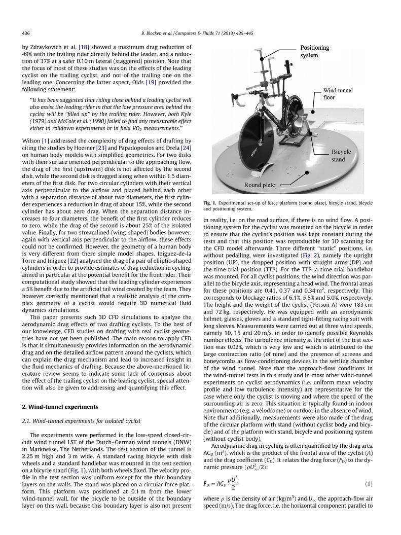
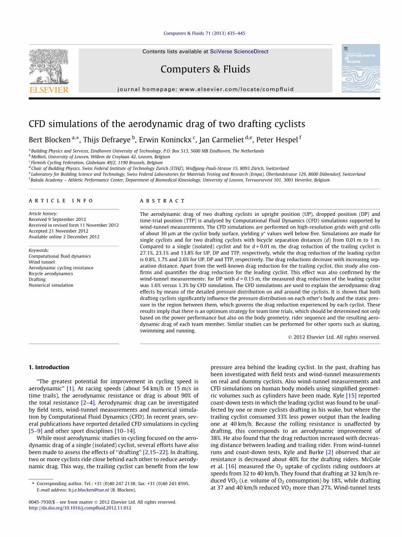
Fig. 1. Experimental set-up of force platform (round plate), bicycle stand, bicycleand positioning system.

436 B. Blocken et al. / Computers & Fluids 71 (2013) 435–445

by Zdravkovich et al. [18] showed a maximum drag reduction of49% with the trailing rider directly behind the leader, and a reduc-tion of 37% at a safer 0.10 m lateral (staggered) position. Note thatthe focus of most of these studies was on the effects of the leadingcyclist on the trailing cyclist, and not of the trailing one on theleading one. Concerning the latter aspect, Olds [19] provided thefollowing statement:

‘‘It has been suggested that riding close behind a leading cyclist willalso assist the leading rider in that the low pressure area behind thecyclist will be ‘‘filled up’’ by the trailing rider. However, both Kyle(1979) and McCole et al. (1990) failed to find any measurable effecteither in rolldown experiments or in field VO2 measurements.’’

Wilson [1] addressed the complexity of drag effects of drafting byciting the studies by Hoerner [23] and Papadopoulos and Drela [24]on human body models with simplified geometries. For two diskswith their surface oriented perpendicular to the approaching flow,the drag of the first (upstream) disk is not affected by the seconddisk, while the second disk is dragged along when within 1.5 diam-eters of the first disk. For two circular cylinders with their verticalaxis perpendicular to the airflow and placed behind each otherwith a separation distance of about two diameters, the first cylin-der experiences a reduction in drag of about 15%, while the secondcylinder has about zero drag. When the separation distance in-creases to four diameters, the benefit of the first cylinder reducesto zero, while the drag of the second is about 25% of the isolatedvalue. Finally, for two streamlined (wing-shaped) bodies however,again with vertical axis perpendicular to the airflow, these effectscould not be confirmed. However, the geometry of a human bodyis very different from these simple model shapes. Iniguez-de-laTorre and Iniguez [22] analysed the drag of a pair of elliptic-shapedcylinders in order to provide estimates of drag reduction in cycling,aimed in particular at the potential benefit for the front rider. Theircomputational study showed that the leading cylinder experiencesa 5% benefit due to the artificial tail wind created by the team. Theyhowever correctly mentioned that a realistic analysis of the com-plex geometry of a cyclist would require 3D numerical fluiddynamics simulations.

This paper presents such 3D CFD simulations to analyse theaerodynamic drag effects of two drafting cyclists. To the best ofour knowledge, CFD studies on drafting with real cyclist geome-tries have not yet been published. The main reason to apply CFDis that it simultaneously provides information on the aerodynamicdrag and on the detailed airflow pattern around the cyclists, whichcan explain the drag mechanism and lead to increased insight inthe fluid mechanics of drafting. Because the above-mentioned lit-erature review seems to indicate some lack of consensus aboutthe effect of the trailing cyclist on the leading cyclist, special atten-tion will also be given to addressing and quantifying this effect.

2. Wind-tunnel experiments

2.1. Wind-tunnel experiments for isolated cyclist

The experiments were performed in the low-speed closed-cir-cuit wind tunnel LST of the Dutch–German wind tunnels (DNW)in Marknesse, The Netherlands. The test section of the tunnel is2.25 m high and 3 m wide. A standard racing bicycle with diskwheels and a standard handlebar was mounted in the test sectionon a bicycle stand (Fig. 1), with both wheels fixed. The velocity pro-file in the test section was uniform except for the thin boundarylayers on the walls. The stand was placed on a circular force plat-form. This platform was positioned at 0.1 m from the lowerwind-tunnel wall, for the bicycle to be outside of the boundarylayer on this wall, because this boundary layer is also not present

in reality, i.e. on the road surface, if there is no wind flow. A posi-tioning system for the cyclist was mounted on the bicycle in orderto ensure that the cyclist’s position was kept constant during thetests and that this position was reproducible for 3D scanning forthe CFD model afterwards. Three different ‘‘static’’ positions, i.e.without pedalling, were investigated (Fig. 2), namely the uprightposition (UP), the dropped position with straight arms (DP) andthe time-trial position (TTP). For the TTP, a time-trial handlebarwas mounted. For all cyclist positions, the wind direction was par-allel to the bicycle axis, representing a head wind. The frontal areasfor these positions are 0.41, 0.37 and 0.34 m2, respectively. Thiscorresponds to blockage ratios of 6.1%, 5.5% and 5.0%, respectively.The height and the weight of the cyclist (Person A) were 183 cmand 72 kg, respectively. He was equipped with an aerodynamichelmet, glasses, gloves and a standard tight-fitting racing suit withlong sleeves. Measurements were carried out at three wind speeds,namely 10, 15 and 20 m/s, in order to identify possible Reynoldsnumber effects. The turbulence intensity at the inlet of the test sec-tion was 0.02%, which is very low and which is attributed to thelarge contraction ratio (of nine) and the presence of screens andhoneycombs as flow-conditioning devices in the settling chamberof the wind tunnel. Note that the approach-flow conditions inthe wind-tunnel tests in this study and in most other wind-tunnelexperiments on cyclist aerodynamics (i.e. uniform mean velocityprofile and low turbulence intensity) are representative for thecase where only the cyclist is moving and where the speed of thesurrounding air is zero. This situation is typically found in indoorenvironments (e.g. a velodrome) or outdoor in the absence of wind.Note that additionally, measurements were also made of the dragof the circular platform with stand (without cyclist body and bicy-cle) and of the platform with stand, bicycle and positioning system(without cyclist body).

Aerodynamic drag in cycling is often quantified by the drag areaACD (m2), which is the product of the frontal area of the cyclist (A)and the drag coefficient (CD). It relates the drag force (FD) to the dy-namic pressure ðqU2

1=2Þ:

FD ¼ ACDqU2

12

ð1Þ

where q is the density of air (kg/m3) and U1 the approach-flow airspeed (m/s). The drag force, i.e. the horizontal component parallel to

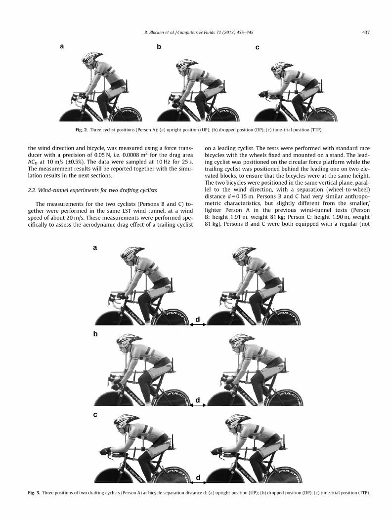
Fig. 2. Three cyclist positions (Person A): (a) upright position (UP); (b) dropped position (DP); (c) time-trial position (TTP).

B. Blocken et al. / Computers & Fluids 71 (2013) 435–445 437

the wind direction and bicycle, was measured using a force trans-ducer with a precision of 0.05 N, i.e. 0.0008 m2 for the drag areaACD at 10 m/s (±0.5%). The data were sampled at 10 Hz for 25 s.The measurement results will be reported together with the simu-lation results in the next sections.

2.2. Wind-tunnel experiments for two drafting cyclists

The measurements for the two cyclists (Persons B and C) to-gether were performed in the same LST wind tunnel, at a windspeed of about 20 m/s. These measurements were performed spe-cifically to assess the aerodynamic drag effect of a trailing cyclist

Fig. 3. Three positions of two drafting cyclists (Person A) at bicycle separation distance

on a leading cyclist. The tests were performed with standard racebicycles with the wheels fixed and mounted on a stand. The lead-ing cyclist was positioned on the circular force platform while thetrailing cyclist was positioned behind the leading one on two ele-vated blocks, to ensure that the bicycles were at the same height.The two bicycles were positioned in the same vertical plane, paral-lel to the wind direction, with a separation (wheel-to-wheel)distance d = 0.15 m. Persons B and C had very similar anthropo-metric characteristics, but slightly different from the smaller/lighter Person A in the previous wind-tunnel tests (PersonB: height 1.91 m, weight 81 kg; Person C: height 1.90 m, weight81 kg). Persons B and C were both equipped with a regular (not

d: (a) upright position (UP); (b) dropped position (DP); (c) time-trial position (TTP).


time-trial) helmet and a standard racing suit with long sleeves.Measurements were only made for both cyclists in DP. Addition-ally, measurements were also made of the drag of the circular plat-form with stand (without cyclist body and bicycle) and of theplatform with stand and bicycle (without cyclist body). The mea-surement results will be reported together with the simulation re-sults in the next sections.

3. Numerical simulations: computational settings andparameters

3.1. Computational geometry and domain

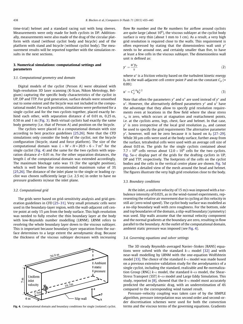
Digital models of the cyclist (Person A) were obtained withhigh-resolution 3D laser scanning (K-Scan, Nikon Metrology, Bel-gium) capturing the specific body characteristics of the cyclist inUP, DP and TTP. For grid generation, surface details were smoothedout to some extent and the bicycle was not included in the compu-tational model. For each position, simulations were performed for asingle cyclist and for the two cyclists together, placed exactly be-hind each other, with separation distance d of 0.01 m, 0.25 m,0.50 m and 1 m (Fig. 3). Both virtual cyclists had exactly the samebody geometry (i.e. that of Person A) and position on the bicycle.

The cyclists were placed in a computational domain with sizeaccording to best practice guidelines [25,26]. Note that the CFDsimulations only consider the body of the cyclist, not the bicycleconfiguration (bicycle, stand and force platform). The size of thecomputational domain was L �W � H = 20.9 � 6 � 7 m3 for thesingle cyclist (Fig. 4) and the same for the two cyclists with sepa-ration distance d = 0.01 m. For the other separation distances, thelength L of the computational domain was extended accordingly.The maximum blockage ratio was 1% (for the upright position),which is well below the recommended maximum value of 3%[25,26]. The distance of the inlet plane to the single or leading cy-clist was chosen sufficiently large (i.e. 2.5 m) in order to have nopressure gradients in/near the inlet plane.

3.2. Computational grid

The grids were based on grid-sensitivity analysis and grid-gen-eration guidelines in CFD [25–31]. Very small prismatic cells wereused in the boundary-layer region, with the wall-adjacent cell cen-tre point at only 15 lm from the body surface. This high resolutionwas needed to fully resolve the thin boundary layer at the bodywith low-Reynolds number modelling (LRNM). LRNM refers toresolving the whole boundary layer down to the viscous sublayer.This is important because boundary layer separation from the sur-face determines to a large extent the aerodynamic drag. Becausethe thickness of the viscous sublayer decreases with increasing

Fig. 4. Computational domain and boundary conditions for single (isolated) cyclist.

flow Re number and the Re numbers for airflow around cyclistsare quite large (about 106), the viscous sublayer at the cyclist bodysurface is very thin (about 1 mm to 1 cm). As a result, a very highgrid resolution is required close to the walls. This requirement isoften expressed by stating that the dimensionless wall unit y⁄

needs to be around one, and certainly smaller than five, to haveat least a few cells in the viscous sublayer. The dimensionless wallunit is defined as:

y� ¼ u�yP

mð2Þ

where u⁄ is a friction velocity based on the turbulent kinetic energykP in the wall-adjacent cell centre point P and on the constant Cl (=0.09):

u� ¼ C1=4l k1=2

P ð3Þ

Note that often the parameters y+ and u+ are used instead of y⁄ andu⁄. However, the alternatively defined parameters y⁄ and u⁄ havethe advantage that they allow to specify grid resolution require-ments even at locations in the flow field where the shear stresssw is zero, which occurs at stagnation and reattachment points,i.e. at the cyclists arms, legs, chest, face and helmet. In that case,y+ is zero irrespective of the local grid resolution yP, and cannotbe used to specify the grid requirements The alternative parametery⁄, however, will not be zero because it is based on kP [27–29].While 30 lm cells were used at the body surface, further away fromthe surface, tetrahedral cells were used with an average cell size ofabout 0.03 m. The grids for the single cyclists contained about7.7 � 106 cells versus about 12.0 � 106 cells for the two cyclists.Fig. 5a–c display part of the grids for the drafting cyclists in UP,DP and TTP, respectively. The footprints of the cells on the cyclistbodies and the cells in the vertical centre plane are shown. Fig. 5dprovides a detailed view of the mesh around the head and helmet.The figures illustrate the very high grid resolution close to the body.

3.3. Boundary conditions

At the inlet, a uniform velocity of 15 m/s was imposed with a tur-bulence intensity of 0.02%, as in the wind-tunnel experiments, rep-resenting the relative air movement due to cycling at this velocity instill air (zero wind speed). The cyclist body surface was modelled asa no-slip boundary wall with zero roughness. For the bottom, sideand top boundaries of the domain, a slip-wall boundary (symmetry)was used. Slip walls assume that the normal velocity componentand the normal gradients at the boundary are zero, resulting in flowparallel to the boundary. At the outlet of the computational domain,ambient static pressure was imposed (see Fig. 4).

3.4. Governing equations and solver settings

The 3D steady Reynolds-averaged Navier–Stokes (RANS) equa-tions were solved with the standard k–e model [32] and withnear-wall modelling by LRNM with the one-equation Wolfshteinmodel [33]. The choice of the standard k–e model was made basedon a previous extensive validation study for the aerodynamics of asingle cyclist, including the standard, realizable and Re-normaliza-tion Group (RNG) k–e model, the standard k–x model, the Shear-Stress Transport (SST) k–x model and Large Eddy Simulation. Thisstudy, reported in [8], showed that the k–e model most accuratelypredicted the aerodynamic drag, with an underestimation of 4%compared to the corresponding wind tunnel result.

Pressure–velocity coupling was taken care of by the SIMPLEalgorithm, pressure interpolation was second order and second-or-der discretisation schemes were used for both the convectionterms and the viscous terms of the governing equations. Gradients

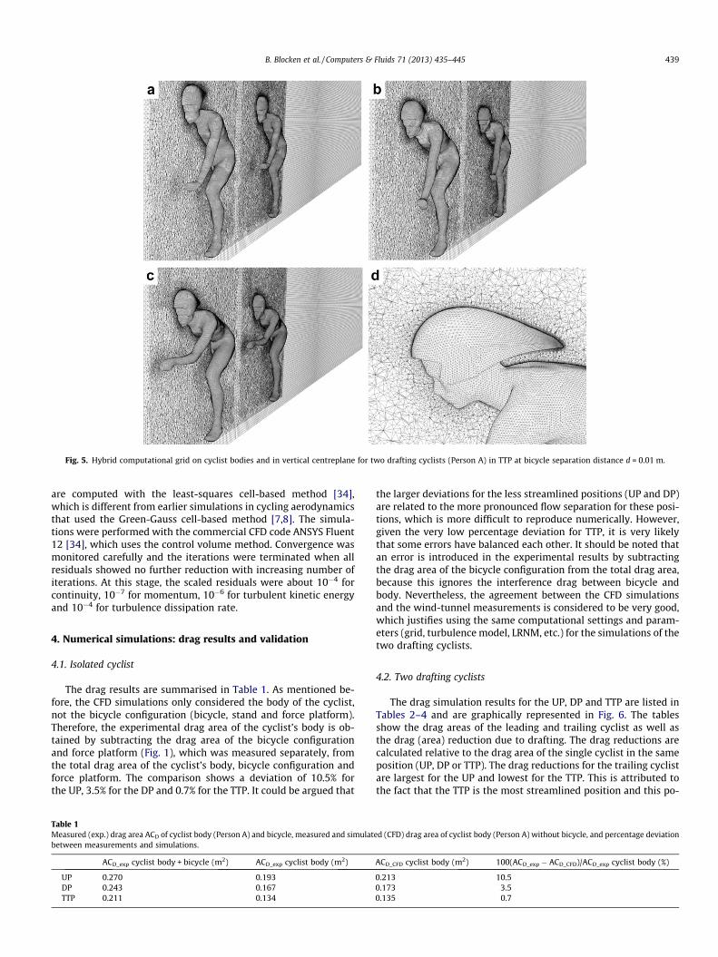
Fig. 5. Hybrid computational grid on cyclist bodies and in vertical centreplane for two drafting cyclists (Person A) in TTP at bicycle separation distance d = 0.01 m.


are computed with the least-squares cell-based method [34],which is different from earlier simulations in cycling aerodynamicsthat used the Green-Gauss cell-based method [7,8]. The simula-tions were performed with the commercial CFD code ANSYS Fluent12 [34], which uses the control volume method. Convergence wasmonitored carefully and the iterations were terminated when allresiduals showed no further reduction with increasing number ofiterations. At this stage, the scaled residuals were about 10�4 forcontinuity, 10�7 for momentum, 10�6 for turbulent kinetic energyand 10�4 for turbulence dissipation rate.

4. Numerical simulations: drag results and validation

4.1. Isolated cyclist

The drag results are summarised in Table 1. As mentioned be-fore, the CFD simulations only considered the body of the cyclist,not the bicycle configuration (bicycle, stand and force platform).Therefore, the experimental drag area of the cyclist’s body is ob-tained by subtracting the drag area of the bicycle configurationand force platform (Fig. 1), which was measured separately, fromthe total drag area of the cyclist’s body, bicycle configuration andforce platform. The comparison shows a deviation of 10.5% forthe UP, 3.5% for the DP and 0.7% for the TTP. It could be argued that

Table 1Measured (exp.) drag area ACD of cyclist body (Person A) and bicycle, measured and simulatbetween measurements and simulations.

ACD_exp cyclist body + bicycle (m2) ACD_exp cyclist body (m2)

UP 0.270 0.193DP 0.243 0.167TTP 0.211 0.134

the larger deviations for the less streamlined positions (UP and DP)are related to the more pronounced flow separation for these posi-tions, which is more difficult to reproduce numerically. However,given the very low percentage deviation for TTP, it is very likelythat some errors have balanced each other. It should be noted thatan error is introduced in the experimental results by subtractingthe drag area of the bicycle configuration from the total drag area,because this ignores the interference drag between bicycle andbody. Nevertheless, the agreement between the CFD simulationsand the wind-tunnel measurements is considered to be very good,which justifies using the same computational settings and param-eters (grid, turbulence model, LRNM, etc.) for the simulations of thetwo drafting cyclists.

4.2. Two drafting cyclists

The drag simulation results for the UP, DP and TTP are listed inTables 2–4 and are graphically represented in Fig. 6. The tablesshow the drag areas of the leading and trailing cyclist as well asthe drag (area) reduction due to drafting. The drag reductions arecalculated relative to the drag area of the single cyclist in the sameposition (UP, DP or TTP). The drag reductions for the trailing cyclistare largest for the UP and lowest for the TTP. This is attributed tothe fact that the TTP is the most streamlined position and this po-

ed (CFD) drag area of cyclist body (Person A) without bicycle, and percentage deviation

ACD_CFD cyclist body (m2) 100(ACD_exp � ACD_CFD)/ACD_exp cyclist body (%)

0.213 10.50.173 3.50.135 0.7

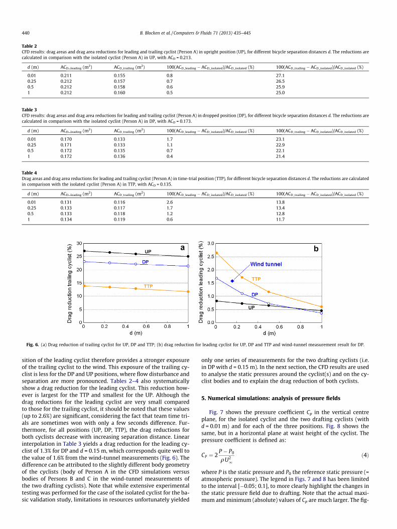
Table 2CFD results: drag areas and drag area reductions for leading and trailing cyclist (Person A) in upright position (UP), for different bicycle separation distances d. The reductions arecalculated in comparison with the isolated cyclist (Person A) in UP, with ACD = 0.213.

d (m) ACD_leading (m2) ACD_trailing (m2) 100(ACD_leading � ACD_isolated)/ACD_isolated (%) 100(ACD_trailing � ACD_isolated)/ACD_isolated (%)

0.01 0.211 0.155 0.8 27.10.25 0.212 0.157 0.7 26.50.5 0.212 0.158 0.6 25.91 0.212 0.160 0.5 25.0

Table 3CFD results: drag areas and drag area reductions for leading and trailing cyclist (Person A) in dropped position (DP), for different bicycle separation distances d. The reductions arecalculated in comparison with the isolated cyclist (Person A) in DP, with ACD = 0.173.


0.01 0.170 0.133 1.7 23.10.25 0.171 0.133 1.1 22.90.5 0.172 0.135 0.7 22.11 0.172 0.136 0.4 21.4

Table 4Drag areas and drag area reductions for leading and trailing cyclist (Person A) in time-trial position (TTP), for different bicycle separation distances d. The reductions are calculatedin comparison with the isolated cyclist (Person A) in TTP, with ACD = 0.135.


0.01 0.131 0.116 2.6 13.80.25 0.133 0.117 1.7 13.40.5 0.133 0.118 1.2 12.81 0.134 0.119 0.6 11.7

Fig. 6. (a) Drag reduction of trailing cyclist for UP, DP and TTP; (b) drag reduction for leading cyclist for UP, DP and TTP and wind-tunnel measurement result for DP.


sition of the leading cyclist therefore provides a stronger exposureof the trailing cyclist to the wind. This exposure of the trailing cy-clist is less for the DP and UP positions, where flow disturbance andseparation are more pronounced. Tables 2–4 also systematicallyshow a drag reduction for the leading cyclist. This reduction how-ever is largest for the TTP and smallest for the UP. Although thedrag reductions for the leading cyclist are very small comparedto those for the trailing cyclist, it should be noted that these values(up to 2.6%) are significant, considering the fact that team time tri-als are sometimes won with only a few seconds difference. Fur-thermore, for all positions (UP, DP, TTP), the drag reductions forboth cyclists decrease with increasing separation distance. Linearinterpolation in Table 3 yields a drag reduction for the leading cy-clist of 1.3% for DP and d = 0.15 m, which corresponds quite well tothe value of 1.6% from the wind-tunnel measurements (Fig. 6). Thedifference can be attributed to the slightly different body geometryof the cyclists (body of Person A in the CFD simulations versusbodies of Persons B and C in the wind-tunnel measurements ofthe two drafting cyclists). Note that while extensive experimentaltesting was performed for the case of the isolated cyclist for the ba-sic validation study, limitations in resources unfortunately yielded

only one series of measurements for the two drafting cyclists (i.e.in DP with d = 0.15 m). In the next section, the CFD results are usedto analyse the static pressures around the cyclist(s) and on the cy-clist bodies and to explain the drag reduction of both cyclists.

5. Numerical simulations: analysis of pressure fields

Fig. 7 shows the pressure coefficient Cp in the vertical centreplane, for the isolated cyclist and the two drafting cyclists (withd = 0.01 m) and for each of the three positions. Fig. 8 shows thesame, but in a horizontal plane at waist height of the cyclist. Thepressure coefficient is defined as:

CP ¼ 2P � P0

qU21

ð4Þ

where P is the static pressure and P0 the reference static pressure (=atmospheric pressure). The legend in Figs. 7 and 8 has been limitedto the interval [�0.05; 0.1], to more clearly highlight the changes inthe static pressure field due to drafting. Note that the actual maxi-mum and minimum (absolute) values of Cp are much larger. The fig-

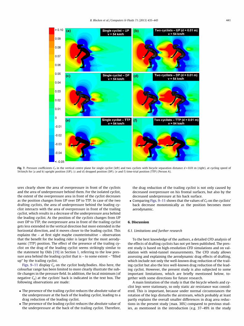
Fig. 7. Pressure coefficients CP in the vertical centre plane for single cyclist (left) and two cyclists with bicycle separation distance d = 0.01 m (right), at cycling speed of54 km/h for (a and b) upright position (UP); (c and d) dropped position (DP); (e and f) time-trial position (TTP) (Person A).


ures clearly show the area of overpressure in front of the cyclistsand the area of underpressure behind them. For the isolated cyclist,the extent of the overpressure area in front of the cyclist decreasesas the position changes from UP over DP to TTP. In case of the twodrafting cyclists, the area of underpressure behind the leading cy-clist interacts with the area of overpressure in front of the trailingcyclist, which results in a decrease of the underpressure area behindthe leading cyclist. As the position of the cyclists changes from UPover DP to TTP, the overpressure area in front of the trailing cyclistgets less extended in the vertical direction but more extended in thehorizontal direction, and it moves closer to the leading cyclist. Thisexplains the – at first sight maybe counterintuitive – observationthat the benefit for the leading rider is larger for the most aerody-namic (TTP) position. The effect of the presence of the trailing cy-clist on the drag of the leading cyclist seems strikingly similar tothe statement by Olds [19] in Section 1, referring to the low pres-sure area behind the leading cyclist that is – to some extent – ‘‘filledup’’ by the trailing cyclist.

Figs. 9–11 display Cp on the cyclist body/bodies. Also here, thecolourbar range has been limited to more clearly illustrate the sub-tle changes in the pressure field. In addition, the local minimum (ofnegative Cp) at the cyclists’ back is indicated in the text box. Thefollowing observations are made:

� The presence of the trailing cyclist reduces the absolute value ofthe underpressure at the back of the leading cyclist, leading to adrag reduction of the leading cyclist.� The presence of the leading cyclist reduces the absolute value of

the underpressure at the back of the trailing cyclist. Therefore,

the drag reduction of the trailing cyclist is not only caused bydecreased overpressure on his frontal surfaces, but also by thedecreased underpressure at his back surface.� Comparing Figs. 9–11 shows that the values of CP on the cyclists’

back decrease monotonically as the position becomes moreaerodynamic.

6. Discussion

6.1. Limitations and further research

To the best knowledge of the authors, a detailed CFD analysis ofthe effects of drafting cyclists has not yet been published. The pres-ent study is based on high-resolution CFD simulations and on val-idation with wind-tunnel measurements. The CFD study allowsassessing and explaining the aerodynamic drag effects of drafting,which include not only the well-known drag reduction of the trail-ing cyclist but also the less well-known drag reduction of the lead-ing cyclist. However, the present study is also subjected to someimportant limitations, which are briefly mentioned below, to-gether with some directions for future research.

A main limitation of the study is that the bicycle wheels and cy-clist legs were stationary, so only static air resistance was consid-ered. This is important, because under normal circumstances therotation of the legs disturbs the airstream, which probably at leastpartly explains the overall smaller differences in drag area reduc-tions in the present study (max. 30%) compared to previous stud-ies, as mentioned in the introduction (e.g. 37–49% in the study

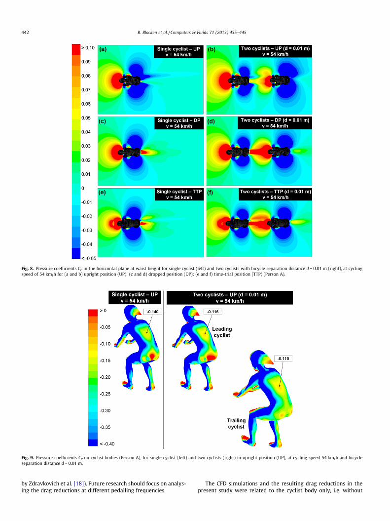
Fig. 8. Pressure coefficients CP in the horizontal plane at waist height for single cyclist (left) and two cyclists with bicycle separation distance d = 0.01 m (right), at cyclingspeed of 54 km/h for (a and b) upright position (UP); (c and d) dropped position (DP); (e and f) time-trial position (TTP) (Person A).

Fig. 9. Pressure coefficients CP on cyclist bodies (Person A), for single cyclist (left) and two cyclists (right) in upright position (UP), at cycling speed 54 km/h and bicycleseparation distance d = 0.01 m.


by Zdravkovich et al. [18]). Future research should focus on analys-ing the drag reductions at different pedalling frequencies.

The CFD simulations and the resulting drag reductions in thepresent study were related to the cyclist body only, i.e. without

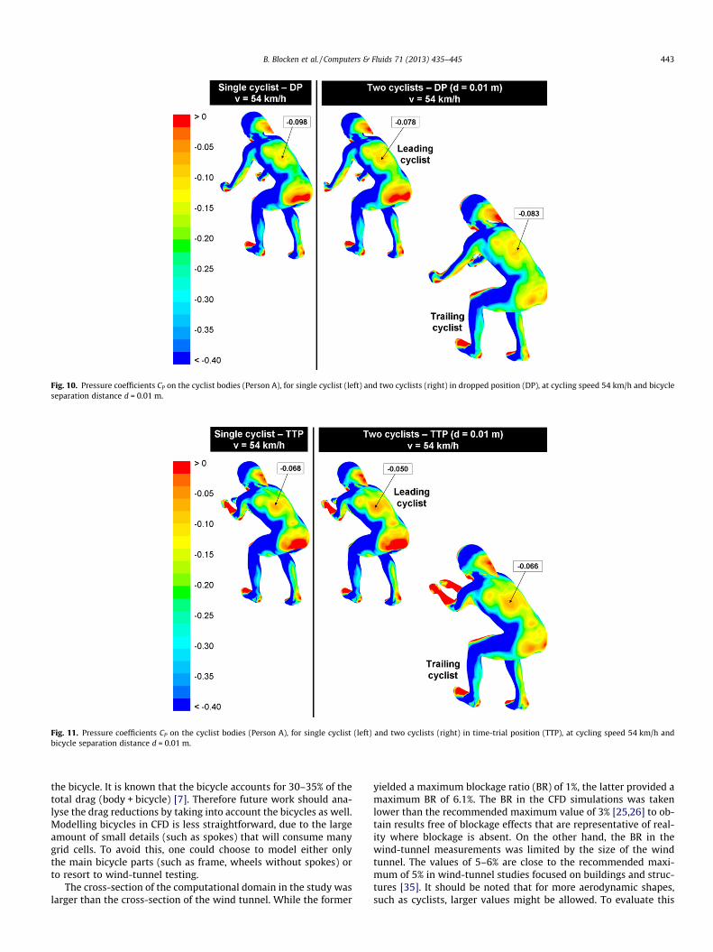
Fig. 10. Pressure coefficients CP on the cyclist bodies (Person A), for single cyclist (left) and two cyclists (right) in dropped position (DP), at cycling speed 54 km/h and bicycleseparation distance d = 0.01 m.

Fig. 11. Pressure coefficients CP on the cyclist bodies (Person A), for single cyclist (left) and two cyclists (right) in time-trial position (TTP), at cycling speed 54 km/h andbicycle separation distance d = 0.01 m.


the bicycle. It is known that the bicycle accounts for 30–35% of thetotal drag (body + bicycle) [7]. Therefore future work should ana-lyse the drag reductions by taking into account the bicycles as well.Modelling bicycles in CFD is less straightforward, due to the largeamount of small details (such as spokes) that will consume manygrid cells. To avoid this, one could choose to model either onlythe main bicycle parts (such as frame, wheels without spokes) orto resort to wind-tunnel testing.

The cross-section of the computational domain in the study waslarger than the cross-section of the wind tunnel. While the former

yielded a maximum blockage ratio (BR) of 1%, the latter provided amaximum BR of 6.1%. The BR in the CFD simulations was takenlower than the recommended maximum value of 3% [25,26] to ob-tain results free of blockage effects that are representative of real-ity where blockage is absent. On the other hand, the BR in thewind-tunnel measurements was limited by the size of the windtunnel. The values of 5–6% are close to the recommended maxi-mum of 5% in wind-tunnel studies focused on buildings and struc-tures [35]. It should be noted that for more aerodynamic shapes,such as cyclists, larger values might be allowed. To evaluate this

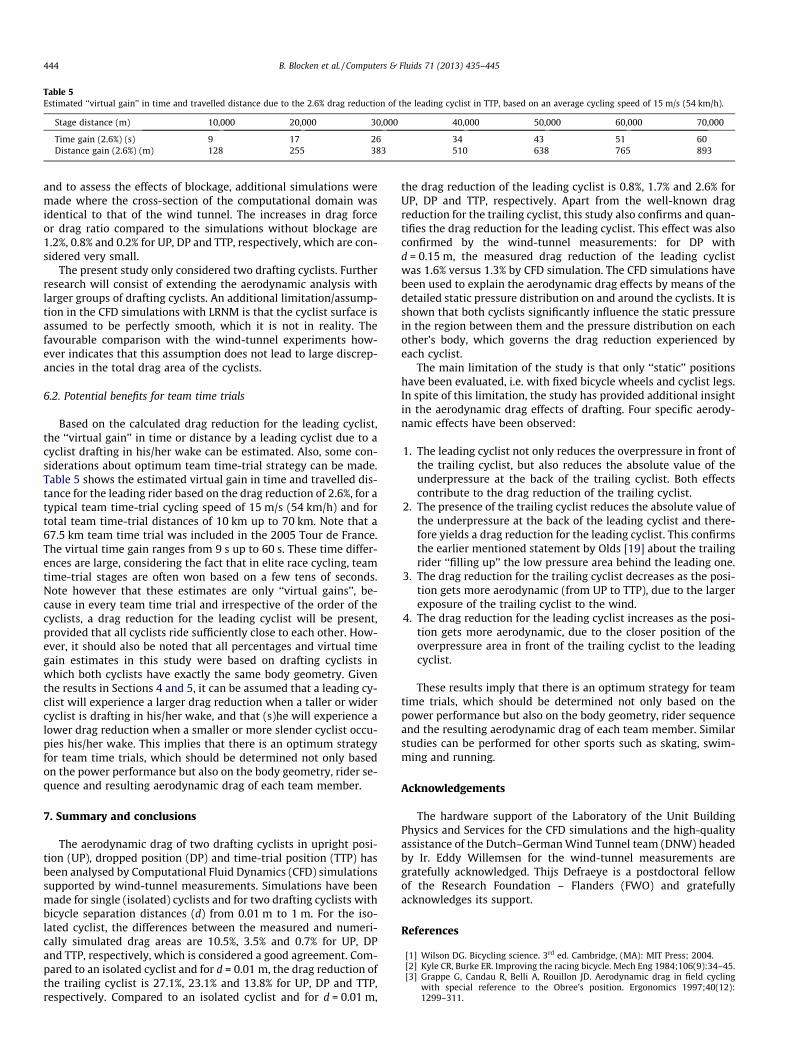
Table 5Estimated ‘‘virtual gain’’ in time and travelled distance due to the 2.6% drag reduction of the leading cyclist in TTP, based on an average cycling speed of 15 m/s (54 km/h).

Stage distance (m) 10,000 20,000 30,000 40,000 50,000 60,000 70,000

Time gain (2.6%) (s) 9 17 26 34 43 51 60Distance gain (2.6%) (m) 128 255 383 510 638 765 893


and to assess the effects of blockage, additional simulations weremade where the cross-section of the computational domain wasidentical to that of the wind tunnel. The increases in drag forceor drag ratio compared to the simulations without blockage are1.2%, 0.8% and 0.2% for UP, DP and TTP, respectively, which are con-sidered very small.

The present study only considered two drafting cyclists. Furtherresearch will consist of extending the aerodynamic analysis withlarger groups of drafting cyclists. An additional limitation/assump-tion in the CFD simulations with LRNM is that the cyclist surface isassumed to be perfectly smooth, which it is not in reality. Thefavourable comparison with the wind-tunnel experiments how-ever indicates that this assumption does not lead to large discrep-ancies in the total drag area of the cyclists.

6.2. Potential benefits for team time trials

Based on the calculated drag reduction for the leading cyclist,the ‘‘virtual gain’’ in time or distance by a leading cyclist due to acyclist drafting in his/her wake can be estimated. Also, some con-siderations about optimum team time-trial strategy can be made.Table 5 shows the estimated virtual gain in time and travelled dis-tance for the leading rider based on the drag reduction of 2.6%, for atypical team time-trial cycling speed of 15 m/s (54 km/h) and fortotal team time-trial distances of 10 km up to 70 km. Note that a67.5 km team time trial was included in the 2005 Tour de France.The virtual time gain ranges from 9 s up to 60 s. These time differ-ences are large, considering the fact that in elite race cycling, teamtime-trial stages are often won based on a few tens of seconds.Note however that these estimates are only ‘‘virtual gains’’, be-cause in every team time trial and irrespective of the order of thecyclists, a drag reduction for the leading cyclist will be present,provided that all cyclists ride sufficiently close to each other. How-ever, it should also be noted that all percentages and virtual timegain estimates in this study were based on drafting cyclists inwhich both cyclists have exactly the same body geometry. Giventhe results in Sections 4 and 5, it can be assumed that a leading cy-clist will experience a larger drag reduction when a taller or widercyclist is drafting in his/her wake, and that (s)he will experience alower drag reduction when a smaller or more slender cyclist occu-pies his/her wake. This implies that there is an optimum strategyfor team time trials, which should be determined not only basedon the power performance but also on the body geometry, rider se-quence and resulting aerodynamic drag of each team member.

7. Summary and conclusions

The aerodynamic drag of two drafting cyclists in upright posi-tion (UP), dropped position (DP) and time-trial position (TTP) hasbeen analysed by Computational Fluid Dynamics (CFD) simulationssupported by wind-tunnel measurements. Simulations have beenmade for single (isolated) cyclists and for two drafting cyclists withbicycle separation distances (d) from 0.01 m to 1 m. For the iso-lated cyclist, the differences between the measured and numeri-cally simulated drag areas are 10.5%, 3.5% and 0.7% for UP, DPand TTP, respectively, which is considered a good agreement. Com-pared to an isolated cyclist and for d = 0.01 m, the drag reduction ofthe trailing cyclist is 27.1%, 23.1% and 13.8% for UP, DP and TTP,respectively. Compared to an isolated cyclist and for d = 0.01 m,

the drag reduction of the leading cyclist is 0.8%, 1.7% and 2.6% forUP, DP and TTP, respectively. Apart from the well-known dragreduction for the trailing cyclist, this study also confirms and quan-tifies the drag reduction for the leading cyclist. This effect was alsoconfirmed by the wind-tunnel measurements: for DP withd = 0.15 m, the measured drag reduction of the leading cyclistwas 1.6% versus 1.3% by CFD simulation. The CFD simulations havebeen used to explain the aerodynamic drag effects by means of thedetailed static pressure distribution on and around the cyclists. It isshown that both cyclists significantly influence the static pressurein the region between them and the pressure distribution on eachother’s body, which governs the drag reduction experienced byeach cyclist.

The main limitation of the study is that only ‘‘static’’ positionshave been evaluated, i.e. with fixed bicycle wheels and cyclist legs.In spite of this limitation, the study has provided additional insightin the aerodynamic drag effects of drafting. Four specific aerody-namic effects have been observed:

1. The leading cyclist not only reduces the overpressure in front ofthe trailing cyclist, but also reduces the absolute value of theunderpressure at the back of the trailing cyclist. Both effectscontribute to the drag reduction of the trailing cyclist.

2. The presence of the trailing cyclist reduces the absolute value ofthe underpressure at the back of the leading cyclist and there-fore yields a drag reduction for the leading cyclist. This confirmsthe earlier mentioned statement by Olds [19] about the trailingrider ‘‘filling up’’ the low pressure area behind the leading one.

3. The drag reduction for the trailing cyclist decreases as the posi-tion gets more aerodynamic (from UP to TTP), due to the largerexposure of the trailing cyclist to the wind.

4. The drag reduction for the leading cyclist increases as the posi-tion gets more aerodynamic, due to the closer position of theoverpressure area in front of the trailing cyclist to the leadingcyclist.

These results imply that there is an optimum strategy for teamtime trials, which should be determined not only based on thepower performance but also on the body geometry, rider sequenceand the resulting aerodynamic drag of each team member. Similarstudies can be performed for other sports such as skating, swim-ming and running.

Acknowledgements

The hardware support of the Laboratory of the Unit BuildingPhysics and Services for the CFD simulations and the high-qualityassistance of the Dutch–German Wind Tunnel team (DNW) headedby Ir. Eddy Willemsen for the wind-tunnel measurements aregratefully acknowledged. Thijs Defraeye is a postdoctoral fellowof the Research Foundation – Flanders (FWO) and gratefullyacknowledges its support.

References

[1] Wilson DG. Bicycling science. 3rd ed. Cambridge, (MA): MIT Press; 2004.[2] Kyle CR, Burke ER. Improving the racing bicycle. Mech Eng 1984;106(9):34–45.[3] Grappe G, Candau R, Belli A, Rouillon JD. Aerodynamic drag in field cycling

with special reference to the Obree’s position. Ergonomics 1997;40(12):1299–311.


[4] Lukes RA, Chin SB, Haake SJ. The understanding and development of cyclingaerodynamics. Sports Eng 2005;8:59–74.

[5] Hanna RK. Can CFD make a performance difference in sport? In: Ujihashi S,Haake SJ, editors. The Engineering of Sport 4. Oxford: Blackwell Science; 2002.p. 17–30.

[6] Lukes RA, Hart JH, Chin SB, Haake SJ. The aerodynamics of mountain bicycles:the role of computational fluid dynamics. In: Hubbard M, Mehta RD, Pallis JM,editors. The engineering of sport 5. Sheffield: International Sports EngAssociation; 2004.

[7] Defraeye T, Blocken B, Koninckx E, Hespel P, Carmeliet J. Aerodynamic study ofdifferent cyclist positions: CFD analysis and full-scale wind-tunnel tests. JBiomech 2010;43(7):1262–8.

[8] Defraeye T, Blocken B, Koninckx E, Hespel P, Carmeliet J. Computational fluiddynamics analysis of cyclist aerodynamics: performance of differentturbulence-modelling and boundary-layer modelling approaches. J Biomech2010;43(12):2281–7.

[9] Defraeye T, Blocken B, Koninckx E, Hespel P, Carmeliet J. Computational fluiddynamics analysis of drag and convective heat transfer of individual bodysegments for different cyclist positions. J Biomech 2011;44(9):1695–701.

[10] Dabnichki P, Avital E. Influence of the position of crew members onaerodynamics performance of a two-man bobsleigh. J Biomech 2006;39(15):2733–42.

[11] Lecrivain G, Slaouti A, Payton C, Kennedy I. Using reverse engineering andcomputational fluid dynamics to investigate a lower arm amputee swimmer’sperformance. J Biomech 2008;41(13):2855–9.

[12] Zaïdi H, Taiar R, Fohanno S, Polidori G. Analysis of the effect of swimmer’s headposition on swimming performance using computational fluid dynamics. JBiomech 2008;41(6):1350–8.

[13] Minetti AE, Machtsiras G, Masters JC. The optimum finger spacing in humanswimming. J Biomech 2009;42:2188–90.

[14] Zaïdi H, Fohanno S, Taiar R, Polidori G. Turbulence model choice for thecalculation of drag forces when using the CFD method. J Biomech2010;43(3):405–11.

[15] Kyle CR. Reduction of wind resistance and power output of racing cyclists andrunnings travelling in groups. Ergonomics 1979;22(4):387–97.

[16] McCole SD, Claney K, Conte J-C, Anderson R, Hagberg JM. Energy expenditureduring bicycling. J Appl Physiol 1990;68(2):748–53.

[17] Hagberg JM, McCole SD. The effect of drafting and aerodynamic equipment onthe energy expenditure during cycling. Cycl Sci 1990;2(3):19–22.

[18] Zdravkovich MM, Ashcroft MW, Chisholm SJ, Hicks N. Effect of cyclist’s postureand vicinity of another cyclist on aerodynamic drag. In: Haake, editor. Theengineering of sport. Rotterdam: Balkema; 1996. p. 21–8.

[19] Olds T. The mathematics of breaking away and chasing in cycling. Eur J ApplPhysiol 1998;77:492–7.

[20] Broker JP, Kyle CR, Burke ER. Racing cyclist power requirements in the 4000-mindividual and team pursuits. Med Sci Sports Exercise 1999;31(11):1677–85.

[21] Edwards AG, Byrnes WC. Aerodynamic characteristics as determinants of thedrafting effect in cycling. Med Sci Sports Exercise 2007;39(1):170–6.

[22] Iniguez-de-la-Torre A, Iniguez J. Aerodynamics of a cycling team in a time trial:does the cyclist at the front benefit? Eur J Phys 2009;30:1365–9.

[23] Hoerner SF. 1965. Fluid dynamic drag. Bricktown, NJ.[24] Papadopoulos J, Drela M. Some comment on the effects of interference drag on

two bodies in tandem and side-by-side. Human Power 1999;46:19–20.[25] Franke J, Hellsten A, Schlünzen H, Carissimo B. Best practice guideline for the

CFD simulation of flows in the urban environment, COST Action 732: qualityassurance and improvement of microscale meteorological models. Germany:Hamburg; 2007.

[26] Tominaga Y, Mochida A, Yoshie R, Kataoka H, Nozu T, Yoshikawa M, et al. AIJguidelines for practical applications of CFD to pedestrian wind environmentaround buildings. J Wind Eng Ind Aerodyn 2008;96(10–11):1749–61.

[27] Casey M, Wintergerste T. Best practice guidelines. ERCOFTAC Special interestgroup on ‘‘quality and trust in industrial CFD’’, ERCOFTAC 2000.

[28] Blocken B, Defraeye T, Derome D, Carmeliet J. High-resolution CFD simulationsof forced convective heat transfer coefficients at the facade of a low-risebuilding. Build Environ 2009;44(12):2396–412.

[29] Defraeye T, Blocken B, Carmeliet J. CFD analysis of convective heat transfer atthe surfaces of a cube immersed in a turbulent boundary layer. Int J Heat MassTrans 2010;53(1–3):297–308.

[30] Blocken B, Janssen WD, van Hooff T. CFD simulation for pedestrian windcomfort and wind safety in urban areas: general decision framework and casestudy for the Eindhoven University campus. Environ Modell Softw2012;30:15–34.

[31] Blocken B, Gualtieri C. Ten iterative steps for model development andevaluation applied to computational fluid dynamics for environmental fluidmechanics. Environ Modell Softw 2012;33:1–22.

[32] Jones WP, Launder BE. The prediction of laminarization with a two-equationmodel of turbulence. Int J Heat Mass Transfer 1972;15:301–14.

[33] Wolfshtein M. The velocity and temperature distribution in one-dimensionalflow with turbulence augmentation and pressure gradient. Int J Heat MassTransfer 1969;12(3):301–18.

[34] ANSYS Inc. 2009. ANSYS Fluent 12.0 theory guide.[35] ASCE 1999. Wind tunnel studies of buildings and structures. N. Isyumov (Ed.),

ASCE manuals and reports on engineering practice No. 67, American Society ofCivil Engineers, 214 pp.

cfd simulations of the aerodynamic drag of two drafting … · · 2017-12-25cfd simulations of...

Documents