UCRL-JC-138310 PREPRINT

Aerodynamic Drag of Heavy Vehicles (Class 7-8): Simulation and Benchmarking

Rose McCallen, Dan Flowers, Tim Dunn, Jerry Owens Fred Browand, Mustapha Hammache, University Southern California

Anthony Leonard, Mark Brady, California Institute of Technology Kambiz Salari, Walter Rutledge, Sandia National Laboratories

James Ross, Bruce Storms”, J.T. Heineck, David Driver, James Bell, Steve Walker, Gregory Zilliac, NASA Ames Research Center

“On contract to NASA from Aerospace Computing, Inc.

This paper was prepared for submittal to Society of Automotive Engineers Government Industry Meeting

June 19-Z&2000 Washington, DC

March 31,ZOOO

DISCLAIMER

This document was prepared as an account of work sponsored by an agency of the United States Government. Neither the United States Government nor the University of California nor any of their employees, makes any warranty, express or implied, or assumes any legal liability or responsibility for the accuracy, completeness, or usefulness of any information, apparatus, product, or process disclosed, or represents that its use would not infringe privately owned rights. Reference herein to any specific commercial product, process, or service by trade name, trademark, manufacturer, or otherwise, does not necessarily constitute or imply its endorsement, recommendation, or favoring by the United States Government or the University of California. The views and opinions of authors expressed herein do not necessarily state or reflect those of the United States Government or the University of California, and shall not be used for advertising or product endorsement purposes.

Aerodyna mic Drag of Heavy Vehicles (Class 7-8): Simulation and Benchmarking

Paper Number

Rose McCallen, Dan Flowers, Tim Dunn, Jerry Owens Lawrence Livermore National Laboratory

Fred Browand and Mustapha Hammache University of Southern California

Anthony Leonard and Mark Brady California Institute of Technology

Kambiz Salari and Walter Rutledge Sandia National Laboratories

James Ross, Bruce Storms*, J.T. Heineck, David Driver, James Bell, Steve Walker, Gregory Zilliac

NASA Ames Research Center * On contract to NASAAmes from Aerospace Computing, Inc.

Copyright 0 1998 Society ofAutomotive Engineers, Inc

ABSTRACT

This paper describes research and development for reducing the aerodynamic drag of heavy vehicles by demonstrating new approaches for the numerical simula- tion and analysis of aerodynamic flow. Experimental vali- dation of new computational fluid dynamics methods are also an important part of this approach. Experiments on a model of an integrated tractor-trailer are underway at NASA Ames Research Center and the University of Southern California (USC). Companion computer simu- lations are being performed by Sandia National Labora- tories (SNL), Lawrence Livermore National Laboratory (LLNL), and California Institute of Technology (Caltech) using state-of-the-art techniques.

INTRODUCTION AND BACKGROUND

A modern Class 8 tractor-trailer can weigh up to 80,000 pounds and has a wind-averaged drag coefficient around Co=O.60. (The drag coefficient is defined as the drag/ (dynamic pressure x projected area).) The higher the speed the more energy consumed in overcoming aero- dynamic drag. At 70 miles per hour, a common highway speed today, overcoming aerodynamic drag represents about 65% of the total energy expenditure for a typical heavy truck vehicle. Reduced fuel consumption for heavy vehicles can be achieved by altering truck shapes to decrease the aerodynamic resistance (drag). It is con-

ceivable that present day truck drag coefficients might be reduced by as much as 50%

It is estimated that in the year 2012, Class 8 trucks will travel 60 billion highway miles per year. The 60 billion highway miles is predicted by applying a 30% growth factor to the figure of 48 billion miles obtained from the FHWA annual vehicle-travel estimates for 1992 [I]. For a typical Class 8 tractor-trailer powered by a modern, tur- bocharged diesel engine operating at a fixed specific fuel consumption, bsfc=0.34 pounds/HP-hr., reducing the drag coefficient from 0.6 to 0.3 would result in a total yearly savings of 4 billion gallons of diesel fuel for travel at a present day speed of 70 miles per hour. The mileage improvement is from 5.0 miles per gallon to 7.7 miles per gallon - a 50% savings. (For travel at 60 miles per hour, the equivalent numbers would be 3 billion gallons of die- sel fuel saved, and a mileage improvement from 6.1 miles per gallon to 8.7 miles per gallons.)

The aerodynamic design of heavy trucks is presently based upon estimations of performance derived from wind tunnel testing. No better methods have been avail- able traditionally, and the designer/aerodynamicists are to be commended for achieving significant design improvements over the past several decades on the basis of limited quantitative information. Computer simu- lation of aerodynamic flow around heavy vehicles is a new possibility, but the truck manufacturers have not yet

fully embraced integrated, state-of-the-art computational simulations into advanced design approaches to predict performance of optimized aerodynamic vehicles. This lack of computational simulation is due partially because currently available methods are not reliable in their pre- dictions for complex tractor-trailer flows.

EXPERIMENTS

We present herein an overview of the current experimen- tal approach and results provided for the integrated trac- tor-trailer benchmark geometry termed the Ground Transportation System (GTS) [2]. Continuum Dynamics, Inc. has also provided boattail plates made to fit the GTS Model (Figure 1).

The purpose of these experiments is to collect data for benchmarking and validation of the computational fluid dynamics (CFD) models, and for further insight into truck flow phenomena. The authors would like to emphasize the importance of synergism between computationalists and experimentalists for the construction of validation experiments. We have attempted to follow the 6 major points in the AIAA guide [3] which provides a philosophy of code validation experiments:

1. A validation experiment should be jointly designed and executed by experimentalists and code developers.

2. A validation experiment should be designed to capture the relevant physics, all initial and boundary conditions, and auxiliary data.

3. A validation experiment should utilize any inherent synergisms between experiment and computational approaches.

4. The flavor of a blind comparison of computational results with experimental data should be a goal.

5. A hierarchy of complexity of physics should be attacked in a series of validation experiments.

6. Develop and employ experimental uncertainty analy- sis procedures to delineate and quantify systematic and random sources of error.

TRACTOR-TRAILER GAP: THE RELATIONSHIP BETWEEN MEASURED DRAG AND MEASURED FLOW FIELD

Wind tunnel measurements of drag are being conducted at the University of Southern California (USC) using l/14 scale models fabricated from dense Styrofoam using a rapid prototyping 3-axis milling machine. The experi- ments are run at a free-stream velocity of about 22 m/s

and a Reynolds number of 270,000 based on the model width. Figure 2 illustrates the dramatic effect of tractor/ trailer gap length upon drag. Minimum drag occurs for zero gap, and there is a gradual increase in drag as gap increases in the range of G/L=O-0.5 (G is the gap width and L is the square root of the frontal area, 0.218m in this case). At G/L=0.5-0.6, there is a sudden increase in the drag of the trailer.

The flow also becomes much more unsteady in the vicin- ity of this critical gap, suggesting that a fundamentally different flow regime is somehow established. The details of the flow field within the gap are further studied using a planar Digital Particle Image Velocimetry (DPIV) system. The technique captures the instantaneous image of many particles illuminated by a laser light sheet. 20 microseconds later, a second laser is fired, and a second image is acquired. The two captured images are then interrogated locally to determine a single dis- placement field (velocity field) consisting of approxi- mately 5000 vectors. About 50 such realizations are acquired for each gap length, and for each vertical or horizontal slice. The DPIV approach can be used to determine unsteady and time-averaged behavior of the flow in the gap region.

The DPIV results show that at short gap lengths (G/ L<O.4), the individual realizations describe a relatively steady flow containing a stable toroidal vortex within the gap. For larger gap lengths (values of G/L>l.O), the gap can no longer support the steady vortex, and vorticity is continually shed downstream. Near G/L-0.5, the flow alternates between these two states. This transition con- dition is illustrated in the streamline plots in Figure 3, showing two horizontal slices at mid height. The two “states” are separately detected and averaged. The image on the left in Figure 3 illustrates the nearly sym- metric flow that is present part of the time, while the image on the right in Figure 3 represents a portion of time having strongly asymmetric right-to-left flow within the gap.

30 PARTICLE IMAGE VELOCIMETRY (3DPIV) OF A TRUCK WAKE

As described in the previous section, particle image velocimetry is an imaging technique that measures both the velocity and direction of fluid flow on a given plane in space. 3DPIV data has all three components of a veloc- ity vector. This technique was developed and applied by NASA Ames Research Center in their 7-ft. x lo-ft. low- speed wind tunnel. This is the world’s first 3D PIV system being used in a production wind tunnel.

The 3DPIV system consists of a pulsed, dual-head Nd:YAG laser with its output formed into a sheet of light

(Figure 4). The laser beam, which is less than a millime- ter thick, is projected into the fluid flow. The laser illumi- nates seed particles introduced into the fluid. In the experiments described herein, the seed material is atom- ized mineral oil. For an accurate measurement, the seed must follow the flow without “lagging” behind. The laser can accomplish two successful light pulses with the delay between pulses tightly controlled. Two cameras view the laser sheet such that they form a stereo-pair which record the particle field as illuminated by the two pulses. Image processing of the reference and delay images measures the shift in the particles in the time between the pulses. Each camera will yield a two-com- ponent vector field. Further data processing yields a sin- gle vector field, derived from the 20 fields, that has the third directional component.

The PIV measurements were taken in the model wake, providing the three components of velocity in the plane of a laser sheet. PIV data were taken for Reynolds num- bers (Re) of 0.5 million and 2 million based on the trailer width and free-stream velocity. In all, more than fifty data sets were collected during the experiment.

Examples of the PIV results are shown in Figure 5 for cases with and without boattail plates. Experiments con- ducted with and without the boattail plates show a 20% reduction in vehicle drag when the plates are installed. (A 10% reduction had previously been measured on a full-size truck of different design at similar speeds. The drag reduction is less for the full-scale case due to the more realistic truck geometry.)

State-of-the-art oil film interferometry techniques (OFI) for measuring skin friction, and pressure sensitive paint (PSP) measurements were also provided for this experi- ment. The OFI technique can supply quantitative time- averaged skin friction measurements on the body and in the body wake. The PSP measurements provide time- averaged pressures on the body.

Skin friction measurements on the model body were also provided by Tao Systems’ hot-film sensors which can detect flow separation, reattachment, and transition. A total of 60 sensors were used for the hot-film measure- ments.

COMPUTATIONS

REYNOLDS-AVERAGED NAVIER-STOKES MODEL- ING OF FULL FLOW FIELD

Reynolds-Averaged Navier-Stokes (RANS) computa- tions are currently being performed by Sandia National Laboratories (SNL) on the GTS geometry. This modeling and simulation activity is part of an effort to evaluate the applicability of RANS computational approaches for bluff body flow as seen in Class 8 truck flows. The SACCARA code (Sandia full Navier-Stokes, compressible, struc- tured) was used in these computations and includes not only the truck geometry itself but the wind tunnel walls as

well. Simulations were performed at a “width Reynolds Number” of 2.0 million at yaw angles of 0” and 10”. Results are presented for the NASA Ames 7x10 experi- mental configuration as shown in Figure 6. The surface mesh, shown in Figure 7, includes the tunnel walls mod- eled as no-slip boundary conditions on the floor and slip boundary conditions on the side walls and the top of the tunnel. The computational grid extends both upstream and downstream of the tunnel test section based on a length determined by precursor simulations of a “tunnel empty” condition. The complete volume grid of the GTS model in the tunnel contains about 12.5 million computa- tional cells. The tunnel empty condition was necessary to achieve the correct inflow and outflow boundary condi- tions.

The initial solution is for 0” yaw and provides a good baseline solution for the GTS geometry. Particle traces from the SACCARA solution are shown in Figure 8. The particle traces clearly indicate a large stagnation region on the front of the vehicle which, as expected, was easy to capture using the current computational approach. The traces also indicate that there does not appear to be any axial separation on the top or sides of the GTS geometry at 0” yaw. Figure 9 illustrates the centerline pressure coefficient distribution on the top and bottom surfaces of the GTS geometry. This plot shows excellent agreement with the experimental data and even captures the local effects of the mounting posts on the underneath surface of the wind tunnel model. Figure IO shows pre- dicted pressure contours on the GTS geometry at 0” yaw angle. As expected, these contours illustrate the high pressure on the forward face of the cab with the flow fur- ther back on the trailer section reaching near free stream conditions (i.e., C,=O). Since the aerodynamic drag is an integration of not only normal stresses (i.e., pressure) over the closed surface of the body but tangential stresses (i.e., shear stresses) as well, then it is of utility to examine surface shear stress contours also. Figure 11 illustrates the surface shear stress distribution for the GTS geometry for 0” yaw. This figure indicates that while the shear stress on the side of the cab/tractor section of the vehicle is small, there is no separation on the sides of the vehicle. Note the shear stress variation across the base of the model. An additional benefit of computational techniques is that detailed properties of the flow can be examined and “redesigned” in the absence of experi- mentally measured properties/characteristics of the flow field (e.g., the base recirculation region).

Figures 12 through 14 illustrate similar properties for the IO” yaw case. Figure 12 is a composite figure of various particle traces for the IO” yaw solution. While this figure is quite busy, it does indicate several edge vortex roll-up situations as well as a large axially separated region on the leeward side of the cab/tractor just past the vertical corner radius. These particle traces (as in Figure 8) also are colored by pressure magnitude. Figure 13 shows pressure contours for this case and matches, at least qualitatively, with characteristics illustrated in the PSP

measurements from the NASA 7x10 wind tunnel experi- ment. Figure 14 shows the surface shear stress and pro- vides very interesting insight into what is happening on both the windward and leeward sides of the vehicle at a substantial yaw angle. Again note that the computational method yields details about surface shear stress that are impossible to obtain in most validation experiments. In this figure one can estimate the shape and extent of the lee-side separation bubble as predicted by CFD. Early indications are that the computational and experimental results compare very favorably for all measure proper- ties.

For the two cases presented, very favorable behavior has been observed for the RANS CFD results and, for the case of 0” yaw, indicate excellent agreement with experimental validation data. These two simulations of the GTS geometry are very encouraging for the utility of a RANS approach as applied to bluff bodies. The next step is to perform detailed but careful validation compari- sons for the base region. In fact, it will be very insightful to compare the present calculations with the measured, time-averaged, 3D PIV system data in the vicinity of the truck base. In any case, RANS computations has shown very promising results to date, as long as the user is well experienced in RANS techniques, and provides sufficient grid resolution to ensure accuracy and mesh conver- gence of the solution. The true benefit of a RANS tech- nique is the speed at which solutions can be constructed and the ability to “interrogate” any part of the flow field, on the surface or off the surface, for any fluid mechanics and thermodynamic property (e.g., total pressure loss, vorticity, etc.). The full power of such a numerical approach, if sufficiently accurate, has yet to be realized. It is the objective of the current effort to better under- stand the strengths and weaknesses of the RANS approach relative heavy vehicle, ground transportation predictions. More work is still to be done but, to date, the results are very encouraging. Future RANS simulation efforts include a grid resolution study, simulation of base drag reduction devices including boattail plates, and additional yaw angles sufficient to calculate a “wind aver- aged drag coefficient.”

LARGE-EDDY SIMULATION TO STUDY INFLUENCE OF BOATTAIL PLATES

The large-eddy simulation (LES) approach is being used by Lawrence Livermore National Laboratory (LLNL) to study the influence of boattail plates on the trailer flow field with the GTS geometry. Aerodynamic drag can be significantly reduced with trailer add-ons that reduce the wake and increase the base pressure. The boattail plates provided by Continuum Dynamics, Inc. for the wind tunnel tests at NASA Ames are considered for this study.

LES is an advanced modeling approach with the poten- tial to achieve more accurate simulations with minimum empiricism and thus, reduce experimentation. The flow

around a tractor/trailer is time dependent, three-dimen- sional with a wide range of scales (i.e., the largest scale is on the order of the truck length and the small scales are smaller than the diameter of a grab handle). LLNL is utilizing an established finite element method in conjunc- tion with LES.

The back-end of the trailer with and without the boattail plates is investigated. The computational grid is com- posed of 3 million elements (Figure 15). The computa- tional field is decomposed into 148 domains and calculations are performed using 148 processors on the LLNL Accelerated Strategic Computing Initiative (ASCI) massively parallel IBM machine. “Snap-shots” of the flow field with and without plates are shown in Figure 16. The computations indicate the reduction in the trailer wake with the boattail plates as seen in the experiments.

SIMULATION OF COMPLEX, UNSTEADY FLOWS USING A GRID-FREE VORTEX METHOD

A LES approach with vortex methods is being used by Caltech. It is emphasized that this is truly a gridless method (except for the 20 grid on the vehicle surface). Gridless methods appear to be of particular interest to industry, because of the large amount of time that is usu- ally spent on mesh generation compared to the simula- tion run time. In addition, with vortex methods, computations are only performed where nonzero vor-ticity is present (e.g., near body and in wake) thus, reducing computational effort. In addition, there are other develop- ments that reduce the effective operations from an order

of N2 to order N, where N is the number of computational elements (i.e., vortex packets) which move with the fluid.

Vorticity generation at the wall due to the no-slip condi- tion is implemented by a 2D grid of vortex panels on the body surface. Viscous diffusion of the surface vorticity into the flow is done by panel-to-Lagrangian element transfer. At low Reynolds numbers (up to a few thou- sand), all important scales of motion, including the vis- cous scales, are explicitly accounted for so that the result is a direct simulation of the Navier-Stokes equations. In medium to high Reynolds number applications, the vor- tex method will function as an LES technique. Thus, sub- grid-scale models will be required to: (1) to represent the effects of fine-scale turbulence not resolved by the vortex particles, (2) represent the effects of small-scale active/ passive flow control devices that may be applied, and (3) represent small-scale perturbations to the surface of the body.

Preliminary results for a direct simulation using the vor- tex method for a rounded corner cube at Re=lOO are shown in Figure 17. Body forces and moments for a 10 degree yaw angle are shown in Figure 18.

SUMMARY, CONCLUSIONS, AND FUTURE PLANS

Experiments on a baseline geometry of an integrated tractor/trailer have been performed. In addition to drag and discrete and unsteady pressure measurements, an entire suite of new and innovative measurement tech- niques were used, including use of the world’s first 3D PIV system in a production wind tunnel. The purpose of the experiments is to collect validation like data for com- parison to the CFD models and for further insight into truck flow phenomena.

Advanced computational models that use an LES approach are being developed, in addition to the use of state-of-the-art RANS modeling. A steady-state RANS approach can capture the time-averaged large-scale phenomena on the surface of the vehicle as well as in the surrounding flow field. While the RANS approach may accurately predict the mean flow, this technique can not capture the large-scale time dependent flow around the vehicle. The advanced LES modeling approach is being considered to achieve accurate simulations of the time dependent flow with minimum empiricism and thus, reduce experimentation and increase the understanding of contributory causes for drag of heavy trucks.

ACKNOWLEDGMENTS

This project is supported by the Department of Energy, Office of Transportation Technology, Office of Heavy Vehicle Technology.

This work was performed under the auspices of the U.S. Department of Energy by Lawrence Livermore National Laboratory under Contract W-7405Eng-48.

REFERENCES

I. Highway Statistics 1992, p 207, US Government Printing Office, SSOP, Washington DC 20402-9328.

2.Croll, R. H., Gutierrez, W. T., Hassan, B., Suazo, J. E., and Riggins, A. J., “Experimental Investigation of the Ground Transportation Systems (GTS) Project for Heavy Vehicle Drag Reduction,” SAE paper 960907, 1996.

3.Guide for the Verification and Validation of Computational Fluid Dynamics Simulation, AIAA G-077-1998.

FIGURE I. Solid model of GTS tractor-trailer baseline geometry that is similar to the Penske vehicle and boattail plates mounted on model in NASA 7-ft. x IO-ft. wind tunnel.

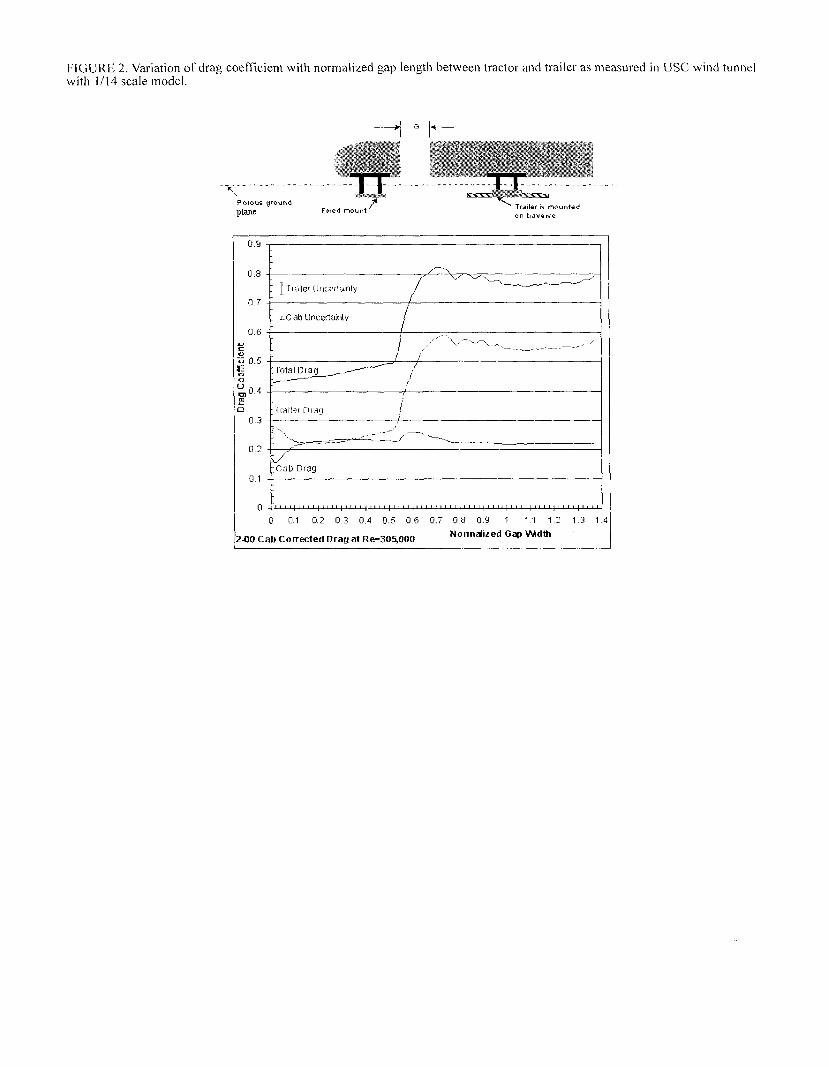
FIGURE 2. Variation of drag coeffkient with normalized gap length between tractor and trailer as measured in USC wind tunnel with 1114 scale model.

‘y‘---‘----------‘---- \

Porous ground PM=

_-____-____- _-_____-_____--__

railer k mounted on traverse

0.6 I /

i \\, .--c/-k ..)~ -- ,-' b / 2 0.5 I

ii -Total Dtag 3 :

0.3 r i I

0.1 r I

0 ""!""!""!""C"'!""!"'~!""~'~~'!~"'!""!""!""!"

0 0.1 0.: 0 3 0.4 0.5 0 6 0.7 0 8 0.9 1 II 1.2 1 3 1.‘

!XlO Cab Corrected Dray at Re=305,000 Normalized Ga(> Wdth

FIGURE 3. Streamline plots of gap flow showing two horizontal slices at mid height for two normalized gap lengths.

Hotimml tlQw slicer GIL I 65%

Spm&iC A5ymmettic

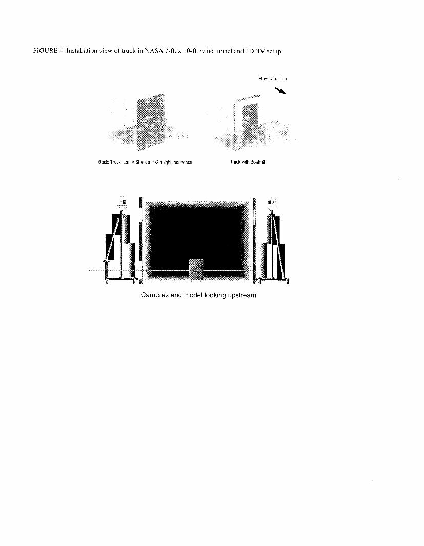
FIGURE 4. Installation view of truck in NASA 7-R. x IO-ft. wind tunnel and 3DPIV setup.

Basic Truck. Laser Sheet RI l/2 height hormntat Truck wrlh Boattatl

Cameras and model looking upstream

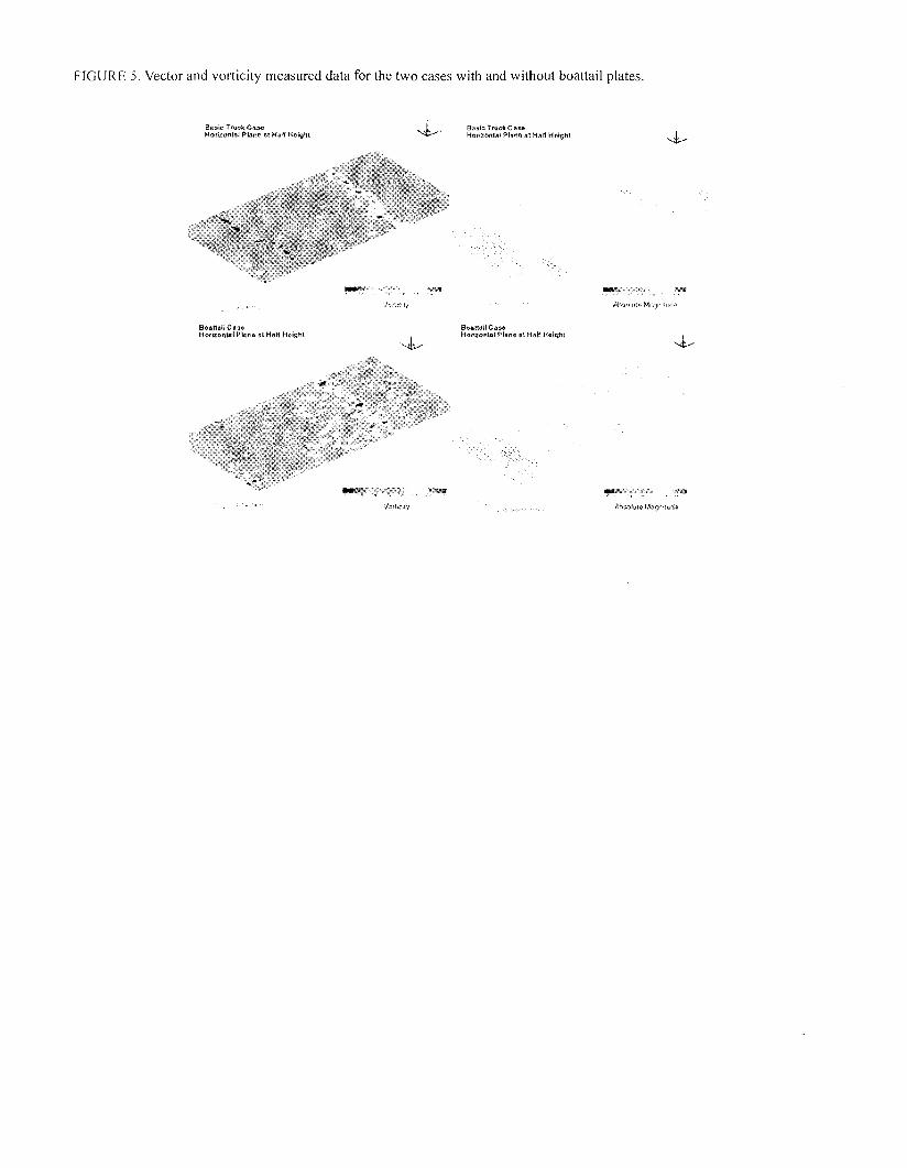
FIGURE 5. Vector and vorticity measured data for the two cases with and without boattail plates.

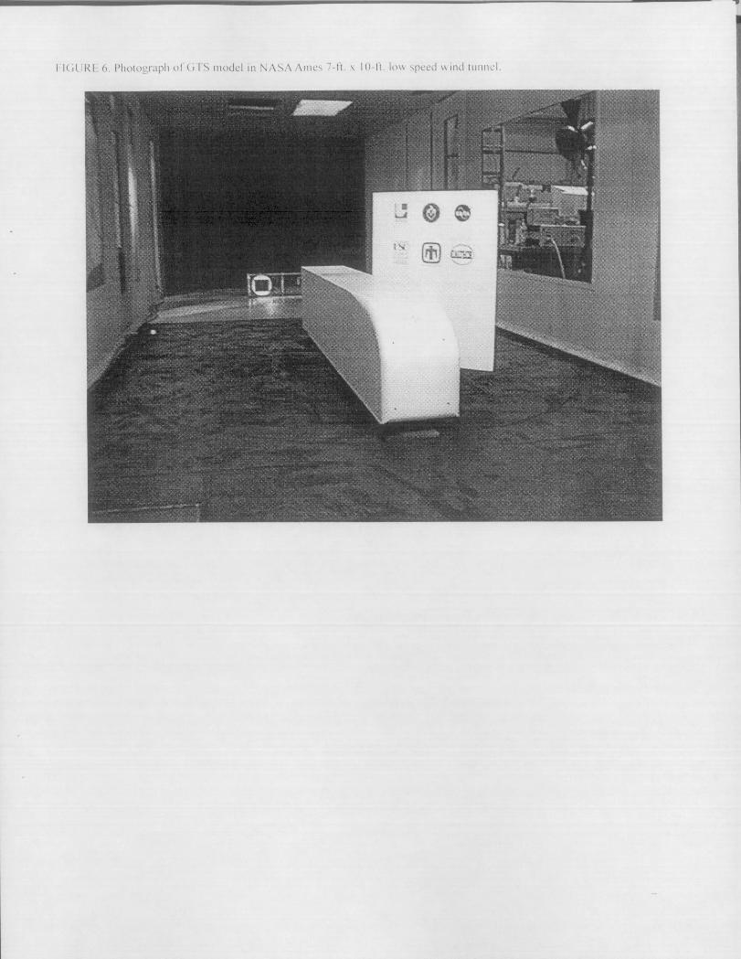
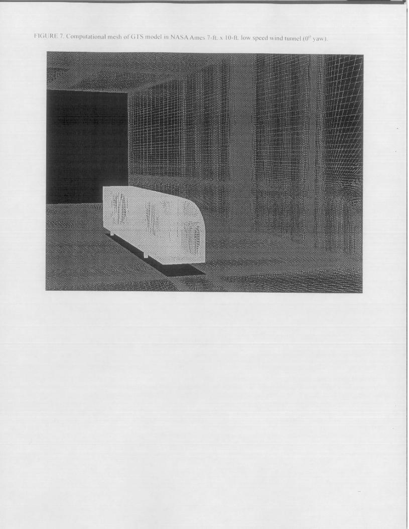
FIGURE 9. Centerline pressure distribution around GTS geometry in NASA Ames 7-ft. x IO-ft. low speed wind tunnel (0° yaw).

0

1,

_..’ -...- __..-. __ ~_,...^.-......... _...f.............._.......

. . ,.. -. I.. .o 2 ,:- .I. . . . . _

:

-0 4 “

‘

c3

-06 :

FIGURE IO. Pressure contours on GTS geometry in NASA Ames 7-ft. x IO-ft. low speed wind tunnel (0’ yaw).

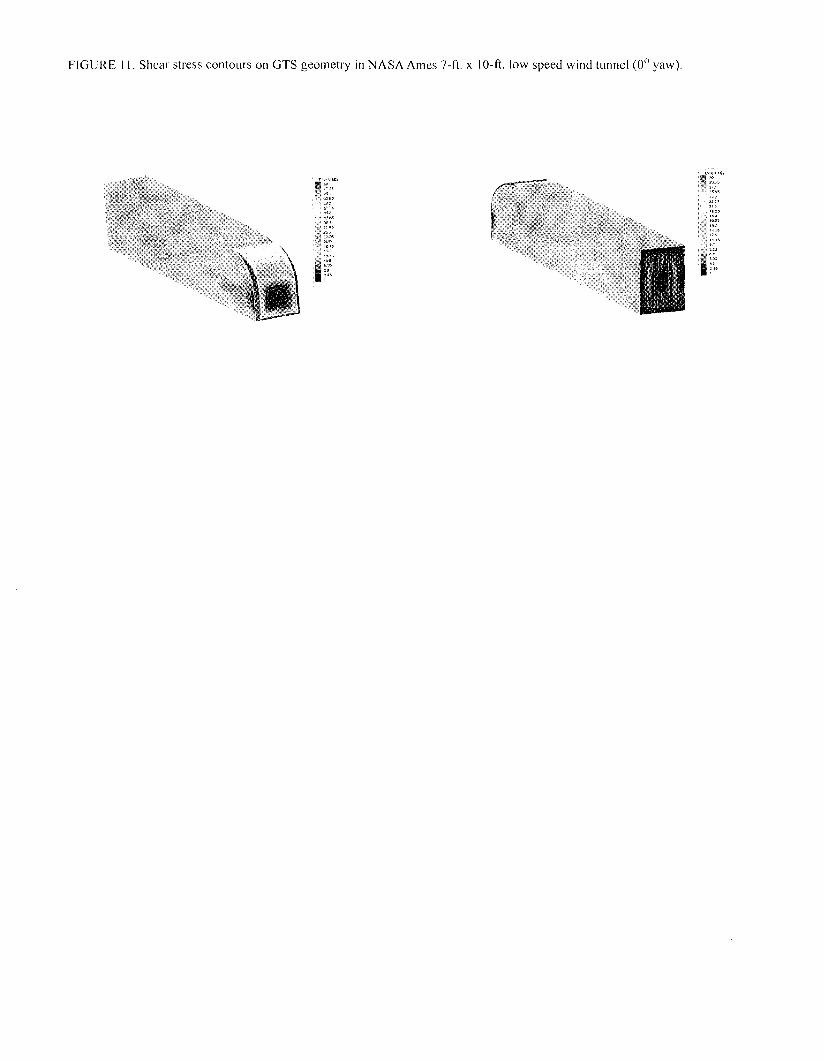
FIGURE 1 I. Shear stress contours on GTS geometry in NASA Ames 7-k x IO-ft. low speed wind tunnel (0’ yaw).

6

FIGURE 13. Pressure contours on GTS geometry in NASA Ames 7-ft. x IO-ft. low speed wind tunnel (IO’ yaw)

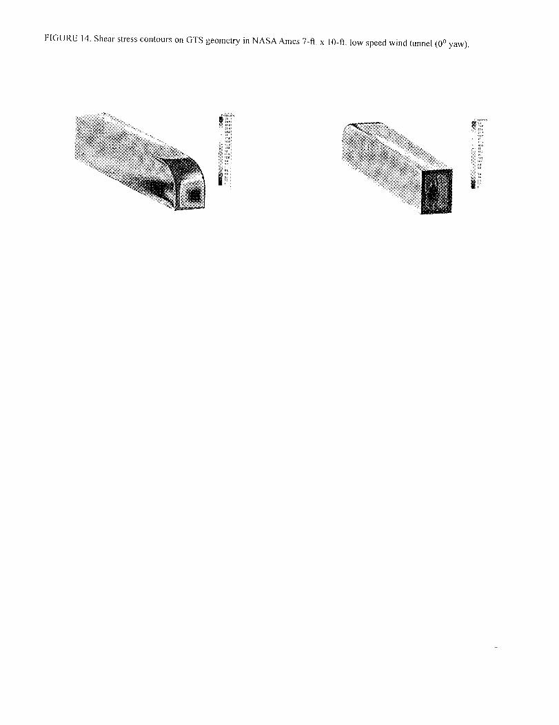
FIGURE 14. Shear stress contours on GTS geometry in NASA Ames 7-k x 10-e. low speed wind tunnel (0’ yaw)

FIGURE 15. Computational domain for LES investigation of boattails.

Compressible flow simulation Half of 3 million element grid

Domain decomposition l 148 computational domains l 148 processors on ASCI Blue

massively parallel machine (IBM)

FIGURE 16. Out-of-plane vorticity on rear of GTS with and without boattail plates.

Out-cll-pbm votticity

Em view

FIGURE 17. Starting flow around a rounded cube at Re= 100 and Ut/L=2. Results are for a slice at the body half-height.

10’ yaw

FIGURE IS. Body forces and moment versus time for IO degree yaw for rounded cube.

0.2

0

0 OS 1.5 2

0

0 0.5 1.5 2