aerodynamic drag in cycling: methods of...

Aerodynamic drag in cycling: methods of assessment

PIERRE DEBRAUX1, FREDERIC GRAPPE2, ANELIYA V. MANOLOVA1, &

WILLIAM BERTUCCI1

1LACM-DTI (EA 4302, LRC CEA 05354) UFR STAPS, Universite de Champagne-Ardenne,

Reims, France, and 2Departement de Recherche en Prevention, Innovation et Veille Technico-Sportive

(EA 4267 - 2SBP), UFR STAPS, Universite de Franche-Comte, Besancon, France

(Received 2 October 2010; accepted 25 May 2011)

AbstractWhen cycling on level ground at a speed greater than 14m/s, aerodynamic drag is the most importantresistive force. About 90% of the total mechanical power output is necessary to overcome it.Aerodynamic drag is mainly affected by the effective frontal area which is the product of the projectedfrontal area and the coefficient of drag. The effective frontal area represents the position of the cyclist onthe bicycle and the aerodynamics of the cyclist-bicycle system in this position. In order to optimiseperformance, estimation of these parameters is necessary. The aim of this study is to describe andcomment on the methods used during the last 30 years for the evaluation of the effective frontal areaand the projected frontal area in cycling, in both laboratory and actual conditions. Most of the fieldmethods are not expensive and can be realised with few materials, providing valid results in comparisonwith the reference method in aerodynamics, the wind tunnel. Finally, knowledge of these parameterscan be useful in practice or to create theoretical models of cycling performance.

Keywords: Aerodynamic drag, coefficient of drag, cycling, projected frontal area, theoretical model

Introduction

In cycling, among the total resistive forces on level ground, aerodynamic drag is the mainresistance opposed to the motion (Millet & Candau, 2002). At racing speeds greater than14m/s, with a classical racing bicycle, aerodynamic drag represents about 90% of the overallresistive forces (Candau et al., 1999; di Prampero, 2000;Martin et al., 2006;Millet &Candau,2002). Aerodynamic drag is a major concern of cycling research to enhance performance.During a cycling race (e.g. a time-trial), the time difference in performance between eliteathletes can be small. The optimisation of aerodynamic drag could be a determinant toenhance the cyclist’s performance for the samemechanical power output. In order tominimisethis resistance, it is important to know the determinant’s parameters, how to evaluate them,and what the evolution of these parameters would be as a function of the position of the cyclistand his or her displacement velocity. The purpose of this review is to present the different fieldand laboratory methods available for assessment of aerodynamic drag and its most essentialparameter, the effective frontal area, in order to enhance cycling performance.

ISSN 1476-3141 print/ISSN 1752-6116 online q 2011 Taylor & Francis

DOI: 10.1080/14763141.2011.592209

Correspondence: Pierre Debraux, UFR STAPS, Universite de Reims Champagne-Ardenne Batiment 25, Chemin des Rouliers,

Campus Moulin de la Housse, BP, 1036 – 51687, Reims Cedex, France, E-mail: [email protected]

Sports BiomechanicsSeptember 2011; 10(3): 197–218

Dow

nloa

ded

by [S

CD D

E L'

Uni

vers

ite D

e Fr

anch

e Co

mte

], [F

red

Gra

ppe]

at 0

0:14

07

Oct

ober

201

1

Characteristics of the aerodynamic drag

The major performance parameter in cycling is the displacement velocity of both cyclist andbicycle (v, in m/s). At constant velocity, the ratio of the mechanical power output generatedby the cyclist (P, in W) to the total resistive forces (RT, in N) is given by:

v ¼ P

RTð1Þ

By definition, the power output is the quantity of energy output per unit time. At constantspeed, the mechanical power output can be assumed to be the sum of the energy used toovercome the total resistive forces (De Groot et al., 1995; di Prampero, 2000). Sinceaerodynamic drag is about 90% of the total resistive forces at high speed (. 14m/s), for aconstant power output decreasing aerodynamic drag would result in an increase of thevelocity of the cyclist-bicycle system. In all forms of human-powered locomotion on land,aerodynamic drag is directly proportional to the combined projected frontal area of thecyclist and bicycle (Ap, in m2), the drag coefficient (CD, dimensionless), air density (r, inkg/m3) and the square of the velocity relative to the fluid (vf, in m/s). RD can be expressed by(e.g. di Prampero et al., 1979):

RD ¼ 0:5·ApCD·r·v2f ð2Þ

For a given velocity, aerodynamic drag is dependent on air density and the effective frontalarea (ApCD, in m2). Air density is directly proportional to the barometric pressure of the fluid(PB, in mmHg) and inversely proportional to absolute temperature (T, in K) (di Prampero,1986):

r ¼ r0·PB

760

! "·

273

T

! "ð3Þ

Where r0 ¼ 1.293 kg/m3, the air density at 760mmHg and 273K. Air density is alsoaffected by air humidity but this effect is very small and can be neglected (di Prampero,2000). Moreover, at a given temperature, the barometric pressure of fluid decreases with thealtitude above sea level (Table I). At a temperature of 273K, the decrease in barometricpressure of the fluid with altitude (Alt, in km) can be described by (di Prampero, 2000):

PB ¼ 760·e20:124·Alt ð4Þ

As seen in Table I, for the same parameters, the increase of altitude decreases aerodynamicdrag by about 24% from 0m to 2250m above the sea.

Table I. Effect of air density on aerodynamic drag

Track Alt (km) PB (mmHg) ra (kg/m3) RDb (N)

Bordeaux (France) 0 760 1.20 29.8

Colorado Springs (USA) 1.84 605 0.96 23.9Mexico City (Mexico) 2.25 575 0.91 22.6

Alt ¼ Altitude; PB ¼ Barometric Pressure; r ¼ Air density; RD ¼ Aerodynamic drag; Ap ¼ Projected frontal

area; CD ¼ Coefficient of drag; vf ¼ Velocity relative to the fluid.; aWith a temperature equal to 208C; bBased onEquation 2, for a cyclist with ApCD ¼ 0.221m2 and vf¼15m/s.

P. Debraux et al.198

Dow

nloa

ded

by [S

CD D

E L'

Uni

vers

ite D

e Fr

anch

e Co

mte

], [F

red

Gra

ppe]

at 0

0:14

07

Oct

ober

201

1

The projected frontal area

The projected frontal area represents the portion of a body which can be seen by an observerplaced exactly in front of that body, i.e. the projected surface normal to the fluiddisplacement. Some authors assume that the projected frontal area is a constant fraction ofthe body surface area to establish mathematical descriptions of aerodynamic drag (e.g.Capelli et al., 1993; di Prampero et al., 1979; Olds et al., 1993, 1995). This assumption ishelpful since the body surface area (ABSA, in m2) is easily estimated from the measurement oftwo anthropometric parameters, body height (hb, in cm) and body mass (mb, in kg) (Du Bois& Du Bois, 1916; Shuter & Aslani, 2000):

ABSA ¼ 0:00949·h0:655b ·m0:441b ð5Þ

However, Swain et al. (1987) and Garcia-Lopez et al. (2008) have shown that theprojected frontal area is not proportional to the body surface area because the ABSA/mb ratiotends to be smaller in larger cyclists. Heil (2001) reported that the assumption that theprojected frontal area and body surface area are proportional is correct for cyclists with abody mass of between 60 and 80 kg. It is generally considered that the body surface area isproportional to m0:667

b (Astrand & Rodahl, 1986), whereas the projected frontal area isproportional tom0:762

b (Heil, 2001). The projected frontal area also can be expressed with theposition of the cyclist on the bicycle from the seat tube angle (b, in degree) and the trunkangle (d, in degree) relative to the horizontal (Figure 1). The trunk is represented by the bodysegment between the hip and shoulder. A goniometer was used to measure the trunk angle:

Ap ¼ 0:00433·b0:172·d0:096·m0:762b ð6Þ

Nonetheless, Garcia-Lopez et al. (2008) observed a weak correlation between the trunkangle and the projected frontal area (r ¼ 0.42, p , 0.05). Finally, as logically expected, theresults of the different studies show that the projected frontal area is dependent on bodyheight and body mass, position on the bicycle, and equipment used (e.g. helmet, shape of the

Figure 1. Illustration of the seat tube angle (b, in degree) and the trunk angle (d, in degree) used by Heil (2001) to

determine the projected frontal area of a cyclist and bicycle, and the helmet inclination angle (a1, in degree) used byBarelle et al. (2010).

Aerodynamic drag in cycling 199

Dow

nloa

ded

by [S

CD D

E L'

Uni

vers

ite D

e Fr

anch

e Co

mte

], [F

red

Gra

ppe]

at 0

0:14

07

Oct

ober

201

1

frame, clothes). Faria et al. (2005) reported a method to determine the projected frontal areain the aerodynamic position with aero-handlebars using body height and body mass:

Ap ¼ 0:0293·h0:725b ·m0:425b þ0:0604 ð7Þ

Barelle et al. (2010) established two models to determine the projected frontal area in theaerodynamic position with aero-handlebars and a time-trial helmet, as a function of bodyheight, body mass, length of the helmet (L, in m), and its inclination on the horizontal (a1, indegree) (Figure 1):

Ap ¼ 0:107·h1:6858b þ 0:329·ðL·sina1Þ22 0:137·ðL·sina1Þ ð8Þ

Ap ¼ 0:045·h1:15b ·m0:2794b þ0:329·ðL·sina1Þ22 0:137·ðL·sina1Þ ð9Þ

However, the accessibility of direct measurement methods of the projected frontal area, asdescribed further, reduces the interest of such mathematical estimations.

The drag coefficient

The drag coefficient is used to model all the complex factors of shape, position, and air flowconditions relating to the cyclist. The drag coefficient is the ratio between aerodynamic dragand the product of dynamic pressure (q, in Pa) of moving air stream and the projected frontalarea (Pugh, 1971):

CD ¼ RD

qApð10Þ

Where the dynamic pressure is equivalent to the kinetic energy per unit of volume of amoving solid body, and defined by the equation:

q ¼ 1

2·r·v2f ð11Þ

The drag coefficient is dependent on the Reynolds number. The Reynolds number is adimensionless number that gives a measure of the ratio of inertial forces to viscous forces.Thus, the drag coefficient depends on the air velocity and the roughness of the surface. For agiven position on the bicycle, the relationship between aerodynamic drag and velocityrelative to the fluid is not linear.

In recent wind tunnel investigations, Grappe (2009) showed that the relationship betweenthe effective frontal area and the air velocity was hyperbolic (Figure 2). Measurements wereobtained on an elite cyclist with a traditional road bicycle in the traditional aerodynamicposition, where the torso is parallel to the ground, with the hands in the drop portion of thehandlebars and the elbows flexed at 908. These data indicated that the effective frontal areadecreased between 4.2 and 11.1m/s and increased between 11.1 and 27.8m/s. The lowesteffective frontal area was found between 11.1 and 13.9m/s. However, for three cyclists on atrack bicycle in the dropped position, where the torso is partially bent over with hands on thedrop portion of the handlebars and elbows fully extended, the effective frontal area decreasedbetween 5.6 and 19.4m/s (Figure 3). The position and the air velocity can have a significanteffect on the Reynolds number.


Dow

nloa

ded

by [S

CD D

E L'

Uni

vers

ite D

e Fr

anch

e Co

mte

], [F

red

Gra

ppe]

at 0

0:14

07

Oct

ober

201

1

Oggiano et al. (2009) observed, using a wind tunnel, that aerodynamic drag was alsodependent on the velocity and the roughness of the textile worn by the cyclist. Theirconclusion highlights the fact that using a rougher fabric can permit an aerodynamic dragreduction at lower displacement speeds, whereas a smoother fabric will perform better athigher speeds.Grappe (2009) also studied the effect of roughness on the effective frontal area in actual

conditions. In a velodrome, the mechanical power generated by a cyclist on a track bicyclewas measured with a SRM powermeter (Schoberer Rad Messtechnik Scientific version,Welldorf, Germany) in the traditional aerodynamic position. The power output producedby the cyclist was compared at different velocities between 8.7 and 13.9m/s in two

Figure 3. Influence of the air velocity (vf, in m/s) on the effective frontal area (ApCD, in m2) for three cyclists in staticdropped position on track bicycles, in wind tunnel. Data from Grappe (2009).

Figure 2. Influence of the air velocity (vf, in m/s) on the effective frontal area (ApCD, in m2) for one elite cyclist in

static traditional aerodynamic position on a standard road bicycle, in wind tunnel. Data from Grappe (2009).


Dow

nloa

ded

by [S

CD D

E L'

Uni

vers

ite D

e Fr

anch

e Co

mte

], [F

red

Gra

ppe]

at 0

0:14

07

Oct

ober

201

1

conditions: 1) with the cyclist-bicycle system covered with a special ’wax’ supposed toimprove the roughness and 2) without any treatment (Figure 4). Between 11 and 12m/s, nodifferencewas shownbetween the two experimental conditions. Between 8.7 and 11m/s, thesurface treatment allowed an increase in the velocity of the cyclist-bicycle system for thesame mechanical power output. However, at velocities of displacement higher than 12 m/s,the velocity did not increase when the ’wax’ was used. These results show the complexityof the relationship between the drag coefficient, air velocity, and surface roughness. Heil(2001, 2005) showed that, in cycling, the drag coefficient can be related to the body massaccording to data collected in the wind tunnel:

CD ¼ 4:45·m20:45b ð12Þ

Heil (2001) noted that the drag coefficient decreases when the body mass increases, e.g.when the body mass increases from 50 to 100 kg, the drag coefficient decreases from 0.76 to0.56. In view of the findings of Grappe (2009) on roughness and the evolution of the dragcoefficient with displacement velocity, these data have to be examined closely. Indeed, a bodymass of 100 kg corresponds to a higher body surface area than a body mass of 50 kg, thusresulting in greater skin surface area and a higher drag coefficient. Additional studies areneeded to understand the evolution of the drag coefficient as a function of cyclist parameters.

At a given velocity, the effective frontal area is the dominant component of aerodynamicdrag. In assessing the effective frontal area, it is possible to evaluate the aerodynamic profileof an athlete and to determine the optimal position on the bicycle for decreasing aero-dynamic drag. The measurement or estimation of the effective frontal area allows anevaluation of the aerodynamics of the position and equipment (Faria, 1992), which enablesthem to be optimised. It is also useful to establish mathematical models to predictperformance. Jeukendrup andMartin (2001) used a model with multiple factors concerningthe effective frontal area (e.g. body position, bicycle frame and wheels) to show the decreasein the predicted time to assess a 40 km time trial in modifying these factors.

Figure 4. Evolution of the mechanical power output (P, in W) as a function of the velocity of displacement of the

cyclist-bicycle system (v, in m/s) for a cyclist in a velodrome with a track bicycle in traditional aerodynamic position

in two conditions: 1) with the cyclist-bicycle system covered with a special ’wax’ supposed to improve the roughnessand 2) without any treatment. Data from Grappe (2009).


Dow

nloa

ded

by [S

CD D

E L'

Uni

vers

ite D

e Fr

anch

e Co

mte

], [F

red

Gra

ppe]

at 0

0:14

07

Oct

ober

201

1

Methods of assessment of aerodynamic drag

Different methods are used to evaluate aerodynamic drag under actual conditions or in thelaboratory (Garcia-Lopez et al., 2008). Once the aerodynamic drag is known, the effectivefrontal area can be computed. If the projected frontal area can be directly measured, the dragcoefficient can then be determined. Although drag coefficient is the main coefficient inevaluating the aerodynamic profile of an athlete, the validity, sensitivity and reliability of themany methods of effective frontal area and projected frontal area assessment must bediscussed. In actual situations, the projected frontal area could help to give indications about aposition in a short time with minimal equipment. With the assessment of the effective frontalarea, the measurement of the projected frontal area can be a tool to calculate a mean dragcoefficient for the most frequently used positions. With this approximation for each positiontested, coaches and cyclists could have an aerodynamic profile of a position at low cost.Results of the determination of projected frontal area and effective frontal area in the

literature, using different methods, are presented in Table II. Despite the fact that body massand height of cyclists affect the measurements, and that position on the bicycle is not alwaysclearly stated, large differences can be observed between methods for a given position. Thismay be because not all publications clearly describe the position adopted by the cyclists.Also, it is not always clear if the measurements of the projected frontal area take into accountthe projected frontal area of the bicycle. These methods of assessment are described anddiscussed in the next sections.Two ways can be used to determine the effective frontal area. On the one hand, the

aerodynamic drag can be directly measured in a wind tunnel. On the other hand, themechanical power output can be measured by a powermeter (e.g. SRM powermeterScientific version, Welldorf, Germany) at different speeds and, using Equation 1, the totalresistive force to motion is calculated in order to estimate the effective frontal area withrespect to air density.

Wind tunnel

Wind tunnels are commonly used to evaluate the effective frontal area. The wind isartificially generated from a fan on the cyclist-bicycle system, and assessment of aerodynamicdrag is based on quantification of the ground reaction forces through a plate forcemeasurement (e.g. Davies, 1980; Garcia-Lopez et al., 2008; Martin et al., 1998). In windtunnel, the cyclist is placed on the bicycle in a test position: i) motionless on a stationary plateforce; or ii) pedalling on a treadmill or on a home trainer on a plate force. Before theaerodynamic drag measurement, the force plate must be calibrated and the fan must blow amoderate wind in order to heat the wind tunnel to an optimum temperature. Theaerodynamic drag is the parallel force in the same direction as the fluid displacement. It canbe evaluated in the wind tunnel and the effective frontal area can be calculated as:

ApCD ¼ RD

0:5·r·v2fð13Þ

If this method is used in conjunction with an assessment method of the projected frontalarea, the value of the drag coefficient can be quantified. The wind tunnel is the referencetechnique to assess aerodynamic drag because of its validity and reliability (Garcia-Lopez et al.,2008; Hoerner, 1965). This technique is sensitive to wheel type (Tew & Sayers, 1999), yawangle (i.e. the angle of alignment between the bicycle and the air stream) (Martin et al., 1998),


Dow

nloa

ded

by [S

CD D

E L'

Uni

vers

ite D

e Fr

anch

e Co

mte

], [F

red

Gra

ppe]

at 0

0:14

07

Oct

ober

201

1

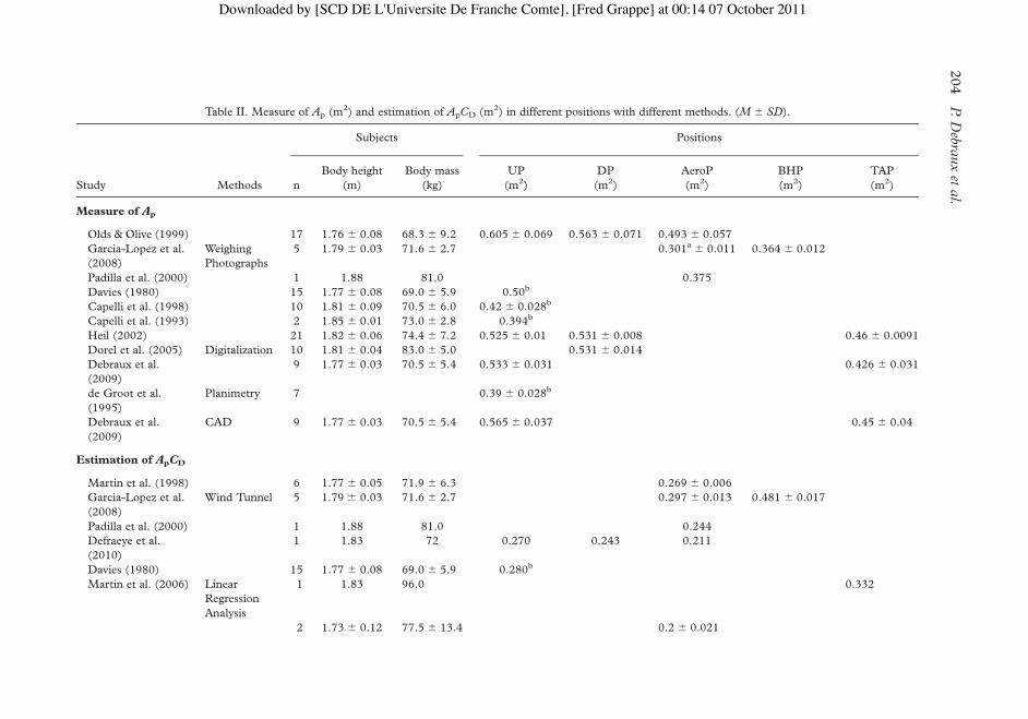
Table II. Measure of Ap (m2) and estimation of ApCD (m2) in different positions with different methods. (M ^ SD).

Subjects Positions

Study Methods n

Body height

(m)

Body mass

(kg)

UP

(m2)

DP

(m2)

AeroP

(m2)

BHP

(m2)

TAP

(m2)

Measure of Ap

Olds & Olive (1999) 17 1.76 ^ 0.08 68.3 ^ 9.2 0.605 ^ 0.069 0.563 ^ 0.071 0.493 ^ 0.057

Garcia-Lopez et al.(2008)

WeighingPhotographs

5 1.79 ^ 0.03 71.6 ^ 2.7 0.301a ^ 0.011 0.364 ^ 0.012

Padilla et al. (2000) 1 1.88 81.0 0.375

Davies (1980) 15 1.77 ^ 0.08 69.0 ^ 5.9 0.50b

Capelli et al. (1998) 10 1.81 ^ 0.09 70.5 ^ 6.0 0.42 ^ 0.028b

Capelli et al. (1993) 2 1.85 ^ 0.01 73.0 ^ 2.8 0.394b

Heil (2002) 21 1.82 ^ 0.06 74.4 ^ 7.2 0.525 ^ 0.01 0.531 ^ 0.008 0.46 ^ 0.0091

Dorel et al. (2005) Digitalization 10 1.81 ^ 0.04 83.0 ^ 5.0 0.531 ^ 0.014

Debraux et al.(2009)

9 1.77 ^ 0.03 70.5 ^ 5.4 0.533 ^ 0.031 0.426 ^ 0.031

de Groot et al.

(1995)

Planimetry 7 0.39 ^ 0.028b

Debraux et al.

(2009)

CAD 9 1.77 ^ 0.03 70.5 ^ 5.4 0.565 ^ 0.037 0.45 ^ 0.04

Estimation of ApCD

Martin et al. (1998) 6 1.77 ^ 0.05 71.9 ^ 6.3 0.269 ^ 0.006Garcia-Lopez et al.

(2008)

Wind Tunnel 5 1.79 ^ 0.03 71.6 ^ 2.7 0.297 ^ 0.013 0.481 ^ 0.017

Padilla et al. (2000) 1 1.88 81.0 0.244Defraeye et al.

(2010)

1 1.83 72 0.270 0.243 0.211

Davies (1980) 15 1.77 ^ 0.08 69.0 ^ 5.9 0.280b

Martin et al. (2006) LinearRegression

Analysis

1 1.83 96.0 0.332

2 1.73 ^ 0.12 77.5 ^ 13.4 0.2 ^ 0.021

P.Debraux

etal.

204

Downloaded by [SCD DE L'Universite De Franche Comte], [Fred Grappe] at 00:14 07 October 2011

Table II – continued

Subjects Positions

Study Methods n

Body height

(m)

Body mass

(kg)

UP

(m2)

DP

(m2)

AeroP

(m2)

BHP

(m2)

TAP

(m2)

Debraux et al.

(2009)

7 1.77 ^ 0.03 70.5 ^ 5.4 0.361c ^ 0.021

Grappe et al. (1997) 1 1.75 67.0 0.299 0.276 0.262

0.216d

Capelli et al. (1993) Towing 2 1.85 ^ 0.01 73.0 ^ 2.8 0.255a

di Prampero et al.

(1979)

2 1.75 63.0 0.318

Candau et al.(1999)

SimpleDeceleration

1 1.72 66.2 0.355 0.262-0.304

Ap ¼ Projected frontal area (m2); ApCD ¼ Effective frontal area (m2); UP ¼ Upright Position; DP ¼ Dropped Position; AeroP ¼ Aerodynamic Position withaero-handlebars; BHP ¼ Brake Hoods Position; TAP ¼ Traditional Aerodynamic Position; aWithout helmet; b Position unclear; c In mountain bike; dObree’s Position.

Aerodynam

icdrag

incycling

205

Downloaded by [SCD DE L'Universite De Franche Comte], [Fred Grappe] at 00:14 07 October 2011

and cyclist position (Garcia-Lopez et al., 2002, 2008). The results can be dependent onwhether the cyclist is motionless or moving. Indeed, during the pedalling exercise the cyclistsignificantly increases the aerodynamics. Accordingly, the plate force records the generatedforces during pedalling. To obtain a valid measurement of the drag forces, a first step could beto record the forces while pedalling in order to subtract these from the forces measured in awind tunnel.

Although the wind tunnel technique is still a reference method, it is very expensive(between 5,000 and 10,000 euros per day) and few studies have been published on theassessment of aerodynamic drag using wind tunnels. Furthermore, wind tunnelmeasurements have some limitations. Candau et al. (1999) explain that testing conditionspresent limitations: i) if the tested body does not move, the air flow around the bicycle ismodified by the floor; ii) if the wheels of the bicycle are stationary, the effect of wind is notmeasured; and, iii) the cyclist’s position on the bicycle during the tests is not necessarilyidentical to the position in actual conditions. Slight lateral movements that can occur inactual conditions are not present in the wind tunnel. When the cyclist rides on a motor-driven treadmill or a home trainer, limitations ii and iii are resolved, but another limitationsappears: iv) the pedalling motion introduces noises in the force measurement system suchthat there are changes in the forces applied to the treadmill within each pedal revolution; and,v) slight lateral movements (e.g. shoulders) are dependent of the intensity of pedalling.

Few studies have simulated actual conditions of pedalling in a wind tunnel. In Davies’study (1980), the cyclists were instructed to pedal on a motor-driven treadmill at a set speedof 4.7m/s against wind velocities varying from 1.5-18.5m/s. To be closer to ridingconditions, Martin et al. (1998) simulated pedalling at 90 rotations per minute (rpm), butwithout resistance, and the front wheel was rotated by a small electric motor. Garcial-Lopezet al. (2002, 2008) tested five different positions to measure the aerodynamic drag ofprofessional cyclists in a wind tunnel using two bicycles, a special time-trial bike with aero-handlebars and a standard bike with standard handlebars. These tests occurred with andwithout pedalling against a resistance ergometer.

In order to model actual conditions more closely, it could be more practical to use a fieldmethod to assess the effective frontal area. This permits lower cost testing in actualconditions and enables selection of the most appropriate position and equipment.

Method of linear regression analysis

When cycling on level ground at constant velocity, the total resistive forces are mainlycomposed of two forces, aerodynamic drag and rolling resistance (RR, in N). Thus, the totalresistive forces can be described by Equation 14 (Capelli et al., 1993; Davies, 1980; diPrampero et al., 1979; Grappe et al., 1997, 1999):

RT ¼ RDþRR ð14Þ

With

RR ¼ CR·M·g ð15Þ

Rolling resistance represents the contact forces between the ground and the pneumatics ofthe wheels, and the frictional losses at the bearing and transmission chain (Grappe et al.,1997; Millet & Candau, 2002). Rolling resistance depends on the rolling coefficient (CR,dimensionless), the mass of the cyclist-bicycle system (M, in kg) and the gravity acceleration


Dow

nloa

ded

by [S

CD D

E L'

Uni

vers

ite D

e Fr

anch

e Co

mte

], [F

red

Gra

ppe]

at 0

0:14

07

Oct

ober

201

1

(g ¼ 9.81m/s2). According to Equations 2, 14 and 15:

RT ¼ 0:5·rApCD·v2f þCR·M·g ð16Þ

The total resistive forces can be determined by measuring mechanical power output as afunction of velocity (Grappe et al., 1997):

RT ¼ P

vð17Þ

This method consists of measuring mechanical power output using a powermeter (e.g.SRM powermeter Scientific version, Welldorf, Germany) at different velocity to determinethe total resistive forces. To do this, the cyclist performs several trials at different velocities ina selected posture. According to Equation 16:

a ¼ 0:5·r·ApCD ð18Þ

b ¼ CR·M·g ð19Þ

Thus

RT ¼ av2þb ð20Þ

Based on Equation 20, the total resistive forces vary in a linear way with the square of thevelocity (Figure 5).With a linear regression analysis, it is possible to determine the effective frontal area value

for the selected posture according to Equation 18 (ApCD ¼ a/0.5r) from the slope a ofEquation 20. If this method is used with a method of determination of the projected frontalarea, the value of the drag coefficient can be quantified (Capelli et al., 1998). However, therelationship between the total resistive forces and v 2 is not necessarily linear (Grappe, 2009).

Figure 5. Illustration of the evolution of the total resistive forces (RT, in N) as a function of the squared displacementvelocity of the cyclist-bicycle system (v2, in m2/s2) on level ground with a mountain bike.


Dow

nloa

ded

by [S

CD D

E L'

Uni

vers

ite D

e Fr

anch

e Co

mte

], [F

red

Gra

ppe]

at 0

0:14

07

Oct

ober

201

1

The reliability of this method is good (Coefficient of variation (CV) ¼ 3.2%) (Grappeet al., 1997). Grappe et al. (1997) did not observe a significant difference, using theMax Onepowermeter (Look SA, France), between the aerodynamic position with aero-handlebars,where the lower arms are on the aerodynamic handlebars, and the dropped position. Thedifference in the effective frontal area between the two positions was 4.6%, and the authorsconcluded that this method reaches the limit of the sensitivity of the measurement. Thepowermeter used (Max One, Look SA, Nevers, France) to measure the mechanical poweroutput has a weak sampling frequency (i.e. 4 data per 1 rpm) and the tests were performed inan outdoor velodrome. The use of a more accurate powermeter like the SRM, which has ahigher sampling frequency, could lead to a more sensitive measure in the field. It could behelpful in discriminating different positions or levels of roughness.

To verify whether the SRM system could provide a valid measure of cycling power, Martinet al. (1998) compared the SRM measured power with that from the Monark cycleergometer (Model 818). The statistically valid results indicate that the power measured bythe SRM was significantly different ( p , 0.01) than the power delivered to the Monarkergometer flywheel; the difference was 2.35%. It appears that this difference is characteristicof power loss in chain drive systems (Martin et al., 1998). These authors assume that theSRM provides a valid and accurate measure of cycling power compared with the Monarkcycle ergometer.

Measurement of the tractional resistance (dynamometric method): the ’towing’ method

With this method, tractional resistance is determined by towing a subject with a vehicle (e.g.car, motorcycle) by means of a cable (e.g. a nylon cable of 0.003m of diameter) on a flattrack at constant speed. The length of the cable (e.g. 10m, 25m) was chosen to minimise theair turbulence caused by the moving vehicle (di Prampero et al., 1979; Capelli et al., 1993).However, air turbulence set up by the towing vehicle and alterations in atmosphericconditions can affect the results (Candau et al., 1999; Garcia-Lopez et al., 2008). During thetest, the cyclist’s selected posture does not change while being towed by the vehicle. Thecyclist can pedal at a selected cadence without a transmission chain to reproduce the airturbulence induced by moving legs during actual cycling (Capelli et al., 1993).

The total resistive forces to the motion were measured with a dynamometric techniquefrom a load cell mounted in series on the cable. The total resistive forces were assessed overseveral trials at different velocities to obtain a RT-v relationship. As for the method of linearregression analysis, the curve of the total resistive forces in function of the square of thevelocity has to be plotted, based on Equation 20. With a linear regression analysis, it ispossible to determine the effective frontal area value for the studied position according toEquation 16 (ApCD ¼ a/0.5r) from the slope a of Equation 20. Capelli et al. (1993) testedthe repeatability of the towing method by measuring the total resistive forces twice each at sixspeeds. They found no significant difference between the paired sets of data (p . 0.10). Thefact that this method cannot be used routinely is an important limitation.

The coasting-down and deceleration methods

These methods of measuring aerodynamic drag are based on Newton’s second law(SF ¼ m·a), where the sum of the resistive forces (F) is equal to the product of mass (m) withacceleration (a). The tests performed in descent (coasting-down method) measure theacceleration of the cyclist in free-wheel and those performed on flat terrain (outdoor andindoor) measure the cyclist’s deceleration, also in free-wheel. In a specified position i) in a


Dow

nloa

ded

by [S

CD D

E L'

Uni

vers

ite D

e Fr

anch

e Co

mte

], [F

red

Gra

ppe]

at 0

0:14

07

Oct

ober

201

1

descent (Gross et al., 1983; Kyle & Burke, 1984; Nevill et al., 2006) or ii) on flat ground, in afield, or in hallways (Candau et al., 1999) the cyclists brought the bicycle to a defined velocitybefore they stopped pedalling. The riding position was unchanged and, to reproduce actualconditions with turbulence induced by movement of the lower limbs, the cyclists can pedalwithout transmission of force to the rear wheel during coasting trials (Gross et al., 1983;Kyle &Burke, 1984; Candau et al., 1999). In this way, the cyclists slowed down due to the air frictionand rolling resistive forces over several timing switches.For the coasting-downmethod (Gross et al., 1983; Kyle & Burke, 1984), there are six timing

switches. The distance between switches is 6 metres and the time is recorded using achronometer system (to 1/1,000 s). The mean velocity between each switch is calculated toassess linear regression of mean velocity as a function of the distance. The slope of the linearregressionmultipliedby themeanvelocityof the third interval determines themean accelerationof the bicycle-cyclist system. The total resistive forces are the product of the mass and theacceleration of this system.The aerodynamic drag and the rolling resistance are calculated fromthe relation between the total resistive forces and the square velocity as shown in Equation 16.As the coasting-down method is a field method, climatic conditions and the nature of the

ground can potentially induce some errors. Kyle and Burke (1984) reported measuredvariations of nearly 10%. To avoid such errors, the method can be used in hallways (DeGroot et al., 1995). De Groot et al. (1995) have developed a small infrared light emitter anddetector mounted on the front fork of the bicycle. This system can measure velocity as afunction of time during the deceleration phase but there is no information concerning thereliability and sensitivity of this approach.For the deceleration method (Candau et al., 1999), three switches are disposed in a

hallway. The distance between the first and the second switch is 3 metres and the distancebetween the second and third switch is 20 metres (Figure 6).The time is recorded using a chronometer system (accurate to 30ms). The total resistive

forces were assessed with several trials (< 20) at different velocities by iterations with amathematical model describing the deceleration of the trajectory of the cyclist-bicycle system(Candau et al., 1999). The reliability (CV ¼ 0.6%), sensitivity and validity of this method ofmeasuring the effective frontal area (in comparison with the wind tunnel) are excellent.Although this method permits measurement of the rolling resistance of the tyres according toa specific ground surface, it is limited by the significant number of trials needed to determinean evaluation of the effective frontal area.Of these four methods of assessment of the effective frontal area, the wind tunnel method

and the method of linear regression analysis are the most sensitive and reliable. The method

Figure 6. Schematic view of the measurement system for the deceleration method in a hallway and the placement ofthe three switches.


Dow

nloa

ded

by [S

CD D

E L'

Uni

vers

ite D

e Fr

anch

e Co

mte

], [F

red

Gra

ppe]

at 0

0:14

07

Oct

ober

201

1

of linear regression analysis with the use of a powermeter such as SRM providesmeasurement of the resistive forces in actual conditions. It could also help to discriminatebetween the effective frontal area values at different positions. However, the wind tunnelallows more accurate and reliable measurements of aerodynamic drag, resulting in a highersensitivity to small adjustments of the cyclist’s position (Defraeye et al., 2010) or equipment(e.g. the helmet) (Barelle et al., 2010). Nevertheless, this method is very expensive. Mostcoaches and sport scientists have easier access to a powermeter system like the SRM orPowerTap models. The field method could serve to prepare and/or optimise and/or verifywind tunnel results. Finally, Defraeye et al. (2010) showed that computational fluiddynamics provided measurements of drag in good agreement with those obtained by windtunnel tests. Computational fluid dynamics could be a valuable numerical alternative forevaluating the drag of different cyclist positions with high sensitivity. The advantage of thismethod is that it allowsmore detailed insight into the flow field around the body of the cyclist.

Although the effective frontal area is the main parameter in aerodynamic evaluation, it canbe highly influenced by the projected frontal area. For a constant drag coefficient, the effectivefrontal area is proportionally affected by the change of projected frontal area. Moreover, adecrease in the projected frontal area would result in a decrease in the effective frontal area(Defraeye et al., 2010). Two different methods are used to measure the projected frontalarea: i) with a calibration frame of known area, such as the method of weighing photographs(e.g. Capelli et al., 1993, 1998; Debraux et al., 2009; di Prampero et al., 1979; Heil, 2001;Olds et al., 1993, 1995; Padilla et al., 2000; Pugh, 1970, 1971; Swain et al., 1987), themethod of digitalisation (Barelle et al., 2010; Debraux et al., 2009; Dorel et al., 2005; Heil,2001, 2002)); and ii) without calibration frame, such as planimetry (Olds & Olive, 1999),digital methods using computer-aided design (CAD) software (Debraux et al., 2009)).

The method of weighing photographs

This method consists of taking a photograph in a frontal plane of the cyclist and bicycle(Figure 7A). A calibration frame with a known area located midway between the subject’ship and shoulders and facing the camera is also photographed. The photograph is printedand the cyclist and calibration frame are cut from the photograph. These separate pieces areweighed using an accurate balance with a high sensitivity (^0.001 g). The actual projected

Figure 7. Example of photographs of cyclists used to measure Ap with different methods: method of weighingphotographs (A), method of digitalisation (B), and computer-aided design method (C).


Dow

nloa

ded

by [S

CD D

E L'

Uni

vers

ite D

e Fr

anch

e Co

mte

], [F

red

Gra

ppe]

at 0

0:14

07

Oct

ober

201

1

frontal area in square metres is calculated for each image by multiplying the known area ofthe calibration frame by the ratio of the projected frontal area image weight over thecalibration frame image weight (Capelli et al., 1998; Debraux et al., 2009; Heil, 2001;Olds et al., 1995; Padilla et al., 2000).The method of weighing photographs requires only a calibration frame, a digital camera, a

balance with high sensitivity, and a cutting instrument, but it cannot be used in actualconditions because of the need of the calibration frame. Although this method has been usedfor a long time (Pugh, 1970, 1971; Swain et al., 1987), it is very reliable (CV ¼ 1.3%)(Debraux et al., 2009) and has been used to test the validity of new methods of assessment ofthe projected frontal area (e.g. Debraux et al., 2009; Heil, 2001).The method of weighing photographs presents some inconvenience which can be resolved.

The cutting of the printed photograph following the outline of the cyclist has to be veryaccurate, and this operation takes at least 5–6 minutes. Moreover, for the classical format ofdigital photographs, it is easier to measure only the projected frontal area of the cyclistwithout the bicycle, unless the photographs are enlarged. To be sure that colour did notinfluence the mass of photographs, Debraux et al. (2009) weighed five photographs with fivedifferent colours. They concluded that colour did not influence the results in this method.

Planimetry

In planimetry, the outline of the cyclist and bicycle is traced with a polar planimeter, and atriangulation method is used to calculate the enclosed area (Olds & Olive, 1999). Olds andOlive (1999) compared a method based on weighing pictures and planimetry whilemeasuring Ap cyclist in three positions: i) Upright position: where the torso is upright with thehands placed near the stem of the handlebars; ii) Dropped position: partially bent over torsoposition with hands on the drop portion of the handlebars and elbows fully extended; andiii) Aerodynamic position: where the arms are resting on aero-handlebars. The authorsobserved a significant mean difference (, 3.3%) between the projected frontal areasdetermined by the two methods. Both methods were extremely reliable but weighingphotographs gave a more precise result than the planimetry-based method. The meandifferences were 0.25% vs. 2.90% respectively for the weighing photographs and planimetry.

Digitalisation

Like the method of weighing photographs, the digitising method (Barelle et al., 2010;Debraux et al., 2009; Dorel et al., 2005; Heil, 2001, 2002) requires the use of a calibrationframe with a known area placed near the cyclist and bicycle. However, this digital methoddoes not require the cutting of photographs; instead, it consists of digitalising a paper picturewith the help of a digitiser (Heil, 2001), or with a computer-based image analysis softwareapplication (e.g. Scion Image Release Alpha 4.0.3.0.2 for Windows, Scion Corporation,Frederick, Md., USA or ImageJ software) if the pictures are in numerical format (Barelleet al., 2010; Debraux et al., 2009; Dorel et al., 2005; Heil, 2002). Accurate preparation isneeded in order to be able to use numerical pictures. The zones to be measured must bedarkened. This can be done in two ways, either by converting the picture into a black andwhite file using computer-based imaging software (e.g. Gimp, Adobe Photoshop) (Debrauxet al., 2009) or by using a light placed behind the cyclist and bicycle (Dorel et al., 2005).In a computer-based image analysis software application (e.g. Scion Image Release Alpha

4.0.3.0.2 for Windows, Scion Corporation, Frederick, Md., USA), the black and whiteimage is imported, and the zones of the cyclist with the bicycle and the calibration frame are


Dow

nloa

ded

by [S

CD D

E L'

Uni

vers

ite D

e Fr

anch

e Co

mte

], [F

red

Gra

ppe]

at 0

0:14

07

Oct

ober

201

1

selected (see Figure 7B). The software measures the number of pixels included in the zones.The actual projected frontal area in square metres of the digitised image is obtained bydetermining the ratio of pixels of the two zones then multiplying this ratio by the actualknown area of the calibration frame. To measure only the cyclist projected frontal area, it isnecessary to take a picture of the cyclist and bicycle, and one of the bicycle alone, thenmanually subtract the pixel count from the picture of the bicycle alone from the pixel countof the picture representing both cyclist and bicycle.

The digitising method needs a personal computer (but the software is free and easy to use)and a digital camera or a scanner to digitise the printed photographs. However, it requiresthe investigator to correct the photographs (e.g. darken the measured zone, change theextension of the image file) before opening them in the software Scion Image, which will taketime and practice. This method is valid in comparison with the method of weighingphotographs (Heil, 2001; Debraux et al., 2009).

Method based on computer-aided design (CAD) software

The methods based on CAD software do not require a calibration zone to be placed near thecyclist and can be used in actual conditions. The calibration is assessed by entering a knowndistance (vertical or horizontal) corresponding to a distance in the photographs (e.g. thewidth of the handlebars, the height of the front wheel) in the software (Figure 7C). The digitalphotographs are opened in CAD software. The outlines of the area measured are traced witha spline curve tool in a 2D plane. The software calculates the area enclosed (Debraux et al.,2009). This method is valid in comparison with the method of weighing photographs andreliable (CV ¼ 0.1%) (Debraux et al., 2009). It is a fast method, but it needs a personalcomputer andCAD software, which are both relatively expensive. As this method can be usedin actual conditions, it is possible to test the aerodynamic drag of different positions at a lowercost by using it together with linear regression analysis or towing.

Among the different methods described to assess the projected frontal area, thedigitalisation method and the methods based on a CAD software are better adapted for thedigital image format. Planimetry and the method of weighing photographs both require moreprocedures and more time for a measurement which could be done in five minutes utilisingthe new digital methods (Debraux et al., 2009). However, all these methods are reliable, andthere is no significant difference between weighing photographs, digitalisation, and themethod based on CAD software (Heil, 2001; Debraux et al., 2009). The new methods aresimply faster and more convenient.

Nevertheless, all these methods have in common the need to take a photograph of thecyclist-bicycle system. Since the measurement of the projected frontal area is dependent onthe photograph, the placement of the calibration frame and the optical calibration of thedigital camera can be source of errors. To study these measurement errors, Olds and Olive(1999) determined the effects on the projected frontal area of the calibration frame positionand the position of the camera relative to the cyclist-bicycle system. The authors made somerecommendations in order to standardise the measurement protocol of the projected frontalarea using a calibration frame, or not: i) The frontal plane of the calibration frame has to belocated approximately midway between the cyclist’s hip and shoulder. Olds and Olive (1999)showed that when the calibration frame was moved back to the rear wheel-tip, the projectedfrontal area increased by 61%, and when it was placed at the front wheel-tip, the projectedfrontal area decreased by 46%; ii) The digital camera has to be directed straight towardsthe cyclist at the height of the handlebars in the axis of the bicycle. An angular deviation of108of the digital camera could induce a 7.5% increase of the projected frontal area measure


Dow

nloa

ded

by [S

CD D

E L'

Uni

vers

ite D

e Fr

anch

e Co

mte

], [F

red

Gra

ppe]

at 0

0:14

07

Oct

ober

201

1

(Olds & Olive, 1999); and iii) The digital camera has to be located at least 5 metres awayfrom the cyclist-bicycle system. This is to minimise distortion due to focal length and thedifferences in apparent size of the parts of the cyclist closer and further from the digitalcamera (Olds & Olive, 1999).

How to minimise aerodynamic drag

In cycling, aerodynamic drag is composed of two forms of drag: pressure and skin-frictiondrag (Faria, 1992; Millet & Candau, 2002). Pressure drag is the most important part ofaerodynamic drag. It represents the difference of air pressure that exists between the frontand rear of a moving body. Within a fluid, a moving body creates a boundary layer due to thefluid pressure on the body and leads to backward turbulence resulting in pressure drag.Pressure drag is mainly dependent on the general size and shape of the body. Skin-frictiondrag is the resistance generated by the friction of fluid molecules directly on the surface of thebody in motion. It increases with the size and roughness of the body surface (Millet &Candau, 2002).As explained previously, the effective frontal area is the determinant parameter of the

cyclist-bicycle system aerodynamic. Both general size and shape of the moving body affectthe effective frontal area, and can be decreased in different ways according to Kyle and Burke(1984) andMillet and Candau (2002). A cyclist can lower aerodynamic drag in reducing theprojected frontal area. The angle between the trunk and the ground is important, the nearerthe angle to 0 degrees, the more the projected frontal area decreases (Heil, 2001). Faria(1992) reported a decrease of 20% of the aerodynamic drag when the cyclist’s elbows arebent with the torso nearly parallel to the ground. The position of the arms is a supplementaryfactor to modify in order to enhance the projected frontal area. A decrease of 28% inaerodynamic drag was observed when the hands were on the centre of the upper handlebars,trunk resting on the hands, crank parallel to the ground (Faria, 1992). The hands can beplaced forwards in relation to the body in using aero-handlebars, and this can increasecomfort and decrease the projected frontal area. Moreover, Berry et al. (1994) did not findsignificant differences between aero-handlebars and standard racing handlebars in terms ofexhaustion, power output and oxygen consumption.The effects of the moving cyclist-bicycle system shape on the aerodynamic drag are

quantified by the drag coefficient (di Prampero, 1986). To reduce the drag coefficient, theshape of the moving body has to be streamlined. The position, an aerodynamic bicycleframe, aerodynamic helmet, aerodynamic wheels (Tew & Sayers, 1999), and clothes andaccessories can significantly reduce the drag coefficient (Faria, 1992; Faria et al., 2005). Tewand Sayers (1999) showed that aerodynamic wheels could reduce the axial drag of up to 50%in comparison with the spoked wheels. Different techniques exist to enhance the effectivefrontal area for the cyclist-bicycle system, and every improvement must be tested andquantified to find out whether the decrease in effective frontal area can save significant time inactual racing conditions (e.g. time-trials) (Atkinson et al., 2007). This is why mathematicalmodels of cycling performance are necessary to simulate mechanical power output, whichdepends on many parameters.

Importance of the effective frontal area in modelling cycling performance

A theoretical model can provide a helpful simulation tool for researchers, coaches, andcyclists who do not have access to the technologies indicated above (e.g. powermeter,computer). Indeed, a model permits the effect on cycling performance of physiological


Dow

nloa

ded

by [S

CD D

E L'

Uni

vers

ite D

e Fr

anch

e Co

mte

], [F

red

Gra

ppe]

at 0

0:14

07

Oct

ober

201

1

changes, biomechanical, anthropometric, and environmental factors to be predicted (Oldset al., 1993). Many authors have established a mathematical cycling model (e.g. Atkinsonet al., 2007; Broker et al., 1999; di Prampero et al., 1979; Heil et al., 2001; Martin et al.,2006; Nevill et al., 2006; Olds, 1998, 2001; Olds et al., 1993, 1995; Padilla et al., 2000),most including terms for power output produced by the cyclist and power required toovercome aerodynamic drag, rolling resistance, and other parameters (Martin et al., 2006).At displacement velocity greater than 14m/s where the aerodynamic drag is about 90% of thetotal resistive forces, according to Equations 1 and 2, it can be assumed that the mechanicalpower output is proportional to the product of aerodynamic drag and velocity. Themechanical power necessary to drive the cyclist-bicycle system through the air will increasewith the cube of the velocity (Faria, 1992).

Gonzales-Haroet al. (2007)and(2008)havecomparednine theoreticalmodels for estimatingthe power output in cycling using the SRM powermeter in a velodrome. The most importantvariables in these models are: velocity, mass of the cyclist-bicycle system, and aerodynamicvariables: the projected frontal area and the drag coefficient. Other secondary variables are theslope, rolling coefficient and climatic conditions (barometric pressure of the fluid andtemperature).Gonzales-Haro et al. (2007) found the equations of di Prampero et al. (1979) andCandau et al. (1999) the best estimates of power output in comparisonwithmeasurementswiththe SRM powermeter, whereas Gonzales-Haro et al. (2008) found the equation of Olds et al.(1995) best to estimate peak power output because of the few variables to measure.

As on level ground, at racing speeds greater than 14m/s, aerodynamic drag representsabout 90% of the overall resistive forces (Candau et al., 1999; di Prampero, 2000; Martinet al., 2006; Millet & Candau, 2002) and consideration of the effective frontal area in amathematical model is important. Its estimation can strongly influence the model. However,some simulations did not take it in account or are based on approximation (Table III).

Olds et al. (1995) established a relationship between the projected frontal area and thebody surface area considering that the projected frontal area is a constant fraction of the bodysurface area in a given position:

Ap ¼ 0:3176·ABSA20:1478 ð21Þ

These equations do not take into account the differences intra- and inter-individual for thesame position on the bicycle, or different bicycles. In these authors’ model, the dragcoefficient was a constant and equal to 0.592. For comparison, we estimate the projectedfrontal area according to Olds et al. (1995) and we measure the projected frontal area usingthe CAD method (Debraux et al., 2009). The revisited equation of the body surface area byShuter and Aslani (2000) was used (see Equation 5), where the body surface area is expressedin square metres but the body height is expressed in cm. Table IV presents the results of thedifference between the two methods on seven cyclists in traditional aerodynamic position.The mean results show an increase of 0,021m2 (þ4.9%) for the projected frontal area withthe method of Olds et al. (1995). The twomethods are compared with a paired t-test and thedifference is significant ( p , 0.05). However, additional studies should be performed on theaccuracy of the methods for the projected frontal area determination.

In order to be valid, the mathematical model for an estimation of the projected frontal areamust consider various parameters (e.g. the position of the cyclist, the wearing of a helmet). Inthis way, the drag coefficient that changes with position and velocity has to be determined.Martin et al. (2006) found that the effective frontal area values determined in field trials withthe SRMpowermeter were similar to those measured in the wind tunnel. This method is veryuseful to assess the effective frontal area in actual conditions as routine and the cyclists can


Dow

nloa

ded

by [S

CD D

E L'

Uni

vers

ite D

e Fr

anch

e Co

mte

], [F

red

Gra

ppe]

at 0

0:14

07

Oct

ober

201

1

Table IV. Comparison of the estimation of Ap with the equation developed by Olds et al. (1995) using ABSA

calculated according Shuter and Aslani (2000) and the measure of Ap with the CADmethod (Debraux et al., 2009)for cyclists in traditional aerodynamic position with modern bicycle

Subjects hb (m) mb (kg) Ap (m2) Olds et al. (1995) Ap (m2) Debraux et al. (2009)

Subject 1 1.74 78 0.456 0.406Subject 2 1.81 70 0.443 0.425

Subject 3 1.90 75 0.481 0.424

Subject 4 1.85 72 0.459 0.425

Subject 5 1.70 64 0.397 0.385Subject 6 1.80 64 0.417 0.416

Subject 7 1.75 65 0.412 0.401

Subject 8 1.80 75 0.459 0.461Subject 9 1.75 91 0.501 0.488

M ^ SD 1.79 ^ 0.06 72.7 ^ 8.6 0.447* ^ 0.034 0.426* ^ 0.031

*Significant difference at p , 0.05Ap ¼ Projected frontal area (m2); ABSA ¼ Body surface area (m2); hb ¼ Body height (m); mb ¼ Body mass (kg).

Table III. Mathematical expression of the aerodynamic parameters in modelling of the power output

Study Method of calculation of the aerodynamic parameters

Whitt (1971) Ap has to be determineddi Prampero et al. (1979) Based on a percentage of ABSA with ABSA ¼ 0:007184·m0:425

b ·h0:725b

Kyle (1991) CD ¼ 0.8

Ap has to be determined

Menard (1992) SCx ¼ 0.259m2

SCxv ¼ 0.012m2

Olds et al. (1993) Based on a percentage of ABSA ABSA ¼ 0:007184·m0:425b ·h0:725b

CFA ¼ ABSA / 1.77

Broker (1994) K1 ¼ Kd·Kpo·Kb·Kc·Kh

Ap has to be determined

Olds et al. (1995) CD ¼ 0.592

Ab ¼ 0:3176·ABSA20:1478TotalAp ¼ 0:4147·ðAb=1:771Þþ0:1159

Candau et al. (1999) ApCD ¼ 0.333m2

Shuter and Aslani (2000) ABSAðm2Þ ¼ 0:00949·h0:655b ·m0:441b with hb in cm

Heil (2001) Ap ¼ 0:00433·STA0:172·TA0:096·m0:762b

CD ¼ 4:45·m20:45b

Faria et al. (2005) FA ¼ 0:0293·h0:725b ·m0:425b þ0:0604

Martin et al. (2006) ApCD has to be determined

Barelle et al. (2010) Ap ¼ 0:107·h1:6858b þð0:329 ðL·sina1Þ220:137·ðL·sina1ÞÞAp ¼ 0:045·h1:15b ·m0:2794

b þð0:329 ðL·sina1Þ220:137·ðL·sina1ÞÞ

Ap ¼ Projected frontal area (m2); Ab ¼ Projected frontal area of the body (m2); ABSA ¼ Body surface area (m2);

mb ¼ Body mass (kg); hb ¼ Body height (m); CD ¼ Coefficient of drag; SCx ¼ Coefficient of air penetrationdetermined in wind tunnel (m2); SCxv ¼ Wheel’s coefficient of air penetration determined in wind tunnel (m2);

CFA ¼ Correction factor for body surface area (m2); K1 ¼ Aerodynamic factor; Kd ¼ Air density; Kpo ¼ Rider

position; Kb ¼ Cycle components; Kc ¼ Clothing; Kh ¼ Handlebar type; FA ¼ The total frontal area of thecyclist in the aerodynamic position with Aero-Handlebars (m2); L ¼ Length of a time-trial helmet (m); a1 ¼Helmet inclination on the horizontal (degree).


Dow

nloa

ded

by [S

CD D

E L'

Uni

vers

ite D

e Fr

anch

e Co

mte

], [F

red

Gra

ppe]

at 0

0:14

07

Oct

ober

201

1

test several positions and bicycles. Considering the mathematical model of Olds et al. (1995)as the best estimate of the peak power output (Gonzales-Haro et al., 2008), it could be moreappropriate to use this model with the effective frontal area estimated by the method of linearregression analysis.

Conclusion

The effective frontal area is the most important parameter to characterise aerodynamic drag.The techniques of estimation of the effective frontal area are now well recognised in cycling,and this parameter can be reliably evaluated in laboratory or actual conditions. However,although the projected frontal area is a well-known easily quantifiable factor, the variation ofthe drag coefficient is more complex. Its evolution as a function of velocity is still difficult tounderstand fully. More research will be necessary to study the characteristics of dragcoefficient variation. New methods such as computational fluid dynamics could be a greathelp in achieving this. Knowledge of these parameters can be very helpful in developingtheoretical models. A mathematical simulation can provide an estimation of performance,and is thus a tool for cyclists, coaches and scientists. Moreover, if the effective frontal areacan be accurately estimated, the model will be more reliable.

References

Astrand, P. O., & Rodahl, K. (1986). Body dimensions and muscular exercise. In P. O. Astrand, and K. Rodahl

(Eds.), Textbook of work physiology, (3rd ed.) (pp. 391–411). New York, NY: McGraw-Hill.Atkinson,G., Peacock,O.,&Passfield, L. (2007).Variable versus constant power strategies during cycling time-trials:

Prediction of time-savings using an up-to-date mathematical model. Journal of Sports Sciences, 25, 1001–1009.Barelle, C., Chabroux, V., & Favier, D. (2010).Modeling of the time trial cyclist projected frontal area incorporating

anthropometric, postural and helmet characteristics. Sports Engineering, 12, 199–206.Berry, M. J., Pollock, W. E., van Nieuwenhuizen, K., & Brubaker, P. H. (1994). A comparison between aero and

standard racing handlebars during prolonged exercise. International Journal of Sports Medicine, 15, 16–20.Broker, J. P. (1994, November). Team pursuit aerodynamic testing, Adelaide, Australia. USOC Sport Science and

Technology Report, 1–24. Colorado Springs, CO

Broker, J. P., Kyle, C. R., & Burke, E. R. (1999). Racing cyclist power requirements in the 4000-m individual and

team pursuits. Medicine and Science in Sports and Exercise, 31, 1677–1685. Retrieved from http://journals.lww.

com/acsm-msse/Abstract/1999/11000/Racing_cyclist_power_requirements_in_the_4000_m.26.aspxCandau, R., Grappe, F., Menard, M., Barbier, B., Millet, G. P., Hoffman, M. D., . . . Rouillon, J. D. (1999).

Simplified deceleration method for assessment of resistive forces in cycling. Medicine and Science in Sports andExercise, 31, 1441–1447. Retrieved from http://journals.lww.com/acsm-msse/Abstract/1999/10000/

Simplified_deceleration_method_for_assessment_of.13.aspxCapelli, C., Rosa, G., Butti, F., Ferretti, G., & Veicsteinas, A. (1993). Energy cost and efficiency of riding

aerodynamics bicycles. European Journal of Applied Physiology, 67, 144–149.Capelli, C., Schena, F., Zamparo, P., Dal Monte, A., Faina, M., & di Prampero, P. E. (1998). Energetics of best

performances in track cycling. Medicine and Science in Sports and Exercise, 30, 614–624. Retrieved from http://journals.lww.com/acsm-msse/Abstract/1998/04000/Energetics_of_best_performances_in_track_cycling.21.aspx

Davies, C. T. M. (1980). Effect of air resistance on the metabolic cost and performance of cycling. European Journalof Applied Physiology, 45, 245–254.

De Groot, G., Sargeant, A., & Geysel, J. (1995). Air friction and rolling resistance during cycling. Medicine andScience in Sports and Exercise, 27, 1090–1095. Retrieved from http://journals.lww.com/acsm-msse/Abstract/

1995/07000/Air_friction_and_rolling_resistance_during_cycling.20.aspx

Debraux, P., Bertucci, W., Manolova, A. V., Rogier, S., & Lodini, A. (2009). New method to estimate the cyclingfrontal area. International Journal of Sports Medicine, 30, 266–272.

Defraeye, T., Blocken, B., Koninckx, E., Hespel, P., & Carmeliet, J. (2010). Aerodynamic study of different cyclist

positions: CFD analysis and full-scale wind-tunnel tests. Journal of Biomechanics, 43, 1262–1268.di Prampero, P. E. (1986). The energy cost of human locomotion on land and in water. International Journal of Sports

and Medicine, 7, 55–72.


Dow

nloa

ded

by [S

CD D

E L'

Uni

vers

ite D

e Fr

anch

e Co

mte

], [F

red

Gra

ppe]

at 0

0:14

07

Oct

ober

201

1

di Prampero, P. E. (2000). Cycling on earth, in space and on the moon. European Journal Applied of Physiology, 82,

345–360.

di Prampero, P. E., Cortili, G., Mognoni, P., & Saibene, F. (1979). Equation of motion of a cyclist. Journal of Applied

Physiology, 47, 201–206. Retrieved from http://jap.physiology.org/content/47/1/201.abstract

Dorel, S., Hautier, C. A., Rambaud, O., Rouffet, D., Van Praagh, E., Lacour, J.-R., & Bourdin, M. (2005). Torque

and power-velocity relationships in cycling: Relevance to track sprint performance in world-class cyclists.

International Journal of Sports and Medicine, 26, 739–746.

Du Bois, D., & Du Bois, E. F. (1916). Clinical calorimetry: A formula to estimate the approximate surface area if

height and weight be known. Archives of Internal Medicine, 17, 863–871. Retrieved from http://archinte.

ama-assn.org/cgi/content/summary/XVII/6_2/863

Faria, E. W., Parker, D. L., & Faria, I. E. (2005). The science of cycling: Factors affecting performance – Part 2.

Sports Medicine, 35, 313–337. Retrieved from http://adisonline.com/sportsmedicine/Abstract/2005/35040/

The_Science_of_Cycling__Factors_Affecting.3.aspx

Faria, I. E. (1992). Energy expenditure, aerodynamics and medical problems in cycling. Sports Medicine, 14, 43–63.

Retrieved from http://adisonline.com/sportsmedicine/Abstract/1992/14010/Energy_Expenditure,_Aero

dynamics_and_Medical.4.aspx

Garcia-Lopez, J., Peleteiro, J., Rodriguez, J. A., Cordova, A., Gonzalez, M. A., & Villa, J. G. (2002). Biomechanical

assessment of aerodynamic resistance in professional cyclists: Methodological aspects. In K. E. Gianikellis

(Ed.), Proceedings of the XXth International Symposium on Biomechanics in Sports (pp. 286–289). Caceres:

University of Extremadura.

Garcia-Lopez, J., Rodriguez-Marroyo, J. A., Juneau, C.-E., Peleteiro, J., CordovaMartinez, A., & Villa, J. G. (2008).

Reference values and improvement of aerodynamic drag in professional cyclists. Journal of Sports Sciences, 26,

277–286.

Gonzales-Haro, C., Galilea Ballarini, P. A., Soria, M., Drobnic, F., & Escanero, J. F. (2007). Comparison of nine

theoretical models for estimating the mechanical power output in cycling. British Journal of Sports Medicine, 41,

506–509.

Gonzales-Haro, C., Galilea, P. A., & Escanero, J. F. (2008). Comparison of different theoretical models estimating

peak power output and maximal oxygen uptake in trained and elite triathletes and endurance cyclists in the

velodrome. Journal of Sports Sciences, 26, 591–601.

Grappe, F. (2009). Resistance totale qui s’oppose au deplacement en cyclisme [Total resistive forces opposed to the

motion in cycling]. In Cyclisme et Optimisation de la Performance (2nd edn.) [Cycling and optimisation of the

performance] (p. 604). Paris: De Boeck Universite, Collection Science et Pratique du Sport.

Grappe, F., Candau, R., Belli, A., & Rouillon, J. D. (1997). Aerodynamic drag in field cycling with special reference

to the Obree’s position. Ergonomics, 40, 1299–1311.

Grappe, F., Candau, R., McLean, J. B., & Rouillon, J. D. (1999). Aerodynamic drag and physiological responses in

classical positions used in cycling. Science et Motricite, 38–39, 21–24.

Gross, A. C., Kyle, C. R., & Malewicki, D. J. (1983). The aerodynamics of human-powered land vehicles. Scientific

American, 249, 126–134.

Heil, D. P. (2001). Body mass scaling of projected frontal area in competitive cyclists. European Journal of Applied

Physiology, 85, 358–366.

Heil, D. P. (2002). Body mass scaling of frontal area in competitive cyclists not using aero-handlebars. European

Journal of Applied Physiology, 87, 520–528.

Heil, D. P. (2005). Body size as a determinant of the 1-h cycling record at sea level and altitude. European Journal of

Applied Physiology, 93, 547–554.

Heil, D. P., Murphy, O. F., Mattingly, A. R., & Higginson, B. K. (2001). Prediction of uphill time-trial bicycling

performance in humans with a scaling-derived protocol. European Journal of Applied Physiology, 85, 374–382.

Hoerner, S. F. (1965). Resistance a l’avancement dans les fluides [Fluid-dynamic drag: Practical information on

aerodynamic drag and hydrodynamic resistance]. Paris: Gauthier-Villars.

Jeukendrup, A. E., &Martin, J. (2001). Improving cycling performance: How should we spend our time andmoney.

Sports Medicine, 31, 559–569. Retrieved from http://adisonline.com/sportsmedicine/Abstract/2001/31070/

Improving_Cycling_Performance__How_Should_We_Spend.9.aspx

Kyle, C. R. (1991). Racing with the sun. Philadelphia, PA: Society of Automative Engineers.

Kyle, C. R., & Burke, E. R. (1984). Improving the racing bicycle. Mechanical engineering, 9, 34–45.

Martin, J. C., Gardner, A. S., Barras, M., & Martin, D. T. (2006). Modelling sprint cycling using field-derived

parameters and forward integration. Medicine and Science in Sports and Exercise, 38, 592–597.

Martin, J. C., Milliken, D. L., Cobb, J. E., McFadden, K. L., & Coggan, A. R. (1998). Validation of a mathematical

model for road cycling power. Journal of Applied Biomechanics, 14, 245–259. Retrieved from http://journals.


Dow

nloa

ded

by [S

CD D

E L'

Uni

vers

ite D

e Fr

anch

e Co

mte

], [F

red

Gra

ppe]

at 0

0:14

07

Oct

ober

201

1

humankinetics.com/jab-back-issues/jabvolume14issue3august/validationofamathematicalmodelforroadcycling-

power

Menard, M. (1992). Improvement of the athlete’s performance. In First International Congress of Science and CyclingSkills. Malaga: Spain.

Millet, G. P., & Candau, R. (2002). Facteurs mecaniques du cout energetique dans trios locomotions humaines

[Mechanical factors of the energy cost in three human locomotions]. Science & Sports, 17, 166–176. Retrievedfrom http://www.em-consulte.com/article/24078

Nevill, A. M., Jobson, S. A., Davison, R. C. R., & Jeukendrup, A. E. (2006). Optimal power-to-mass ratios when

predicting flat and hill-climbing time-trial cycling. European Journal of Applied Physiology, 97, 424–431.Oggiano, L., Troynikov, O., Konopov, I., Subic, A., & Alam, F. (2009). Aerodynamic behaviour of single sport jersey

fabrics with different roughness and cover factors. Sports Engineering, 12, 1–12.Olds, T. (1998). The mathematics of breaking away and chasing in cycling. European Journal of Applied Physiology,

77, 492–497.Olds, T. (2001). Modelling human locomotion. Sports Medicine, 31, 497–509. Retrieved from http://www.

ingentaconnect.com/content/adis/smd/2001/00000031/00000007/art00005Olds, T. S., & Olive, S. (1999). Methodological considerations in the determination of projected frontal area in

cyclists. Journal of Sports Sciences, 17, 335–345.Olds, T. S., Norton, K. I., & Craig, N. P. (1993). Mathematical model of cycling performance. Journal of Applied

Physiology, 75, 730–737. Retrieved from http://jap.physiology.org/content/75/2/730.abstract

Olds, T. S., Norton, K. I., Lowe, E. L. A., Olive, S., Reay, F., & Ly, S. (1995). Modeling road-cycling performance.

Journal of Applied Physiology, 78, 1596–1611. Retrieved from http://jap.physiology.org/content/78/4/1596.

abstractPadilla, S., Mujika, L., Angulo, F., & Goiriena, J. J. (2000). Scientific approach to the 1-h cycling world record: A

case study. Journal of Applied Physiology, 89, 1522–1527. Retrieved from http://jap.physiology.org/content/89/4/

1522.full

Pugh, L. G. C. E. (1970). Oxygen intake in track and treadmill running with observations on the effect of airresistance. Journal of Physiology, 207, 823–835. Retrieved from http://jp.physoc.org/content/207/3/823

Pugh, L. G. C. E. (1971). The influence of wind resistance in running and walking and the mechanical efficiency of

work against horizontal or vertical forces. Journal of Physiology, 213, 255–276. Retrieved from http://jp.physoc.

org/content/213/2/255Shuter, B., & Aslani, A. (2000). Body surface area: Du Bois and Du Bois revisited. European Journal of Applied

Physiology, 82, 250–254.Swain, D. P., Richard, J., Clifford, P. S., Milliken, M. C., & Stray-Gundersen, J. (1987). Influence of body size on

oxygen consumption during bicycling. Journal of Applied Physiology, 62, 668–672. Retrieved from http://jap.

physiology.org/content/62/2/668.abstract

Tew, G. S., & Sayers, A. T. (1999). Aerodynamics of yawed racing cycle wheels. Journal of Wind Engineering andIndustrial Aerodynamics, 82, 209–222.

Whitt, F. R. (1971). Estimation of the energy expenditure of sporting cyclists. Ergonomics, 14, 419–424.


Dow

nloa

ded

by [S

CD D

E L'

Uni

vers

ite D

e Fr

anch

e Co

mte

], [F

red

Gra

ppe]

at 0

0:14

07

Oct

ober

201

1

aerodynamic drag in cycling: methods of...

Documents