biomass electricity generation at ethanol plants - achieving … · 2018-03-27 · system...

Twin Cities Campus Department of Bioproducts and Biosystems and Agricultural Biosystems Engineering Engineering Building 1390 Eckles Avenue College of Food, Agricultural St. Paul, MN 55108-6005 and Natural Resource Sciences Institute of Technology 612-625-7733 Fax: 612-624-3005 E-mail: bbe@ umn.edu Web: www.bbe.umn.edu Project Title: Biomass Electricity Generation at Ethanol Plants - Achieving Maximum

Impact

Contract Number: RD3-23 Milestone Number: 6 Report Date: October 19, 2010 Reporting Period: May 1, 2010 to September 22, 2010 Milestone Description: Sixth reporting period Principal Investigator: R. Vance Morey Contract Contact: Bridget Foss 612-625-8775 612-624-5571 [email protected] [email protected] Congressional District: Minnesota fifth (UofM Sponsored Projects Administration) Minnesota fourth (UofM Bioproducts and Biosystems Engineering) Executive Summary

• Updated project web site www.biomassCHPethanol.umn.edu to make recent results more readily available to the public.

• Continued to refine the model of biomass integrated gasification combined cycle (BIGCC) power production at corn ethanol plants. We have made minor changes to increase power to the grid that we believe are consistent with available equipment configurations.

• Performed preliminary rate of return analysis on BIGCC systems based on initial equipment cost estimates. Initial rates of return look promising for generating electricity at ethanol plants.

• Reviewed integrated resource plans developed by several utilities to determine how electricity generated at ethanol plants might fit in future power generation systems.

• Continued to update life-cycle greenhouse gas emission estimates for corn ethanol produced with biomass fuel compared to conventional natural gas systems. Prepared and submitted a paper based on this analysis. Documenting life-cycle greenhouse gas emission reductions for producing ethanol and generating renewable electricity will be an important consideration in policy and economic decisions related to investments in alternative energy. This information will be critical to investors and their bankers when firms consider adopting these new renewable technologies.

• Continued modeling of biomass densification systems. Densification is a key step in developing effective biomass logistics schemes to deliver biomass to ethanol plants to produce heat and power.

• Communicated about project activities, carried out project management, accounting, and reporting functions.

2

Project funding provided by customers of Xcel Energy through a grant from the Renewable Development Fund. This report was prepared as a result of work sponsored by funding from the customer supported Xcel Energy Renewable Development Fund administered by NSP. It does not necessarily represent the views of NSP, its employees, or the Renewable Development Fund Board. NSP, its employees, contractors and subcontractors make no warranty, express or implied, and assume no legal liability for the information in this report; nor does any party represent that the use of this information will not infringe upon privately owned rights. This report has not been approved or disapproved by NSP nor has NSP passed upon the accuracy or adequacy of the information in this report.

3

Technical Progress Prepared by

R. Vance Morey, Professor, Bioproducts and Biosystems Engineering Department Douglas G. Tiffany, Extension Educator, Applied Economics Department

University of Minnesota Summary of Tasks Listed under Milestone 6 1A. Integrated gasification combined cycle analysis

• Complete specification of equipment and determination of capital and operating costs • Continue rate of return study • Complete evaluation of carbon footprint and green house gas reductions • Begin specification of policies and rates to make biomass generated electricity

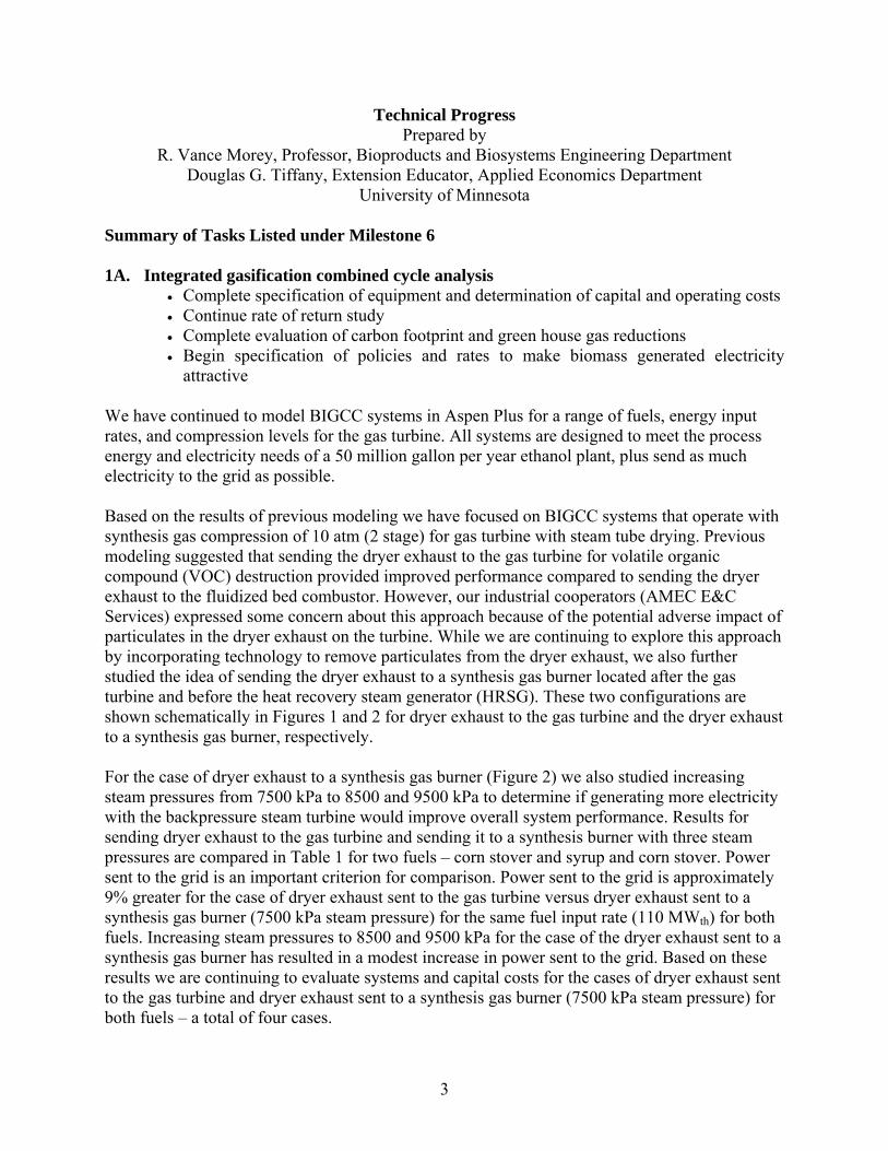
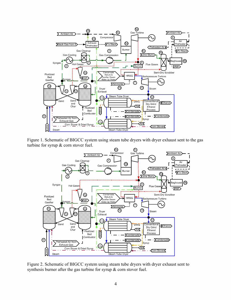
attractive We have continued to model BIGCC systems in Aspen Plus for a range of fuels, energy input rates, and compression levels for the gas turbine. All systems are designed to meet the process energy and electricity needs of a 50 million gallon per year ethanol plant, plus send as much electricity to the grid as possible. Based on the results of previous modeling we have focused on BIGCC systems that operate with synthesis gas compression of 10 atm (2 stage) for gas turbine with steam tube drying. Previous modeling suggested that sending the dryer exhaust to the gas turbine for volatile organic compound (VOC) destruction provided improved performance compared to sending the dryer exhaust to the fluidized bed combustor. However, our industrial cooperators (AMEC E&C Services) expressed some concern about this approach because of the potential adverse impact of particulates in the dryer exhaust on the turbine. While we are continuing to explore this approach by incorporating technology to remove particulates from the dryer exhaust, we also further studied the idea of sending the dryer exhaust to a synthesis gas burner located after the gas turbine and before the heat recovery steam generator (HRSG). These two configurations are shown schematically in Figures 1 and 2 for dryer exhaust to the gas turbine and the dryer exhaust to a synthesis gas burner, respectively. For the case of dryer exhaust to a synthesis gas burner (Figure 2) we also studied increasing steam pressures from 7500 kPa to 8500 and 9500 kPa to determine if generating more electricity with the backpressure steam turbine would improve overall system performance. Results for sending dryer exhaust to the gas turbine and sending it to a synthesis burner with three steam pressures are compared in Table 1 for two fuels – corn stover and syrup and corn stover. Power sent to the grid is an important criterion for comparison. Power sent to the grid is approximately 9% greater for the case of dryer exhaust sent to the gas turbine versus dryer exhaust sent to a synthesis gas burner (7500 kPa steam pressure) for the same fuel input rate (110 MWth) for both fuels. Increasing steam pressures to 8500 and 9500 kPa for the case of the dryer exhaust sent to a synthesis gas burner has resulted in a modest increase in power sent to the grid. Based on these results we are continuing to evaluate systems and capital costs for the cases of dryer exhaust sent to the gas turbine and dryer exhaust sent to a synthesis gas burner (7500 kPa steam pressure) for both fuels – a total of four cases.

4

Figure 1. Schematic of BIGCC system using steam tube dryers with dryer exhaust sent to the gas turbine for syrup & corn stover fuel.

Figure 2. Schematic of BIGCC system using steam tube dryers with dryer exhaust sent to synthesis burner after the gas turbine for syrup & corn stover fuel.

5

Table 1. System performances for 110 MW - 10 bar 2 stage (all fuel to gasifier)a,g .

aAll energy and power values are based on 110 MWth fuel Higher Heating Value(HHV). bThermal efficiency of converting fuel energy into other useful forms of energy (process heat and electricity), excludes BIGCC parasitic load. cPower use for parasitic BIGCC based on calculated power requirement for equipment (compressors, fans, pumps) and an electric motor efficiency of 95%. dTotal synthesis gas plus char equals 110 MWth. eIsentropic efficiency of gas turbine: 0.90, mechanical efficiency of gas turbine: 0.98. fIsentropic efficiency of air compressor: 0.85, mechanical efficiency of air compressor: 0.97 g Temperature of water leaving Economizer is 535 K, the temperature of steam leaving superheater is 755 K.

Stover Syrup and Stover Dryer Exhaust to

Gas Turbine

Syngas Burner after Turbine

Gas Turbine

Syngas Burner after Turbine

Pressure of Pump 7500kPa 7500kPa 8500kPa 9500 kPa 7500kPa 7500kPa 8500kPa 9500 kPa Generation Efficiency 30.6% 28.2% 28.4% 28.6% 30.6% 28.1% 28.3% 28.4% Thermal Efficiencyb 72.4% 70.5% 70.7% 71.0% 73.1% 71.2% 71.4% 71.6% Power Generation, MW Gas turbine totale 50.3 39.2 38.5 38.1 49.6 38.9 38.3 37.8 Shaft powerf 28.1 19.7 19.3 19.1 27.6 19.6 19.3 19.1 Gas turbine net power 22.2 19.5 19.2 19.0 22.0 19.3 19.0 18.7 Steam turbine 11.5 11.5 12.0 12.4 11.6 11.6 12.1 12.6 Total 33.7 31.0 31.2 31.4 33.6 30.9 31.1 31.3 Power Use, MW Ethanol process 4.7 4.7 4.7 4.7 4.7 4.7 4.7 4.7 Parasitic BIGCCc 4.5 3.9 3.9 3.9 4.4 3.7 3.7 3.7 To Grid 24.5 22.4 22.6 22.8 24.5 22.5 22.7 22.9 Total 33.7 31.0 31.2 31.4 33.6 30.9 31.1 31.3 Process Heat, MWth Ethanol process 27.9 27.9 27.9 27.9 27.9 27.9 27.9 27.9 Dryer 22.6 22.6 22.6 22.6 23.3 23.3 23.3 23.3 Total 50.5 50.5 50.5 50.5 51.2 51.2 51.2 51.2 Synthesis Gas Split, MWth Combustor 9.4 9.3 9.3 9.3 6.9 6.9 6.9 7.0 Turbine 75.7 61.8 60.8 60.1 76.7 62.6 61.7 60.8 After turbine 6.9 20.9 21.9 22.6 9.3 23.4 24.3 25.1 Totald 92.0 92.0 92.0 92.0 92.9 92.9 92.9 92.9 Combustor Input, MWth Chard 18.0 18.0 18.0 18.0 17.1 17.1 17.1 17.1 Syngas 6.9 9.3 9.3 9.3 6.9 6.9 6.9 7.0 Total 24.9 27.3 27.3 27.3 24.0 24.0 24.0 24.1 Combustor Output, MWth Gasifier heat duty 18.2 18.2 18.2 18.2 16.0 16.0 16.0 16.0 Combustion exhaust 6.7 9.1 9.1 9.3 8.0 8.0 8.0 8.1 Total 24.9 27.3 27.3 27.5 24.0 24.0 24.0 24.1 Condensate, Kg/hr 84,610 84,600 85,700 86,730 85,590 85,700 86,830 87,860

6

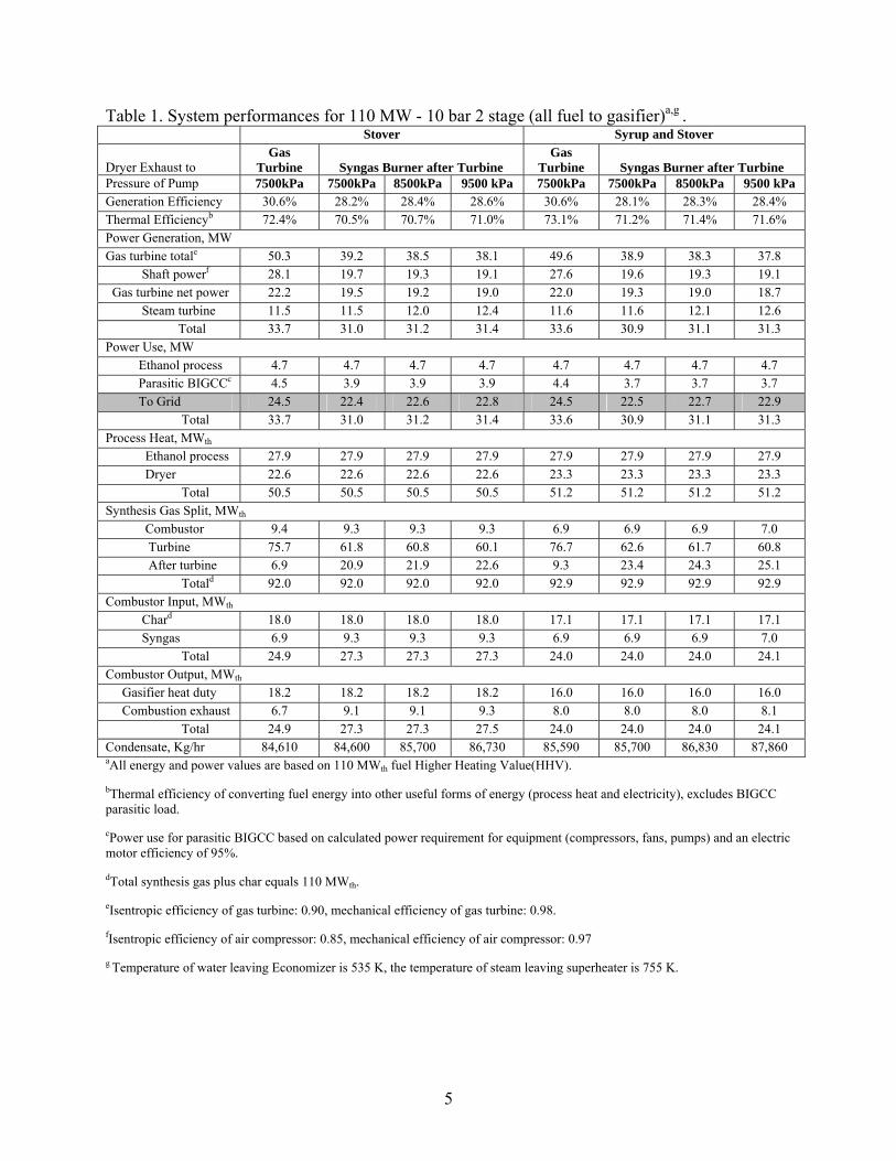
Economic Analysis of BIGCC Refinements in the Aspen Plus modeling resulted in the discovery of some better ideas in designing the process for the biomass integrated combined cycle (BIGCC) plant using biomass sources. However, these improvements in the design have had the effect of delayed cost estimation of key equipment needed by the BIGCC process to deliver high amounts of electricity and necessary process heat to run the model ethanol plants. To maintain progress on the project, modeling of economic performance was tested by first calculating some preliminary cost figures, with the full realization that more elegantly derived estimates of installed equipment costs would follow. This effort was made in the second half of May and the first half of June in 2010. Because the ethanol plant construction business was hit hard like many other construction activities in October of 2008 with the national crisis that occurred in nation’s financial markets, there have been far fewer observations of installed costs in what had been a very busy area of construction activity. Contact with Ron Fagen, CEO of Fagen, Incorporated, offered some insight into the installed costs that his firm was prepared to fulfill in June of 2010 for a 50 million gallon per year dry-grind ethanol plant. Instead of installed costs of $112,500,000 that had been typical in 2007, Mr. Fagen estimated installed costs of $75,000,000, representing a decline of 33%. By applying this same rate of decline to the equipment previously estimated for process heat, combined heat and power, and CHP + grid, it was possible to develop installed costs for the ethanol plant equipment and the additional equipment needed to handle biomass.

$‐

$20,000,000

$40,000,000

$60,000,000

$80,000,000

$100,000,000

$120,000,000

$140,000,000

$160,000,000

$180,000,000

$200,000,000

Estimated 2010 Installed Costs for Dry‐Grind 50MM GPY Conventional, Process Heat, CHP, CHP+Grid, and IGCC Using Natural Gas, Corn Stover, and Syrup + Stover

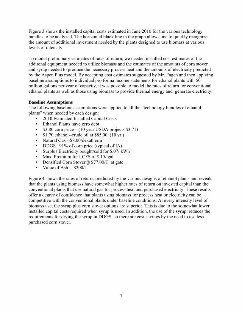
Figure 3. Estimated 2010 installed costs for 50 million gallon per year dry-grind ethanol plants including conventional natural gas and various biomass options.

7

Figure 3 shows the installed capital costs estimated in June 2010 for the various technology bundles to be analyzed. The horizontal black line in the graph allows one to quickly recognize the amount of additional investment needed by the plants designed to use biomass at various levels of intensity. To model preliminary estimates of rates of return, we needed installed cost estimates of the additonal equipment needed to utilize biomass and the estimates of the amounts of corn stover and syrup needed to produce the necessary process heat and the amounts of electricity predicted by the Aspen Plus model. By accepting cost estimates suggested by Mr. Fagen and then applying baseline assumptions to individual pro forma income statements for ethanol plants with 50 million gallons per year of capacity, it was possible to model the rates of return for conventional ethanol plants as well as those using biomass to provide thermal energy and generate electricity. Baseline Assumptions The following baseline assumptions were applied to all the “technology bundles of ethanol plants” when needed by each design:

• 2010 Estimated Installed Capital Costs • Ethanol Plants have zero debt • $3.80 corn price—(10 year USDA projects $3.71) • $1.70 ethanol--crude oil at $85.00, (10 yr.) • Natural Gas --$8.00/dekatherm • DDGS –91% of corn price (typical of IA) • Surplus Electricity bought/sold for $.07/ kWh • Max. Premium for LCFS of $.15/ gal. • Densified Corn Stover@ $77.00/T. at gate • Value of Ash is $200/T.

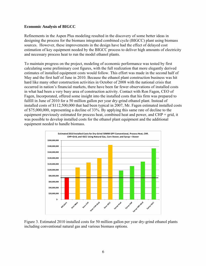
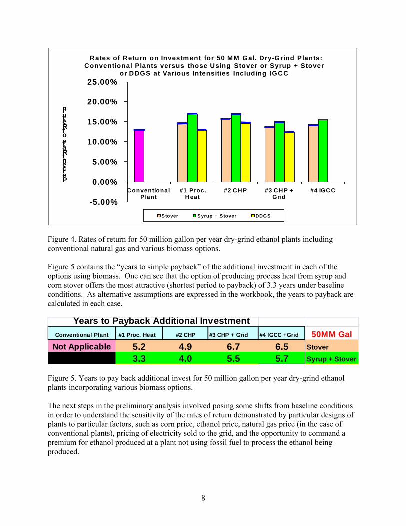
Figure 4 shows the rates of returns predicted by the various designs of ethanol plants and reveals that the plants using biomass have somewhat higher rates of return on invested capital than the conventional plants that use natural gas for process heat and purchased electricity. These results offer a degree of confidence that plants using biomass for process heat or electricity can be competitive with the conventional plants under baseline conditions. At every intensity level of biomass use, the syrup plus corn stover options are superior. This is due to the somewhat lower installed capital costs required when syrup is used. In addition, the use of the syrup, reduces the requirements for drying the syrup in DDGS, so there are cost savings by the need to use less purchased corn stover.

8

-5.00%

0.00%

5.00%

10.00%

15.00%

20.00%

25.00%

C onventional P lant

#1 Proc. H eat

#2 C H P #3 CH P + Grid

#4 IGC C

Percent Rate of Return

Rates of Return on Investment for 50 MM Gal. Dry-Grind Plants: Conventional Plants versus those Using Stover or Syrup + Stover

or DDGS at Various Intensities Including IGCC

S tover Syrup + S tover DDGS

Figure 4. Rates of return for 50 million gallon per year dry-grind ethanol plants including conventional natural gas and various biomass options. Figure 5 contains the “years to simple payback” of the additional investment in each of the options using biomass. One can see that the option of producing process heat from syrup and corn stover offers the most attractive (shortest period to payback) of 3.3 years under baseline conditions. As alternative assumptions are expressed in the workbook, the years to payback are calculated in each case. Years to Payback Additional Investment

Conventional Plant #1 Proc. Heat #2 CHP #3 CHP + Grid #4 IGCC +Grid 50MM GalNot Applicable 5.2 4.9 6.7 6.5 Stover

3.3 4.0 5.5 5.7 Syrup + Stover Figure 5. Years to pay back additional invest for 50 million gallon per year dry-grind ethanol plants incorporating various biomass options. The next steps in the preliminary analysis involved posing some shifts from baseline conditions in order to understand the sensitivity of the rates of return demonstrated by particular designs of plants to particular factors, such as corn price, ethanol price, natural gas price (in the case of conventional plants), pricing of electricity sold to the grid, and the opportunity to command a premium for ethanol produced at a plant not using fossil fuel to process the ethanol being produced.

9

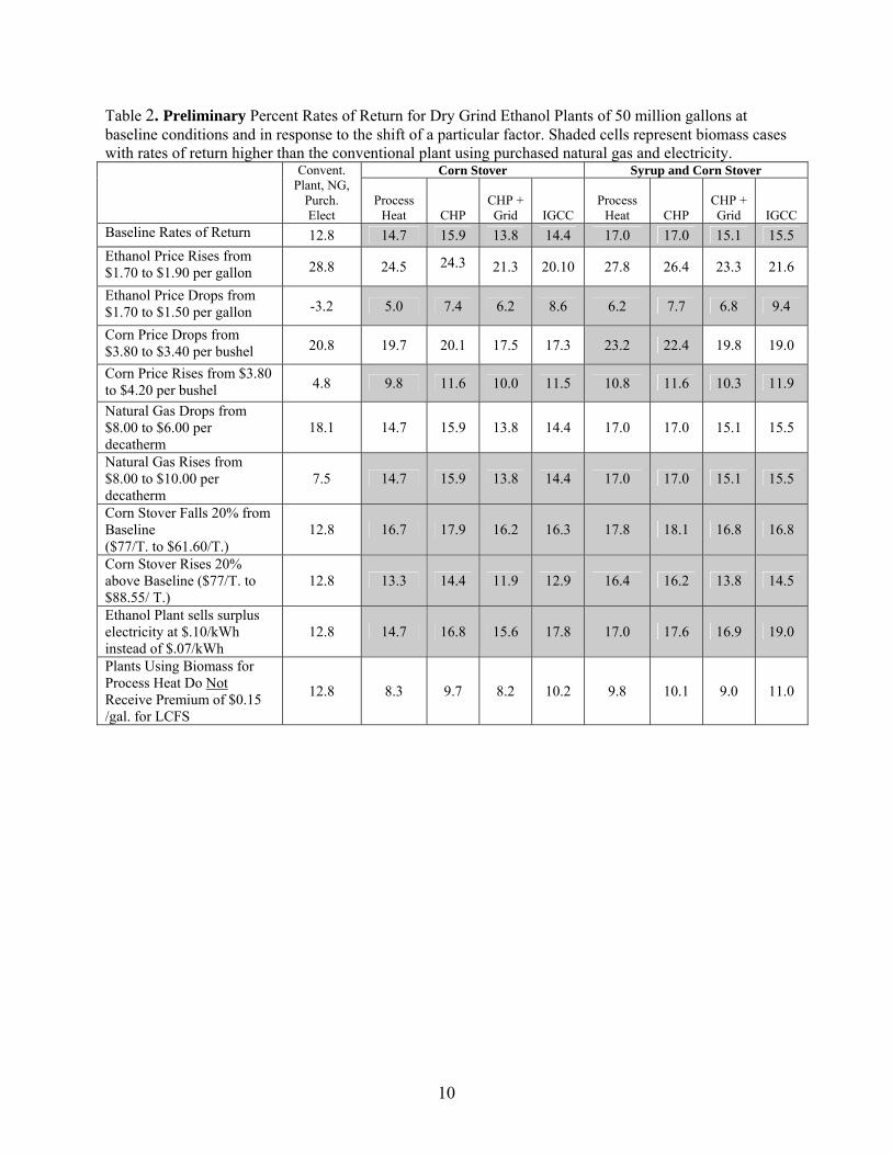
Discussion of Preliminary Rate of Return Results Table 2 shows rates of return on invested capital for the plants at baseline and for the key shifts that were modeled. At baseline conditions, the options that utilize biomass, whether stover alone or mixed with syrup, have higher rates of return than the typical dry-grind plants using natural gas and purchased electricity. When ethanol prices rise from $1.70 to $1.90 per gallon, the rates of return for all of the model plants rise; but the rate for the conventional plant increases the most because of lower capital costs. In contrast, when ethanol prices, drop from $1.70 to $1.50 the biomass-powered plants make more money due to the sale of electricity and the assumed premium of $0.15 per gallon of ethanol applied when the ethanol can be sold to states using a low carbon fuel standard. When corn prices drop, all plants make more money, but the syrup + stover plants producing process heat and CHP make the most. When corn prices rise, by $0.40 per bushel, the rate of return for the conventional plant drops dramatically to 4.75%, but the rates of return for the biomass-powered plants range from 9.8% to 11.94%. When natural gas prices drop from $8.00 to $6.00 per decatherm (one million BTUs), the rate of return for the conventional plant rises from 12.8% to 18.1 %, but the rates of return for the biomass-powered plants, stay at baseline levels. If natural gas price rises from $8.00 to $10.00 per decatherm, the biomass-powered plants stay at baseline levels, which are typically twice the rate of return of the conventional plant. Whether corn stover price rises by 20% or falls by 20%, the rates of return for the biomass-fired plants stay above the rate of return of the conventional plant. If ethanol plants are able to sell their surplus electricity at $0.10 per kWh instead of the baseline level of $0.07, the rates of return are enhanced for all options that produce electricity. The last factor studied in sensitivity analysis is the consideration of whether or not the plants receive a premium on the ethanol they sell due to measures such as the low carbon fuel standards being enacted by several states. If ethanol plants using corn stover or syrup are excluded by state regulations, the rates of return for the plants using biomass fall substantially from the baseline levels. As states make their determinations of what ethanol can be sold within their borders, plants considering technologies that use biomass should request a letter ruling on this question.

10

Table 2. Preliminary Percent Rates of Return for Dry Grind Ethanol Plants of 50 million gallons at baseline conditions and in response to the shift of a particular factor. Shaded cells represent biomass cases with rates of return higher than the conventional plant using purchased natural gas and electricity.

Corn Stover Syrup and Corn Stover Convent. Plant, NG,

Purch. Elect

Process Heat CHP

CHP + Grid IGCC

Process Heat CHP

CHP + Grid IGCC

Baseline Rates of Return 12.8 14.7 15.9 13.8 14.4 17.0 17.0 15.1 15.5 Ethanol Price Rises from $1.70 to $1.90 per gallon 28.8 24.5 24.3 21.3 20.10 27.8 26.4 23.3 21.6

Ethanol Price Drops from $1.70 to $1.50 per gallon -3.2 5.0 7.4 6.2 8.6 6.2 7.7 6.8 9.4

Corn Price Drops from $3.80 to $3.40 per bushel 20.8 19.7 20.1 17.5 17.3 23.2 22.4 19.8 19.0

Corn Price Rises from $3.80 to $4.20 per bushel 4.8 9.8 11.6 10.0 11.5 10.8 11.6 10.3 11.9

Natural Gas Drops from $8.00 to $6.00 per decatherm

18.1 14.7 15.9 13.8 14.4 17.0 17.0 15.1 15.5

Natural Gas Rises from $8.00 to $10.00 per decatherm

7.5 14.7 15.9 13.8 14.4 17.0 17.0 15.1 15.5

Corn Stover Falls 20% from Baseline ($77/T. to $61.60/T.)

12.8 16.7 17.9 16.2 16.3 17.8 18.1 16.8 16.8

Corn Stover Rises 20% above Baseline ($77/T. to $88.55/ T.)

12.8 13.3 14.4 11.9 12.9 16.4 16.2 13.8 14.5

Ethanol Plant sells surplus electricity at $.10/kWh instead of $.07/kWh

12.8 14.7 16.8 15.6 17.8 17.0 17.6 16.9 19.0

Plants Using Biomass for Process Heat Do Not Receive Premium of $0.15 /gal. for LCFS

12.8 8.3 9.7 8.2 10.2 9.8 10.1 9.0 11.0

11

1C. Integration of superheated steam dryer technology • Continue evaluation of rate of return

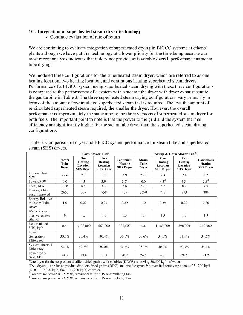
We are continuing to evaluate integration of superheated drying in BIGCC systems at ethanol plants although we have put this technology at a lower priority for the time being because our most recent analysis indicates that it does not provide as favorable overall performance as steam tube drying. We modeled three configurations for the superheated steam dryer, which are referred to as one heating location, two heating location, and continuous heating superheated steam dryers. Performance of a BIGCC system using superheated steam drying with these three configurations is compared to the performance of a system with a steam tube dryer with dryer exhaust sent to the gas turbine in Table 3. The three superheated steam drying configurations vary primarily in terms of the amount of re-circulated superheated steam that is required. The less the amount of re-circulated superheated steam required, the smaller the dryer. However, the overall performance is approximately the same among the three versions of superheated steam dryer for both fuels. The important point to note is that the power to the grid and the system thermal efficiency are significantly higher for the steam tube dryer than the superheated steam drying configurations. Table 3. Comparison of dryer and BIGCC system performance for steam tube and superheated steam (SHS) dryers.

Corn Stover Fuela Syrup & Corn Stover Fuelb Steam Tube Dryer

One Heating Location

SHS Dryer

Two Heating Location

SHS Dryer

Continuous Heating

SHS Dryer

Steam Tube Dryer

One Heating Location

SHS Dryer

Two Heating Location

SHS Dryer

Continuous Heating

SHS Dryer

Process Heat, MW 22.6 2.2 2.5 2.9 23.3 2.3 2.4 3.2

Power, MW 0.0 4.3c 3.9c 3.7c 0.0 4.5d 4.3d 3.8d Total, MW 22.6 6.5 6.4 6.6 23.3 6.7 6.7 7.0 Energy, kJ/kg water removed 2660 765 759 779 2690 778 773 804

Energy Relative to Steam Tube Dryer

1.0 0.29 0.29 0.29 1.0 0.29 0.29 0.30

Water Recov., liter water/liter ethanol

0 1.3 1.3 1.3 0 1.3 1.3 1.3

Re-circulated SHS, kg/h n.a. 1,138,000 563,000 306,500 n.a. 1,189,000 598,000 312,000

Power Generation Efficiency

30.6% 30.4% 30.4% 30.5% 30.6% 31.0% 31.1% 31.6%

System Thermal Efficiency 72.4% 49.2% 50.0% 50.6% 73.1% 50.0% 50.3% 54.1%

Power to the Grid, MW 24.5 19.4 19.9 20.2 24.5 20.1 20.6 21.2 aOne dryer for the co-product distillers dried grains with solubles (DDGS) removing 30,650 kg/h of water. bTwo dryers – one for co-product distillers dried grains (DDG) and one for syrup & stover fuel removing a total of 31,200 kg/h (DDG – 17,300 kg/h, fuel – 13,900 kg/h) of water. cCompressor power is 3.5 MW, remainder is for SHS re-circulating fan. dCompressor power is 3.6 MW, remainder is for SHS re-circulating fan.

12

The ethanol process including fuel and co-product drying provides a place to exhaust waste heat, which is required for electricity generation. If less energy is required for drying, then there is less demand for waste heat; therefore, less electricity can be generated in order for the system to be in balance. If electricity generation were not a goal of the application, requiring a place to dump waste heat, then superheated steam drying would have advantages both in terms of reduced energy use and water demand. The primary attraction is the potential to reduce the water requirement for ethanol production by about 1.3 gallons of water/gallon of ethanol. This is not possible with steam tube drying because the water leaves as vapor in the drying air and is not easily recaptured. Current dry-grind ethanol production technology requires on the order of 2.7 to 3.7 gallons of water/gallon of ethanol at the plant. Thus, implementing superheated steam dryer technology could reduce the requirement to the range of 1.4 to 2.4 gallons of water/gallon of ethanol.

13

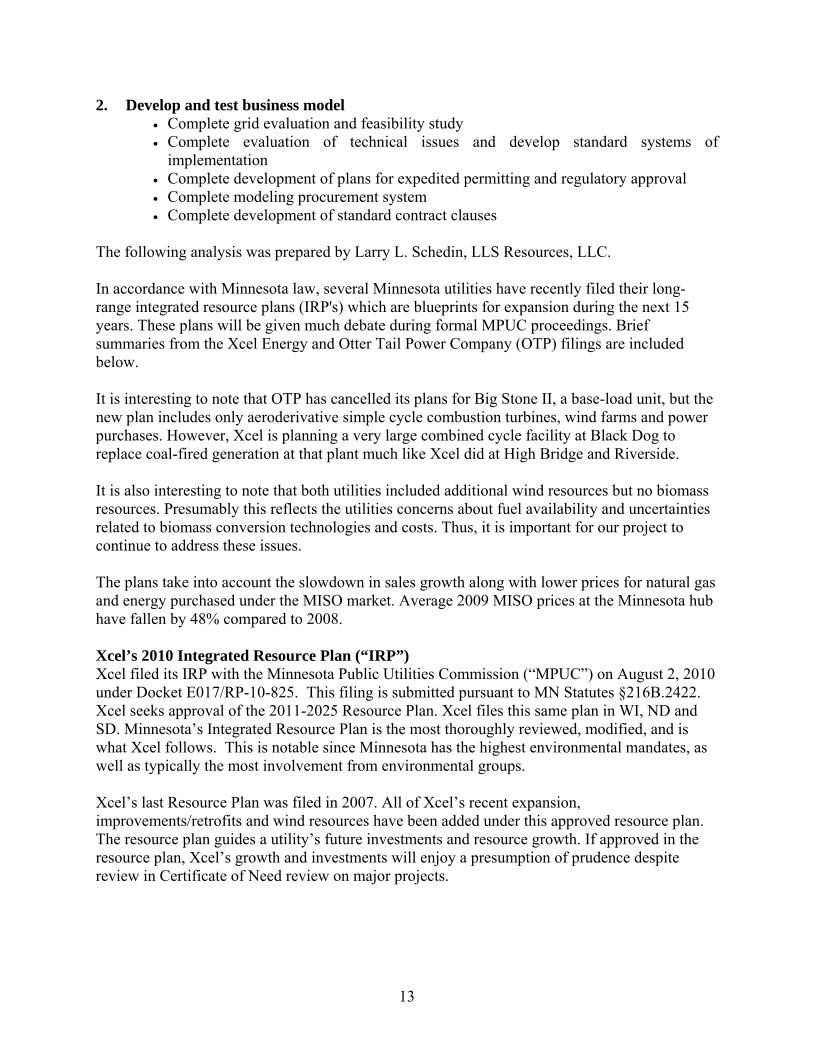
2. Develop and test business model • Complete grid evaluation and feasibility study • Complete evaluation of technical issues and develop standard systems of

implementation • Complete development of plans for expedited permitting and regulatory approval • Complete modeling procurement system • Complete development of standard contract clauses

The following analysis was prepared by Larry L. Schedin, LLS Resources, LLC. In accordance with Minnesota law, several Minnesota utilities have recently filed their long-range integrated resource plans (IRP's) which are blueprints for expansion during the next 15 years. These plans will be given much debate during formal MPUC proceedings. Brief summaries from the Xcel Energy and Otter Tail Power Company (OTP) filings are included below. It is interesting to note that OTP has cancelled its plans for Big Stone II, a base-load unit, but the new plan includes only aeroderivative simple cycle combustion turbines, wind farms and power purchases. However, Xcel is planning a very large combined cycle facility at Black Dog to replace coal-fired generation at that plant much like Xcel did at High Bridge and Riverside. It is also interesting to note that both utilities included additional wind resources but no biomass resources. Presumably this reflects the utilities concerns about fuel availability and uncertainties related to biomass conversion technologies and costs. Thus, it is important for our project to continue to address these issues. The plans take into account the slowdown in sales growth along with lower prices for natural gas and energy purchased under the MISO market. Average 2009 MISO prices at the Minnesota hub have fallen by 48% compared to 2008. Xcel’s 2010 Integrated Resource Plan (“IRP”) Xcel filed its IRP with the Minnesota Public Utilities Commission (“MPUC”) on August 2, 2010 under Docket E017/RP-10-825. This filing is submitted pursuant to MN Statutes §216B.2422. Xcel seeks approval of the 2011-2025 Resource Plan. Xcel files this same plan in WI, ND and SD. Minnesota’s Integrated Resource Plan is the most thoroughly reviewed, modified, and is what Xcel follows. This is notable since Minnesota has the highest environmental mandates, as well as typically the most involvement from environmental groups. Xcel’s last Resource Plan was filed in 2007. All of Xcel’s recent expansion, improvements/retrofits and wind resources have been added under this approved resource plan. The resource plan guides a utility’s future investments and resource growth. If approved in the resource plan, Xcel’s growth and investments will enjoy a presumption of prudence despite review in Certificate of Need review on major projects.

14

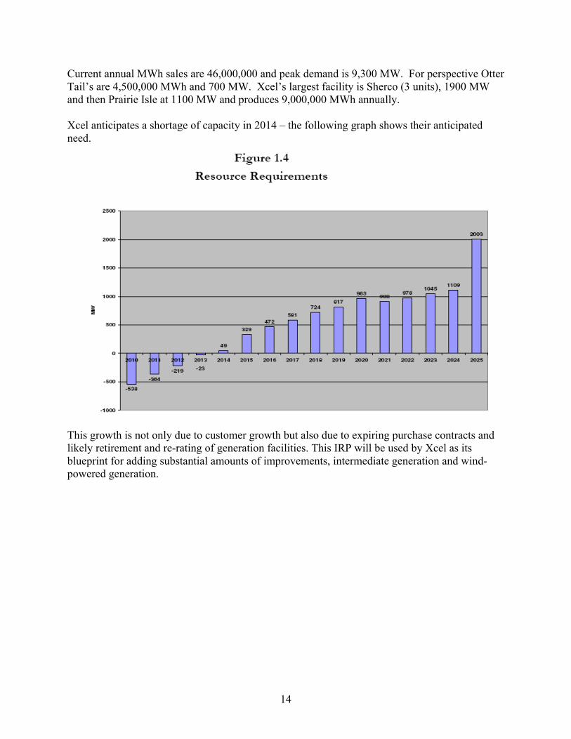
Current annual MWh sales are 46,000,000 and peak demand is 9,300 MW. For perspective Otter Tail’s are 4,500,000 MWh and 700 MW. Xcel’s largest facility is Sherco (3 units), 1900 MW and then Prairie Isle at 1100 MW and produces 9,000,000 MWh annually.

Xcel anticipates a shortage of capacity in 2014 – the following graph shows their anticipated need.

This growth is not only due to customer growth but also due to expiring purchase contracts and likely retirement and re-rating of generation facilities. This IRP will be used by Xcel as its blueprint for adding substantial amounts of improvements, intermediate generation and wind-powered generation.

15

The following table shows how they propose to meet that need

The following table shows their anticipated cost increases under this plan.

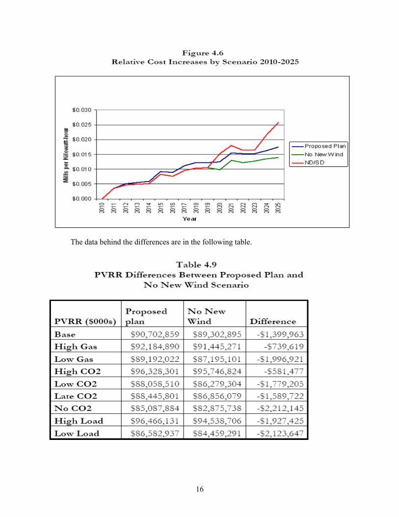
Their proposed plan is not “least cost”, it is the plan which allows them to satisfy the RES requirements. They have chosen not to test the “off ramp” provision in statute. The following chart shows the relationship of the preferred plan and least cost plan.

16

The data behind the differences are in the following table.

17

Xcel is not selecting its least cost plan due to forcing wind selection. This is demonstrated by the above chart and discussions with Xcel that indicate, even assuming all externalities and DSM requirements, departure from wind RES would result in savings. This presents a question of timing on when to test the “off ramp” built into statute.

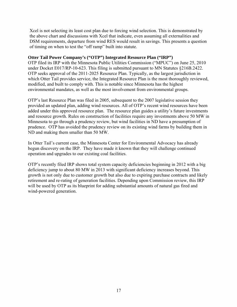
Otter Tail Power Company’s (“OTP”) Integrated Resource Plan (“IRP”) OTP filed its IRP with the Minnesota Public Utilities Commission (“MPUC”) on June 25, 2010 under Docket E017/RP-10-623. This filing is submitted pursuant to MN Statutes §216B.2422. OTP seeks approval of the 2011-2025 Resource Plan. Typically, as the largest jurisdiction in which Otter Tail provides service, the Integrated Resource Plan is the most thoroughly reviewed, modified, and built to comply with. This is notable since Minnesota has the highest environmental mandates, as well as the most involvement from environmental groups.

OTP’s last Resource Plan was filed in 2005, subsequent to the 2007 legislative session they provided an updated plan, adding wind resources. All of OTP’s recent wind resources have been added under this approved resource plan. The resource plan guides a utility’s future investments and resource growth. Rules on construction of facilities require any investments above 50 MW in Minnesota to go through a prudency review, but wind facilities in ND have a presumption of prudence. OTP has avoided the prudency review on its existing wind farms by building them in ND and making them smaller than 50 MW.

In Otter Tail’s current case, the Minnesota Center for Environmental Advocacy has already begun discovery on the IRP. They have made it known that they will challenge continued operation and upgrades to our existing coal facilities.

OTP’s recently filed IRP shows total system capacity deficiencies beginning in 2012 with a big deficiency jump to about 80 MW in 2013 with significant deficiency increases beyond. This growth is not only due to customer growth but also due to expiring purchase contracts and likely retirement and re-rating of generation facilities. Depending upon Commission review, this IRP will be used by OTP as its blueprint for adding substantial amounts of natural gas fired and wind-powered generation.

18

3. Analysis of a biomass procurement system • Continue specification of equipment and determination of capital and operating costs • Continue rate of return on investment study

One of the key elements of the corn stover supply logistics system is a process to coarsely grind the stover and then roll compact it to achieve a bulk density of at least 15 lbs/ft3, which will allow trucks to load out at a 25 ton limit. We have conducted laboratory compression tests on biomass and pilot scale tests of a roll compaction system. One of our goals is to be able to predict performance of roll compaction systems. The following results summarize our attempts to develop and validate model to predict roll compaction performance of biomass. The objective of this task is to validate the roll press design equations given by Johanson (1965) and Blake et al. (1963) using the data collected from the pilot-scale roll press compaction study conducted at Bepex International LLC, and the data collected from the laboratory compaction study. The validated roll press design equations will be used for deriving design specifications for a production scale (25 ton/h) roll press compactor. Roll Press Compactor Design Equations Johanson (1965) Model Johanson (1965) established relationships for roll force (Rf) and roll torque (Rt) as functions of roll pressure (P), roll diameter (D), roll width (W), roll gap (Rg), and compressibility factor (K). The roll gap (Rg) is the sum of two times the depth of pockets on one of the rolls (d/2) plus the pre-set roll gap (S) [i.e., Rg = d + S]. It is noted that the pre-set roll gap (S) changes during the pilot-scale roll press experiments due to the floating of one of the rolls. The equation for roll force is (Johanson, 1965):

Rf = P W D Ff / 2 (1) Where, Rf = roll separating force (MN); P = applied pressure that may produce the required density of compact (obtained from the uniaxial compression test) (MPa); W = roll width (m); D = roll diameter (m); and Ff = force factor, estimated as a function of D, d, S, and K (Johanson, 1965).

(2)

The equation for roll torque is (Johanson, 1965):

Rt = P W D2 Tf / 8 (3) Where, Tf = torque factor, estimated as a function of D, d, S, and K (Johanson, 1965).

19

(4)

The force factor and torque factor integrals are evaluated numerically using trapezoidal rule (Cheney and Kincaid, 1985). In this study, these integrals are evaluated for a maximum angle of θ where P is about zero (i.e., θ =α = 60°). Johanson (1965) derived the following relationship between the pressure and density for compaction of powdered materials during uniaxial compression in laboratory compaction apparatus.

(ρ/ρo) = (P/Po)(1/K) (5) Where, ρ is compact density (out-of-the die density after curing one week at room temperature) at pressure P, and K is the compressibility factor of powdered material. Using the above relationship, the roll pressure required to produce a compact with a prescribed compact density is estimated. Blake et al. (1963) Model Blake et al. (1963) modeled the force between the rolls (Rf) as a function of the diameter (D) of the rolls, the width of the rolls (W), the angle θ subtended at the center of the roll by a particular position of an element of powdered material and the horizontal, and the actual pressure P on the element of material at angle θ. The force between the rolls (Rf) is (Blake et al., 1963):

(6)

From the roll force, the torque on each roll (Rt) can be calculated as:

(7) Where, P is the actual pressure on an element of material at an angle θ measured upward from the center of the rolls. The angle θ is zero at the horizontal line connecting the centers of the rolls. The roll force and roll torque integrals can be evaluated if P is known as a function of θ. The integrals are evaluated numerically using trapezoidal rule (Cheney and Kincaid, 1985). In this study, the integrals are evaluated for a maximum angle of θ where P is about zero. To get the relation between P and θ, it is first necessary to assume a maximum pressure (Pmax). For this assumed maximum pressure, laboratory compaction test is conducted to get a compression curve between P and ΔL/L. Where, L is the thickness of the compact (in-die) at the maximum pressure, and ΔL is the difference between the compact thickness (in-die) at the maximum pressure and the compact thickness (in-die) at any other pressure. For the assumed maximum compression pressure, a polynomial relationship between P and ΔL/L is established.

20

If L is the minimum roll gap (i.e., the thickness of compact at the minimum roll gap = Rg = d + S), then, from the geometry of the rolls, ΔL/L = D/L [1 – cos θ]. The expressions for ΔL/L for the roll press and the lab compaction can be equated, and they provide the relation between P and θ. While numerical integration of the roll force and torque equations, a value for θ is chosen and ΔL/L for the roll press is calculated; using this ΔL/L value, the corresponding pressure is obtained from the polynomial relationship between P and ΔL/L for the lab compaction data. With the integrals evaluated, the roll force and torque corresponding to the assumed maximum pressure is readily calculated. In this manner, a linear relationship between the roll force or torque and the maximum compaction pressure can be derived for a given roll press compactor specifications (D, W, and L). Throughput, Power, and Specific Energy Consumption The theoretical relationships for calculating throughput of roll press compactor, roll motor power, and specific energy consumption for operation of the rolls are given below.

Throughput of roll press compactor (Cc) = 60 ρg π D W Rg Rs / 1000 (8) Where, Cc = throughput of roll compactor (t/h), ρg = density of roll press compacts at the minimum roll gap before exiting the rolls (kg m-3), D = roll diameter (m), W = roll width (m), Rg = roll gap (m) (two half-pocket depths plus gap between rolls), and Rs = roll speed (rpm). ρg is calculated based on the mass of biomass compacted per unit time (i.e., throughput) and the theoretical volume of the roll press compactor that caused this throughput. The volume is calculated as a function of D, W, Rg, and Rs.

Roll motor power required for operating two rolls (Rp) = 2 Rt ω (9) Where, Rp = roll power (MW), Rt = roll torque (MN-m) estimated based on Johanson (1965) model or Blake et al. (1963) model, ω = (2 π Rs / 60), ω = angular velocity of rolls (s-1), and Rs = roll speed (rpm). Please note that 1 MW = 1340.483 hp.

Specific energy consumption (MJ/t) for operating two rolls (Rse) = 3600 Rp / Cc (10) Where, Rp = roll power (MW), and Cc = throughput of roll compactor (t/h) Experimental Data From the pilot-scale roll press compaction experiments conducted at Bepex International LLC, we have collected data on roll diameter (D = 0.521 m), roll width (W = 0.127 m), roll gap (Rg = L = 0.012 m or 0.022 m), roll speed (Rs), throughput (Cc), and specific energy consumption (Rse) for roll-press compaction of corn stover and native perennial grasses. According to the roll pocket dimension (d = 2 x 5.1 mm) and set roll gap (2.03 mm), the minimum roll gap (Rg or L) is 0.012 m. However, the minimum roll gap increased during the roll press operation due to the floating of one of the rolls. Thus, assuming a maximum floating roll displacement of 10.0 mm, modeling results are calculated for another minimum roll gap (Rg or L) of 0.022 m.

21

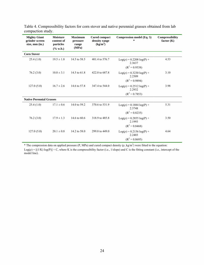
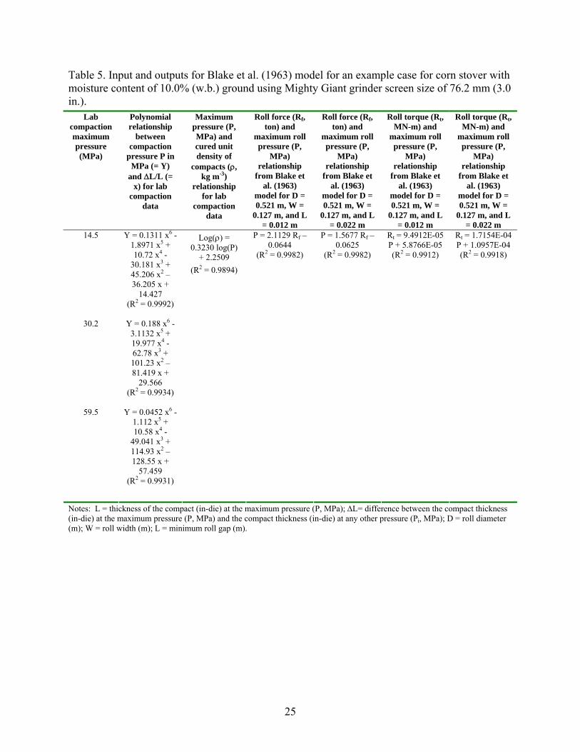
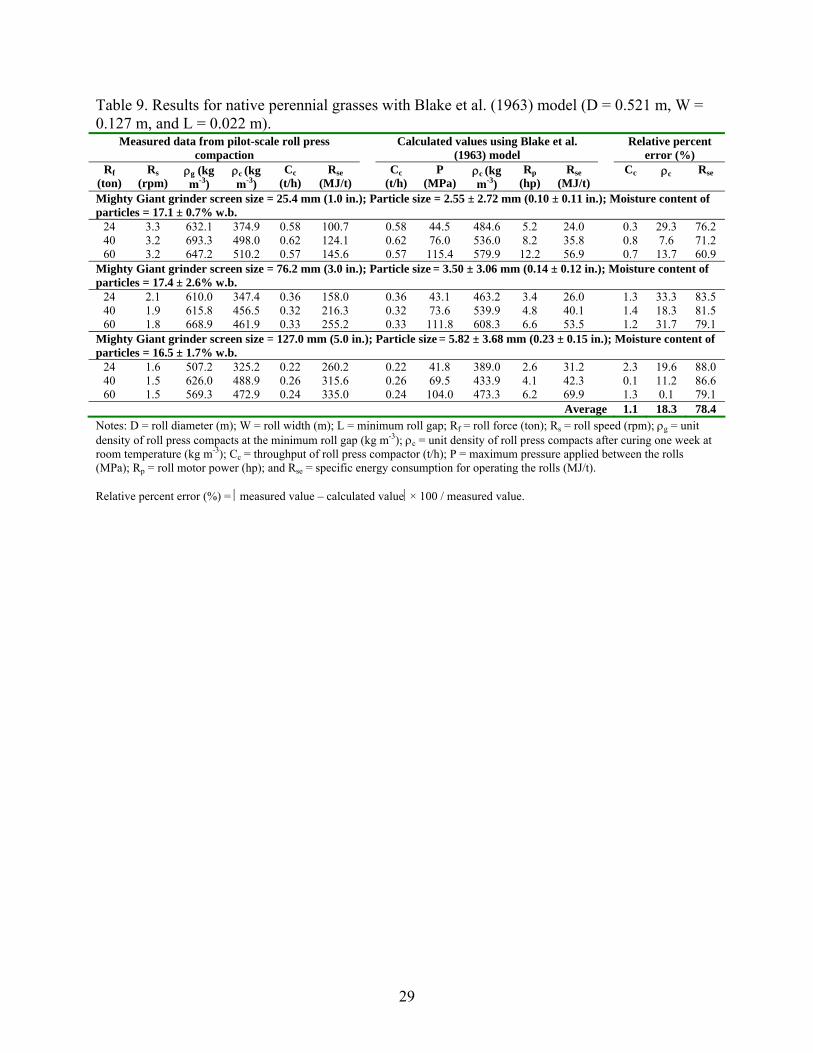
The lab compaction study is conducted for three maximum compression pressures of about 15, 30, and 60 MPa for corn stover and perennial grass particles obtained from three Mighty Giant grinder screen sizes (25.4, 76.2, and 127.0 mm). From the lab compaction data, compressibility factors (K) for corn stover and perennial grasses are estimated (Table 4). The compressibility factors are used in the Johanson (1965) model. Also, polynomial relationships between maximum compaction pressure P and ΔL/L for lab compaction data are obtained to use in Blake et al. (1963) model. An example calculation involved for Blake et al. (1963) model is given in Table 5. The roll press design equations are validated for pilot-scale roll press compaction data collected for two biomass materials (corn stover and native perennial grasses) ground using three Mighty Giant grinder screen sizes (25.4, 76.2, and 127.0 mm), three roll forces (24, 40, and 60 ton), and two minimum roll gap sizes (Rg = L = 0.012 m or 0.022 m). Validation of Johanson (1965) Model To validate the roll force calculated using Johanson (1965) model, first it is assumed that the maximum pressure required to produce compacts with a given unit density (measured after curing one-week at room temperature) is the same for roll press compaction and lab compaction. Using the lab compaction data, a relationship between maximum pressure and unit density of compacts (cured) is established (Eq. 5). From this relationship between pressure and cured density, for each pilot-scale roll press experiment, the maximum roll pressure (P) that may have been applied to the rolls is calculated for the measured (cured) unit density of roll press compacts. Then, the roll force is calculated using Johanson (1965) model (Eq. 1) by inputting the maximum roll pressure (P) to the Eq. 1. Finally, this calculated roll force and the actual roll force applied to the rolls during the pilot-scale roll press experiments are compared. Similarly, for a given maximum roll pressure (P), the roll torque is calculated using Eq. 3. The calculated roll torque is used to estimate the roll power (Eq. 9) and specific energy consumption for the rolls (Eq. 10). Then, the calculated and measured specific energy consumption values are compared. The throughput of the roll press compactor is calculated using Eq. 8 and compared with the measured data. Validation of Blake et al. (1963) Model To validate the Blake et al. (1963) model, first it is assumed that the maximum pressure required to produce compacts with a given unit density (measured after curing one-week at room temperature) is the same for roll press compaction and lab compaction. Using the lab compaction data, a relationship between maximum pressure and unit density of compacts (cured) is established (Eq. 5). Then, using the linear relationship established between the roll force [calculated using Blake et al. (1963) model] and the maximum pressure, the maximum pressure experienced by the rolls is calculated for an applied roll force. Applied roll force is used to calculate the roll pressure due to the fact that the material experiences the applied roll force during the roll press operation as indicated by floating of one of the rolls. From the relationship

22

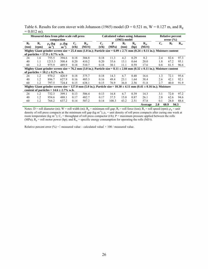
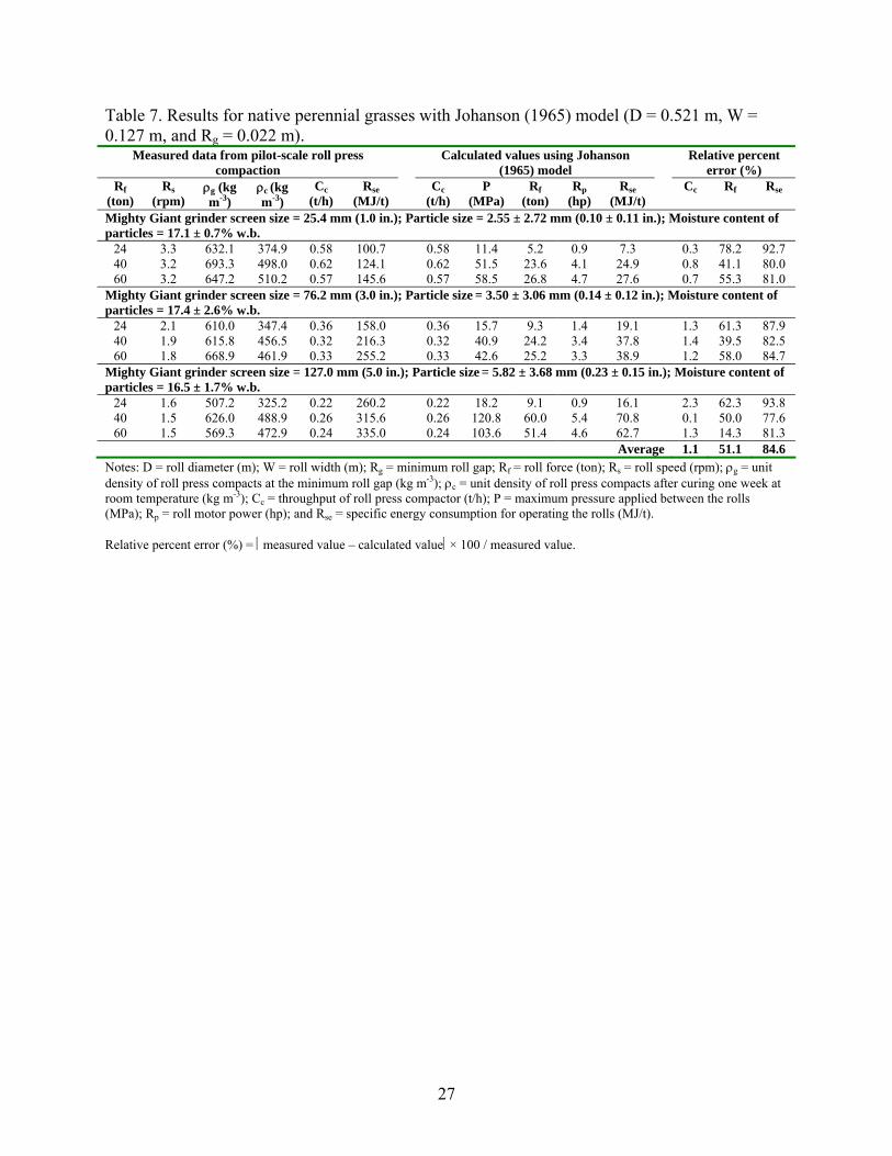
between pressure and cured density (Eq. 5), for each pilot-scale roll press experiment, the cured density of compact is calculated by inputting the calculated maximum roll pressure (due to the applied force). Finally, the calculated and measured (cured) unit densities of roll press compacts are compared. The roll torque is calculated using the linear relationship established between the roll torque [calculated using Blake et al. (1963) model] and the maximum roll pressure. The calculated roll torque is used to estimate the roll power (Eq. 9) and specific energy consumption for the rolls (Eq. 10). Then, the calculated and measured specific energy consumption values are compared. The throughput of the roll press compactor is calculated using Eq. 8 and compared with the measured data. Results and Discussion Tables 6 and 7 provide example results for Johanson (1965) model validation for corn stover and native perennial grasses, respectively. Tables 8 and 9 provide example results for Blake et al. (1963) model validation for corn stover and native perennial grasses, respectively. The throughput of the roll press is calculated with 1.1 to 2.0% of mean relative percent error by using the at-the-minimum-gap unit density of roll press compacts in the throughput model (Eq. 8). For validation of both models, increasing the minimum roll gap (Rg or L) from 0.012 m to 0.022 m decreased the mean relative percent error for the calculation of roll force, cured unit density of compacts, and specific energy consumption for rolls. This indicates that the minimum roll gap during operation of the roll press may have been larger than the pre-set roll gap (i.e., 0.012 m). The measured thickness of compacts (after curing) ranged from 20.0 to 27.7 mm for corn stover and from 25.1 to 37.0 mm for perennial grasses. Thus, the measured thicknesses of compacts also suggest that the roll gap changed during the operation of roll press. The change in roll gap may be affected by the screw feeder operation. Therefore, the minimum roll gap needs to be measured accurately for better validation of roll press design equations. The average compressibility factor (K) is 3.87 and 4.48 for corn stover and native perennial grasses, respectively. The lower K value for corn stover indicates that corn stover is easier to compress than perennial grasses (Johanson, 1965). Johanson (1965) model calculates the roll force with a mean relative percent error of 46.5 to 60.9%. One reason for predicting the roll force with a higher mean relative percent error is that Johanson (1965) model considers only the densification effect on the roll force and neglects the effect of elastic spring-back of compacts on the roll force. Peter et al. (2010) reported that the roll force due to elastic spring-back of compacts in the roll press can be as much as 30% of the total roll force. Yusof et al. (2005) found that Johanson (1965) model predicted the roll force and roll torque with an accuracy of 20% for maize powder with compressibility factor of 9.0. Dec et al. (2003) concluded that Johanson (1965) model predicts the roll force and roll torque with larger errors (as much as 50%) for materials with low compressibility factors.

23

Blake et al. (1963) model predicts the (cured) unit density of roll press compacts with a mean relative percent error of 18.3 to 30.0%. Although it appears Blake et al. (1963) model is more accurate than Johanson (1965) model, it should be noted that both models ignore the effect of shear forces that would occur during the roll press compaction. Also, modeling results may be affected by the possible measurement errors that may have happened during roll press compaction and lab compaction studies. Johanson (1965) model calculates the maximum roll power requirement of 5.4 hp. Blake et al. (1963) model predicts the maximum roll power requirement of 12.2 hp. The mean relative percent error in prediction of specific energy consumption for rolls is 84.6 to 94.3% for Johanson (1965) model and 78.4 to 91.2% for Blake et al. (1963) model. It is noted that these two theoretical models do not include inefficiency of the roll press system such as efficiency of the motor and speed reduction. The pilot-scale roll press was operated with a 50 hp motor and was designed to operate as high as 20 rpm whereas the maximum roll speed involved in our study was 3.3 rpm. Also, the measured specific energy consumption data showed that about 52 to 87% of the measured specific energy was required to operate the empty (i.e., no-load) roll press. Thus, including a motor efficiency, the roll press design models may result in reasonable estimates for roll motor power requirement and specific energy consumption for rolls. Conclusions and Future Work • Johanson (1965) model predicts the roll force with a mean relative percent error of 47 to

61%. • Blake et al. (1963) model calculates the unit density of compacts (measured after curing)

with a mean relative percent error of 18 to 30%. • Both Johanson (1965) and Blake et al. (1963) models may be used to obtain reasonable

estimates on the roll power requirement and specific energy consumption for the operation of rolls.

• Future work is planned to validate the Johanson (1965) and Blake et al. (1963) models using the measured data from a demonstration scale roll press compaction study.

References Blake, J.H., R.G. Minet, and W.P. Steen. 1963. Pressure developed in a roll-type briquet press.

Proceedings of the 8th IBA Biennial Briquetting Conference. pp. 38-48. Cheney, W., and D. Kincaid. 1985. Numerical Mathematics and Computing. Monterey, Cal.:

Brooks/Cole Publishing. Dec, R.T., A. Zavaliangos, and J.C. Cunningham. 2003. Comparison of various methods for

analysis of powder compaction in roller press. Powder Technology 130(1-3): 265-271. Johanson, J.R. 1965. A rolling theory for granular solids. Transactions of the ASME Journal of

Applied Mechanics 32(4): 842-848. Peter, S., R.F. Lammens, and K.J. Steffens. 2010. Roller compaction/dry granulation: Use of the

thin layer model for predicting densities and forces during roller compaction. Powder Technology 199(2): 165-175.

Yusof, Y.A., A.C. Smith, and B.J. Briscoe. 2005. Roll compaction of maize powder. Chemical Engineering Science 60(14): 3919-3931.

24

Table 4. Compressibility factors for corn stover and native perennial grasses obtained from lab compaction study.

Mighty Giant grinder screen size, mm (in.)

Moisture content of particles (% w.b.)

Maximum pressure

range (MPa)

Cured compact density range

(kg/m3)

Compression model (Eq. 5) *

Compressibility factor (K)

Corn Stover

25.4 (1.0) 19.5 ± 1.8 14.5 to 58.5 401.4 to 576.7 Log(ρ) = 0.2208 log(P) + 2.3637

(R2 = 0.9538)

4.53

76.2 (3.0) 10.0 ± 3.1 14.5 to 61.8 422.0 to 687.8 Log(ρ) = 0.3230 log(P) + 2.2509

(R2 = 0.9894)

3.10

127.0 (5.0) 16.7 ± 2.6 14.6 to 57.8 347.4 to 544.0 Log(ρ) = 0.2512 log(P) + 2.2932

(R2 = 0.7853)

3.98

Native Perennial Grasses

25.4 (1.0) 17.1 ± 0.6 14.0 to 59.2 370.6 to 531.9 Log(ρ) = 0.1884 log(P) + 2.3748

(R2 = 0.8235)

5.31

76.2 (3.0) 17.9 ± 1.3 14.6 to 60.6 318.9 to 485.8 Log(ρ) = 0.2855 log(P) + 2.1993

(R2 = 0.8468)

3.50

127.0 (5.0) 20.1 ± 0.8 14.2 to 58.0 299.8 to 449.0 Log(ρ) = 0.2156 log(P) + 2.2403

(R2 = 0.8695)

4.64

* The compression data on applied pressure (P, MPa) and cured compact density (ρ, kg/m3) were fitted to the equation: Log(ρ) = [(1/K) log(P)] + C, where K is the compressibility factor (i.e., 1/slope) and C is the fitting constant (i.e., intercept of the model line).

25

Table 5. Input and outputs for Blake et al. (1963) model for an example case for corn stover with moisture content of 10.0% (w.b.) ground using Mighty Giant grinder screen size of 76.2 mm (3.0 in.).

Lab compaction maximum pressure (MPa)

Polynomial relationship

between compaction

pressure P in MPa (= Y)

and ΔL/L (= x) for lab

compaction data

Maximum pressure (P, MPa) and cured unit density of

compacts (ρ, kg m-3)

relationship for lab

compaction data

Roll force (Rf, ton) and

maximum roll pressure (P,

MPa) relationship

from Blake et al. (1963)

model for D = 0.521 m, W =

0.127 m, and L = 0.012 m

Roll force (Rf, ton) and


MPa) relationship



0.127 m, and L = 0.022 m

Roll torque (Rt, MN-m) and


MPa) relationship



0.127 m, and L = 0.012 m

Roll torque (Rt, MN-m) and


MPa) relationship



0.127 m, and L = 0.022 m

14.5 Y = 0.1311 x6 -1.8971 x5 + 10.72 x4 -

30.181 x3 + 45.206 x2 – 36.205 x +

14.427 (R2 = 0.9992)

30.2 Y = 0.188 x6 -

3.1132 x5 + 19.977 x4 -62.78 x3 + 101.23 x2 – 81.419 x +

29.566 (R2 = 0.9934)

59.5 Y = 0.0452 x6 -

1.112 x5 + 10.58 x4 -

49.041 x3 + 114.93 x2 – 128.55 x +

57.459 (R2 = 0.9931)

Log(ρ) = 0.3230 log(P)

+ 2.2509 (R2 = 0.9894)

P = 2.1129 Rf – 0.0644

(R2 = 0.9982)

P = 1.5677 Rf – 0.0625

(R2 = 0.9982)

Rt = 9.4912E-05 P + 5.8766E-05 (R2 = 0.9912)

Rt = 1.7154E-04 P + 1.0957E-04 (R2 = 0.9918)

Notes: L = thickness of the compact (in-die) at the maximum pressure (P, MPa); ΔL= difference between the compact thickness (in-die) at the maximum pressure (P, MPa) and the compact thickness (in-die) at any other pressure (Pi, MPa); D = roll diameter (m); W = roll width (m); L = minimum roll gap (m).

26

Table 6. Results for corn stover with Johanson (1965) model (D = 0.521 m, W = 0.127 m, and Rg = 0.012 m).

Measured data from pilot-scale roll press compaction

Calculated values using Johanson (1965) model

Relative percent error (%)

Rf (ton)

Rs (rpm)

ρg (kg m-3)

ρc (kg m-3)

Cc (t/h)

Rse (MJ/t)

Cc (t/h)

P (MPa)

Rf (ton)

Rp (hp)

Rse (MJ/t)

Cc Rf Rse

Mighty Giant grinder screen size = 25.4 mm (1.0 in.); Particle size = 6.09 ± 2.71 mm (0.24 ± 0.11 in.); Moisture content of particles = 17.9 ± 0.7% w.b.

24 1.6 755.5 394.6 0.18 304.8 0.18 11.3 4.2 0.29 8.2 2.4 82.6 97.3 40 1.1 1213.3 508.4 0.20 410.2 0.20 35.6 13.1 0.64 20.0 1.8 67.2 95.1 60 1.2 975.9 489.9 0.18 510.7 0.18 30.1 11.1 0.59 17.6 0.8 81.5 96.6


24 1.2 970.2 420.9 0.18 375.7 0.18 14.3 6.7 0.48 16.6 1.3 72.1 95.6 40 1.2 896.7 627.9 0.16 485.3 0.16 49.4 23.1 1.64 38.4 2.6 42.1 92.1 60 1.2 797.5 724.4 0.15 638.1 0.15 76.9 36.0 2.56 51.8 2.7 40.0 91.9


24 1.2 732.3 399.1 0.13 506.4 0.13 16.8 6.7 0.39 14.3 3.1 72.0 97.2 40 1.2 954.6 488.1 0.17 482.7 0.17 37.5 15.0 0.87 26.1 2.8 62.6 94.6 60 1.2 764.2 637.2 0.14 507.2 0.14 108.3 43.2 2.51 57.8 0.1 28.0 88.6

Average 2.0 60.9 94.3 Notes: D = roll diameter (m); W = roll width (m); Rg = minimum roll gap; Rf = roll force (ton); Rs = roll speed (rpm); ρg = unit density of roll press compacts at the minimum roll gap (kg m-3); ρc = unit density of roll press compacts after curing one week at room temperature (kg m-3); Cc = throughput of roll press compactor (t/h); P = maximum pressure applied between the rolls (MPa); Rp = roll motor power (hp); and Rse = specific energy consumption for operating the rolls (MJ/t). Relative percent error (%) = ⎪measured value – calculated value⎪× 100 / measured value.

27

Table 7. Results for native perennial grasses with Johanson (1965) model (D = 0.521 m, W = 0.127 m, and Rg = 0.022 m).


Calculated values using Johanson (1965) model


Rf (ton)

Rs (rpm)

ρg (kg m-3)

ρc (kg m-3)

Cc (t/h)

Rse (MJ/t)

Cc (t/h)

P (MPa)

Rf (ton)

Rp (hp)

Rse (MJ/t)

Cc Rf Rse


24 3.3 632.1 374.9 0.58 100.7 0.58 11.4 5.2 0.9 7.3 0.3 78.2 92.7 40 3.2 693.3 498.0 0.62 124.1 0.62 51.5 23.6 4.1 24.9 0.8 41.1 80.0 60 3.2 647.2 510.2 0.57 145.6 0.57 58.5 26.8 4.7 27.6 0.7 55.3 81.0


24 2.1 610.0 347.4 0.36 158.0 0.36 15.7 9.3 1.4 19.1 1.3 61.3 87.9 40 1.9 615.8 456.5 0.32 216.3 0.32 40.9 24.2 3.4 37.8 1.4 39.5 82.5 60 1.8 668.9 461.9 0.33 255.2 0.33 42.6 25.2 3.3 38.9 1.2 58.0 84.7


24 1.6 507.2 325.2 0.22 260.2 0.22 18.2 9.1 0.9 16.1 2.3 62.3 93.8 40 1.5 626.0 488.9 0.26 315.6 0.26 120.8 60.0 5.4 70.8 0.1 50.0 77.6 60 1.5 569.3 472.9 0.24 335.0 0.24 103.6 51.4 4.6 62.7 1.3 14.3 81.3

Average 1.1 51.1 84.6 Notes: D = roll diameter (m); W = roll width (m); Rg = minimum roll gap; Rf = roll force (ton); Rs = roll speed (rpm); ρg = unit density of roll press compacts at the minimum roll gap (kg m-3); ρc = unit density of roll press compacts after curing one week at room temperature (kg m-3); Cc = throughput of roll press compactor (t/h); P = maximum pressure applied between the rolls (MPa); Rp = roll motor power (hp); and Rse = specific energy consumption for operating the rolls (MJ/t). Relative percent error (%) = ⎪measured value – calculated value⎪× 100 / measured value.

28

Table 8. Results for corn stover with Blake et al. (1963) model (D = 0.521 m, W = 0.127 m, and L = 0.012 m).


Calculated values using Blake et al. (1963) model


Rf (ton)

Rs (rpm)

ρg (kg m-3)

ρc (kg m-3)

Cc (t/h)

Rse (MJ/t)

Cc (t/h)

P (MPa)

ρc (kg m-3)

Rp (hp)

Rse (MJ/t)

Cc ρc Rse


24 1.6 755.5 394.6 0.18 304.8 0.18 59.9 570.4 1.8 26.9 2.4 44.6 91.2 40 1.1 1213.3 508.4 0.20 410.2 0.20 101.3 640.6 2.1 27.2 1.8 26.0 93.4 60 1.2 975.9 489.9 0.18 510.7 0.18 153.1 701.7 3.3 50.0 0.8 43.2 90.2


24 1.2 970.2 420.9 0.18 375.7 0.18 50.8 633.6 1.6 24.9 1.3 50.5 93.4 40 1.2 896.7 627.9 0.16 485.3 0.16 84.6 747.2 2.7 44.6 2.6 19.0 90.8 60 1.2 797.5 724.4 0.15 638.1 0.15 126.8 851.6 4.1 75.0 2.7 17.6 88.2


24 1.2 732.3 399.1 0.13 506.4 0.13 56.1 540.1 1.5 29.4 3.1 35.3 94.2 40 1.2 954.6 488.1 0.17 482.7 0.17 95.0 616.6 2.4 36.3 2.8 26.3 92.5 60 1.2 764.2 637.2 0.14 507.2 0.14 143.7 684.2 3.5 66.9 0.1 7.4 86.8

Average 2.0 30.0 91.2 Notes: D = roll diameter (m); W = roll width (m); L = minimum roll gap; Rf = roll force (ton); Rs = roll speed (rpm); ρg = unit density of roll press compacts at the minimum roll gap (kg m-3); ρc = unit density of roll press compacts after curing one week at room temperature (kg m-3); Cc = throughput of roll press compactor (t/h); P = maximum pressure applied between the rolls (MPa); Rp = roll motor power (hp); and Rse = specific energy consumption for operating the rolls (MJ/t). Relative percent error (%) = ⎪measured value – calculated value⎪× 100 / measured value.

29

Table 9. Results for native perennial grasses with Blake et al. (1963) model (D = 0.521 m, W = 0.127 m, and L = 0.022 m).


Calculated values using Blake et al. (1963) model


Rf (ton)

Rs (rpm)

ρg (kg m-3)

ρc (kg m-3)

Cc (t/h)

Rse (MJ/t)

Cc (t/h)

P (MPa)

ρc (kg m-3)

Rp (hp)

Rse (MJ/t)

Cc ρc Rse


24 3.3 632.1 374.9 0.58 100.7 0.58 44.5 484.6 5.2 24.0 0.3 29.3 76.2 40 3.2 693.3 498.0 0.62 124.1 0.62 76.0 536.0 8.2 35.8 0.8 7.6 71.2 60 3.2 647.2 510.2 0.57 145.6 0.57 115.4 579.9 12.2 56.9 0.7 13.7 60.9


24 2.1 610.0 347.4 0.36 158.0 0.36 43.1 463.2 3.4 26.0 1.3 33.3 83.5 40 1.9 615.8 456.5 0.32 216.3 0.32 73.6 539.9 4.8 40.1 1.4 18.3 81.5 60 1.8 668.9 461.9 0.33 255.2 0.33 111.8 608.3 6.6 53.5 1.2 31.7 79.1


24 1.6 507.2 325.2 0.22 260.2 0.22 41.8 389.0 2.6 31.2 2.3 19.6 88.0 40 1.5 626.0 488.9 0.26 315.6 0.26 69.5 433.9 4.1 42.3 0.1 11.2 86.6 60 1.5 569.3 472.9 0.24 335.0 0.24 104.0 473.3 6.2 69.9 1.3 0.1 79.1

Average 1.1 18.3 78.4 Notes: D = roll diameter (m); W = roll width (m); L = minimum roll gap; Rf = roll force (ton); Rs = roll speed (rpm); ρg = unit density of roll press compacts at the minimum roll gap (kg m-3); ρc = unit density of roll press compacts after curing one week at room temperature (kg m-3); Cc = throughput of roll press compactor (t/h); P = maximum pressure applied between the rolls (MPa); Rp = roll motor power (hp); and Rse = specific energy consumption for operating the rolls (MJ/t). Relative percent error (%) = ⎪measured value – calculated value⎪× 100 / measured value.

30

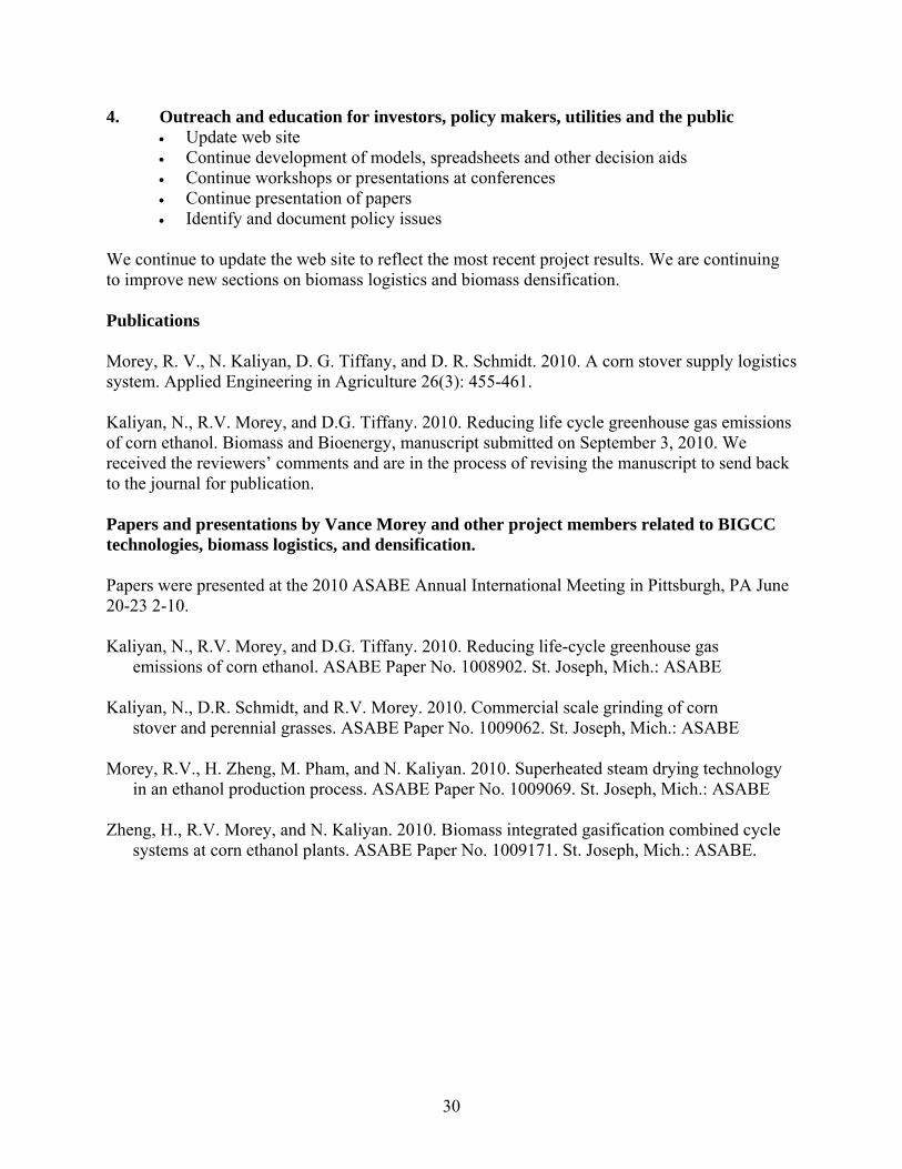
4. Outreach and education for investors, policy makers, utilities and the public • Update web site • Continue development of models, spreadsheets and other decision aids • Continue workshops or presentations at conferences • Continue presentation of papers • Identify and document policy issues

We continue to update the web site to reflect the most recent project results. We are continuing to improve new sections on biomass logistics and biomass densification. Publications Morey, R. V., N. Kaliyan, D. G. Tiffany, and D. R. Schmidt. 2010. A corn stover supply logistics system. Applied Engineering in Agriculture 26(3): 455-461. Kaliyan, N., R.V. Morey, and D.G. Tiffany. 2010. Reducing life cycle greenhouse gas emissions of corn ethanol. Biomass and Bioenergy, manuscript submitted on September 3, 2010. We received the reviewers’ comments and are in the process of revising the manuscript to send back to the journal for publication. Papers and presentations by Vance Morey and other project members related to BIGCC technologies, biomass logistics, and densification. Papers were presented at the 2010 ASABE Annual International Meeting in Pittsburgh, PA June 20-23 2-10. Kaliyan, N., R.V. Morey, and D.G. Tiffany. 2010. Reducing life-cycle greenhouse gas

emissions of corn ethanol. ASABE Paper No. 1008902. St. Joseph, Mich.: ASABE Kaliyan, N., D.R. Schmidt, and R.V. Morey. 2010. Commercial scale grinding of corn

stover and perennial grasses. ASABE Paper No. 1009062. St. Joseph, Mich.: ASABE Morey, R.V., H. Zheng, M. Pham, and N. Kaliyan. 2010. Superheated steam drying technology

in an ethanol production process. ASABE Paper No. 1009069. St. Joseph, Mich.: ASABE Zheng, H., R.V. Morey, and N. Kaliyan. 2010. Biomass integrated gasification combined cycle

systems at corn ethanol plants. ASABE Paper No. 1009171. St. Joseph, Mich.: ASABE.

31

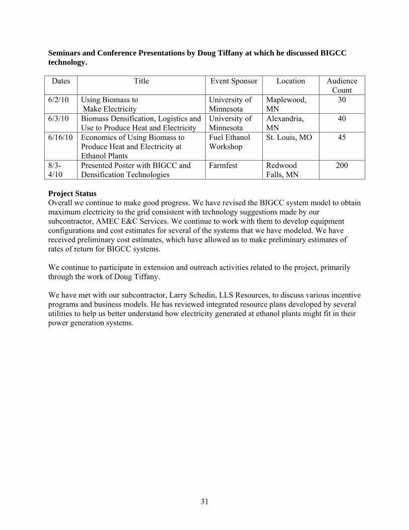
Seminars and Conference Presentations by Doug Tiffany at which he discussed BIGCC technology. Dates Title Event Sponsor Location Audience

Count 6/2/10 Using Biomass to

Make Electricity University of Minnesota

Maplewood, MN

30

6/3/10 Biomass Densification, Logistics and Use to Produce Heat and Electricity

University of Minnesota

Alexandria, MN

40

6/16/10 Economics of Using Biomass to Produce Heat and Electricity at Ethanol Plants

Fuel Ethanol Workshop

St. Louis, MO 45

8/3-4/10

Presented Poster with BIGCC and Densification Technologies

Farmfest Redwood Falls, MN

200

Project Status Overall we continue to make good progress. We have revised the BIGCC system model to obtain maximum electricity to the grid consistent with technology suggestions made by our subcontractor, AMEC E&C Services. We continue to work with them to develop equipment configurations and cost estimates for several of the systems that we have modeled. We have received preliminary cost estimates, which have allowed us to make preliminary estimates of rates of return for BIGCC systems. We continue to participate in extension and outreach activities related to the project, primarily through the work of Doug Tiffany. We have met with our subcontractor, Larry Schedin, LLS Resources, to discuss various incentive programs and business models. He has reviewed integrated resource plans developed by several utilities to help us better understand how electricity generated at ethanol plants might fit in their power generation systems.

biomass electricity generation at ethanol plants - achieving … · 2018-03-27 · system...

Documents