an introduction to the numerics of flow in porous media ... · an introduction to the numerics of...
TRANSCRIPT
An Introduction to the Numerics of Flow inPorous Media using Matlab
Jørg E. Aarnes, Tore Gimse, and Knut–Andreas Lie
SINTEF ICT, Dept. of Applied Mathematics, Oslo
Summary. Even though the art of reservoir simulation has evolved through morethan four decades, there is still a substantial research activity that aims towardfaster, more robust, and more accurate reservoir simulators. Here we attempt togive the reader an introduction to the mathematics and the numerics behind reser-voir simulation. We assume that the reader has a basic mathematical backgroundat the undergraduate level and is acquainted with numerical methods, but no priorknowledge of the mathematics or physics that govern the reservoir flow process isneeded. To give the reader an intuitive understanding of the equations that modelfiltration through porous media, we start with incompressible single-phase flow andmove step-by-step to the black-oil model and compressible two-phase flow. For eachcase, we present a basic numerical scheme in detail, before we discuss a few alter-native schemes that reflect trends in state-of-the-art reservoir simulation. Two andthree-dimensional test cases are presented and discussed. Finally, for the most basicmethods we include simple Matlab codes so that the reader can easily implementand become familiar with the basics of reservoir simulation.
1 Introduction
For nearly half a century, reservoir simulation has been an integrated partof oil-reservoir management. Today, simulations are used to estimate pro-duction characteristics, calibrate reservoir parameters, visualise reservoir flowpatterns, etc. The main purpose is to provide an information database thatcan help the oil companies to position and manage wells and well trajectoriesin order to maximise the oil and gas recovery. Unfortunately, obtaining anaccurate prediction of reservoir flow scenarios is a difficult task. One of thereasons is that we can never get a complete and accurate characterization ofthe rock parameters that influence the flow pattern. And even if we did, wewould not be able to run simulations that exploit all available information,since this would require a tremendous amount of computer resources thatexceed by far the capabilities of modern multi-processor computers. On theother hand, we do not need, nor do we seek a simultaneous description of the

2 Aarnes, Gimse, and Lie
flow scenario on all scales down to the pore scale. For reservoir management itis usually sufficient to describe the general trends in the reservoir flow pattern.
In the early days of the computer, reservoir simulation models were builtfrom two-dimensional slices with 102 − 103 grid cells representing the wholereservoir. In contrast, reservoir characterizations today model the porous rockformations by the means of grid-blocks down to the meter scale. This givesthree-dimensional models consisting of multi-million cells. Despite an aston-ishing increase in computer power, and intensive research on computationtechniques, commercial reservoir simulators can seldom run simulations di-rectly on geological grid models. Instead, coarse grid models with grid-blocksthat are typically ten to hundred times larger are built using some kind ofupscaling of the geophysical parameters. How one should perform this upscal-ing is not trivial. In fact, upscaling has been, and probably still is, one of themost active research areas in the oil industry (see e.g., [7, 13, 14, 31]). Thiseffort reflects that it is a general opinion that, with the ever increasing sizeand complexity of the geological reservoir models, we cannot run simulationsdirectly on these models in the foreseeable future.
Along with the development of better computers, new and more robustupscaling techniques, and more detailed reservoir characterizations, there hasalso been an equally significant development in the area of numerical methods.State-of-the-art simulators employ numerical methods that can take advan-tage of multiple processors, distributed memory workstations, adaptive gridrefinement strategies, and iterative techniques with linear complexity. For thesimulation, there exists a catalogue of different numerical schemes that allhave their pros and cons. With all these techniques available we see a trendwhere methods are being tuned to a special set of applications, as opposed totraditional methods that were developed for a large class of differential equa-tions. As an example, we mention the recent multiscale numerical methods[4, 5, 12, 18, 19, 24] that are specially suited for differential equations whosesolutions may display a multiple scale structure. Although these methods re-semble numerical schemes obtained from an upscaling procedure, they aresomewhat more rigorous in the sense that they exploit fine-scale informationin a mathematically more consistent manner.
It is possible that multiscale methods can help bridge the gap betweenthe size of the geological grid and the size of the simulation grid in reservoirsimulation. This type of contribution would certainly take reservoir simula-tion a big leap forward, and could simplify reservoir management workflowconsiderably. However, although upscaling is undoubtedly an important partof reservoir simulation technology, neither upscaling nor multiscale techniqueswill be discussed here. This part of the reservoir simulation framework is dis-cussed separately elsewhere in this book [1]. Here our purpose is to presenta self-contained tutorial on reservoir simulation. The main idea is to let thereader become familiar with the mathematics behind porous media flow sim-ulation, and present some basic numerical schemes that can be used to solvethe governing partial differential equations. Moreover, to ease the transition

An Introduction to the Numerics of Flow in Porous Media using Matlab 3
from theory to implementation, we supply compact Matlab codes for some ofthe presented methods applied to Cartesian grids. We hope that this materialcan give students or researchers about to embark on, for instance, a Masterproject or a PhD project, a head start.
We assume that the reader has knowledge of mathematics and numericsat the undergraduate level in applied mathematics, but we do not assumeany prior knowledge of reservoir simulation. We therefore start by giving acrash course on the physics and mechanics behind reservoir simulation in Sec-tion 2. This section presents and explains the role of the various geophysicalparameters and indicates how they are obtained. In Section 3 we present thebasic mathematical model in its simplest form: the single-phase flow modelgiving an equation for the fluid pressure. Here we also present some numericalschemes for solving the pressure equation. Then, in Section 4 we move on tomultiphase flow simulation. Multiphase flows give rise to a coupled systemconsisting of a (nearly) elliptic pressure equation and a set of (nearly) hyper-bolic mass transport equations, so-called saturation equations. To balance allterms in these equations properly is a difficult task, and requires quite a bitof bookkeeping. Therefore, to enhance readability, we make some simplifyingassumptions before we start to discretise the equations. Section 5 is thereforedevoted to immiscible two-phase flow where gas is allowed to be dissolved inthe oleic phase. These assumptions give rise to what is known as the black-oilmodel. We then show how to discretise both the pressure equation and thesaturation equations separately, and explain how to deal with the coupling be-tween the pressure equation and the saturation equations. Finally, in Section6, we make some additional assumptions and present a Matlab code for a fulltwo-phase flow simulator. For illustration purposes, the simulator is appliedto some two-dimensional test-cases extracted from a strongly heterogeneousreservoir model that was used as a benchmark for upscaling techniques [13].
2 A Crash Course on the Physics and Mechanics behindReservoir Simulation
The purpose of this section is to briefly summarise some aspects of the art ofmodelling porous media flow and motivate a more detailed study on some ofthe related topics. More details can be found in one of the general textbooksdescribing modelling of flow in porous media, e.g., [6, 11, 15, 20, 27, 29, 33].
Over a period of millions of years, layers of sediments containing organicmaterial built up in the area that is now below the North Sea. A few centime-tres every hundred years piled up to hundreds and thousands of meters andmade the pressure and temperature increase. Simultaneously, severe geolog-ical activity took place. Cracking of continental plates and volcanic activitychanged the area from being a relatively smooth, layered plate into a com-plex structure where previously continuous layers were cut, shifted, or twistedin various directions. As the organic material was compressed, it eventually

4 Aarnes, Gimse, and Lie
turned into a number of different hydrocarbons. Gravity separated trappedwater and the hydrocarbon components. The lightest hydrocarbons (methane,ethane, etc.) usually escaped quickly, whilst the heavier oils moved slowly to-wards the surface. At certain cites, however, the geological activity had createdand bent layers of low-permeable (or non-permeable) rock, so that the migrat-ing hydrocarbons were trapped. These are today’s oil and gas reservoirs in theNorth Sea, and they are typically found at about 1 000–3 000 meters belowthe sea bed.
Although we speak about a porous medium, we should remember it issolid rock. However, almost any naturally formed rock contains pores, andthe distribution and volume fraction of such pores determine the rock proper-ties, which in turn are the parameters governing the hydrocarbon flow in thereservoir.
2.1 Porosity
The rock porosity, usually denoted by φ, is the void volume fraction of themedium, that is, 0 ≤ φ < 1. The porosity usually depends on the pressure;the rock is compressible, and the rock compressibility is defined by:
cr =1φ
dφ
dp, (1)
where p is the overall reservoir pressure. For simplified models, it is customaryto neglect the rock compressibility and assume that φ only depends on thespatial coordinate. If compressibility cannot be neglected, it is common to usea linearization so that:
φ = φ0
(1 + cr(p− p0)
). (2)
For a North Sea reservoir, φ is typically in the range 0.1–0.3, and com-pressibility can be significant, as e.g., witnessed by the subsidence in theEkofisk area. Since the dimension of the pores is very small compared to anyinteresting scale for reservoir simulation, one normally assumes that porosityis a piecewise continuous spatial function. However, ongoing research aimsto understand better the relation between flow models on pore scale and onreservoir scale.
2.2 Permeability
The (absolute) permeability, denoted by K, is a measure of the rock’s abilityto transmit a single fluid at certain conditions. Since the orientation and in-terconnection of the pores are essential for flow, the permeability is not neces-sarily proportional to the porosity, but K is normally strongly correlated to φ.Rock formations like sandstones tend to have many large or well-connectedpores and therefore transmit fluids readily. They are therefore described as

An Introduction to the Numerics of Flow in Porous Media using Matlab 5
permeable. Other formations, like shales, may have smaller, fewer or less in-terconnected pores and are hence described as impermeable. Although theSI-unit for permeability is m2, it is commonly represented in Darcy (D), ormilli-Darcy (mD). The precise definition of 1D (≈ 0.987 · 10−12 m2) involvestransmission of a 1cp fluid (see below) through a homogeneous rock at a speedof 1cm/s due to a pressure gradient of 1atm/cm. Translated to reservoir con-ditions, 1D is a relatively high permeability.
In general, K is a tensor, which means that the permeability in the differentdirections depends on the permeability in the other directions. However, by achange of basis, K may sometimes be diagonalised, and due to the reservoirstructure, horizontal and vertical permeability suffices for several models. Wesay that the medium is isotropic (as opposed to anisotropic) if K can berepresented as a scalar function, e.g., if the horizontal permeability is equalto the vertical permeability. Moreover, due to transitions between differentrock formations, the permeability may vary rapidly over several orders ofmagnitude, local variations in the range 1 mD to 10 D are not unusual in atypical field.
Production (or measurements) may also change the permeability. Whentemperature and pressure is changed, microfractures may open and signifi-cantly change the permeability. Furthermore, since the definition of perme-ability involves a certain fluid, different fluids will experience different per-meability in the same rock sample. Such rock-fluid interactions are discussedbelow.
2.3 Fluid Properties
The void in the porous medium is assumed to be filled with the differentphases. The volume fraction occupied by each phase is the saturation (s) ofthat phase. Thus, ∑
all phases
si = 1. (3)
For practical reservoir purposes, usually only three phases are considered;aqueous (w), oleic (o), and gaseous (g) phase. Each phase contains one ormore components. A hydrocarbon component is a unique chemical species(methan, ethane, propane, etc). Since the number of hydrocarbon compo-nents can be quite large, it is common to group components into psuedo-components. Henceforth we will make no distinction between components andpseudo-components.
Due to the varying and extreme conditions in a reservoir, the hydrocar-bon composition of the different phases may change throughout a simulation(and may sometimes be difficult to determine uniquely). The mass fractionof component i in phase j is denoted by cij . In each of the phases, the massfractions should add up to unity, so that for N different components, we have:
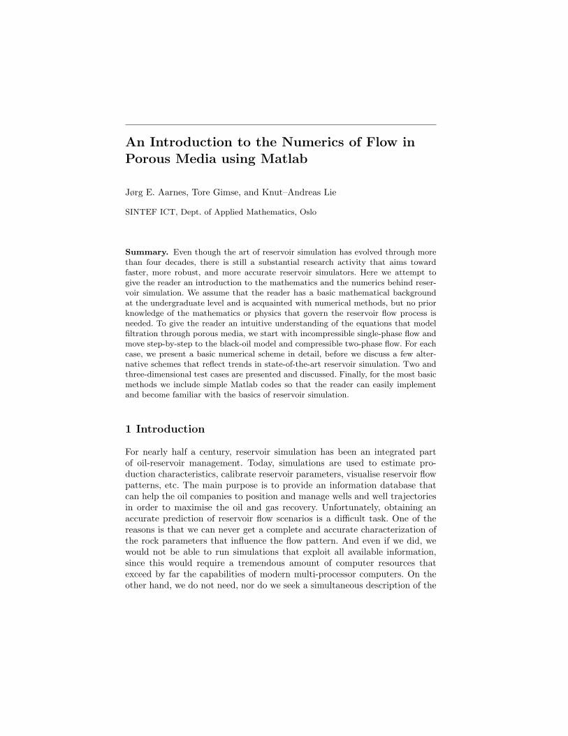
6 Aarnes, Gimse, and Lie
N∑i=1
cig =N∑
i=1
cio =N∑
i=1
ciw = 1. (4)
Next we assign a density ρ and a viscosity µ to each phase. In general,these are functions of phase pressure pi (i = g, o, w) and the composition ofeach phase. That is, for gas
ρg = ρg(pg, c1g, ..., cNg), µg = µg(pg, c1g, ..., cNg), (5)
and similarly for the other phases. These dependencies are most importantfor the gas phase, and are usually ignored for the water phase.
The compressibility of the phase is defined as for rock compressibility:
ci =1ρi
dρi
dpi, i = g, o, w. (6)
Compressibility effects are more important for gas than for oil and water. Insimplified models, water compressibility is therefore usually neglected.
Due to interfacial tensions, the phase pressures are different, defining thecapillary pressure,
pcij = pi − pj , (7)
for i, j = g, o, w. Although other dependencies are reported, it is usually as-sumed that the capillary pressure is a function of the saturations only.
Other parameters of importance are the bubble-point pressures for thevarious components. At given temperature, the bubble-point pressures signifythe pressures where the respective phases start to boil. Below the bubble-pointpressures, gas is released and we get transition of the components between thephases. For most realistic models, even if we do not distinguish between all thecomponents, one allows gas to be dissolved in oil. For such models, an impor-tant pressure-dependent parameter is the solution gas-oil ratio Rs for the gasdissolved in oil at reservoir conditions. It is also common to introduce so-calledformation volume factors (Bw, Bo, Bg) that model the pressure dependent ra-tio of bulk volumes at reservoir and surface conditions. Thermodynamicalbehaviour is, however, a very complex topic that is usually significantly sim-plified or even ignored in reservoir simulation. Thermodynamics will thereforenot be discussed any further here.
2.4 Relative Permeabilities
Even though phases do not really mix, for macroscale modelling, we assumethat all phases may be present at the same location. Thus, it turns out thatthe ability of one phase to move depends on the environment at the actuallocation. That is, the permeability experienced by one phase depends on thesaturation of the other phases at that specific location, as well as the phases’interaction with the pore walls. Thus, we introduce a property called relative

An Introduction to the Numerics of Flow in Porous Media using Matlab 7
permeability, denoted by kri, i = g, o, w, which describes how one phase flowsin the presence of the two others. Thus, in general, and by the closure relation(3), we may assume that
kri = kri(sg, so), (8)
where subscript r stands for relative and i denotes one of the phases g, o, orw. Thus, the (effective) permeability experienced by phase i is Ki = Kkri. Itis important to note that the relative permeabilities are nonlinear functionsof the saturations, so that the sum of the relative permeabilities at a specificlocation (with a specific composition) is not necessarily equal to one. In gen-eral, relative permeabilities may depend on the pore-size distribution, the fluidviscosity, and the interfacial forces between the fluids. These features, whichare carefully reviewed by Demond and Roberts [17], are usually ignored. Ofgreater importance to oil recovery is probably the temperature dependency[28], which may be significant, but very case-related.
Another effect is that due to the adsorption at pore walls and creation ofisolated, captured droplets, the relative permeability curves do not extend allover the interval [0, 1]. The smallest saturation where a phase is mobile is calledthe residual saturation. The adsorption effects may vary, and this may haveimportant effects. Particularly for simulation of polymer injection, adsorptionwill occur and have significant impact on the results. The adsorption of acomponent is usually a nonlinear function, assumed to depend on the rockmatrix, and the concentration of the actual component. Microscopic rock-fluid interactions also imply that the rock absolute permeability is not a well-defined property. Liquids obey no-slip boundary conditions, whilst gases maynot experience the same effects (Klinkenberg effect).
Obtaining measurements of the quantities discussed above, is very difficult.Particularly the relative permeability measurements are costly and trouble-some [23]. Recently, the laboratory techniques have made great progress byusing computer tomography and nuclear magnetic resonance (NMR) to scanthe test cores where the actual phases are being displaced. Although standardexperimental procedures exist for measuring two-phase relative permeabilities(systems where only two phases are present), there is still usually a significantuncertainty concerning the relevance of the experimental values found andit is difficult to come up with reliable data to be used in a simulator. Thisis mainly due to boundary effects. Particularly for three-phase systems, noreliable experimental technique exists. Thus, three-phase relative permeabil-ities are usually modelled using two-phase measurements, for which severaltheoretical models have been proposed. Most of them are based on Stone’smodel [32], where sets of two-phase relative permeabilities are combined togive three-phase data [16]. Recently, a mathematically more plausible modelhas been proposed [25, 26] for the case with no gravity (or with gravity andno counter-current flow). Contrary to the Stone models, the latter exhibits noelliptic regions for the resulting conservation laws.

8 Aarnes, Gimse, and Lie
The uncertainty regarding relative permeability is, however, modest com-pared to the uncertainty imposed by the sparsity of absolute permeabilitydata. To measure K, core samples from the rock are used. These may beabout 10 cm in diameter, taken from vertical test wells at every 25 cm ofdepth. Clearly these samples have negligible volume compared to the entireoil reservoir extending over several kilometres. From outcrops and mines it isknown that rock permeability may vary widely, indicating that the modellingof permeability for a reservoir based on core samples is a tremendously difficultproblem. Some additional information may be gained from seismic measure-ments, but with the technology available today, only large scale structuresmay be found by this technique. Therefore, we have very limited informationabout how the subsurface reservoirs look like. To meet this problem, stochas-tic methods have been applied extensively in the field of reservoir descrip-tion; see Haldorsen and MacDonald [22] and the references therein. Moreover,when comparing and adjusting parameters as real-life production starts, per-meability models can be tuned to fit the actual production data, and therebyhopefully improve the original models and predict future production better.Such approaches are called history matching.
2.5 Production Processes
Initially, a hydrocarbon reservoir is at equilibrium, and contains gas, oil, andwater, separated by gravity. This equilibrium has been established over mil-lions of years with gravitational separation and geological and geothermalprocesses. When a well is drilled through the upper non-permeable layer andpenetrates the upper hydrocarbon cap, this equilibrium is immediately dis-turbed. The reservoir is usually connected to the the well and surface produc-tion facilities by a set of valves. If there were no production valves to stop theflow, we would have a “blow out” since the reservoir is usually under a highpressure. As the well is ready to produce, the valves are opened slightly, andhydrocarbons flow out of the reservoir due to over-pressure. This in turn, setsup a flow inside the reservoir and hydrocarbons flow towards the well, which inturn may induce gravitational instabilities. Also the capillary pressures willact as a (minor) driving mechanism, resulting in local perturbations of thesituation.
During the above process, perhaps 20 percent of the hydrocarbons presentare produced until a new equilibrium is achieved. We call this primary produc-tion by natural drives. One should note that a sudden drop in pressure alsomay have numerous other intrinsic effects. Particularly in complex, compositesystems this may be the case, as pressure-dependent parameters experiencesuch drops. This may give non-convective transport and phase transfers, asvapour and gaseous hydrocarbons may suddenly condensate.
As pressure drops, less oil and gas is flowing, and eventually the produc-tion is no longer economically sustainable. Then the operating company maystart secondary production, by engineered drives. These are processes based on

An Introduction to the Numerics of Flow in Porous Media using Matlab 9
injecting water or gas into the reservoir. The reason for doing this is twofold;some of the pressure is rebuilt or even increased, and secondly one tries to pushout more profitable hydrocarbons with the injected substance. One may per-haps produce another 20 percent of the oil by such processes, and engineereddrives are standard procedure at most locations in the North Sea today.
In order to produce even more oil, Enhanced Oil Recovery (EOR, or ter-tiary recovery) techniques may be employed. Among these are heating thereservoir or injection of sophisticated substances like foam, polymers or sol-vents. Polymers are supposed to change the flow properties of water, andthereby to more efficiently push out oil. Similarly, solvents change the flowproperties of the hydrocarbons, for instance by developing miscibility withan injected gas. In some sense, one tries to wash the pore walls for most ofthe remaining hydrocarbons. The other technique is based on injecting steam,which will heat the rock matrix, and thereby, hopefully, change the flow prop-erties of the hydrocarbons. At present, such EOR techniques are consideredtoo expensive for large scale commercial use, but several studies have beenconducted and the mathematical foundations are being carefully investigated,and at smaller scales EOR is being performed.
One should note that the terms primary, secondary, and tertiary are am-biguous. EOR techniques may be applied during primary production, andsecondary production may be performed from the first day of production.
3 Incompressible Single-Phase Flow
The simplest possible way to describe the displacements of fluids in a reser-voir is by a single-phase model. This model gives an equation for the pressuredistribution in the reservoir and is used for many early-stage and simplifiedflow studies. Single-phase models are used to identify flow directions; iden-tify connections between producers and injectors; in flow-based upscaling; inhistory matching; and in preliminary model studies.
3.1 Basic Model
Assume that we want to model the filtration of a fluid through a porousmedium of some kind. The basic equation describing this process is the con-tinuity equation which states that mass is conserved
∂(φρ)∂t
+∇ · (ρv) = q. (9)
Here the source term q models sources and sinks, that is, outflow and inflowper volume at designated well locations.
For low flow velocities v, filtration through porous media is modelled withan empirical relation called Darcy’s law after the French engineer Henri Darcy.

10 Aarnes, Gimse, and Lie
Darcy discovered in 1856, through a series of experiments, that the filtrationvelocity is proportional to a combination of the gradient of the fluid pressureand pull-down effects due to gravity. More precisely, the volumetric flow den-sity v (which we henceforth will refer to as flow velocity) is related to pressurep and gravity forces through the following gradient law:
v = −Kµ
(∇p+ ρg∇z). (10)
Here K is the permeability, µ is the viscosity, g is the gravitational constantand z is the spatial coordinate in the upward vertical direction. For brevity weshall in the following write G = −g∇z for the gravitational pull-down force.
In most real field geological reservoir models, K is an anisotropic diagonaltensor. Unfortunately, as mentioned in the introduction, commercial reservoirsimulators can seldom run simulations directly on these geological models.Effects of small-scale heterogeneous structures are therefore incorporated intosimulation models by designing effective permeability tensors that representimpact of small-scale heterogeneous structures on a coarser grid, as discussedin more detail elsewhere in this book [1]. These effective, or upscaled, per-meability tensors try to model principal flow directions, which may not bealigned with the spatial coordinate directions, and can therefore be full ten-sors. Hence, here we assume only that K is a symmetric and positive definitetensor, whose eigenvalues are bounded uniformly below and above by positiveconstants.
We note that Darcy’s law is analogous to Fourier’s law of heat conduction(in which K is replaced with the heat conductivity tensor) and Ohm’s law ofelectrical conduction (in which K is the inverse of the electrical resistance).However, whereas there is only one driving force in thermal and electricalconduction, there are two driving forces in porous media flow: gravity andthe pressure gradient. Since gravity forces are approximately constant insidea reservoir domain Ω, we need only use the reservoir field pressure as ourprimary unknown. To solve for the pressure, we combine Darcy’s law (10)with the continuity equation (9).
To illustrate, we derive an equation that models flow of a fluid, say, water(w), through a porous medium characterised by a permeability field K and acorresponding porosity distribution. For simplicity, we assume that the poros-ity φ is constant in time and that the flow can be adequately modelled byassuming incompressibility, i.e., constant density. Then the temporal deriva-tive term in (9) vanishes and we obtain the following elliptic equation for thewater pressure:
∇ · vw = ∇ ·[− Kµw
(∇pw − ρwG)]
=qwρw. (11)
To close the model, we must specify boundary conditions. Unless stated oth-erwise we shall follow common practice and use no-flow boundary conditions.

An Introduction to the Numerics of Flow in Porous Media using Matlab 11
Hence, on the reservoir boundary ∂Ω we impose vw · n = 0, where n is thenormal vector pointing out of the boundary ∂Ω. This gives us an isolated flowsystem where no water can enter or exit the reservoir.
In the next subsections we restrict our attention to incompressible flowsand present several numerical methods for solving (11). To help the interestedreader with the transition from theory to implementation, we also discusssome simple implementations in Matlab for uniform Cartesian grids. We firstpresent a cell-centred finite-volume method, which is sometimes referred toas the two-point flux-approximation (TPFA) scheme. Although this schemeis undoubtedly one of the simplest discretisation techniques for elliptic equa-tions, it is still widely used in the oil-industry.
3.2 A Simple Finite-Volume Method
In classical finite-difference methods, partial differential equations (PDEs) areapproximated by replacing the partial derivatives with appropriate divideddifferences between point-values on a discrete set of points in the domain.Finite-volume methods, on the other hand, have a more physical motivationand are derived from conservation of (physical) quantities over cell volumes.Thus, in a finite-volume method the unknown functions are represented interms of average values over a set of finite-volumes, over which the integratedPDE model is required to hold in an averaged sense.
Although finite-difference and finite-volume methods have fundamentallydifferent interpretation and derivation, the two labels are used interchangeablyin the scientific literature. We therefore choose to not make a clear distinc-tion between the two discretisation techniques here. Instead we ask the readerto think of a finite-volume method as a conservative finite-difference schemethat treats the grid cells as control volumes. In fact, there exist several finite-volume and finite-difference schemes of low order, for which the cell-centredvalues obtained with the finite-difference schemes coincide with cell averagesobtained with the corresponding finite-volume schemes. The two representa-tions of the unknown functions will therefore also be used interchangeablyhenceforth.
To derive a set of finite-volume mass-balance equations for (11), denote byΩi a grid cell in Ω and consider the following integral over Ωi:∫
Ωi
( qwρw
−∇ · vw
)dx = 0. (12)
Invoking the divergence theorem, assuming that vw is sufficiently smooth,equation (12) transforms into the following mass-balance equation:∫
∂Ωi
vw · n dν =∫
Ωi
qwρw
dx. (13)
Here n denotes the outward-pointing unit normal on ∂Ωi. Correspondingfinite-volume methods are now obtained by approximating the pressure pw

12 Aarnes, Gimse, and Lie
with a cell-wise constant function pw = pw,i and estimating vw · n acrosscell interfaces γij = ∂Ωi ∩ ∂Ωj from a set of neighbouring cell pressures.
To formulate the standard two-point flux-approximation (TPFA) finite-volume scheme that is frequently used in reservoir simulation, it is convenientto reformulate equation (11) slightly, so that we get an equation on the form
−∇ · λ∇u = f, (14)
where λ = K/µw. To this end, we have two options: we can either introducea flow potential uw = pw +ρwgz and express our model as an equation for uw
−∇ · λ∇uw =qwρw,
or we can move the gravity term ∇ · (λρwG) to the right-hand side. Hence,we might as well assume that we want to solve equation (14) for u.
As the name suggests, the TPFA scheme uses two points, the cell-averagesui and uj , to approximate the flux vij = −
∫γij
(λ∇u) · n dν. To be morespecific, let us consider a regular hexahedral grid with gridlines aligned withthe principal coordinate axes. Moreover, assume that γij is an interface be-tween adjacent cells in the x–coordinate direction so that nij = (1, 0, 0)T . Thegradient ∇u on γij in the TPFA method is now replaced with
δuij =2(uj − ui)∆xi +∆xj
, (15)
where ∆xi and ∆xj denote the respective cell dimensions in the x-coordinatedirection. Thus, we obtain the following expression for vij :
vij = δuij
∫γij
λdν =2(uj − ui)∆xi +∆xj
∫γij
λdν.
However, in most reservoir simulation models, the permeability K is cell-wiseconstant, and hence not well-defined at the interfaces. This means that wealso have to approximate λ on γij . In the TPFA method this is done bytaking a distance-weighted harmonic average of the respective directional cellpermeabilities, λi,ij = nij · λinij and λj,ij = nij · λjnij . To be precise, thenij–directional permeability λij on γij is computed as follows:
λij = (∆xi +∆xj)(∆xi
λi,ij+∆xj
λj,ij
)−1
,
Hence, for orthogonal grids with gridlines aligned with the coordinate axes,one approximates the flux vij in the TPFA method in the following way:
vij = −|γij |λijδuij = 2|γij |(∆xi
λi,ij+∆xj
λj,ij
)−1
(ui − uj). (16)

An Introduction to the Numerics of Flow in Porous Media using Matlab 13
Finally, summing over all interfaces to adjacent cells, we get an approximationto
∫∂Ωi
vw · n dν, and the associated TPFA method is obtained by requiringthe mass balance equation (13) to be fulfilled for each grid cell Ωi ∈ Ω.
In the literature on finite-volume methods it is common to express theflux vij in a more compact form than we have done in (16). Terms thatdo not involve the cell potentials ui are usually gathered into an interfacetransmissibility tij . For the current TPFA method the transmissibilities aredefined by:
tij = 2|γij |(∆xi
λi,ij+∆xj
λj,ij
)−1
.
Thus by inserting the expression for tij into (16), we see that the TPFAscheme for equation (14), in compact form, seeks a cell-wise constant functionu = ui that satisfies the following system of equations:∑
j
tij(ui − uj) =∫
Ωi
f dx, ∀Ωi ⊂ Ω, (17)
This system is clearly symmetric, and a solution is, as for the continuousproblem, defined up to an arbitrary constant. The system is made positivedefinite, and symmetry is preserved, by forcing u1 = 0, for instance. That is,by adding a positive constant to the first diagonal of the matrix A = [aik],where:
aik =∑
j tij if k = i,
−tik if k 6= i,
The matrix A is sparse, consisting of a tridiagonal part corresponding to thex-derivative, and two off-diagonal bands corresponding to the y-derivatives.
A short Matlab code for the implementation of (17) on a uniform Carte-sian grid is given in Listing 1. In a general code, one would typically assemblethe coefficient matrix by looping over all the interfaces of each grid block andfor each interface, compute the associated transmissibilities and add them intothe correct position of the system matrix. Similarly, the interface fluxes wouldbe computed by looping over all grid block interfaces. Such an approach wouldeasily be extensible to other discretisation (e.g., the MPFA method discussedin the next section) and to more complex grids (e.g., unstructured and faultedgrids). Our code has instead been designed to be compact and efficient, andtherefore relies entirely on the Cartesian grid structure to set up the trans-missibilities in the coefficient matrix using Matlab’s inherent vectorization.
In the code, K is a 3×Nx×Ny×Nz matrix holding the three diagonals of thetensor λ for each grid cell. The coefficient matrix A is sparse (use e.g., spy(A)to visualise the sparsity pattern) and is therefore generated with Matlab’sbuilt-in sparse matrix functions. Understanding the Matlab code should berather straightforward. The only point worth noting is perhaps that the con-stant that we use to force u1 = 0 in element A(1,1) is taken as the sum ofthe diagonals in λ. This is done in order to control that this extra equationdoes not have an adverse effect on the condition number of A.

14 Aarnes, Gimse, and Lie
Listing 1. TPFA finite-volume discretisation of −∇(K(x)∇u) = q.
function [P,V]=TPFA(Grid,K,q)
% Compute transmissibilities by harmonic averaging.Nx=Grid.Nx; Ny=Grid.Ny; Nz=Grid.Nz; N=Nx∗Ny∗Nz;hx=Grid.hx; hy=Grid.hy; hz=Grid.hz;L = K.ˆ(−1);tx = 2∗hy∗hz/hx; TX = zeros(Nx+1,Ny,Nz);ty = 2∗hx∗hz/hy; TY = zeros(Nx,Ny+1,Nz);tz = 2∗hx∗hy/hz; TZ = zeros(Nx,Ny,Nz+1);TX(2:Nx,:,:) = tx./(L(1,1:Nx−1,:,:)+L(1,2:Nx ,:,:));TY(:,2:Ny,:) = ty./(L (2,:,1: Ny−1,:)+L(2,:,2:Ny,:));TZ (:,:,2: Nz) = tz./(L (3,:,:,1: Nz−1)+L(3,:,:,2:Nz));
% Assemble TPFA discretization matrix.x1 = reshape(TX(1:Nx,:,:),N,1); x2 = reshape(TX(2:Nx+1,:,:),N,1);y1 = reshape(TY(:,1:Ny,:),N,1); y2 = reshape(TY(:,2:Ny+1,:),N,1);z1 = reshape(TZ(:,:,1:Nz),N,1); z2 = reshape(TZ(:,:,2:Nz+1),N,1);DiagVecs = [−z2,−y2,−x2,x1+x2+y1+y2+z1+z2,−x1,−y1,−z1];DiagIndx = [−Nx∗Ny,−Nx,−1,0,1,Nx,Nx∗Ny];A = spdiags(DiagVecs,DiagIndx,N,N);A(1,1) = A(1,1)+sum(Grid.K(:,1,1,1));
% Solve linear system and extract interface fluxes.u = A\q;P = reshape(u,Nx,Ny,Nz);V.x = zeros(Nx+1,Ny,Nz);V.y = zeros(Nx,Ny+1,Nz);V.z = zeros(Nx,Ny,Nz+1);V.x(2:Nx ,:,:) = (P(1:Nx−1,:,:)−P(2:Nx,:,:)).∗TX(2:Nx,:,:);V.y (:,2:Ny,:) = (P(:,1:Ny−1,:)−P(:,2:Ny,:)).∗TY(:,2:Ny,:);V.z (:,:,2: Nz) = (P (:,:,1: Nz−1)−P(:,:,2:Nz)).∗TZ(:,:,2:Nz);
Example 1. In the first example we consider a homogeneous and isotropicpermeability K ≡ 1 for all x ∈ IR2. We place an injection well at the originand production wells at the points (±1,±1) and specify no-flow conditionsat the boundaries. These boundary conditions give the same flow as if werepeated the five-spot well pattern to infinity in every direction. The flow inthe five-spot is symmetric about both the coordinate axes. We can thereforereduce the computational domain to a quarter, and use e.g., the unit boxΩ = [0, 1]2. The corresponding problem is called a quarter-five spot problem,and is a standard test-case for numerical methods in reservoir simulation.
Figure 1 shows pressure contours. The pressure P is computed by thefollowing lines for a 8× 8 grid:
>> Grid.Nx=8; Grid.hx=1/Grid.Nx;>> Grid.Ny=8; Grid.hy=1/Grid.Ny;>> Grid.Nz=1; Grid.hz=1/Grid.Nz;>> Grid.K=ones(3,Grid.Nx,Grid.Ny);>> N=Grid.Nx∗Grid.Ny∗Grid.Nz; q=zeros(N,1); q([1 N])=[1 −1];>> P=TPFA(Grid,Grid.K,q);
Here the command P=TPFA(· · · ) assigns to P the first (the local variable U) ofthe four output variables U, FX, FY, and FZ.

An Introduction to the Numerics of Flow in Porous Media using Matlab 15
0 0.1 0.2 0.3 0.4 0.5 0.6 0.7 0.8 0.9 10
0.1
0.2
0.3
0.4
0.5
0.6
0.7
0.8
0.9
1
0.5
1
1.5
2
2.5
5 10 15 20 25 30
5
10
15
20
25
30
−1
−0.5
0
0.5
1
0 0.1 0.2 0.3 0.4 0.5 0.6 0.7 0.8 0.9 10
0.1
0.2
0.3
0.4
0.5
0.6
0.7
0.8
0.9
1
0.5
1
1.5
2
2.5
3
3.5
4
Fig. 1. The left plot shows pressure contours for a homogeneous quarter-five spot.The middle plot shows logarithm of the permeability for the heterogeneous quarter-five spot and the right plot the corresponding pressure distribution. As particles flowin directions of decreasing pressure gradient, the pressure decays from the injectorin the lower-left to the producer in the upper-right corner.
Next we increase the number of grid-cells in each direction from eight to32 and consider a slightly more realistic permeability field obtained from alog-normal distribution.
>> Grid.Nx=32; Grid.hx=1/Grid.Nx;>> Grid.Ny=32; Grid.hy=1/Grid.Ny;>> Grid.Nz=1; Grid.hz=1/Grid.Nz;>> Grid.K=exp(5∗smooth3(smooth3(randn(3,Grid.Nx,Grid.Ny))));>> N=Grid.Nx∗Grid.Ny∗Grid.Nz; q=zeros(N,1); q([1 N])=[1 −1];>> P=TPFA(Grid,Grid.K,q);
The permeability and pressure distribution is plotted in Figure 1.
3.3 Multipoint Flux-Approximation Schemes
The TPFA finite-volume scheme presented above is convergent only if eachgrid cell is a parallelepiped and
nij ·Knik = 0, ∀Ωi ⊂ Ω, nij 6= nik, (18)
where nij and nik denote normal vectors into two neighbouring grid cells. Agrid consisting of parallelepipeds satisfying (18) is said to be K-orthogonal.Orthogonal grids are, for example, K-orthogonal with respect to diagonal per-meability tensors, but not with respect to full tensor permeabilities. Figure 2shows a schematic of an orthogonal grid and a K-orthogonal grid.
If the TPFA method is used to discretise equation (14) on grids that arenot K-orthogonal, the scheme will produce different results depending on theorientation of the grid (so-called grid-orientation effects) and will convergeto a wrong solution. Despite this shortcoming of the TPFA method, it isstill the dominant (and default) method for practical reservoir simulation,owing to its simplicity and computational speed. We present now a class ofso-called multi-point flux-approximation (MPFA) schemes that aim to amendthe shortcomings of the TPFA scheme.

16 Aarnes, Gimse, and Lie
∆j∆i
KjγijiK
nn
12
K
nTKn1 2 =0
Fig. 2. The grid in the left plot is orthogonal with gridlines aligned with the principalcoordinate axes. The grid in the right plot is a K-orthogonal grid.
Consider an orthogonal grid and assume that K is a constant tensor withnonzero off-diagonal terms. Moreover, for presentational simplicity, let γij bean interface between two adjacent grid cells in the x–coordinate direction.Then for a given function u, the corresponding flux across γij is given by:∫
γij
vw · nij dν = −∫
γij
(kxx∂xu+ kxy∂yu+ kxz∂zu
)dν.
This expression involves derivatives in three orthogonal coordinate directions.Evidently, two point values can only be used to estimate a derivative in onedirection. In particular, the two cell averages ui and uj can not be used toestimate the derivative of u in the y and z-directions. Hence, the TPFA schemeneglects the flux contribution from kxy∂yu and kxz∂zu.
To obtain consistent interfacial fluxes for grids that are not K-orthogonal,one must also estimate partial derivatives in coordinate directions parallel tothe interfaces. For this purpose, more than two point values, or cell averages,are needed. This leads to schemes that approximate vij using multiple cellaverages, that is, with a linear expression on the form:
vij =∑
k
tkijgkij(u).
Here tkijk are the transmissibilities associated with γij and gkij(u)k are the
corresponding multi-point pressure or flow potential dependencies. Thus, wesee that MPFA schemes for (14) can be written on the form:∑
j,k
tkijgkij(u) =
∫Ωi
f dx, ∀Ωi ⊂ Ω. (19)
MPFA schemes can, for instance, be designed by simply estimating each of thepartial derivatives ∂ξu from neighbouring cell averages. However, most MPFAschemes have a more physical motivation and are derived by imposing certaincontinuity requirements. We will now outline very briefly one such method,

An Introduction to the Numerics of Flow in Porous Media using Matlab 17
Ω1
Ω2 Ω
3
Ω4
x1
x2 x
3
x4
Ω1II
Ω2IV
Ω3III
Ω4I
x12
x23
x34
x14
Fig. 3. The shaded region represents the interaction region for the O-method on atwo-dimensional quadrilateral grid associated with cells Ω1, Ω2, Ω3, and Ω4.
called the O-method [2, 3], for irregular, quadrilateral, matching grids in twospatial dimensions.
The O-method is constructed by defining an interaction region (IR) aroundeach corner point in the grid. For a two-dimensional quadrilateral grid, thisIR is the area bounded by the lines that connect the cell-centres with themidpoints on the cell interfaces, see Figure 3. Thus, the IR consists of foursub-quadrilaterals (Ωii
1 , Ωiv2 , Ω
iii3 , and Ωi
4) from four neighbouring cells (Ω1,Ω2, Ω3, and Ω4) that share a common corner point. For each IR, define now
Uir = spanU ji : i = 1, . . . , 4, j=i,. . . ,iv,
where U ji are linear functions on the respective four sub-quadrilaterals. With
this definition, Uir has twelve degrees of freedom. Indeed, note that each U ji
can be expressed in the following non-dimensional form
U ji (x) = ui +∇U j
i · (x− xi),
where xi is the cell centre in Ωi. The cell-centre values ui thus account for fourdegrees of freedom and the (constant) gradients ∇UJ
i for additional eight.Next we require that functions in Uir are: (i) continuous at the midpoints of
the cell interfaces, and (ii) flux-continuous across the interface segments thatlie inside the IR. To obtain a globally coupled system, we first use (i) and (ii)to express the gradients ∇UJ
i , and hence also the corresponding fluxes acrossthe IR interface segments, in terms of the unknown cell-centre potentials ui.This requires solution of a local system of equations. Finally, the cell-centrepotentials are determined (up to an arbitrary constant for no-flow bound-ary conditions) by summing the fluxes across all IR interface segments andrequiring that the mass balance equations (13) hold. In this process, transmis-sibilities are assembled to obtain a globally coupled system for the unknownpressures over the whole domain.
We note that this construction leads to an MPFA scheme where the fluxacross an interface γij depends on the potentials uj in a total of six neighbour-

18 Aarnes, Gimse, and Lie
ing cells (eighteen in three dimensions). Notice also that the transmissibilitiestkij that we obtain when eliminating the IR gradients now account for grid-cell geometries in addition to full-tensor permeabilities.
3.4 A Mixed Finite-Element Method
As an alternative to the MPFA schemes, one can use mixed finite-elementmethods (FEMs) [10]. In mixed FEMs, the fluxes over cell edges are consideredas unknowns in addition to the pressures, and are not computed using a(numerical) differentiation as in finite-volume methods. For the mixed FEMsthere is little to gain by reformulating (11) into an equation on the form (14).We therefore return to the original formulation and describe how to discretisethe following system of differential equations with mixed FEMs:
v = −λ(∇p− ρG), ∇ · v = q. (20)
As before we impose no-flow boundary conditions on ∂Ω. To derive the mixedformulation, we first define the following Sobolev space
H1,div0 (Ω) = v ∈ (L2(Ω))d : ∇ · v ∈ L2(Ω) and v · n = 0 on ∂Ω.
The mixed formulation of (20) (with no-flow boundary conditions) now reads:find (p, v) ∈ L2(Ω)×H1,div
0 (Ω) such that∫Ω
v · λ−1u dx−∫
Ω
p ∇ · u dx =∫
Ω
ρG · u dx, (21)∫Ω
l ∇ · v dx =∫
Ω
ql dx, (22)
for all u ∈ H1,div0 (Ω) and l ∈ L2(Ω). We observe again that, since no-flow
boundary conditions are imposed, an extra constraint must be added to make(21)–(22) well-posed. A common choice is to use
∫Ωp dx = 0.
In mixed FEMs, (21)–(22) are discretised by replacing L2(Ω) andH1,div0 (Ω)
with finite-dimensional subspaces U and V , respectively. For instance, in theRaviart–Thomas mixed FEM [30] of lowest order (for triangular, tetrahedral,or regular parallelepiped grids), L2(Ω) is replaced by
U = p ∈ L2(Ω) : p|Ωiis constant ∀Ωi ∈ Ω
and H1,div0 (Ω) is replaced by
V = v ∈ H1,div0 (Ω) : v|Ωi have linear components ∀Ωi ∈ Ω,
(v · nij)|γij is constant ∀γij ∈ Ω, and v · nij is continuous across γij.
Here nij is the unit normal to γij pointing from Ωi to Ωj . The correspondingRaviart–Thomas mixed FEM thus seeks

An Introduction to the Numerics of Flow in Porous Media using Matlab 19
(p, v) ∈ U × V such that (21)–(22) hold for all u ∈ V and q ∈ U. (23)
To express (23) as a linear system, observe first that functions in V are, foradmissible grids, spanned by base functions ψij that are defined by
ψij ∈ P(Ωi)d ∪ P(Ωj)d and (ψij · nkl)|γkl=
1 if γkl = γij ,
0 else,
where P(K) is the set of linear functions on K. Similarly
U = spanχm where χm =
1 if x ∈ Ωm,
0 else.
Thus, writing p =∑
Ωmpmχm and v =
∑γijvijψij , allows us to write (23) as
a linear system in p = pm and v = vij. This system takes the form[B −CT
C 0
] [vp
]=
[gf
]. (24)
Here f = [fm], g = [gkl], B = [bij,kl] and C = [cm,kl], where:
gkl =[∫
Ω
ρG · ψkl dx], fm =
[∫Ωm
f dx],
bij,kl =[∫
Ω
ψij · λ−1ψkl dx], cm,kl =
[∫Ωm
∇ · ψkl dx].
Note that for the current Raviart-Thomas finite elements, we have
cm,kl =
1 if m = k,
−1 if m = l,
0 otherwise.
The matrix entries bij,kl, on the other hand, depend on the geometry of thegrid cells and the form of λ. In other words, the entries depend on whether λis isotropic or anisotropic, whether λ is cell-wise constant or models subgridvariations in the permeability field.
We provide now a Matlab code implementing the Raviart-Thomas mixedFEM for the first-order system (20) on a regular hexahedral grid in three spa-tial dimensions. The code is divided into three parts: assembly of the B block;assembly of the C block; and a main routine that loads data (permeability andgrid), assembles the whole matrix, and solves the system. Again we emphasisecompactness and efficiency, by heavily relying on the Cartesian grid and ana-lytical integration of the Raviart-Thomas basis functions to perform a directassembly of the matrix blocks. For more general grids, one would typicallyperform an elementwise assembly by looping over all grid blocks and replacethe integration over basis functions by some numerical quadrature rule.

20 Aarnes, Gimse, and Lie
Listing 2. Assembly of B for the lowest-order Raviart–Thomas elements.
function B=GenB(Grid,K)
Nx=Grid.Nx; Ny=Grid.Ny; Nz=Grid.Nz; N=Nx∗Ny∗Nz;hx=Grid.hx; hy=Grid.hy; hz=Grid.hz;L = K.ˆ(−1);ex=N−Ny∗Nz; ey=N−Nx∗Nz; ez=N−Nx∗Ny; % Number of edgestx=hx/(6∗hy∗hz); ty=hy/(6∗hx∗hz); tz=hz/(6∗hx∗hy); % Transmissibilities
X1=zeros(Nx−1,Ny,Nz); X2=zeros(Nx−1,Ny,Nz); % Preallocate memoryX0=L(1,1:Nx−1,:,:)+L(1,2:Nx,:,:); x0=2∗tx∗X0(:); % Main diagonalX1(2:Nx−1,:,:)=L(1,2:Nx−1,:,:); x1=tx∗X1(:); % Upper diagonalX2(1:Nx−2,:,:)=L(1,2:Nx−1,:,:); x2=tx∗X2(:); % Lower diagonal
Y1=zeros(Nx,Ny−1,Nz); Y2=zeros(Nx,Ny−1,Nz); % Preallocate memoryY0=L(2,:,1:Ny−1,:)+L(2,:,2:Ny,:); y0=2∗ty∗Y0(:); % Main diagonalY1(:,2:Ny−1,:)=L(2,:,2:Ny−1,:); y1=ty∗Y1(:); % Upper diagonalY2(:,1:Ny−2,:)=L(2,:,2:Ny−1,:); y2=ty∗Y2(:); % Lower diagonal
Lz1=L(3,:,:,1:Nz−1); z1=tz∗Lz1(:); % Upper diagonalLz2=L(3,:,:,2:Nz); z2=tz∗Lz2(:); % Lower diagonalz0=2∗(z1+z2); % Main diagonal
B=[spdiags([x2,x0,x1],[−1,0,1],ex,ex),sparse(ex,ey+ez);...sparse(ey,ex),spdiags([y2,y0,y1],[−Nx,0,Nx],ey,ey),sparse(ey,ez );...sparse(ez,ex+ey),spdiags([z2,z0,z1],[−Nx∗Ny,0,Nx∗Ny],ez,ez)];
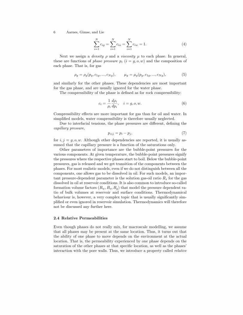
In Listing 2 we show a Matlab function that assembles the B matrix. Hereλ is assumed to be a diagonal tensor and is represented as a 3×Nx×Ny×Nzmatrix K with Nx, Ny, and Nz denoting the number of grid cells in the x, y, andz direction, respectively. The degrees of freedom at the interfaces (the fluxes)have been numbered in the same way as the grid-blocks; i.e., first in the x-direction, then in the y-direction, and finally in the z-direction. This gives B ahepta-diagonal structure as shown in Figure 4, where the three nonzero blockscorrespond to the three components of v. Notice, however, that since the gridis K-orthogonal, we can make B tridiagonal by starting the numbering of eachcomponent of v = (vx, vy, vz) in the corresponding direction; i.e., number vx
as xyz, vy as yxz, and vz as zxy. Similar observations can be made for theassembly of C, which is given in Listing 3.
Let us now make a few brief remarks with respect to the implementation ofthe assembly of the matrix blocks B and C. First, since only a few componentsof B and C are nonzero, we store them using a sparse matrix format. Thematrices are created in a block-wise manner using Matlab’s built in sparsematrix functions. The function sparse(m,n) creates an m × n zero matrixand spdiags(M,d,m,n) creates an m × n sparse matrix with the columns ofM on the diagonals specified by d. Finally, statements of the form M(:) turnthe matrix M into a column vector.
A drawback with the mixed FEM is that it produces an indefinite linearsystem. These systems are in general harder to solve than the positive definitesystems that arise, e.g., from the TPFA and MPFA schemes described in
An Introduction to the Numerics of Flow in Porous Media using Matlab 21
A: B:
C:
Fig. 4. Sparsity patterns for A, B, and C for a case with 4× 3× 3 grid-blocks.
Listing 3. Assembly of C for the lowest-order Raviart–Thomas elements.
function C=GenC(Grid)
Nx=Grid.Nx; Ny=Grid.Ny; Nz=Grid.Nz;C=sparse(0,0); % Empty sparse matrixNxy=Nx∗Ny; N=Nxy∗Nz; % Number of grid−pointsvx=ones(Nx,1); vy=ones(Nxy,1); vz=ones(N,1); % Diagonals
for i=1:Ny∗Nz % vx−block of CCx=spdiags([vx,−vx],[−1,0]−(i−1)∗Nx,N,Nx−1); % create bidiagonal blockC=[C,Cx]; % append to C
end
for i=1:Nz % vy−block of CCy=spdiags([vy,−vy],[−Nx,0]−(i−1)∗Nxy,N,Nxy−Nx); % create bidiagonal blockC=[C,Cy]; % append to C
end
C = [C, spdiags([vz,−vz],[−Nxy,0],N,N−Nxy)]; % vz−block of C
Sections 3.2 and 3.3. In fact, for second-order elliptic equations of the form(11) it is common to use a so-called hybrid formulation. This method leads toa positive definite system where the unknowns correspond to pressures at grid-cell interfaces. The solution to the linear system arising from the mixed FEMcan now be obtained from the solution to the hybrid system by performingonly local algebraic calculations. This property, which is sometimes referredto as explicit flux representation, allows the inter-cell fluxes that appear in thesaturation equation to be expressed as a linear combination of neighbouringvalues for the pressure.

22 Aarnes, Gimse, and Lie
Explicit flux representation is a feature that also the finite-volume methodsenjoy. One of the main advantages is that it allows us to compute fully implicitsolutions without computing the fluxes explicitly. Indeed, in the mixed FEM,which does not have an explicit flux representation, one has to solve the fullindefinite linear system for the pressure equation alongside the linear systemfor the saturation equation in order to produce a fully implicit solution. Wewould like to comment, however, that whether or not a discretisation methodfor the pressure equation allows an explicit flux representation may mostlybe regarded as a minor issue. Indeed, one is always free to use a sequentialimplicit solution strategy which is often faster and in most cases results in thesame, or at least an equally accurate solution.
It is not within our scope here to discuss issues related to solving linearsystems that arise from mixed FEM discretisations further. Indeed, for mod-erately sized problems we can rely on Matlab, and the possibly complex linearalgebra involved in solving the sparse system (24) can be hidden in a simplestatement of the form x = A\b. Readers interested in learning more aboutmixed FEMs, and how to solve the corresponding linear systems are advisedto consult some of the excellent books on the subject, for instance [8, 9, 10].
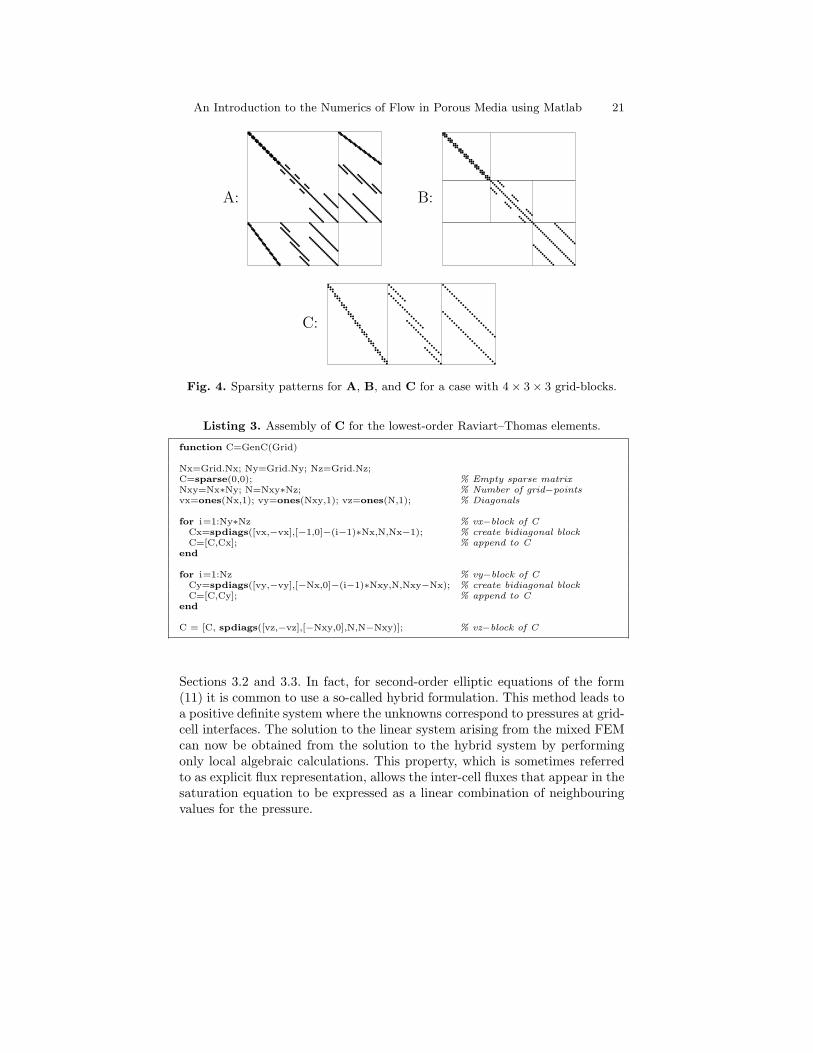
Example 2. It is now time to consider our first reservoir having more thanonly a touch of realism. To this end we will simulate two horizontal slicesof Model 2 from the 10th SPE Comparative Solution Project [13], whichis publicly available on the net. The model dimensions are 1200 × 2200 ×170 (ft) and the reservoir is described by a heterogeneous distribution over aregular Cartesian grid with 60×220×85 grid-blocks. We pick the top layer, inwhich the permeability is smooth, and the bottom layer, which is fluvial andcharacterised by a spaghetti of narrow high-flow channels (see Figure 5). Forboth layers, the permeabilities range over at least six orders of magnitude. Todrive a flow in the two layers, we impose an injection and a production wellin the lower-left and upper-right corners, respectively.
Listing 4 contains a simulation routine that loads data, assembles the wholematrix, and solves the system (24) to compute pressure and fluxes (neglecting,for brevity, gravity forces so that G = 0) . For the flux, only the interior edgesare computed, since the flux normal to the exterior edges is assumed to bezero through the no-flow boundary condition.
In Figure 5 we visualise the flow field using 20 streamlines imposed upona colour plot of the logarithm of the permeability. For completeness, we haveincluded the Matlab code used to generate each of the plots. Some of thestreamlines in the plots seem to appear and disappear at the boundaries.This is a pure plotting artifact obtained when we collocate the staggered edgefluxes at the cell centres in order to use Matlab’s streamline visualisationroutine.
In the next sections we will demonstrate how the models and numericalmethods introduced above for single-phase flow can be extended to more gen-

An Introduction to the Numerics of Flow in Porous Media using Matlab 23
Listing 4. Mixed finite-element discretisation of v = −K∇p, ∇ · v = q with lowest-order Raviart–Thomas elements applied to the top layer of the SPE-10 test case [13].
Grid.Nx=60; Grid.hx=20∗.3048; % Dimension in x−directionGrid.Ny=220; Grid.hy=10∗.3048; % Dimension in y−directionGrid.Nz=1; Grid.hz= 2∗.3048; % Dimension in z−directionNx=Grid.Nx; Ny=Grid.Ny; Nz=Grid.Nz; % Local variablesN=Nx∗Ny∗Nz; % Total number of grid points
Ex=(Nx−1)∗Ny∗Nz; % Number of edges in x−directionEy=Nx∗(Ny−1)∗Nz; % Number of edges in y−directionEz=Nx∗Ny∗(Nz−1); % Number of edges in z−directionE=Ex+Ey+Ez; % Total number of edges in grid
q=zeros(E+N,1); % Right−hand sideq(E+1)=1; % Injection in block (1,1,1)q(E+N)=−1; % Production in block (Nx,Ny,Nz)load Udata; Grid.K=KU(:,1:Nx,1:Ny,1:Nz); % Load and extract permeability
B=GenB(Grid,Grid.K); % Compute B−block of matrixC=GenC(Grid); % Compute C−block of matrixA=[B,C’;−C,sparse(N,N)]; % Assemble matrixA(E+1,E+1)=A(E+1,E+1)+1;x=A\q; % Solve linear system
v=x(1:E); % Extract velocitiesvx=reshape(v(1:Ex),Nx−1,Ny,Nz); % x−componentvy=reshape(v(Ex+1:E−Ez),Nx,Ny−1,Nz); % y−componentvz=reshape(v(E−Ez+1:E),Nx,Ny,Nz−1); % z−componentp=reshape(x(E+1:E+N),Nx,Ny,Nz); % Extract pressure
eral flows involving more than one fluid phase, where each phase possiblycontains more than one component.
4 Multiphase and Multicomponent Flows
As for single-phase flow, the fundamental model describing the flow of a mul-tiphase, multicomponent fluid is the conservation (or continuity) equationsfor each component `:
∂
∂t
(φ
∑α
c`αραsα
)+∇ ·
(∑α
c`αραvα
)=
∑α
c`αqα, α = w, o, g. (25)
Here we recall that c`α is mass fraction of component ` in phase α, ρα isthe density of phase α, vα is phase velocity, and qα is phase source. As forsingle-phase flow, the phase velocities must be modelled. This is usually doneby extending Darcy’s law to relate the phase velocities to the phase pressurespα
vα = −Kkrα
µα
(∇pα − ραG). (26)
In the multiphase version of Darcy’s law (as opposed to the single-phase ver-sion (10)) we have used the relative permeabilities krα (see Section 2) to

24 Aarnes, Gimse, and Lie
% Collocate velocities at cell centreU = [zeros(1,Ny); vx; zeros(1,Ny)]; U=0.5∗(U(1:end−1,:)+U(2:end,:));V = [zeros(Nx,1), vy, zeros(Nx,1)]; V=0.5∗(V(:,1:end−1)+V(:,2:end));
% Make grid and sampling points along diagonal[Y,X]=meshgrid([1:Ny]∗hy−0.5∗hy,[1:Nx]∗hx−0.5∗hx);sy = linspace(0.5∗hy, (Ny−0.5)∗hy, 20);sx = (Nx−0.5)∗hx/((Ny−0.5)∗hy)∗( (Ny−0.5)∗hy − sy );pcolor(Y,X,log10(squeeze(K(1,:,:)))); shading flat;
% Trace forward to producer and backward to injectorhp=streamline(Y,X,V,U,sy,sx); hn=streamline(Y,X,−V,−U,sy,sx);set([hp, hn], ’Color’ , ’k’ , ’LineWidth’,1.5);axis equal ; axis tight ; axis off ;
Fig. 5. Streamlines and logarithm of permeability for two-dimensional simulationof the top and bottom layer of the SPE-10 test case. The source code for makingthe plots is included.
account for the reduced permeability of each phase due to the presence of theother phases.
4.1 Black-Oil Models
A large class of models that are widely used in porous media flow simulationsare the black-oil models. The name refers to the assumption that the hydrocar-bons may be described as two components: a heavy hydrocarbon componentcalled “oil” and a light hydrocarbon component called “gas”. The two compo-nents can be partially or completely dissolved in each other depending on thepressure and the temperature, forming either one or two phases (liquid andgaseous). In general black-oil models, the hydrocarbon components are alsoallowed to be dissolved in the water phase and the water component may bedissolved in the two hydrocarbon phases. The hydrocarbon fluid composition,however, remains constant for all times. The alternative, where the hydro-carbons are modelled using more than two components and hydrocarbon areallowed to change composition, is called a compositional model.
We will henceforth assume three phases and three components (gas, oil,water). By looking at our model (25)–(26), we see that we therefore so farhave introduced 27 unknown physical quantities: nine mass fractions c`α andthree of each of the following quantities ρα, sα, vα, pα, µα, and krα. The

An Introduction to the Numerics of Flow in Porous Media using Matlab 25
corresponding numbers of equations are: three continuity equations (25), analgebraic relation for the saturations (3), three algebraic relations for the massfractions (4), and Darcy’s law (26) for each phase. This gives us only tenequations. Thus, to make a complete model of multiphase, multicomponentflow one must add extra closure relations.
In Section 2, we saw that the relative permeabilities are usually assumedto be known functions of the phase saturations. These functions are normallyobtained from physical experiments, small-scale numerical simulations, or sim-ply from known rock-type properties. The capillary pressure curves are alsoassumed to depend solely on the phase saturations, and can be obtained in asimilar fashion. One usually employs oil-water and gas-oil capillary pressures:
pcow = po − pw, pcgo = pg − po.
The densities and viscosities are obtained from lab experiments and are relatedto the phase pressures. Summing up, this gives us a total of eleven closurerelations. Finally, one can introduce six algebraic relations for c`g/c`o andc`g/c`w in the form of PVT models.
In the next section we consider the special case of immiscible flow. Formore advanced models, we refer the reader to one of the general textbooksfor reservoir simulation [6, 11, 15, 20, 27, 29, 33].
5 Immiscible Two-Phase Flow
In this section we will consider the flow of two phases, one water phase w andone hydrocarbon phase. The water phase will consist of pure water, whereasthe hydrocarbon phase generally is a two-component fluid consisting of dis-solved gas and a residual (or black) oil. These assumptions translate to thefollowing definitions for the mass fractions
cww = 1, cow = 0, cgw = 0,
cwo = 0, coo =mo
mo +mg, cgo =
mg
mo +mg,
cwg = 0, cog = 0, cgg = 0.
Here mo and mg are the masses of oil and gas, respectively. By adding thecontinuity equations for the oil and gas components, we obtain a continuityequation for the water-phase (w) and one for the hydrocarbon phase (o). Sincecoo + cgo = 1, both of these continuity equations have the following form:
∂(φραsα)∂t
+∇ · (ραvα) = qα, (27)
Expanding space and time derivatives, and dividing by the phase densities,we obtain an alternative formulation of the continuity equations (27):

26 Aarnes, Gimse, and Lie
∂φ
∂tsα + φ
∂sα
∂t+ φ
sα
ρα
∂ρα
∂t+∇ · vα +
vα · ∇ρα
ρα=qαρα, (28)
In the following we will rewrite the two continuity equations into a moretractable system of equations consisting of a pressure equation (as introducedfor the single-phase model) and a saturation or fluid-transport equation.
5.1 The Pressure Equation
To derive the pressure equation, we introduce first, for brevity, the mobilityof phase α: λα = krα/µα. Summing continuity equations (28) for the oil andwater phases, letting q = qw/ρw + qo/ρo, and using the fact that sw + so = 1,we deduce
∇ · (vw + vo) +∂φ
∂t+ φ
sw
ρw
∂ρw
∂t+ φ
so
ρo
∂ρo
∂t+vw · ∇ρw
ρw+vo · ∇ρo
ρo= q. (29)
Introducing the rock compressibility defined by (1) and the phase compress-ibilities defined by (6), and inserting the expression for the Darcy velocities,we obtain
−∇ ·[Kλw(∇pw − ρwG) + Kλo(∇po − ρoG)
]+ crφ
∂p
∂t
− cw[∇pw ·Kλw(∇pw − ρwG)− φsw
∂pw
∂t
]− co
[∇po ·Kλo(∇po − ρoG)− φso
∂po
∂t
]= q. (30)
In this equation we have three pressures: oil pressure po, water pressure pw,and total pressure p. If we now treat, say, po as the primary variable, replacepw with po−pcow (assuming the compressibilities are known) and express thetotal pressure as a function of po, equation (30) becomes a parabolic equationthat can be solved for the oil-phase pressure po.
5.2 A Pressure Equation for Incompressible Immiscible Flow
Designing numerical methods for the pressure equation (30) that correctlyaccount for flow dynamics and properly balance the spatial and temporalderivatives can be a very difficult task due to the many prominent scales thatoccur in porous media permeability. Since the temporal derivative terms arerelatively small, equation (30) is nearly elliptic and can usually be discretisedwith numerical methods that are well suited for elliptic differential equationssuch as the ones described in Sections 3.2–3.4. The purpose of the currentpresentation is to help the reader become familiar with the basic flow equa-tions, and to explain in detail some possible numerical methods for discretisingthe corresponding differential equations. We therefore make some simplifyingassumptions before we consider numerical discretisation techniques.

An Introduction to the Numerics of Flow in Porous Media using Matlab 27
To enhance readability, we henceforth assume that the rock and the twofluid phases are incompressible, i.e., cr = cw = co = 0. Equation (30) thenreduces to
v = −[Kλw(∇pw − ρwG) + Kλo(∇po − ρoG)
], ∇ · v = q.
In this equation, there are two unknown phase pressures, po and pw. Toeliminate one of them, it is common to introduce the capillary pressurepcow = po − pw, which is assumed to be a function of water saturation sw.Unfortunately, this leads to a rather strong coupling between the pressureequation and the saturation equation. We will therefore follow another ap-proach; see [11] for more details. Instead of using the phase pressures pw andpo, we introduce a new global pressure p. The global pressure is defined to con-tain saturation-dependent pressure terms, thereby giving a better decouplingof the pressure and saturation equations . To this end, we first assume that thecapillary pressure pcow is a monotone function of the water saturation sw andthen define the global pressure as p = po−pc, where the saturation-dependentcomplementary pressure pc is defined by
pc(sw) =∫ sw
1
fw(ξ)∂pcow
∂sw(ξ)dξ. (31)
Here the fractional-flow function fw = λw/(λw + λo) measures the waterfraction of the total flow. Since ∇pc = fw∇pcow, we are able to express thetotal velocity v = vw + vo as a function of the global pressure p:
v = −K(λw + λo)∇p+ K(λwρw + λoρo)G. (32)
Finally, introducing the total mobility λ = λw + λo we obtain the followingelliptic equation for the global pressure p:
−∇ ·[Kλ∇p−K(λwρw + λoρo)G
]= q (33)
To make the pressure equation complete we need to prescribe some boundaryconditions. The default is to impose no-flow boundary conditions, but if thereservoir is connected to e.g., an aquifer, it might be possible to determine anapproximate pressure distribution on the reservoir boundary.
5.3 The Saturation Equation
The pressure equation gives an equation for our first primary unknown p. Toderive a complete model, we must also derive equations for the phase satura-tions sw and so using the continuity equations of each phase. However, sincesw + so = 1, we need only one saturation equation and it is common practiceto pick sw as the second primary unknown. To connect the continuity equa-tion for water to the pressure equation (33), we need to derive an expressionfor the phase velocity vw in terms of the global and complementary pressures

28 Aarnes, Gimse, and Lie
p and pc. To this end, we will use what is called the total velocity formulationand express vw in terms of the total velocity v and some additional terms thatonly depend on the saturation sw. From Darcy’s law (26) it follows that
Kλoλw∇pcow = λovw − λwvo + Kλoλw(ρo − ρw)G. (34)
Inserting vo = v − vw into this equation and dividing by λ, we obtain
vw= fw
[v + Kλo∇pcow + Kλo(ρw − ρo)G
],
where we have used the fractional flow function introduced above. Finally,expanding∇pcow = ∂pcow
∂sw∇sw and invoking the incompressibility assumption,
we arrive at an equation for the fluid transport having the following form:
φ∂sw
∂t+∇ ·
(fw(sw)
[v + d(sw,∇sw) + g(sw)
])=qwρw. (35)
To make a complete description of the flow, the continuity equation mustbe equipped with boundary conditions, e.g., no-flow conditions, and initialconditions sw(x, 0) = s0w(x). Henceforth we will drop the subscript w.
Equation (35) is called the saturation equation and is generally a parabolicequation. However, on a reservoir scale, the terms f(s)v and f(s)g(s) repre-senting viscous and gravity forces, respectively, usually dominate the termf(s)d(s,∇s) representing capillary forces. The saturation equation will there-fore usually have a strong hyperbolic nature and will require other discretisa-tion techniques than those introduced for the almost-elliptic pressure equation(33). Examples of appropriate discretisation techniques will be presented be-low, but first we discuss how to solve the coupled system consisting of (35)and (33) or (30).
5.4 Solution Strategies for the Coupled System
The equations (33) and (35) derived in the previous section are called thefractional-flow model for immiscible two-phase flow. The model consists ofan elliptic pressure equation (33) (or the more general parabolic equation(30), which has a similar elliptic nature) and a saturation or fluid transportequation (35) that has a certain hyperbolic nature. The equations are non-linearly coupled. The coupling is primarily through the saturation-dependentmobilities λα in the pressure equation and through the pressure-dependent ve-locities vα in the saturation equation. However, the equations are also coupledthrough other terms that depend on pressure or saturation, e.g., viscositiesand capillary and complementary pressures.
A natural strategy for solving the coupled system is to make an implicitdiscretisation for each equation and simultaneously solve for the two primaryunknowns p and sw. This strategy is usually referred to as fully implicit so-lution and is a common solution method in industry due to its robustness.

An Introduction to the Numerics of Flow in Porous Media using Matlab 29
However, fully implicit solution is computationally expensive, since we needto solve a large nonlinear system of equations through some iterative proce-dure like e.g., the Newton–Raphson method. On the other hand, more effi-cient methods can be developed by using operator splitting to decouple thetwo equations. In this sequential approach, each equation is solved separatelyand one can therefore use very different methods to discretise the two funda-mentally different equations. As an example, we mention the IMPES (implicitpressure, explicit saturation) method, which used to be quite popular in the in-dustry. Currently, a more popular choice is to use a method called the adaptiveimplicit method (AIM), in which some grid blocks are solved fully implicitlywhile the others are treated with a sequential splitting method (IMPES). Themethod therefore gives robustness in problematic areas with large changes inpressure and saturations (like near a well bore), while at the same time givinghigh computational efficiency away from problem regions.
In the current paper, we will only present sequential splitting methods.For the global pressure and total velocity formulation (33) and (35) of incom-pressible and immiscible two-phase flow, a sequential splitting method canbe designed as follows: First, the saturation distribution from the previoustime step (or initial data) is used to compute the saturation-dependent co-efficients in (33), before the equation is solved for global pressure and totalvelocity. Then, the total velocity v is kept constant as a parameter in (35),while the saturation is advanced in time. Next, the new saturation values areused to update the saturation-dependent coefficients in (33), and the pressureequation is solved again, and so on. Consequently, we can develop numeri-cal schemes for (33) and (35) without being concerned about the nonlinearcoupling between the two.
Whereas the advantage of a sequential method is its efficiency (and poten-tial spatial accuracy), the disadvantage is the splitting errors introduced bydecoupling the equations. In certain (gas-dominated) cases, splitting errorsmay lead to unphysical flow predictions unless inordinately small splittingsteps are used. To remedy this potential pitfall, one can introduce an extraloop for each time step and iterate a few times (until convergence) betweensolving the pressure and saturation, before moving on the next time step.The corresponding method is sometimes called sequential implicit, indicatingits intermediary nature. We will now use the sequential splitting method todevelop and present a full simulator for our simple two-phase model. For pre-sentational simplicity, the sequential implicit technique will not be employed,but can easily be included whenever necessary.
5.5 Discretising the Pressure Equation
To discretise the pressure equation (33) with a finite-volume method, termscorresponding to gravity must be moved over to the right-hand side. Thesingle-phase formulation (13) is hence replaced with

30 Aarnes, Gimse, and Lie
−∫
∂Ωi
Kλ(skw)∇pk+1 dν =∫
Ωi
q dx−∫
∂Ωi
K(λw(sk
w)ρw + λo(skw)ρo
)G · n dν, (36)
where the superscript k denotes the time step. The integrals over the cellboundaries are computed with a TPFA scheme or an MPFA scheme, as pre-sented for the single-phase flow in Sections 3.2 and 3.3.
For the mixed FEM, we need only to replace equations (21)–(22) with∫Ω
(Kλ(sk
w))−1
vk+1 · u dx−∫
Ω
pk+1 ∇ · u dx
=∫
Ω
(ρwfw(sk
w) + ρofo(skw)
)G · u dx, (37)∫
Ω
q ∇ · vk+1 dx =∫
Ω
fq dx. (38)
Thus, the pressure equation modelling two-phase flow may be discretised withthe same methods that were used to discretise the single-phase pressure equa-tion in Section 3. The main difference is that for two-phase flow the pressureis a dynamic function of saturation, and must therefore be solved repeatedlythroughout a simulation.
5.6 Discretising the Saturation Equation
Traditionally, algorithms for solving the pressure equation (33) has accountedfor the majority of the computational time in reservoir simulations. However,pressure solvers have improved a lot during the last years as a result of im-proved numerical linear algebra (e.g., multigrid and other iterative methods).It is therefore likely that the design of robust numerical schemes that balanceviscous, gravity, and capillary forces in the saturation equations correctly, maybe an equally challenging part of reservoir simulation in the future. The satu-ration equations are, for example, typically advection dominated on a reservoirscale, in particular in high-flow regions. This implies that propagating inter-faces between oil and water, commonly referred to as saturation fronts, can bevery sharp. Numerical diffusion may therefore dominate the capillary forces ifone does not use a scheme with high resolution that allows accurate tracingof the saturation fronts.
Most commercial reservoir simulators use an implicit or semi-implicit timediscretisation to evolve saturation profiles in time, while a conservative finite-volume method is used to resolve the spatial derivatives. Consider a cell Ωi
with edges γij and associated normal vectors nij pointing out of Ωi. Using theθ-rule for temporal discretisation, a finite-volume scheme takes the followinggeneral form

An Introduction to the Numerics of Flow in Porous Media using Matlab 31
φi
∆t
(sk+1
i − ski
)+
1|Ωi|
∑j 6=i
[θFij(sk+1) + (1− θ)Fij(sk)
]=qi(sk
i )ρ
. (39)
Here φi is the porosity in Ωi, qi denotes the source term, ∆t is the time step,and sk
i is the cell-average of the water saturation at time t = tk,
ski =
1|Ωi|
∫Ωi
s(x, tk) dx.
Finally, Fij is a numerical approximation of the flux over edge γij ,
Fij(s) ≈∫
γij
fw(s)ij
[vij + dij(s) + gij(s)
]· nij dν. (40)
Here fw(s)ij denotes the fractional-flow function associated with γij , vij is theDarcy flux, dij the diffusive flux, and gij the gravitational flux across the edge.Different finite-volume schemes are now defined by the quadrature rule usedfor the edge integrals in (40) and by the way the integrand is evaluated. For afirst-order scheme, it is common to use upstream weighting for the fractionalflow, e.g.,
fw(s)ij =
fw(si) if v · nij ≥ 0,fw(sj) if v · nij < 0,
(41)
and so on. If we now choose θ = 0 in the temporal discretisation, we endup with a first-order, explicit scheme. Such a scheme is quite accurate butimposes stability restrictions on the time step in the form of a CFL condition.The time-step restrictions may be quite severe due to the near-singular natureof the forcing velocity field near wells and the possible presence of cells witharbitrarily small porosity. We will come back to this discussion in Section 6.1.To get rid of the time-step restriction, it is customary to use implicit schemesfor which θ > 0; for instance, θ = 1.0 gives a fully implicit scheme. Unfortu-nately, this introduces other difficulties like excessive numerical diffusion forlarge time steps and the need for a fast solver for the corresponding nonlinearsystem of equations; see Section 6.2.
If, for instance, the impact of capillary forces is important, methods withhigh-order spatial resolution may be more appropriate to prevent the numer-ical diffusion from dominating the capillary diffusion. However, since mostreservoir simulation studies are conducted on quite coarse grids, the use ofhigh-resolution schemes, e.g., as discussed elsewhere in this book [21], has yetto become widespread in the reservoir engineering community. The primarybenefits with the low-order finite-volume schemes are that they are quite ro-bust and easy to implement.
6 A Simulator for Incompressible Two-Phase Flow
In this section we present a full simulator for a sequential IMPES formulationof an incompressible and immiscible two-phase flow system. We provide a

32 Aarnes, Gimse, and Lie
Matlab code designed for simulating water injection into a reservoir filledwith oil. However, to keep the presentation simple, and the implementationcode short, we disregard gravity and neglect capillary forces (i.e., ∇pcow = 0).Under these assumptions, equations (33) and (35) reduce to the followingsystem of equations:
−∇ ·Kλ(s)∇p = q, (42)
φ∂s
∂t+∇ ·
(f(s)v
)=qwρw. (43)
Since we only inject water and produce whatever reaches our producers, thesource term for the saturation equation becomes
qwρw
= max(q, 0) + f(s) min(q, 0).
To close the model, we must also supply expressions for the saturation-dependent quantities. Here we use simple analytical expressions:
λw(s) =(s∗)2
µw, λo(s) =
(1− s∗)2
µo, s∗ =
s− swc
1− sor − swc.
Here sor is the irreducible oil saturation, i.e., the lowest oil saturation that canbe achieved by displacing oil by water, and swc is the connate water saturation,i.e., the saturation of water trapped in the pores of the rock during formationof the rock; see Section 2.
Listing 5 shows a Matlab code for solving (42) with the TPFA scheme.Observe that the only difference between this code and the single-phase codein Listing 1 is that the input K, which corresponds to Kλ, now depends onsaturation. This dependence involves the viscosities µw and µo, the irreducibleoil saturation sor, and the connate water saturation swc. In a similar man-ner, the mixed finite-element method introduced in Section 3.4 can easily beextended to two-phase flows. In fact, the only point we need to change is theassembly of B in (24). In other words, the code in Listing 2 can be extendedto two-phase flows similarly by letting K represent Kλ as in Listing 5. Thecorresponding relative permeability module is given in Listing 6.
For the saturation equation, we use a finite-volume scheme on the form
sn+1i = sn
i + (δtx)i
(max(qi, 0)−
∑j
f(sm)ijvij + f(smi ) min(qi, 0)
),
where (δtx)i = ∆t/(φi|Ωi|). By specifying for time level m in the evaluation of
the fractional flow functions, we obtain either an explicit (m = n) or a fullyimplicit (m = n+1) scheme. Here vij is the total flux (for oil and water) overthe edge γij between two adjacent cells Ωi and Ωj , and fij is the fractionalflow function at γij , which we evaluate using the upwind discretisation in (41).Written in compact form, the two schemes read

An Introduction to the Numerics of Flow in Porous Media using Matlab 33
Listing 5. TPFA finite-volume discretisation of −∇(Kλ(s)∇u) = q.
function [P,V]=Pres(Grid,S,Fluid,q)
% Compute K∗lambda(S)[Mw,Mo]=RelPerm(S,Fluid);Mt=Mw+Mo;KM = reshape([Mt,Mt,Mt]’,3,Grid.Nx,Grid.Ny,Grid.Nz).∗Grid.K;
% Compute pressure and extract fluxes[P,V]=TPFA(Grid,KM,q);
Listing 6. Relative permeabilities of oil and water.
function [Mw,Mo,dMw,dMo]=RelPerm(s,Fluid)
S = (s−Fluid.swc)/(1−Fluid.swc−Fluid.sor); % Rescale saturationsMw = S.ˆ2/Fluid.vw; % Water mobilityMo =(1−S).ˆ2/Fluid.vo; % Oil mobility
if (nargout==4)dMw = 2∗S/Fluid.vw/(1−Fluid.swc−Fluid.sor);dMo = −2∗(1−S)/Fluid.vo/(1−Fluid.swc−Fluid.sor);
end
Listing 7. Matrix assembly in upwind finite-volume discretisation of (43).
function A=GenA(Grid,V,q)
Nx=Grid.Nx; Ny=Grid.Ny; Nz=Grid.Nz; N=Nx∗Ny∗Nz;N=Nx∗Ny∗Nz; % number of unknownsfp=min(q,0); % production
XN=min(V.x,0); x1=reshape(XN(1:Nx,:,:),N,1); % separate flux intoYN=min(V.y,0); y1=reshape(YN(:,1:Ny,:),N,1); % − flow in positive coordinateZN=min(V.z,0); z1=reshape(ZN(:,:,1:Nz),N,1); % direction (XP,YP,ZP)XP=max(V.x,0); x2=reshape(XP(2:Nx+1,:,:),N,1); % − flow in negative coordinateYP=max(V.y,0); y2=reshape(YP(:,2:Ny+1,:),N,1); % direction (XN,YN,ZN)ZP=max(V.z,0); z2=reshape(ZP(:,:,2:Nz+1),N,1); %
DiagVecs=[z2,y2,x2,fp+x1−x2+y1−y2+z1−z2,−x1,−y1,−z1]; % diagonal vectorsDiagIndx=[−Nx∗Ny,−Nx,−1,0,1,Nx,Nx∗Ny]; % diagonal indexA=spdiags(DiagVecs,DiagIndx,N,N); % matrix with upwind FV stencil
Sn+1 = Sn + (δtx)T
(Af(Sm) +Q+
), m = n, n+ 1, (44)
where Sn is the vector of cell-saturations sni and f(Sm) is the vector of frac-
tional flow values f(smi ). Furthermore, Q+ and Q− denote the positive an
negative parts, respectively, of the vector representing q and A is a matriximplementing [f(s)Q−−∇· (f(s)v)] on a cell-by-cell basis. A Matlab code forthe assembly of A, given a vector of saturations S, is presented in Listing 7.

34 Aarnes, Gimse, and Lie
6.1 An Explicit Solver
The explicit solver is obtained by using m = n in (44). Explicit schemes areonly stable provided that the time step ∆t satisfies a stability condition (a so-called CFL condition). For the homogeneous transport equation (with q ≡ 0),the standard CFL condition for the first-order upwind scheme reads
maxs∈(0,1)
|f ′(s)|maxi
(δtx)i
∑j
|vij | ≤ 2(1− swc − sor), (45)
where (δtx)i = ∆t/(φi|Ωi|). For the inhomogeneous equation, we can derive
a stability condition on ∆t using a more heuristic argument. Physically, werequire that swc ≤ sn+1
i ≤ 1−sor. This implies that the discretisation param-eters |Ωi| and ∆t must satisfy the following dynamic conditions:
swc ≤ sni + (δt
x)i
(max(qi, 0)−
∑j
f(sn)ijvij + f(sni ) min(qi, 0)
)≤ 1− sor.
This condition is saturation dependent and must therefore be enforced onevery saturation timestep, and will generally give a time-varying time-step∆tn. However, it is possible to derive an alternative stability condition thatgives a new bound on the timestep only when the velocity field has beenrecomputed. To this end, note that since we have assumed incompressibleflow, and employed a mass conservative scheme to solve the pressure equation,the interface fluxes vij satisfy the following mass balance property:
vini = max(qi, 0)−
∑j
min(vij , 0) = −min(qi, 0) +∑
j
max(vij , 0) = vouti .
Thus, since 0 ≤ f(s) ≤ 1 it follows that
−f(sni )vin
i ≤ max(qi, 0)−∑
j
f(sn)ijvij + f(sni ) min(qi, 0) ≤ (1− f(sn
i ))vini .
This implies that the general saturation dependent stability condition holdsin Ωi if the following inequality is satisfied:
max(f(sn
i )− 0sn
i − swc,
1− f(sni )
1− sor − sni
)(δt
x)ivini ≤ 1. (46)
Finally, to remove the saturation dependence from (46), we invoke the meanvalue theorem and deduce that (46) holds whenever
∆t ≤ φ|Ωi|vin
i maxf ′(s)0≤s≤1. (47)
This condition is saturation dependent only through the velocities vij and thetimestep ∆t need therefore only be modified each time we compute a newsolution to the pressure equation.

An Introduction to the Numerics of Flow in Porous Media using Matlab 35
Listing 8. Explicit upwind finite-volume discretisation of (43).
function S=Upstream(Grid,S,Fluid,V,q,T)
Nx=Grid.Nx; Ny=Grid.Ny; Nz=Grid.Nz; % number of grid pointsN=Nx∗Ny∗Nz; % number of unknownspv = Grid.V(:).∗Grid.por(:); % pore volume=cell volume∗porosity
fi=max(q,0); % inflow from wellsXP=max(V.x,0); XN=min(V.x,0); % influx and outflux, x−facesYP=max(V.y,0); YN=min(V.y,0); % influx and outflux, y−facesZP=max(V.z,0); ZN=min(V.z,0); % influx and outflux, z−faces
Vi = XP(1:Nx,:,:)+YP(:,1:Ny,:)+ZP(:,:,1:Nz)−... % total flux intoXN(2:Nx+1,:,:)−YN(:,2:Ny+1,:)−ZN(:,:,2:Nz+1); % each gridblock
pm = min(pv./(Vi(:)+fi)); % estimate of influxcfl = ((1−Fluid.swc−Fluid.sor)/3)∗pm; % CFL restrictionNts = ceil(T/cfl); % number of local time stepsdtx = (T/Nts)./pv; % local time steps
A=GenA(Grid,V,q); % system matrixA=spdiags(dtx,0,N,N)∗A; % A ∗ dt/|Omega i|fi=max(q,0).∗dtx; % injection
for t=1:Nts[mw,mo]=RelPerm(S,Fluid); % compute mobilitiesfw = mw./(mw+mo); % compute fractional flowS = S+(A∗fw+fi); % update saturation
end
The fully explicit upwind method incorporating the stability condition (47)is given in Listing 8. A few points in the implementation are worth noting.First of all, instead of coding the finite-volume stencil explicitly, we represent itas a matrix-vector product to make full use of Matlab’s inherent efficiency formatrix-vector operations and vectorisation of loops. Second, in the derivationof the saturation solver we have tacitly assumed that the porosities are allnonzero. This means that porosity fields generally must be preprocessed andvalues below a certain threshold replaced by a small nonzero value. Finally, toget an exact value for maxf ′(s)0≤s≤1 is a bit cumbersome, but numericalapproximations are readily available. Here we have expanded f ′(s) as follows:
∂f
∂s=
∂f
∂s∗∂s∗
∂s=
11− swc − sor
∂f
∂s∗,
and computed a rough approximation to the upper bound for ∂f/∂s∗ thatcorresponds to the current choice of viscosities.
Example 3. Let us revisit the quarter-five spot from Example 1, but now as-sume that the reservoir is initially filled with pure oil. To produce the oil in theupper-right corner, we inject water in the lower left. We assume unit porosity,unit viscosities for both phases, and set sor = swc = 0. In this nondimensionalmodel, it takes one time unit to inject one pore-volume water, i.e., the timeunit corresponds to the number of injected pore volumes of water.
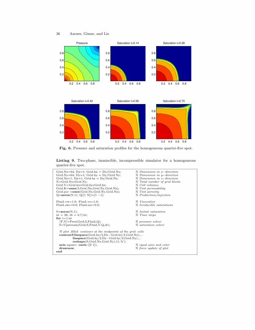
36 Aarnes, Gimse, and Lie
Saturation t=0.14
0.2 0.4 0.6 0.8
0.2
0.4
0.6
0.8
Saturation t=0.28
0.2 0.4 0.6 0.8
0.2
0.4
0.6
0.8
Saturation t=0.42
0.2 0.4 0.6 0.8
0.2
0.4
0.6
0.8
Saturation t=0.56
0.2 0.4 0.6 0.8
0.2
0.4
0.6
0.8
Saturation t=0.70
0.2 0.4 0.6 0.8
0.2
0.4
0.6
0.8
Pressure
0.2 0.4 0.6 0.8
0.2
0.4
0.6
0.8
Fig. 6. Pressure and saturation profiles for the homogeneous quarter-five spot.
Listing 9. Two-phase, immiscible, incompressible simulator for a homogeneousquarter-five spot.
Grid.Nx=64; Dx=1; Grid.hx = Dx/Grid.Nx; % Dimension in x−directionGrid.Ny=64; Dy=1; Grid.hy = Dy/Grid.Ny; % Dimension in y−directionGrid.Nz=1; Dz=1; Grid.hz = Dz/Grid.Nz; % Dimension in z−directionN=Grid.Nx∗Grid.Ny; % Total number of grid blocksGrid.V=Grid.hx∗Grid.hy∗Grid.hz; % Cell volumesGrid.K=ones(3,Grid.Nx,Grid.Ny,Grid.Nz); % Unit permeabilityGrid.por =ones(Grid.Nx,Grid.Ny,Grid.Nz); % Unit porosityQ=zeros(N,1); Q([1 N])=[1 −1]; % Production/injection
Fluid.vw=1.0; Fluid.vo=1.0; % ViscositiesFluid.swc=0.0; Fluid.sor=0.0; % Irreducible saturations
S=zeros(N,1); % Initial saturationnt = 28; dt = 0.7/nt; % Time stepsfor t=1:nt
[P,V]=Pres(Grid,S,Fluid,Q); % pressure solverS=Upstream(Grid,S,Fluid,V,Q,dt); % saturation solver
% plot filled contours at the midpoints of the grid cellscontourf(linspace(Grid.hx/2,Dx−Grid.hx/2,Grid.Nx),...
linspace(Grid.hy/2,Dy−Grid.hy/2,Grid.Ny),...reshape(S,Grid.Nx,Grid.Ny),11,’k’);
axis square; caxis ([0 1]); % equal axes and colordrawnow; % force update of plot
end

An Introduction to the Numerics of Flow in Porous Media using Matlab 37
Listing 9 contains a sequential splitting code for simulating the water in-jection problem up to water-breakthrough in the production well with theexplicit upwind scheme. (For the homogeneous quarter-five spot it is knownthat breakthrough occurs when approximately 0.7 pore-volumes of water havebeen injected). The algorithm is quite simple. First, we set up the grid, thefluid properties and generate the initial saturation distribution. Then, thesolution is advanced in time by repeating the following two steps: (i) solvethe pressure equation and compute edge velocities; (ii) using the fixed edgevelocities, solve the fluid transport equation a time step ∆t.
In Figure 6 we have plotted the initial pressure profile and the saturationprofiles at five equally-spaced time levels as computed on a uniform 64 ×64 grid. The saturation profile consists of a leading shock-wave, in whichwater immediately displaces a fraction of the in situ oil. For a unit viscosityratio, the post-shock saturation value equals
√2/2. Behind the front, the
water saturation is increasing monotonically towards the injector, meaningthat more oil is gradually displaced as more water is injected. Close to theinjector, the level curves are almost circular, corresponding to the circularsymmetry in pressure at the injector. As more water is injected, the leadingwater front develops a finger extending toward and finally breaking throughto the producer.
6.2 An Implicit Solver
Implicit schemes are unconditionally stable in the sense that there is no CFLcondition on the size of the time step. On the other hand, implicit discreti-sation of (43) gives rise to nonlinear systems of equations. Such systems arenormally solved with a Newton or a Newton–Raphson iterative method. Thesemethods typically give second-order convergence, but it is well known thatthey can be very sensitive to the initial guess. It is therefore common to usean alternative technique to compute an initial approximation for each timestep, and then continue with a Newton or Newton–Raphson method.
We shall employ a Newton–Raphson method to solve the implicit system.However, since we do not want to mix too many different methods, we assumethat the initial approximation for each Newton–Raphson iteration (which willbe the saturation field from the previous time step) is sufficiently close to thesolution Sn+1. In practice, this means that one often has to start with smalltime steps after each update of the velocity field. In the code that we presentin Listing 11 the timesteps are selected in a dynamic fashion in order to ensureconvergence. That is, if the Newton–Raphson iteration has not converged inten iterations, then the time step is simply decreased by a factor two so thatthe original timestep is split into two sub-timesteps. If the Newton–Raphsonstill does not converge in less than ten iterations, the original time step is splitinto four sub-timesteps, and so on. In commercial software, the maximumtimestep is controlled by using an estimate of the time discretisation error.Here we have chosen the maximum timestep by convenience to be five days.

38 Aarnes, Gimse, and Lie
Listing 10. Implicit upwind finite-volume discretisation of (43).
function S=NewtRaph(Grid,S,Fluid,V,q,T);
N = Grid.Nx∗Grid.Ny∗Grid.Nz; % number of unknownsA = GenA(Grid,V,q); % system matrix
conv=0; IT=0; S00=S;while conv==0;dt = T/2ˆIT; % timestepdtx = dt./(Grid.V(:)∗Grid.por (:)); % timestep / pore volumefi = max(q,0).∗dtx; % injectionB=spdiags(dtx,0,N,N)∗A;
I=0;while I<2ˆIT; % loop over sub−timestepsS0=S; dsn=1; it=0; I=I+1;
while dsn>1e−3 & it<10; % Newton−Raphson iteration[Mw,Mo,dMw,dMo]=RelPerm(S,Fluid); % mobilities and derivativesdf=dMw./(Mw + Mo)−Mw./(Mw+Mo).ˆ2.∗(dMw+dMo); % df w/dsdG=speye(N)−B∗spdiags(df,0,N,N); % G’(S)
fw = Mw./(Mw+Mo); % fractional flowG = S−S0−(B∗fw+fi); % G(s)ds = −dG\G; % increment dsS = S+ds; % update Sdsn = norm(ds); % norm of incrementit = it+1; % number of N−R iterations
end
if dsn>1e−3; I=2ˆIT; S=S00; end % check for convergenceend
if dsn<1e−3; conv=1; % check for convergenceelse IT=IT+1; end % if not converged, decrease
end % timestep by factor 2
To derive the Newton–Raphson method for the implicit upwind discreti-sation, consider the following homogeneous equation (see (44)):
0 ≡ G(Sn+1) = Sn+1 − Sn − (δtx)T
[Af(Sn+1) +Q+
]. (48)
Assume now that we have obtained an approximation S to the true fix-pointSn+1. Then, by a Taylor expansion, we have
0 = G(Sn+1) ≈ G(S) +G′(S)(Sn+1 − S
),
and a new, and hopefully better, approximation to Sn+1 is obtained by S+dS,where dS satisfies −G′(S)dS = G(S). For the implicit scheme (48) we have
G′(S) = I − (δtx)T Af ′(S),
where f ′(S) = [f ′(si)]i. The code for the fully implicit upwind discretisationis given in Listing 10.
Example 4. In Example 3 we have seen the typical behaviour of a two-phaseoil-water system. Let us now consider a reservoir with a much higher degree

An Introduction to the Numerics of Flow in Porous Media using Matlab 39
Listing 11. Two-phase, immiscible, incompressible simulator for the top layer ofthe SPE-10 model.
Grid.Nx=60; Grid.hx=20∗.3048; % Dimension in x−directionGrid.Ny=220; Grid.hy=10∗.3048; % Dimension in y−directionGrid.Nz=1; Grid.hz=2∗.3048; % Dimension in z−directionN=Grid.Nx∗Grid.Ny∗Grid.Nz; % Number of grid cellesGrid.V=Grid.hx∗Grid.hy∗Grid.hz; % Volume of each cellsFluid.vw=3e−4; Fluid.vo=3e−3; % ViscositiesFluid.swc=0.2; Fluid.sor=0.2; % Irreducible saturationsSt = 5; % Maximum saturation time stepPt = 100; % Pressure time stepND = 2000; % Number of days in simulation
Q=zeros(Grid.Nx,Grid.Ny,1); % Source term for injectionIR=795∗(Grid.Nx∗Grid.Ny/ (60∗220∗85)); % and production. TotalQ(1,1,:)=IR; Q(Grid.Nx,Grid.Ny,:)=−IR; Q=Q(:); % rate scaled to one layer
load Udata; Grid.K=KU(:,1:Grid.Nx,1:Grid.Ny,1); % Permeability in layer 1Por=pU(1:Grid.Nx,1:Grid.Ny,1); % Preprocessed porosity in layer 1Grid.por=max(Por(:),1e−3);
S=Fluid.swc∗ones(N,1); % Initial saturationPc=[0; 1]; Tt=0; % For production curvesfor tp=1:ND/Pt;
[P,V]=Pres(Grid,S,Fluid,Q); % Pressure solverfor ts=1:Pt/St;
S=NewtRaph(Grid,S,Fluid,V,Q,St); % Implicit saturation solversubplot(’position’ ,[0.05 .1 .4 .8]); % Make left subplotpcolor(reshape(S,Grid.Nx,Grid.Ny,Grid.Nz)’); % Plot saturationshading flat; caxis([Fluid.swc 1−Fluid.sor]); %
[Mw,Mo]=RelPerm(S(N),Fluid); Mt=Mw+Mo; % Mobilities in well−blockTt=[Tt,(tp−1)∗Pt+ts∗St]; % Compute simulation timePc=[Pc,[Mw/Mt; Mo/Mt]]; % Append production datasubplot(’position’ ,[0.55 .1 .4 .8]); % Make right subplotplot(Tt,Pc(1,:),Tt,Pc (2,:)); % Plot production dataaxis([0,ND,−0.05,1.05]); % Set correct axislegend(’Water cut’,’Oil cut’ ); % Set legenddrawnow; % Force update of plot
endend
of realism by revisiting the two-dimensional SPE-10 models from Example 2.We consider an incompressible oil-water system, for which swc = sor = 0.2,µw = 0.3 cp, and µo = 3.0 cp. The reservoir is initially filled with oil, meaningthat the initial water saturation is equal the connate water saturation s(x, 0) ≡swc. The porosity is strongly correlated with the horizontal permeability andcontains about 2.5% zero values. To avoid division by zero in these cells, wesimply replace the zero values by a certain minimal nonzero value.
Listing 11 contains a simulation routine that loads data and computes theflow using sequential splitting. Since both the porosity and permeability hasa strongly heterogeneous structure spanning several orders of magnitude it isnot practical to use the explicit scheme due to the inordinately large numberof time steps enforced by the stability condition. Instead we use an implicitscheme—the Newton–Raphson method presented in Listing 10.

40 Aarnes, Gimse, and Lie
10 20 30 40 50 60
20
40
60
80
100
120
140
160
180
200
220
0 500 1000 1500 2000
0
0.1
0.2
0.3
0.4
0.5
0.6
0.7
0.8
0.9
1 Water cut
Oil cut
10 20 30 40 50 60
20
40
60
80
100
120
140
160
180
200
220
0 500 1000 1500 2000
0
0.1
0.2
0.3
0.4
0.5
0.6
0.7
0.8
0.9
1 Water cut
Oil cut
10 20 30 40 50 60
20
40
60
80
100
120
140
160
180
200
220
0 500 1000 1500 2000
0
0.1
0.2
0.3
0.4
0.5
0.6
0.7
0.8
0.9
1 Water cut
Oil cut
10 20 30 40 50 60
20
40
60
80
100
120
140
160
180
200
220
0 500 1000 1500 2000
0
0.1
0.2
0.3
0.4
0.5
0.6
0.7
0.8
0.9
1 Water cut
Oil cut
Fig. 7. Saturation and production profiles after 400, 800, 1200, and 2000 days ofproduction for the Tarbert formation in the top layer of the SPE-10 model.
10 20 30 40 50 60
20
40
60
80
100
120
140
160
180
200
220
0 500 1000 1500 2000
0
0.1
0.2
0.3
0.4
0.5
0.6
0.7
0.8
0.9
1 Water cut
Oil cut
10 20 30 40 50 60
20
40
60
80
100
120
140
160
180
200
220
0 500 1000 1500 2000
0
0.1
0.2
0.3
0.4
0.5
0.6
0.7
0.8
0.9
1 Water cut
Oil cut
10 20 30 40 50 60
20
40
60
80
100
120
140
160
180
200
220
0 500 1000 1500 2000
0
0.1
0.2
0.3
0.4
0.5
0.6
0.7
0.8
0.9
1 Water cut
Oil cut
10 20 30 40 50 60
20
40
60
80
100
120
140
160
180
200
220
0 500 1000 1500 2000
0
0.1
0.2
0.3
0.4
0.5
0.6
0.7
0.8
0.9
1 Water cut
Oil cut
Fig. 8. Saturation and production profiles after 400, 800, 1200, and 2000 days ofproduction for the Upper Ness formation in the bottom layer of the SPE-10 model.

An Introduction to the Numerics of Flow in Porous Media using Matlab 41
Figures 7 and 8 show saturation and production profiles during the simu-lation for the top and bottom layers in the SPE-10 model. In the figures, oiland water cuts refer to the fractional flows of oil and water, respectively, intothe production well. Here we clearly see that the spaghetti of channelling sys-tems that we have in the Upper Ness formation leads to a very different flowscenario from what we observed in the top layer, which has a quite smoothpermeability distribution compared to the bottom layer.
References
1. J.E. Aarnes, K.-A. Lie, and A.B. Rustad. Modelling of multiscale structures inflow simulations for petroleum reservoirs. In G. Hasle, K.-A. Lie, and E. Quak,editors, Geometrical Modeling, Numerical Simulation and Optimization: Indus-trial Mathematics at SINTEF. Springer Verlag.
2. I. Aavatsmark, T. Barkve, Ø. Bøe, and T. Mannseth. Discretization on un-structured grids for inhomogeneous, anisotropic media. part i: Derivation of themethods. Siam J. Sci. Comp., 19(5):1700–1716, 1998.
3. I. Aavatsmark, T. Barkve, Ø. Bøe, and T. Mannseth. Discretization on un-structured grids for inhomogeneous, anisotropic media. part ii: Discussion andnumerical results. Siam J. Sci. Comp., 19(5):1717–1736, 1998.
4. T. Arbogast. An overview of subgrid upscaling for elliptic problems in mixedform. In Z. Chen, R. Glowinski, and K. Li, editors, Current trends in scientificcomputing, Contemporary Mathematics, pages 21–32. AMS, 2003.
5. T. Arbogast. Analysis of a two-scale, locally conservative subgrid upscaling forelliptic problems. SIAM J. Numer. Anal., 42(2):576–598, 2004.
6. K. Aziz and A. Settari. Petroleum reservoir simulation. Elsevier, London andNew York, 1979.
7. J.W. Barker and S. Thibeau. A critical review of the use of pseudorelativepermeabilities for upscaling. SPE Reservoir Eng., 12:138–143, 1997.
8. D. Braess. Finite elements: Theory fast solvers and applications in solid me-chanics. Cambridge University Press, Cambridge, 1997.
9. S.C. Brenner and L.R. Scott. The mathematical theory of finite element methods.Springer–Verlag, New York, 1994.
10. F. Brezzi and M. Fortin. Mixed and hybrid finite element methods. Computa-tional Mathematics. Springer–Verlag, New York, 1991.
11. G. Chavent and J. Jaffre. Mathematical models and finite elements for reservoirsimulation. North Holland, 1982.
12. Z. Chen and T.Y. Hou. A mixed multiscale finite element method for ellipticproblems with oscillating coefficients. Math. Comp., 72:541–576, 2003.
13. M. A. Christie and M. J. Blunt. Tenth SPE comparative solution project: Acomparison of upsc aling techniques. SPE, 72469, 2001. url: www.spe.org/csp.
14. M.A. Christie. Upscaling for reservoir simulation. JPT J. Pet. Tech., 48:1004–1010, 1996.
15. L.P. Dake. Fundamentals of reservoir engineering. Elsevier, Amsterdam, 1978.16. M. Delshad and G.A Pope. Comparison of the three-phase relative permeability
models. Transp. Porous Media, 4:59–83, 1979.17. A.H. Demond and P.V. Roberts. An examination of relative permeability rela-
tions for two-phase flow in porous media. Water Res. Bull., 23:617–628, 1987.

42 Aarnes, Gimse, and Lie
18. Bjorn Engquist and Weinan E. The heterogeneous multi-scale methods. Comm.Math. Sci., 1:87–133, 2003.
19. Bjorn Engquist and Weinan E. Multiscale modeling and computation. Noticesof the AMS, 50(9):1062–1070, 2003.
20. R.E. Ewing. The mathematics of reservoir simulation. SIAM, 1983.21. T.R. Hagen, M.O. Henriksen, J.M. Hjelmervik, and K.-A. Lie. How to solve
systems of conservation laws numerically using the graphics processor as a high-performance computational engine. In G. Hasle, K.-A. Lie, and E. Quak, edi-tors, Geometrical Modeling, Numerical Simulation and Optimization: IndustrialMathematics at SINTEF. Springer Verlag.
22. H.H. Haldorsen and C.J. MacDonald. Stochastic modeling of underground reser-voir facies. SPE Preprint, 16751:99–113, 1987.
23. M. Honarpour and S.M. Mahmood. Relative-permeability measurements: Anoverview. J.Petr. Tech, 40:963–966, 1988.
24. T.Y. Hou and X-H. Wu. A multiscale finite element method for elliptic problemsin composite materials and porous media. J. Comput. Phys., 134:169–189, 1997.
25. R. Juanes and T.W. Patzek. Relative permeabilities for strictly hyperbolicmodels of three-phase flow in porous media. Tranp. Porous Media, 57(2):125–152, 2004.
26. R. Juanes and T.W. Patzek. Three-phase displacement theory: an improveddescription of relative permeabilities. SPE Journal, September 2004.
27. L. Lake. Enhanced oil recovery. Prentice Hall, Inglewood Cliffs, NJ, 1989.28. B.B. Maini and T. Okazawa. Effects of temperature on heavy oil-water relative
permeability. J. Can. Petr. Tech, 26:33–41, 1987.29. D.W. Peaceman. Fundamentals of numerical reservoir simulation. Elsevier,
Amsterdam, 1977.30. P.A. Raviart and J.M. Thomas. A mixed finite element method for second order
elliptic equations. In I. Galligani and E. Magenes, editors, Mathematical Aspectsof Finite Element Methods, pages 292–315. Springer–Verlag, Berlin – Heidelberg– New York, 1977.
31. P. Renard and G. de Marsily. Calculating equivalent permeability. Adv. WaterRes., 20:253–278, 1997.
32. H.L. Stone. Estimation of three-phase relative permeability and residual oil. J.Can. Petr. Tech, 12:53–61, 1973.
33. S.M. Skjæveland and Jon Kleppe, editors. SPOR Monograph, Recent advancesin improved oil recovery methods for north sea sandstone reservoirs. NorwegianPetroleum Directorate, Norway, 1992.