Flow in Porous Media

Module 4.a Diffusive and Convective Flow

Shahab Gerami

Outline

Convection

Diffusion

Convection and Diffusion

Diffusion coefficient in porous media

Modeling 1-D Diffusion Equation

Diffusivity Coefficient of Gases in Bitumen- Inverse solution approach

Convection

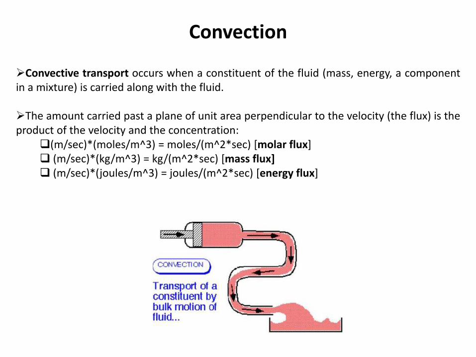
Convective transport occurs when a constituent of the fluid (mass, energy, a component in a mixture) is carried along with the fluid.

The amount carried past a plane of unit area perpendicular to the velocity (the flux) is the product of the velocity and the concentration:

(m/sec)*(moles/m^3) = moles/(m^2*sec) [molar flux] (m/sec)*(kg/m^3) = kg/(m^2*sec) [mass flux] (m/sec)*(joules/m^3) = joules/(m^2*sec) [energy flux]

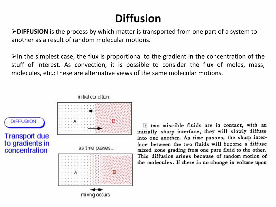
Diffusion DIFFUSION is the process by which matter is transported from one part of a system to another as a result of random molecular motions.

In the simplest case, the flux is proportional to the gradient in the concentration of the stuff of interest. As convection, it is possible to consider the flux of moles, mass, molecules, etc.: these are alternative views of the same molecular motions.

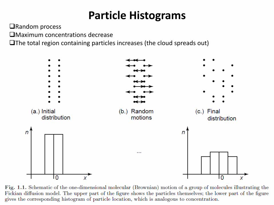
Particle Histograms Random process Maximum concentrations decrease The total region containing particles increases (the cloud spreads out)

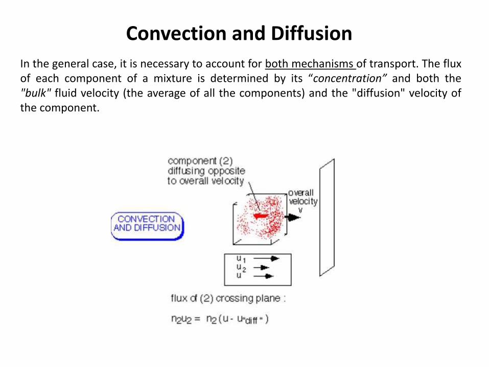
Convection and Diffusion

In the general case, it is necessary to account for both mechanisms of transport. The flux of each component of a mixture is determined by its “concentration” and both the "bulk" fluid velocity (the average of all the components) and the "diffusion" velocity of the component.

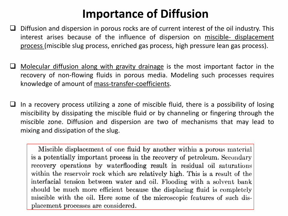
Importance of Diffusion Diffusion and dispersion in porous rocks are of current interest of the oil industry. This

interest arises because of the influence of dispersion on miscible- displacement process (miscible slug process, enriched gas process, high pressure lean gas process).

Molecular diffusion along with gravity drainage is the most important factor in the recovery of non-flowing fluids in porous media. Modeling such processes requires knowledge of amount of mass-transfer-coefficients.

In a recovery process utilizing a zone of miscible fluid, there is a possibility of losing miscibility by dissipating the miscible fluid or by channeling or fingering through the miscible zone. Diffusion and dispersion are two of mechanisms that may lead to mixing and dissipation of the slug.

Diffusion is the resulting net transport of molecules from a region of higher concentration to one of lower concentration.

Diffusion coefficient D is a measurement which gives the speed at which the molecules of component A can penetrate component B when they come into contact with each other under given external and/or internal conditions.

Generally, D= f(ΔC, T, P, IFT); however, it is often possible to represent diffusive behavior approximately by selecting an average diffusivity coefficient.

Diffusion coefficient D

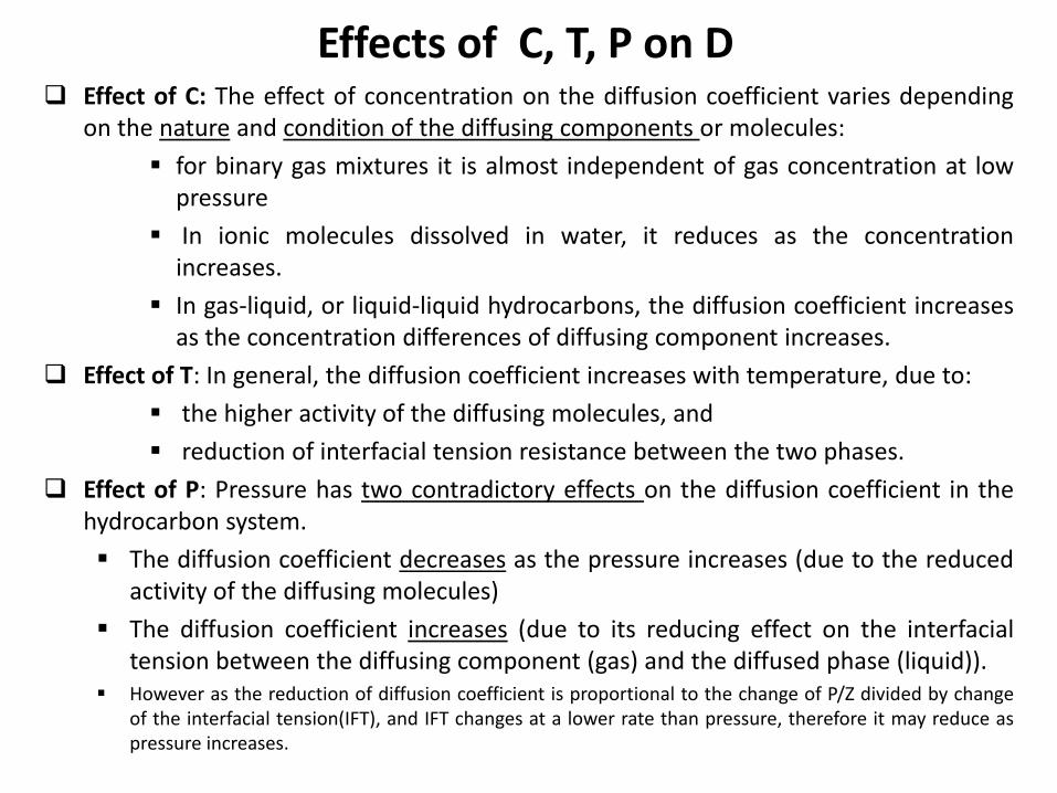
Effects of C, T, P on D Effect of C: The effect of concentration on the diffusion coefficient varies depending

on the nature and condition of the diffusing components or molecules:

for binary gas mixtures it is almost independent of gas concentration at low pressure

In ionic molecules dissolved in water, it reduces as the concentration increases.

In gas-liquid, or liquid-liquid hydrocarbons, the diffusion coefficient increases as the concentration differences of diffusing component increases.

Effect of T: In general, the diffusion coefficient increases with temperature, due to:

the higher activity of the diffusing molecules, and

reduction of interfacial tension resistance between the two phases.

Effect of P: Pressure has two contradictory effects on the diffusion coefficient in the hydrocarbon system.

The diffusion coefficient decreases as the pressure increases (due to the reduced activity of the diffusing molecules)

The diffusion coefficient increases (due to its reducing effect on the interfacial tension between the diffusing component (gas) and the diffused phase (liquid)).

However as the reduction of diffusion coefficient is proportional to the change of P/Z divided by change of the interfacial tension(IFT), and IFT changes at a lower rate than pressure, therefore it may reduce as pressure increases.

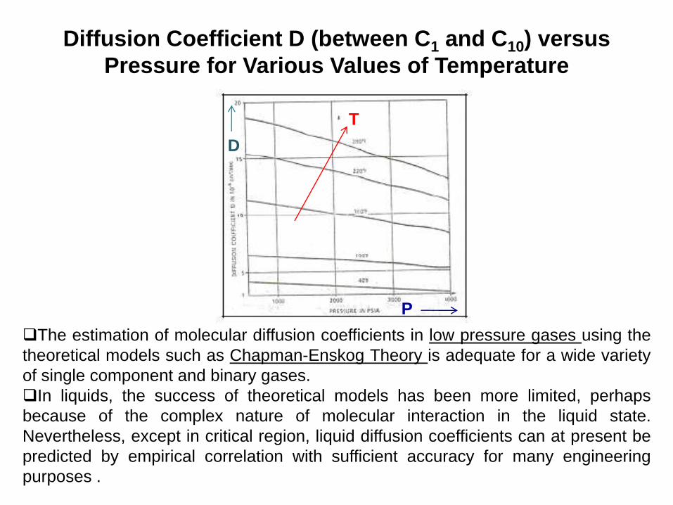
Diffusion Coefficient D (between C1 and C10) versus

Pressure for Various Values of Temperature

The estimation of molecular diffusion coefficients in low pressure gases using the

theoretical models such as Chapman-Enskog Theory is adequate for a wide variety

of single component and binary gases.

In liquids, the success of theoretical models has been more limited, perhaps

because of the complex nature of molecular interaction in the liquid state.

Nevertheless, except in critical region, liquid diffusion coefficients can at present be

predicted by empirical correlation with sufficient accuracy for many engineering

purposes .

D

P

T

Diffusion Coefficient for Binary Gas Systems at low Pressures:

Fuller et al correlation

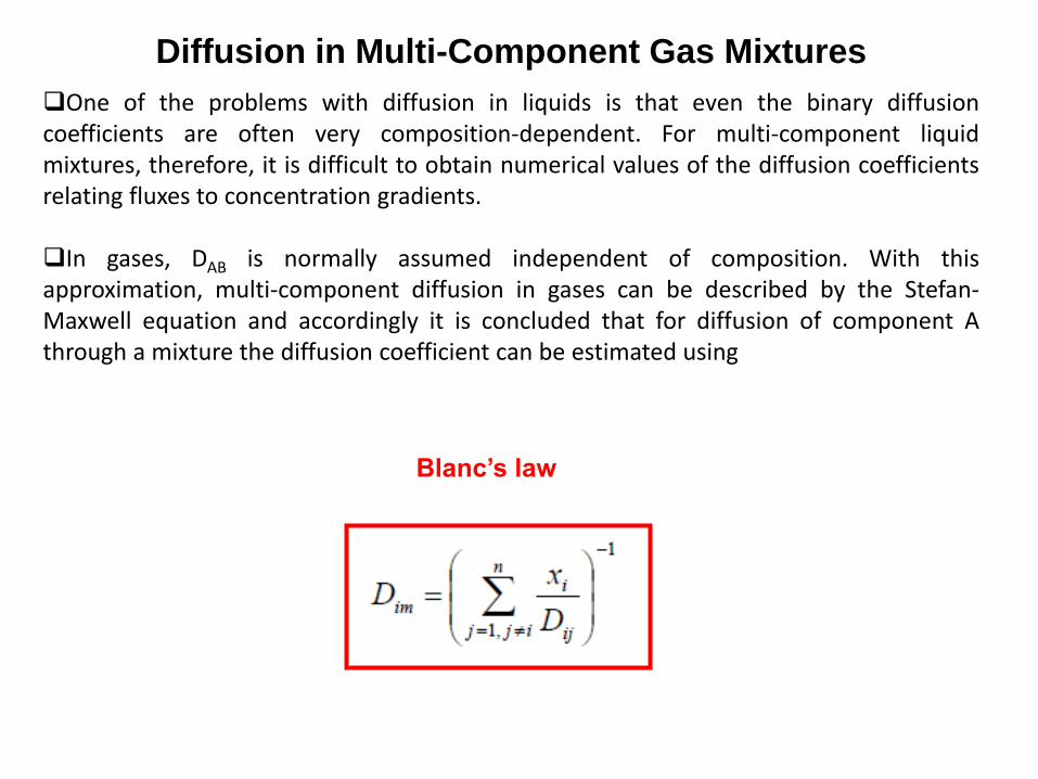
Diffusion in Multi-Component Gas Mixtures

One of the problems with diffusion in liquids is that even the binary diffusion coefficients are often very composition-dependent. For multi-component liquid mixtures, therefore, it is difficult to obtain numerical values of the diffusion coefficients relating fluxes to concentration gradients.

In gases, DAB is normally assumed independent of composition. With this approximation, multi-component diffusion in gases can be described by the Stefan- Maxwell equation and accordingly it is concluded that for diffusion of component A through a mixture the diffusion coefficient can be estimated using

Blanc’s law

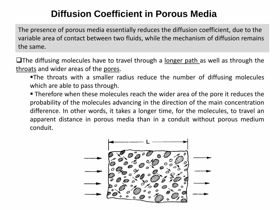
Diffusion Coefficient in Porous Media

The presence of porous media essentially reduces the diffusion coefficient, due to the variable area of contact between two fluids, while the mechanism of diffusion remains the same.

The diffusing molecules have to travel through a longer path as well as through the throats and wider areas of the pores.

The throats with a smaller radius reduce the number of diffusing molecules which are able to pass through. Therefore when these molecules reach the wider area of the pore it reduces the probability of the molecules advancing in the direction of the main concentration difference. In other words, it takes a longer time, for the molecules, to travel an apparent distance in porous media than in a conduit without porous medium conduit.

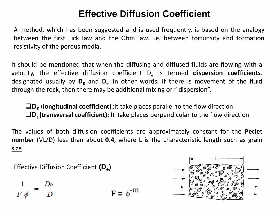
Effective Diffusion Coefficient

A method, which has been suggested and is used frequently, is based on the analogy between the first Fick law and the Ohm law, i.e. between tortuosity and formation resistivity of the porous media.

It should be mentioned that when the diffusing and diffused fluids are flowing with a velocity, the effective diffusion coefficient De is termed dispersion coefficients, designated usually by Dℓ and Dt. In other words, If there is movement of the fluid through the rock, then there may be additional mixing or “ dispersion”.

Dℓ (longitudinal coefficient) :It take places parallel to the flow direction Dt (transversal coefficient): It take places perpendicular to the flow direction

The values of both diffusion coefficients are approximately constant for the Peclet number (VL/D) less than about 0.4, where L is the characteristic length such as grain size.

Effective Diffusion Coefficient (De)

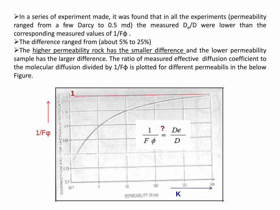
In a series of experiment made, it was found that in all the experiments (permeability ranged from a few Darcy to 0.5 md) the measured De/D were lower than the corresponding measured values of 1/Fφ . The difference ranged from (about 5% to 25%) The higher permeability rock has the smaller difference and the lower permeability sample has the larger difference. The ratio of measured effective diffusion coefficient to the molecular diffusion divided by 1/Fφ is plotted for different permeabilis in the below Figure.

K

1/Fφ

1

?

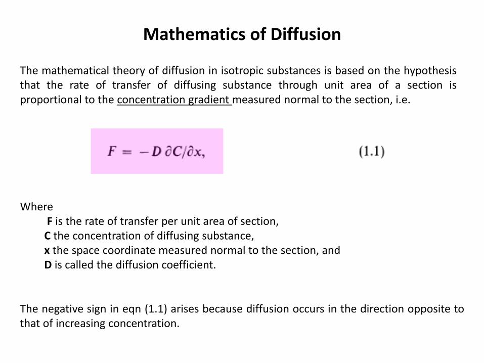
Mathematics of Diffusion

The mathematical theory of diffusion in isotropic substances is based on the hypothesis that the rate of transfer of diffusing substance through unit area of a section is proportional to the concentration gradient measured normal to the section, i.e.

Where F is the rate of transfer per unit area of section, C the concentration of diffusing substance, x the space coordinate measured normal to the section, and D is called the diffusion coefficient.

The negative sign in eqn (1.1) arises because diffusion occurs in the direction opposite to that of increasing concentration.

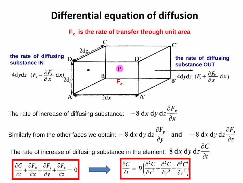
Differential equation of diffusion

the rate of diffusing

substance IN the rate of diffusing

substance OUT

Fx is the rate of transfer through unit area

Fx

The rate of increase of diffusing substance:

Similarly from the other faces we obtain:

The rate of increase of diffusing substance in the element:

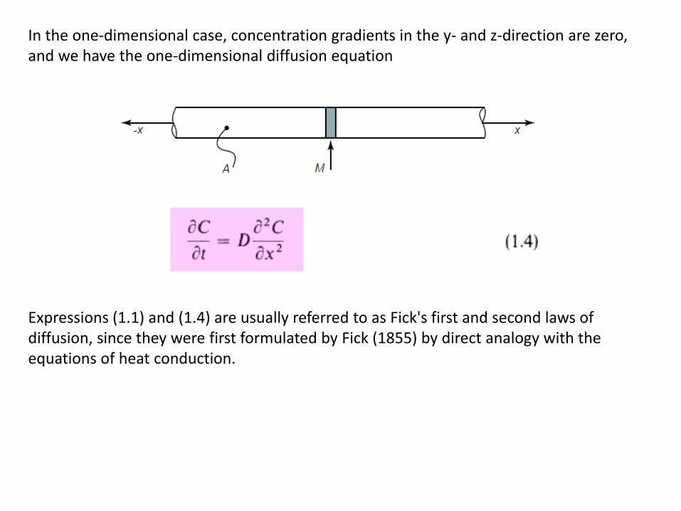
In the one-dimensional case, concentration gradients in the y- and z-direction are zero, and we have the one-dimensional diffusion equation

Expressions (1.1) and (1.4) are usually referred to as Fick's first and second laws of diffusion, since they were first formulated by Fick (1855) by direct analogy with the equations of heat conduction.

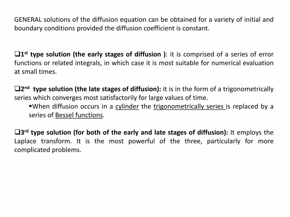
GENERAL solutions of the diffusion equation can be obtained for a variety of initial and boundary conditions provided the diffusion coefficient is constant. 1st type solution (the early stages of diffusion ): it is comprised of a series of error functions or related integrals, in which case it is most suitable for numerical evaluation at small times.

2nd type solution (the late stages of diffusion): it is in the form of a trigonometrically series which converges most satisfactorily for large values of time.

When diffusion occurs in a cylinder the trigonometrically series is replaced by a series of Bessel functions.

3rd type solution (for both of the early and late stages of diffusion): It employs the Laplace transform. It is the most powerful of the three, particularly for more complicated problems.

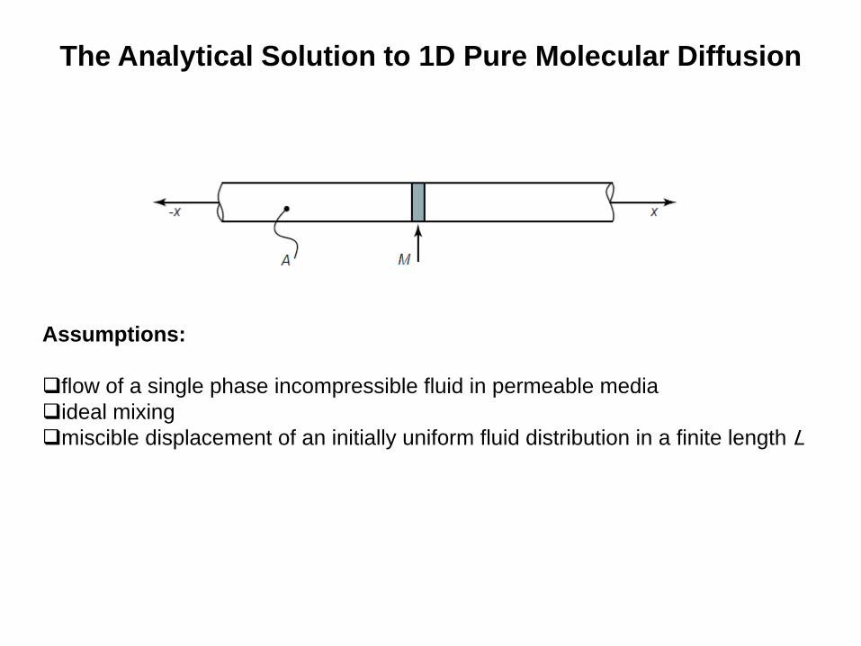
The Analytical Solution to 1D Pure Molecular Diffusion

Assumptions:

flow of a single phase incompressible fluid in permeable media

ideal mixing

miscible displacement of an initially uniform fluid distribution in a finite length L

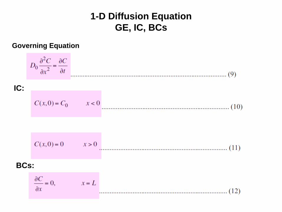
1-D Diffusion Equation

GE, IC, BCs

IC:

BCs:

Governing Equation

1-D Diffusion Equation

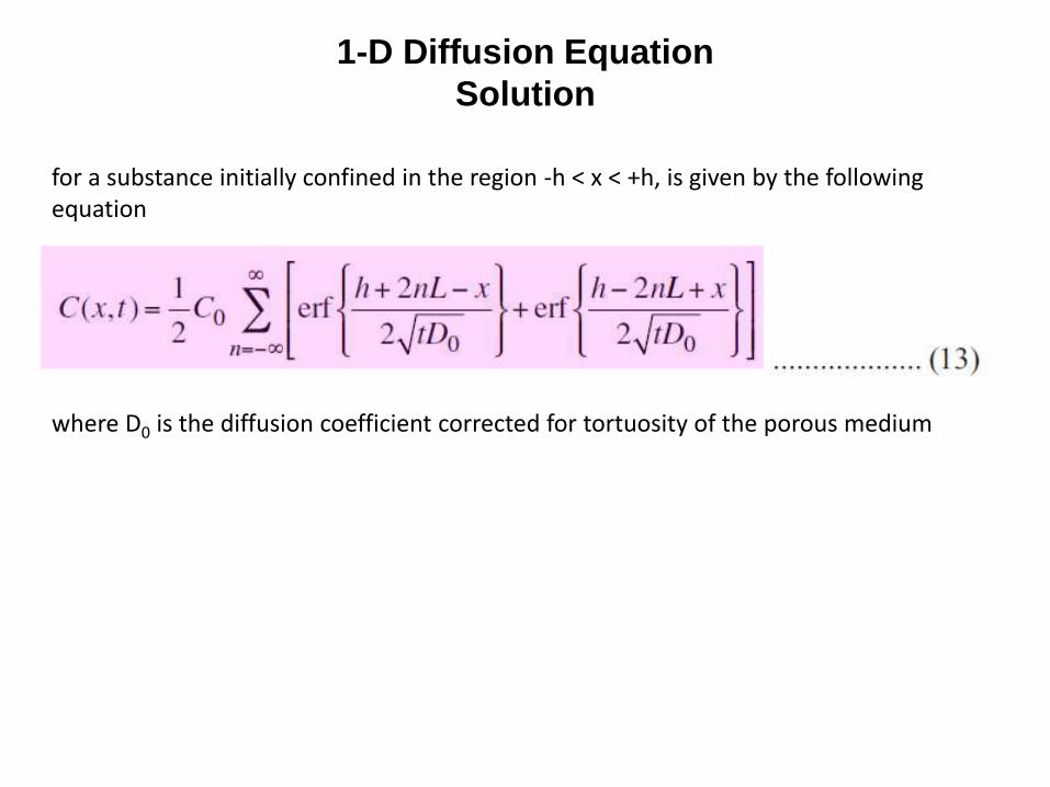
Solution

for a substance initially confined in the region -h < x < +h, is given by the following equation

where D0 is the diffusion coefficient corrected for tortuosity of the porous medium

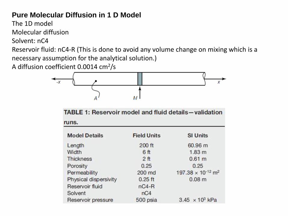
Pure Molecular Diffusion in 1 D Model The 1D model Molecular diffusion Solvent: nC4 Reservoir fluid: nC4-R (This is done to avoid any volume change on mixing which is a necessary assumption for the analytical solution.) A diffusion coefficient 0.0014 cm2/s

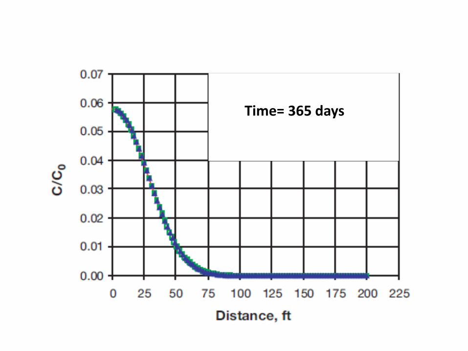
Time= 365 days

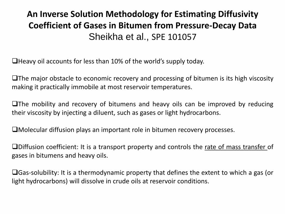
Heavy oil accounts for less than 10% of the world’s supply today.

The major obstacle to economic recovery and processing of bitumen is its high viscosity making it practically immobile at most reservoir temperatures.

The mobility and recovery of bitumens and heavy oils can be improved by reducing their viscosity by injecting a diluent, such as gases or light hydrocarbons.

Molecular diffusion plays an important role in bitumen recovery processes.

Diffusion coefficient: It is a transport property and controls the rate of mass transfer of gases in bitumens and heavy oils.

Gas-solubility: It is a thermodynamic property that defines the extent to which a gas (or light hydrocarbons) will dissolve in crude oils at reservoir conditions.

An Inverse Solution Methodology for Estimating Diffusivity Coefficient of Gases in Bitumen from Pressure-Decay Data

Sheikha et al., SPE 101057

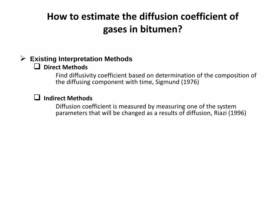
Existing Interpretation Methods

Direct Methods Find diffusivity coefficient based on determination of the composition of

the diffusing component with time, Sigmund (1976)

Indirect Methods Diffusion coefficient is measured by measuring one of the system

parameters that will be changed as a results of diffusion, Riazi (1996)

How to estimate the diffusion coefficient of gases in bitumen?

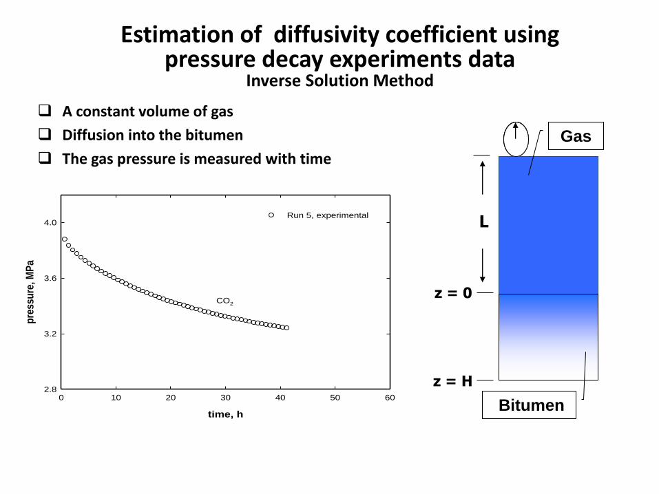
Estimation of diffusivity coefficient using pressure decay experiments data

Inverse Solution Method

A constant volume of gas

Diffusion into the bitumen

The gas pressure is measured with time

L

z = 0

Gas

Bitumen

z = H

time, h

0 10 20 30 40 50 60

pre

ss

ure

, MP

a

2.8

3.2

3.6

4.0Run 5, experimental

CO2

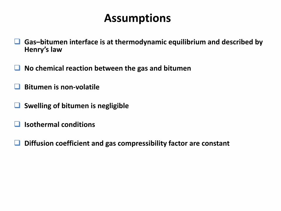
Assumptions

Gas–bitumen interface is at thermodynamic equilibrium and described by Henry’s law

No chemical reaction between the gas and bitumen

Bitumen is non-volatile

Swelling of bitumen is negligible

Isothermal conditions

Diffusion coefficient and gas compressibility factor are constant

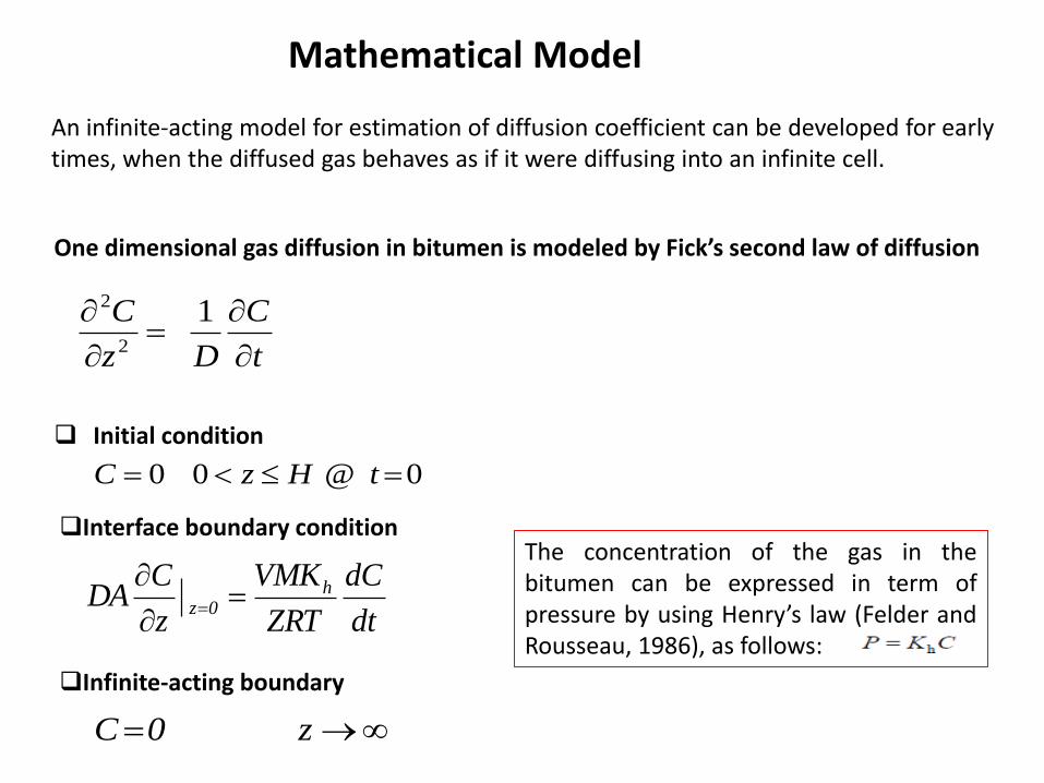
Mathematical Model

An infinite-acting model for estimation of diffusion coefficient can be developed for early times, when the diffused gas behaves as if it were diffusing into an infinite cell.

One dimensional gas diffusion in bitumen is modeled by Fick’s second law of diffusion

Initial condition

t

C

Dz

C

12

2

0@00 tHzC

Interface boundary condition

dt

dC

ZRT

VMK

z

CDA h

0z

The concentration of the gas in the bitumen can be expressed in term of pressure by using Henry’s law (Felder and Rousseau, 1986), as follows:

Infinite-acting boundary

z0C

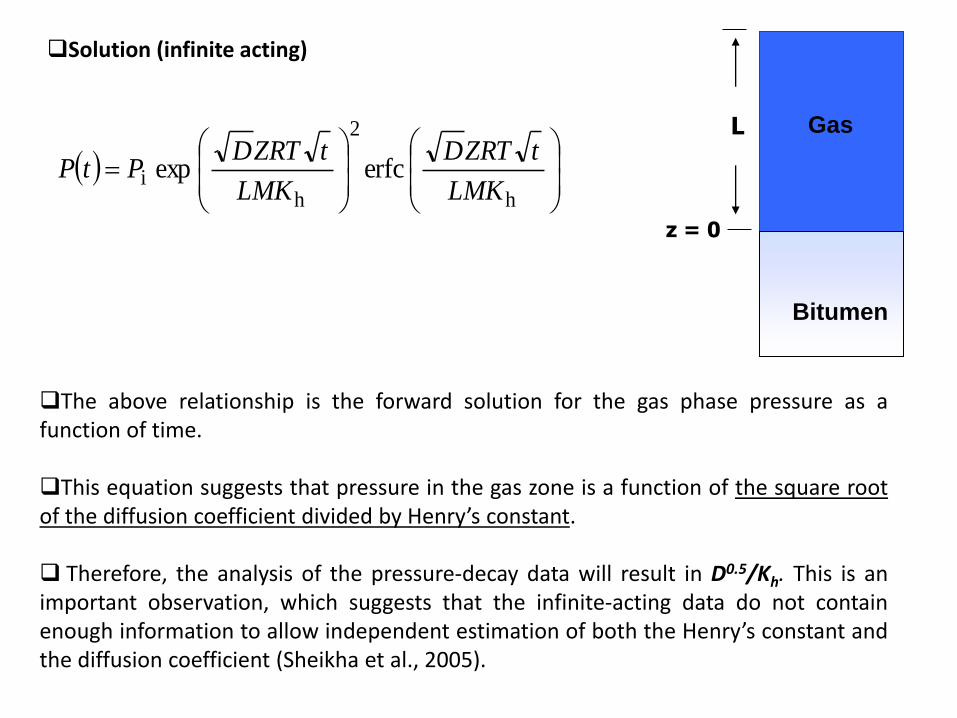
Solution (infinite acting)

h

2

hi erfc exp

LMK

tZRTD

LMK

tZRTDPtP

The above relationship is the forward solution for the gas phase pressure as a function of time.

This equation suggests that pressure in the gas zone is a function of the square root of the diffusion coefficient divided by Henry’s constant.

Therefore, the analysis of the pressure-decay data will result in D0.5/Kh. This is an important observation, which suggests that the infinite-acting data do not contain enough information to allow independent estimation of both the Henry’s constant and the diffusion coefficient (Sheikha et al., 2005).

L

z = 0

Bitumen

Gas

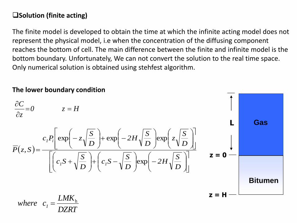
The finite model is developed to obtain the time at which the infinite acting model does not represent the physical model, i.e when the concentration of the diffusing component reaches the bottom of cell. The main difference between the finite and infinite model is the bottom boundary. Unfortunately, We can not convert the solution to the real time space. Only numerical solution is obtained using stehfest algorithm.

Solution (finite acting)

L

z = 0

z = H

Bitumen

Gas

The lower boundary condition

D

SH2

D

SSc

D

SSc

D

Sz

D

SH2

D

SzPc

SzP

11

i1

exp

expexpexp

,

Hz0z

C

DZRT

LMKcwhere 1

h

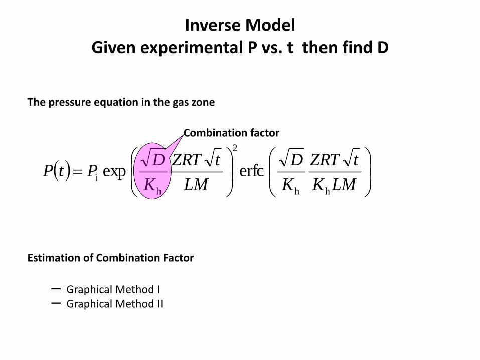
Inverse Model Given experimental P vs. t then find D

The pressure equation in the gas zone

Estimation of Combination Factor

– Graphical Method I – Graphical Method II

LMK

tZRT

K

D

LM

tZRT

K

DPtP

hh

2

h

i erfc exp

Combination factor

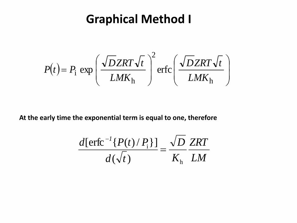
Graphical Method I

At the early time the exponential term is equal to one, therefore

h

2

hi erfc exp

LMK

tZRTD

LMK

tZRTDPtP

LM

ZRT

K

D

td

PtPd 1

h

i

)(

}]/)({erfc[

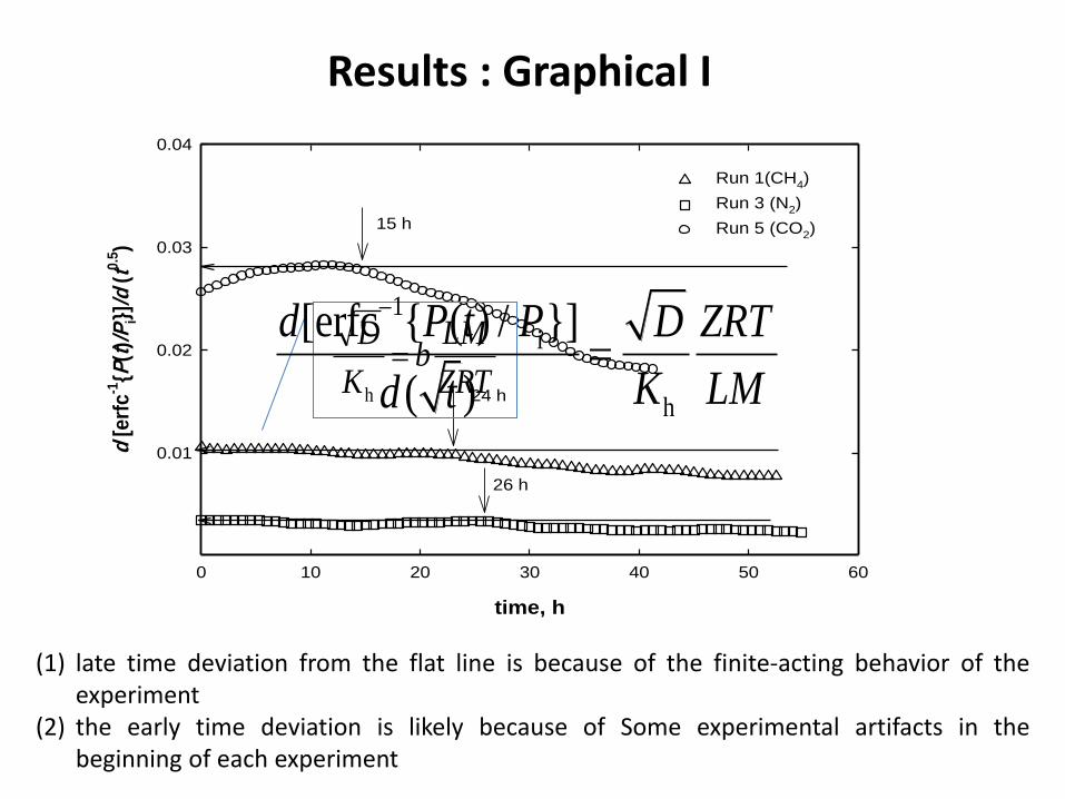
Results : Graphical I

time, h

0 10 20 30 40 50 60

d [

erf

c-1

{P(t

)/P

i}]/

d (

t0.5

)

0.01

0.02

0.03

0.04

Run 1(CH4)

Run 3 (N2)

Run 5 (CO2)15 h

24 h

26 h

ZRT

LMb

K

D

hb

1

i

h

[erfc { ( ) / }]

( )

d P t P D ZRT

K LMd t

T=75 C

(1) late time deviation from the flat line is because of the finite-acting behavior of the experiment

(2) the early time deviation is likely because of Some experimental artifacts in the beginning of each experiment

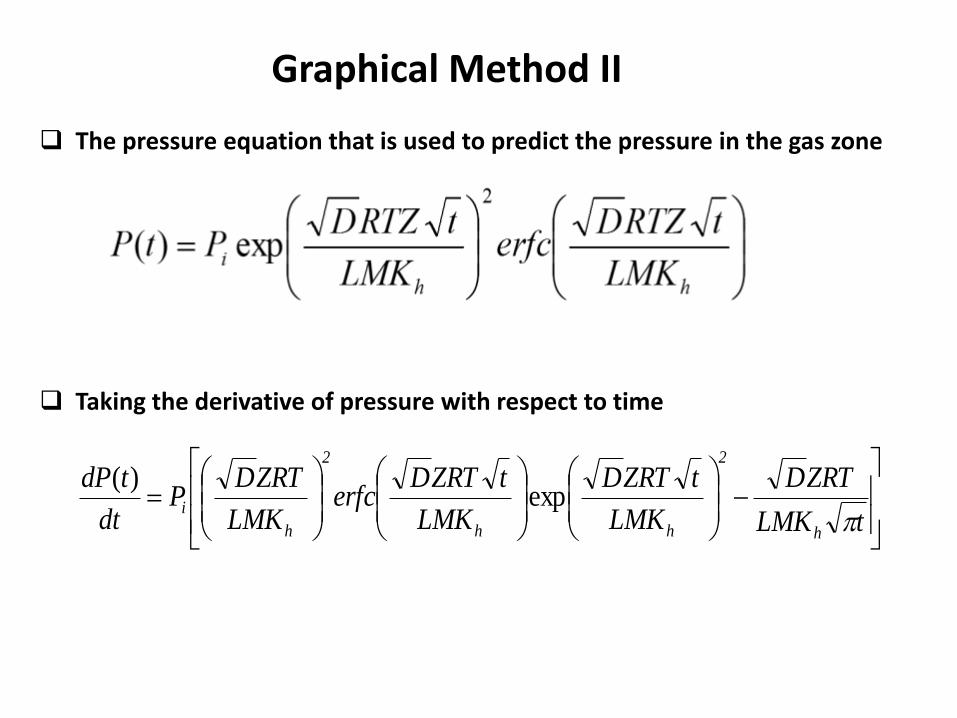
Graphical Method II

The pressure equation that is used to predict the pressure in the gas zone

Taking the derivative of pressure with respect to time

tLMK

ZRTD

LMK

tZRTD

LMK

tZRTDerfc

LMK

ZRTDP

dt

tdP

h

2

hh

2

h

i

exp)(

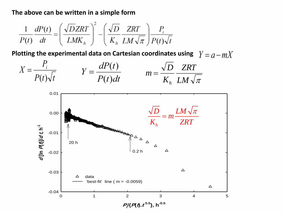
The above can be written in a simple form

Plotting the experimental data on Cartesian coordinates using

LM

ZRT

K

Dm

h

Pi/{P(t).t 0.5

}, h-0.5

0 1 2 3 4 5

d [

ln P

(t)]

/d t

, h-1

-0.04

-0.03

-0.02

-0.01

0.00

0.01

data

'best-fit' line ( m = -0.0059)

0.2 h

20 h

h

D LMm

K ZRT

7/1/2013 37

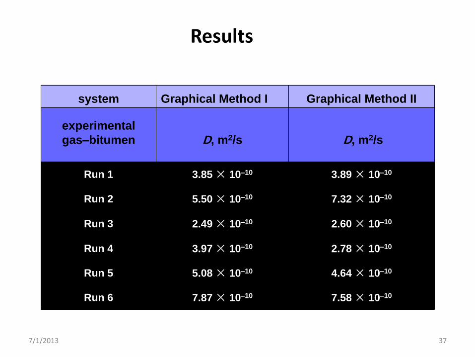
Results

system Graphical Method I Graphical Method II

experimental

gas–bitumen

D, m2/s

D, m2/s

Run 1 3.85 × 10–10 3.89 × 10–10

Run 2 5.50 × 10–10 7.32 × 10–10

Run 3 2.49 × 10–10 2.60 × 10–10

Run 4 3.97 × 10–10 2.78 × 10–10

Run 5 5.08 × 10–10 4.64 × 10–10

Run 6 7.87 × 10–10 7.58 × 10–10