an admittance shaping controller for exoskeleton ... · chronizing exoskeleton torques to the...
TRANSCRIPT

Autonomous Robots manuscript No.(will be inserted by the editor)
An admittance shaping controller for exoskeleton assistance of the lowerextremities
Gabriel Aguirre-Ollinger · Umashankar Nagarajan · Ambarish Goswami ·
Received: date / Accepted: date
Abstract We present a method for lower-limb exoskeletoncontrol that defines assistance as a desired dynamic responsefor the human leg. Wearing the exoskeleton can be seen asreplacing the leg’s natural admittance with the equivalentad-mittance of the coupled system. The control goal is to makethe leg obey an admittance model defined by target valuesof natural frequency, peak magnitude and zero-frequency re-sponse. No estimation of muscle torques or motion intent isnecessary. Instead, the controller scales up the coupled sys-tem’s sensitivity transfer function by means of a compen-sator employing positive feedback. This approach increasesthe leg’s mobility and makes the exoskeleton an active de-vice capable of performing net positive work on the limb.Although positive feedback is usually considered destabiliz-ing, here performance and robust stability are successfullyachieved through a constrained optimization that maximizesthe system’s gain margins while ensuring the desired loca-tion of its dominant poles.
Keywords Exoskeleton· Assistive robotics· Interactioncontrol· Admittance control
Notation
Our control method is formulated in terms of Laplace-domaintransfer functions. Here we explain the notation employed:
• Transfer functions.
This research was supported by a grant from the Honda Research In-stitute, Mountain View, CA, USA.
G. Aguirre-OllingerCentre for Autonomous Systems, University of Technology, Sydney,Broadway 2007, AustraliaE-mail: [email protected]
U. Nagarajan· A. GoswamiHonda Research Institute, Mountain View, CA 94043, USA
• Z (s): mechanical impedance.• Y (s): mechanical admittance.• X (s): integral of the mechanical admittance (X (s) =
Y (s)/s).• S (s): sensitivity transfer function. This is a closed-
loop transfer function that evaluates to 1 at all fre-quencies when the feedback gain is zero.
• T (s): complementary sensitivity transfer function,given byT (s) = 1− S (s).
• L (s): loop transfer function for root-locus analysis.• N (s): numerator of a rational transfer function.• D (s): denominator of a rational transfer function.• W (s): loop transfer function for robustness analysis
(sec. 4).• Subscriptsare used to indicate which subsystems are
present in a particular transfer function.• h: human leg.• e: exoskeleton mechanism, consisting of the actuator
and arm.• c: compliant coupling between the human leg and
the exoskeleton mechanism, modeled as a spring anddamper.
• f : feedback compensator for the exoskeleton.
1 Introduction
Exoskeletons are wearable mechanical devices that possessa kinematic configuration similar to that of the human bodyand have the ability to follow the movements of the user’sextremities. Powered exoskeletons are usually designed toproduce contact forces to assist the user in performing a mo-tor task. In recent years, a large number of lower-limb exo-skeleton systems and their associated control methods havebeen developed, either as research tools for the study of hu-man gait (Ferris et al, 2007; Emken et al, 2006), or as reha-

2 Gabriel Aguirre-Ollinger et al.
bilitation tools for patients with stroke and other locomotordisorders (Dollar and Herr, 2008b). In a parallel develop-ment, a number of lightweight, autonomous exoskeletonshave been designed with the aim of assisting impaired oraged users in daily-living situations (Ekso BionicsTM, 2013;American Honda Motor Co., Inc., 2009). This research aimsto develop a general-purpose exoskeleton control that min-imizes the need for estimating the user’s intended motion.Our primary target application is autonomous exoskeletonsfor daily living.
1.1 A classification of exoskeleton-based assistivestrategies
Together with the physical exoskeletons, a wide variety ofassistive strategies have been developed and tested with vary-ing levels of success. Below we present a compact classifi-cation of strategies for aiding human locomotion, along witha few examples that are currently available in the literature.
1. Based on what aspect of the body’s movement is sup-ported by the assistive forces or torques.(a) Propulsion of the body’s center of mass, especially
during the stance phase of walking (Kazerooni et al,2005; Blaya and Herr, 2004).
(b) Propulsion of the unconstrained leg, for example dur-ing the swing phase of walking (Veneman et al, 2005;Banala et al, 2009).
(c) Gravitational support of the extremities (Banala et al,2006).
2. By the intended effect on the dynamics or physiology ofhuman movement.(a) Reducing the muscle activation required for walk-
ing at a given speed (Kawamoto et al, 2003; Gordonet al, 2013).
(b) Increasing the comfortable walking speed for a givenlevel of muscle effort (Norris et al, 2007). This couldbe attained either through an increase in mean stridelength (Sawicki and Ferris, 2009) or mean steppingfrequency (Lee and Sankai, 2003).
(c) Reducing the metabolic cost of walking (Sawicki andFerris, 2008; Mooney et al, 2014).
(d) Correcting anomalies of the gait trajectory (Banalaet al, 2009; Van Asseldonk et al, 2007).
(e) Balance recovery and dynamic stability during walk-ing (European Commission (CORDIS), 2013).
It should be noted that the assistive strategies in the secondcategory occur on different time scales. The effects soughtcan range from immediate, as in the case of balance recoveryand dynamic stability, to long-term as in the case of gaitanomaly correction, which normally only becomes apparentover the course of several training sessions.
1.2 Current exoskeleton control methods
In order to realize the chosen assistive strategy it is necessaryto design an appropriate exoskeleton control. The prevalentview is that control of the walking task must be shared bythe user and the exoskeleton, with the device allowing forthe user’s intention and voluntary efforts (Hogan et al, 2006;Vallery et al, 2009b; Bernhardt et al, 2005). Strategies forshared control include timing the exoskeleton’s response tothe phases of the gait cycle (Blaya and Herr, 2004; Kawamotoand Sankai, 2005; Malcolm et al, 2013), leading the patienttowards a clinically correct trajectory via soft constraints(Banala et al, 2009) and modifying the dynamic responseof the lower limbs by means of active admittance (Aguirre-Ollinger et al, 2011) or generalized elasticities (Valleryet al,2009a). Also, the view of human gait as a stable limit cy-cle has led to the emergence of oscillator-based exoskele-ton control. Relevant methods include adding energy at res-onance via a phase oscillator (Sugar et al, 2015), and syn-chronizing exoskeleton torques to the user’s lower-limb tra-jectory (Ronsse et al, 2011) or to muscle torques (Aguirre-Ollinger, 2015, 2013) using adaptive frequency oscillators(AFOs).
One of the simplest strategies for exoskeleton control isto exploit the uniformity of the human gait cycle when walk-ing at a constant speed. This approach has been employed ona number of treadmill-based exoskeletons. For example, thepneumatically powered exoskeleton described in Lewis andFerris (2011) uses a footswitch-generated signal to powerthe device’s actuators for a predetermined portion of the gaitcycle. The hip exoskeleton reported in Lenzi et al (2013)computes the current stride percent by means of an AFO,and uses it to deliver an assistive torque proportional to thenominal hip torque profile of human gait. Although thesesystems have proven effective, they are limited by definitionto assisting uniform-speed gait. Our research is motivatedby the desire to have a more versatile control, less depen-dent on gait uniformity, and capable of assisting other lower-limb movements like gait initiation and reactive stepping.Our overarching goal is a control that provides assistanceindependently of the specific motion attempted.
1.3 Lower-limb assistance as a desired dynamic response
Our approach to exoskeleton control defines assistance interms of adesired dynamic responsefor the leg, specificallya desired mechanical admittance. If we model the leg dy-namics as the transfer function of a linear time-invariant(LTI) system, its admittance is a single- or multiple-porttransfer function relating the net muscle torque acting oneach joint to the resulting angular velocities of the joints.When the exoskeleton is coupled to the leg, the admittance

An admittance shaping controller for exoskeleton assistance of the lower extremities 3
of the human leg gets replaced, in a sense, by the equivalentadmittance of the coupled system.
The idea behind our method is to make this admittancemodification work to the user’s advantage. The resulting ad-mittance of the assisted leg should facilitate the motion ofthe lower extremities, for example by reducing the muscletorque needed to accomplish a certain movement, or by en-abling quicker point-to-point movements than the user canaccomplish without assistance. The immediate advantage ofthis approach is that it does not require predicting the user’sintended motion or attempting to track a prescribed motiontrajectory.
1.4 Contributions
Our control method, which we will refer to asadmittanceshaping, is formulated in the language of linear control the-ory. The overall design objective is to make the equivalentadmittance of the assisted leg meet certain specifications offrequency response. Once this desired admittance has beendefined, the design problem consists of generating a port im-pedance on the exoskeleton (through state feedback) suchthat, when the exoskeleton is attached to the human limb,the coupled system exhibits the desired admittance charac-teristics. Thus our problem is properly classified as one ofinteraction controller design (Buerger and Hogan, 2007).
This paper presents a formulation of admittance shap-ing control for single-joint motion which employs linearizedmodels of the exoskeleton and the human limb. The con-trol is designed mainly to assist the leg during the swingphase of walking, where the leg’s pendulum-like dynamicsprevail. Accordingly, we have modeled the leg as a 1-DOFrotational pendulum, and investigated the way to modify thedynamic properties of said pendulum, mainly natural fre-quency and damping, by means of an exoskeleton. The linkbetween this effect and the dynamics of bipedal walking isanalyzed briefly in a simulation study.
This research is a generalization of exoskeleton controlswe have previously developed around the idea of making theexoskeleton’s admittance active. Said controls involved em-ulated inertia compensation (Aguirre-Ollinger et al, 2011,2012) or negative damping (Aguirre-Ollinger et al, 2007).Although the notion of modifying the dynamics of the hu-man limb is somehow implicit in methods like the “subjectcomfort” control of the HAL exoskeleton (Kawamoto andSankai, 2005) and the generalized elasticities control pro-posed by Vallery (Vallery et al, 2009a), in those methods theexoskeleton’s port impedance remains passive, and as suchdoes not perform net work on the human limb; an additionallayer of active control is required.
Our control renders the exoskeleton port impedance ac-tive by means of positive feedback of the exoskeleton’s kine-
(a) (b)
Fig. 1 (a) Stride Management Assist device: a powered autonomousexoskeleton for gait assistance (Honda Motor Co., Ltd.). (b) Extendedhuman leg: sagittal plane view.
matic state. This approach has some similarity with the con-trol of the BLEEX exoskeleton (Kazerooni et al, 2005), inwhich positive feedback makes the device highly responsiveto the user’s movements. However, in that system the actualassistance comes in the form of gravitational support of anexternal load. By contrast, our interaction controller makespositive feedback the source of the assistive effect.
The design of our interaction controller solves two prob-lems concurrently: the performance problem, i.e. produc-ing the desired admittance, and the stabilization of the cou-pled system. As we shall show, for the exoskeleton’s assis-tive control the dynamic response objectives embodied bythe desired admittance tend to trade off against the stabil-ity margins of the coupled system. Equally important is thefact that our coupled system involves a considerable levelof parameter uncertainty, especially when it comes to thedynamic parameters of the leg and the parameters of thecoupling between the leg and the exoskeleton. Therefore thedesign needs to ensure a sufficient level of stability and per-formance robustness.
The present study covers the following aspects:
• Formulation of the assistive effect in terms of a targetadmittance (and the integral thereof) for the assisted leg(section 2).
• Design of the exoskeleton’s assistive control proper (sec-tion 3). A central topic is the use of positive feedbackcontrol and how to ensure the stability of the coupledsystem.
• Robust stability analysis of the control (section 4).• Simulation of assisted bipedal walk and initial tests of
the exoskeleton control on human subjects (section 5).
4 Gabriel Aguirre-Ollinger et al.
0 0.5 1 1.5 20
0.5
1
1.5
2
2.5
3
3.5
|Θh(jω
)/τ h
(jω
)|
(a) bh
perturbation
δbh= 0.1
δbh= 0
δbh= 0.1
0 0.5 1 1.5 2180
90
0
ω
de
g
0 0.5 1 1.5 20
0.5
1
1.5
2
2.5
3
3.5
(b) Ih
perturbation
δ Ih= 0.3
δ Ih= 0
δ Ih= 0.3
ω’n,h
0 0.5 1 1.5 2180
90
0
ω
0 0.5 1 1.5 20
0.5
1
1.5
2
2.5
3
3.5
(c) kh
perturbation
δ kh= 0.3
δ kh= 0
δ kh= 0.3
0 0.5 1 1.5 2180
90
0
ω
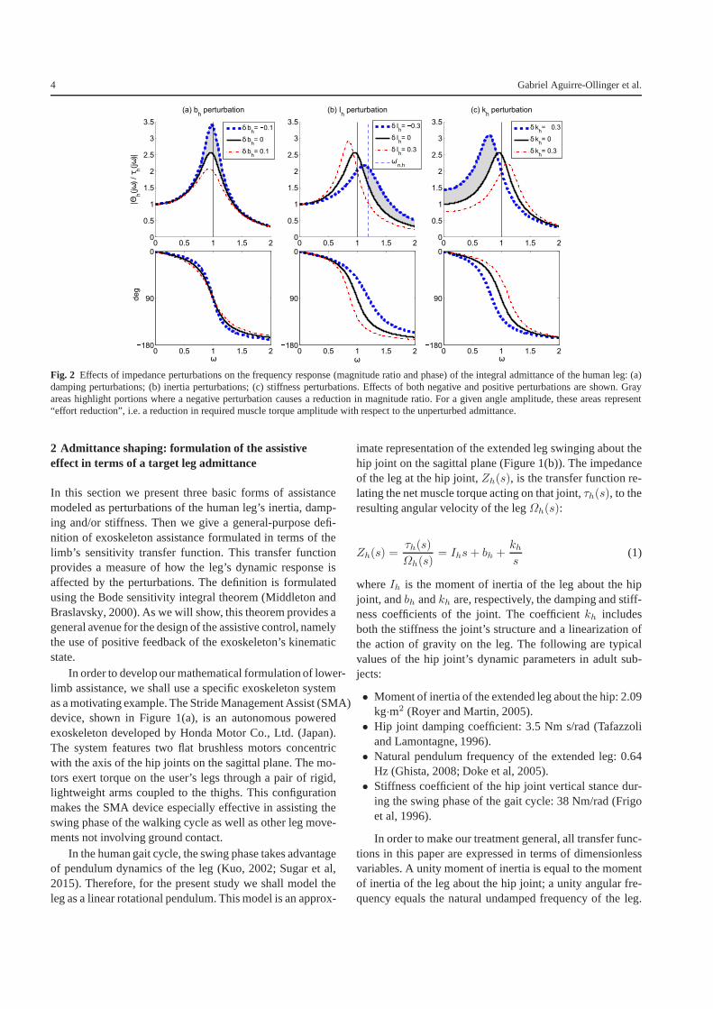
Fig. 2 Effects of impedance perturbations on the frequency response (magnitude ratio and phase) of the integral admittance ofthe human leg: (a)damping perturbations; (b) inertia perturbations; (c) stiffness perturbations. Effects of both negative and positive perturbations are shown. Grayareas highlight portions where a negative perturbation causes a reduction in magnitude ratio. For a given angle amplitude, these areas represent“effort reduction”, i.e. a reduction in required muscle torque amplitude with respect to the unperturbed admittance.
2 Admittance shaping: formulation of the assistiveeffect in terms of a target leg admittance
In this section we present three basic forms of assistancemodeled as perturbations of the human leg’s inertia, damp-ing and/or stiffness. Then we give a general-purpose defi-nition of exoskeleton assistance formulated in terms of thelimb’s sensitivity transfer function. This transfer functionprovides a measure of how the leg’s dynamic response isaffected by the perturbations. The definition is formulatedusing the Bode sensitivity integral theorem (Middleton andBraslavsky, 2000). As we will show, this theorem provides ageneral avenue for the design of the assistive control, namelythe use of positive feedback of the exoskeleton’s kinematicstate.
In order to develop our mathematical formulation of lower-limb assistance, we shall use a specific exoskeleton systemas a motivating example. The Stride Management Assist (SMA)device, shown in Figure 1(a), is an autonomous poweredexoskeleton developed by Honda Motor Co., Ltd. (Japan).The system features two flat brushless motors concentricwith the axis of the hip joints on the sagittal plane. The mo-tors exert torque on the user’s legs through a pair of rigid,lightweight arms coupled to the thighs. This configurationmakes the SMA device especially effective in assisting theswing phase of the walking cycle as well as other leg move-ments not involving ground contact.
In the human gait cycle, the swing phase takes advantageof pendulum dynamics of the leg (Kuo, 2002; Sugar et al,2015). Therefore, for the present study we shall model theleg as a linear rotational pendulum. This model is an approx-
imate representation of the extended leg swinging about thehip joint on the sagittal plane (Figure 1(b)). The impedanceof the leg at the hip joint,Zh(s), is the transfer function re-lating the net muscle torque acting on that joint,τh(s), to theresulting angular velocity of the legΩh(s):
Zh(s) =τh(s)
Ωh(s)= Ihs+ bh +
khs
(1)
whereIh is the moment of inertia of the leg about the hipjoint, andbh andkh are, respectively, the damping and stiff-ness coefficients of the joint. The coefficientkh includesboth the stiffness the joint’s structure and a linearization ofthe action of gravity on the leg. The following are typicalvalues of the hip joint’s dynamic parameters in adult sub-jects:
• Moment of inertia of the extended leg about the hip: 2.09kg·m2 (Royer and Martin, 2005).
• Hip joint damping coefficient: 3.5 Nm s/rad (Tafazzoliand Lamontagne, 1996).
• Natural pendulum frequency of the extended leg: 0.64Hz (Ghista, 2008; Doke et al, 2005).
• Stiffness coefficient of the hip joint vertical stance dur-ing the swing phase of the gait cycle: 38 Nm/rad (Frigoet al, 1996).
In order to make our treatment general, all transfer func-tions in this paper are expressed in terms of dimensionlessvariables. A unity moment of inertia is equal to the momentof inertia of the leg about the hip joint; a unity angular fre-quency equals the natural undamped frequency of the leg.

An admittance shaping controller for exoskeleton assistance of the lower extremities 5
Based on the above published data we set the damping ratioof the hip joint toζh = 0.2. This yields the following valuesfor the coefficients in (1):Ih = 1, bh = 0.4 andkh = 1.
2.1 Shaping the admittance via impedance perturbations
We model the ideal effect of assisting the human limb asapplying an additive perturbationδZh to the limb’s naturalimpedanceZh; the perturbed impedance is simply
Zh = Zh + δZh (2)
An equivalent expression can be given in terms of the leg’sadmittance,Yh(s) = Zh(s)
−1. The perturbed admittance,Yh(s), represents a negative feedback system formed byYh
andδZh:
Yh =1
Zh + δZh
=Yh
1 + YhδZh
(3)
Our task is now to determine what makesδZh assistive, i.e.what kind of perturbation makesYh an improvement overthe leg’s normal admittanceYh. We note that each of the pa-rametersIh, bh andkh contributes to the magnitude of theleg’s impedance (1); therefore we start by studying the ef-fects of compensating each of the leg’s dynamic properties.Accordingly we define the following perturbation types:
δZh = δbh (damping perturbation)
δZh = δIhs (inertia perturbation)
δZh = δkh/s (stiffness perturbation) (4)
Compensationmeans that eitherδbh or δIh or δkh has anegative value. We now analyze the effects the individualperturbations on the frequency response of the integral ad-mittanceYh(s)/s, which relates the net muscle torque to theangular position of the leg. We use this rather than the admit-tance in order to consider possible effects on the “DC gain”(zero-frequency response) as well.
Figure 2 shows the effects of each individual perturba-tion on the leg’s integral admittance. Although our primaryinterest is compensation, we have also plotted the effects ofpositive perturbations for comparison. Examination of theplots reveals several properties of the perturbed frequencyresponses that can be considered asassistance:
• Damping compensationincreases the peak magnitude ofthe integral admittance. In consequence, for given angu-lar trajectories near the natural frequency (ω = 1), theamplitude of the required muscle torque is reduced withrespect to the unperturbed case. We refer to this effect as“effort reduction”.
(a)
(b)
Fig. 3 (a) Block diagram representing the dynamics of the human legin the presence of an impedance perturbationδZh. The perturbed ad-mittance of the leg is equal to the nominal admittanceYh in serieswith a closed-loop system representing the sensitivitySh. (b) Equiva-lent system formed by the human limb coupled to the exoskeleton. TheperturbationδZh is replaced by the exoskeleton transfer functionZe.Per the Bode sensitivity integral theorem, to make the coupled system’ssensitivity larger than the unperturbed case, positive feedback must beused.
• Inertia compensationcauses an increase in the naturalfrequency of the leg with no change in DC gain. In con-sequence, given a desired amplitude of angular motion,the minimum muscle torque amplitude occurs now at ahigher frequency. We hypothesize that the shift in natu-ral frequency has a potential beneficial effects on the gaitcycle. It may enable the user to walk at higher steppingfrequencies without a significant increment in muscleactivation (Doke and Kuo, 2007). A higher natural fre-quency also implies a quicker transient response, whichmay enable the user to take quicker reactive steps whentrying to avoid a fall.
• Stiffness compensationproduces effort reduction at fre-quencies below the natural frequency.
Each case has also its drawbacks. For example, the effectof damping compensation vanishes as motion frequency de-parts from the natural frequency. Inertia compensation causeseffort increase at frequencies immediately below the naturalfrequency. However, by applying the principle of superposi-tion, it is possible to devise a perturbation transfer functionthat combines the beneficial aspects of each individual per-turbation. In other words, the resulting integral admittancecan simultaneously feature increases in natural frequency,magnitude peak and DC gain with respect to the unassistedone.
As for perturbations involving positive values ofδbh,δIh and/orδkh, we refer to these asresistiveto indicate thatthey mainly tend to reduce the leg’s mobility.
6 Gabriel Aguirre-Ollinger et al.
0 1 2 3 4
−0
−0
−0
0
0
0
0
ω
ln|S
h(jω
)|
(a) bh
perturbation
δbh= −0
δbh= 0
δbh= 0
0 1 2 3 4
−0
−0
−0
0
0
0
0
ω
(b) Ih
perturbation
δIh= −0
δIh= 0
δIh= 0
0 1 2 3 4
−0
−0
−0
0
0
0
0
ω
(c) kh
perturbation
δkh= −0
δkh= 0
δkh= 0
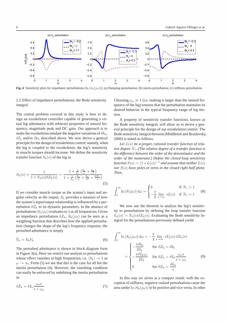
Fig. 4 Sensitivity plots for impedance perturbations (ln |Sh(jω)|). (a) Damping perturbation; (b) inertia perturbation; (c)stiffness perturbation.
2.2 Effect of impedance perturbations: the Bode sensitivityintegral
The central problem covered in this study is how to de-sign an exoskeleton controller capable of generating a vir-tual leg admittance with arbitrary properties of natural fre-quency, magnitude peak and DC gain. Our approach is tomake the exoskeleton emulate the negative variations ofδbh,δIh and/orδkh described above. We now derive a generalprinciple for the design of exoskeleton control: namely, whenthe leg is coupled to the exoskeleton, the leg’s sensitivityto muscle torques should increase. We define the sensitivitytransfer functionSh(s) of the leg as
Sh(s) =1
1 + Yh(s)δZh(s)=
1 + 1
Ih
(bhs+ kh
s2
)
1 + 1
Ih
(bhs+ kh
s2+ δZh
s
)
(5)
If we consider muscle torque as the system’s input and an-gular velocity as the output,Sh provides a measure of howthe system’s input/output relationship is influenced by a per-turbationδZh to its dynamic parameters. In the absence ofperturbationsSh(jω) evaluates to 1 at all frequencies. Givenan impedance perturbationδZh, Sh(jω) can be seen as aweighting function that describes how the applied perturba-tion changes the shape of the leg’s frequency response; theperturbed admittance is simply
Yh = ShYh (6)
The perturbed admittance is shown in block diagram formin Figure 3(a). Here we restrict our analysis to perturbationswhose effect vanishes at high frequencies, i.e.|Sh| → 1 asω → ∞. From (5) we see that this is the case for all but theinertia perturbation (4). However, the vanishing conditioncan easily be enforced by redefining the inertia perturbationas
δZh = δIhωos
s+ ωo
(7)
Choosingωo ≫ 1 (i.e. making it larger than the natural fre-quency of the leg) ensures that the perturbation maintains itsdesired behavior in the typical frequency range of leg mo-tion.
A property of sensitivity transfer functions, known asthe Bode sensitivity integral, will allow us to derive a gen-eral principle for the design of our exoskeleton control. TheBode sensitivity integral theorem (Middleton and Braslavsky,2000) is stated as follows:
LetL(s) be a proper, rational transfer function of rela-tive degreeNr. (The relative degree of a transfer function isthe difference between the order of the denominator and theorder of the numerator.) Define the closed-loop sensitivityfunctionS(s) = (1+L(s))−1 and assume that neitherL(s)nor S(s) have poles or zeros in the closed right half plane.Then,
∫ ∞
0
ln |S(jω)| dω =
0 if Nr > 1
−π
2lims→∞
sL(s) if Nr = 1(8)
We now use the theorem to analyze the leg’s sensitiv-ity to perturbations by defining the loop transfer functionLh(s) = Yh(s)δZh(s). Evaluating the Bode sensitivity in-tegral for the perturbations previously defined yields
∫ ∞
0
ln |Sh(jω)| dω = −π
2lims→∞
sYh(s) δZh(s)
=
−πδbh2Ih
for δZh = δbh
−πδIhωo
2Ihfor δZh = δIh
ωos
s+ ωo
0 for δZh =δkhs
(9)
In this way we arrive at a compact result: with the ex-ception of stiffness,negative-valuedperturbations cause thearea underln |Sh(jω)| to bepositiveand vice versa. In other
An admittance shaping controller for exoskeleton assistance of the lower extremities 7
words, assistive perturbations cause a net increase in sensi-tivity, whereas resistive perturbations cause a net decrease1.To illustrate these points, Figure 4 shows plots ofln |Sh(jω)|
vs.ω for the different types of perturbation.
2.3 Generating assistive impedance perturbations with anexoskeleton: considerations for control
In (3) the perturbed admittance is represented as the cou-pling of two dynamical systems: the leg’s original admit-tanceYh, and the impedance perturbationδZh. Given thatwe want to design a controller for the coupled system formedby the leg and the exoskeleton, (3) suggests a simple designstrategy: substituteδZh with the exoskeleton’s port impe-dance,Ze(s). The task is to design a control to makeZe(s)
emulate the behavior ofδZh as closely as possible.The sensitivity transfer function of the coupled system
formed by the leg and the exoskeleton is
She(s) =1
1 + Yh(s)Ze(s)(10)
and its loop transfer function isLhe(s) = Yh(s)Ze(s). Forthe coupled system to emulate assistive (i.e. negative) per-turbations of inertia or damping, the Bode sensitivity inte-gral of She(s) must be positive. From (8) the only way toaccomplish this is by making the gain ofZe(s) negative. Inother words, the exoskeleton has to form apositive feedbackloop with the human leg, as shown in Figure 3(b).
An important consequence of the gain being negative isthat the exoskeleton displaysactivebehavior, i.e. acts as anenergy source, which in turn raises the issue of coupled sta-bility. Colgate and Hogan (1988) have shown that a manip-ulator is guaranteed remain stable, when coupled to an ar-bitrary passive environment, if the manipulator itself is pas-sive. However, passive behavior can seriously limit perfor-mance (Hogan and Buerger, 2006). In the case of an exoske-leton, passive behavior would render it incapable of provid-ing true assistance, at least per the criteria we have outlinedin Section 2.1.
But then, our requirement is not to ensure stable interac-tion with every possible passive environment, but only witha certain class of environments, namely those possessing thetypical dynamic properties of the human leg. Limiting theset of passive environments with which the exoskeleton isintended to interact allows us, in turn, to use a less restrictivestability criterion. For example, stability can be guaranteedby the Bode criterion for positive feedback:
| − Yh(jω)Ze(jω)| < 1
where ∠ (−Yh(jω)Ze(jω)) = −180(11)
1 For stiffness perturbations the area underln |Sh(jω)| remains con-stant, meaning that if the sensitivity increases in one frequency range,it will be attenuated in the same proportion elsewhere.
In the next section we present the formulation of a stableassistive controller capable of generating a virtual leg admit-tance with arbitrary values of natural frequency, magnitudepeak and, for the integral admittance, DC gain.
3 Lower-limb assistance by admittance shaping: controldesign
3.1 Specifying a target frequency response for the leg
We shall base our control design specifications on the humanlimb’s integral admittance,Xh(s) ≡ Yh(s)/s, expressed interms of dynamic response parameters:
Xh(s) =1
Ih(s2 + 2ζhωnhs+ ω2
nh)(12)
whereωnh is the natural frequency of the leg andζh itsdamping ratio. Our design objective is to make the assistedleg behave in accordance with atarget integral admittancemodelXd
h(s), defined as
Xdh(s) =
1
Idh(s2 + 2ζdhω
dnhs+ ωd 2
nh )(13)
whereIdh , ωdnh andζdh are, respectively, the desired values of
inertia moment, natural frequency and damping ratio. Thedesign specifications are formulated in terms of the follow-ing parameter ratios:
Rω ≡ωdnh
ωnh
(natural frequencies ratio) (14)
RM ≡Md
h
Mh
(resonant peaks ratio) (15)
RDC ≡Xd
h(0)
Xh(0)(DC gains ratio) (16)
In (15)Mh andMdh are, respectively, the magnitude peaks at
resonance forXh(jω) andXdh(jω). Thus our design spec-
ifications consist of desired values forRω, RM andRDC .These specifications are converted into desired values for thedynamic parametersIdh , ωd
nh, ζdh by using the following for-mulas, which are derived in Appendix A:
Idh =Ih
RDCR2ω
(17)
ωdnh = Rωωnh (18)
ζdh =
√1−
√1− 4ρ2
2(19)

8 Gabriel Aguirre-Ollinger et al.
Rω R
M R
D
ωn
ωn
d
Xh(
Xh
(
h
h
Xh(jω)
X dh(jω)
−
−1
−
−1
ω
ωn ω
n
d
ang(Xh(jω))
ang(X dh(jω))
Fig. 5 Frequency responses of the unassisted leg’s integral admittanceXh(jω) and an exemplary target integral admittanceXd
h(jω) with
Rω = 1.2,RM = 1.4 andRDC = 1.4. The computed parametersfor Xd
h(jω) areId
h= 0.4960,ωd
nh= 1.2 andζd
h= 0.1989.
Fig. 6 Linear model of the system formed by the human leg, couplingand exoskeleton mechanism.
where
ρ =RDC
RM
ζh
√1− ζ2h (20)
By way of example, Figure 5 shows a comparison be-tween the frequency responses of the unassisted leg’s in-tegral admittanceXh(jω) and a target integral admittanceXd
h(jω) with specific values ofRω, RM andRDC . Thisparticular target response combines all the possible assis-tive effects on the leg: increase in natural frequency, effortreduction at resonance, and gravitational support at low fre-quencies.
Our task is now to design an exoskeleton control capableof making the leg’s dynamic response emulate the targetXd
h.
3.2 Modeling the coupled human-exoskeleton system
To design the exoskeleton control we shall use the linearizedmodel shown in Figure 6, which represents the human legcoupled to the exoskeleton’s arm-actuator assembly (Figure1(a)). The inertias of the leg and the exoskeleton are coupledby a spring and damper (kc, bc) representing the complianceof the leg muscle tissue combined with the compliance of the
exoskeleton’s thigh brace. In the diagram, ground representsthe exoskeleton’s hip brace and is assumed to be rigid.
The first design goal is to make the device’s mecha-nism “transparent” when the assistive function is inactive. Inother words, the user should feel the effects the mechanism’sdynamics (inertia, friction, gravitational effects) as little aspossible (Vallery et al, 2009a). This normally requires im-plementing an inner-loop control, such as an admittance orimpedance control, to compensate the reflected inertia, fric-tion and damping of the mechanism, as well as the gravita-tional torques (Nef et al, 2007). The maximum achievablereduction in reflected inertia is limited by stability bound-aries (Colgate and Hogan, 1989a); therefore it is advisableto employ a mechanism design that uses low-inertia compo-nents. In the present formulation we will assume that suchan inner-loop control is already in place, thereby allowingusto represent the exoskeleton arm as a pure rotational inertia:Ze(s) = Ies.
We note that the exoskeleton and the compliant couplingcan be represented as second-order impedance given by
Zec(s) = Ies+ bc +kcs
(21)
or, equivalently,
Zec(s) = Ie
(s+ 2ζecωn,ec +
ω2
n,ec
s
)(22)
whereωn,ec is the natural frequency of the impedance andζec its damping ratio. The value ofωn,ec depends on a num-ber of factors like the material of the exoskeleton’s thighcoupling and the properties of the subject’s thigh tissue. Fromour system identification studies, values ofωn,ec in the rangeof 25 to 50 times the natural frequency of the leg (ωnh) aretypical for the SMA device. In order to reduce the dimen-sionality of the analysis somewhat, we assume the impe-dance (22) to be critically damped, i.e.ζec = 1. This as-sumption is warranted because our tests with the SMA haveshownZec(s) to be actually overdamped, so the critically-damped assumption is conservative as far as stability is con-cerned. Keeping our analysis in terms of dimensionless fre-quencies and damping ratios, we define the following impe-dance transfer functions:
Zh(s) = Y −1
h (s) =s2 + ζhs+ 1
s(23)
Zc(s) = Y −1
c (s) = 2Ieωn,ec
(s+
ωn,ec
2
s
)(24)
Ze(s) = Y −1
e (s) = Ies (25)
We use these impedances to formulate the dynamics equa-tions of the coupled human-exoskeleton system of Figure 6

An admittance shaping controller for exoskeleton assistance of the lower extremities 9
(a)
(b)
(c)
Fig. 7 Block diagrams of the system formed by the human leg, cou-pling, exoskeleton mechanism and interaction controller.(a) Block dia-gram derived from equations (26) to (29). (b) Equivalent block diagramfor control design. The transfer functionYhecf (s) = Ωe(s)/τh(s)represents the admittance of the human leg assisted by the exoskele-ton. (c) Equivalent block diagram for stability robustnessanalysis.
in the Laplace domain (the derivation is omitted due to spacelimitations):
Ωh = Yh (τh − τc) (26)
τc = Zc (Ωh −Ωe) (27)
Ωe = Ye (τc − τe) (28)
whereτc is the interaction torque between the leg and theexoskeleton (exerted through the coupling) andτe is the torquegenerated by a feedback compensatorZf (s):
τe = Zf Ωe (29)
Zf (s) embodies the exoskeleton’s assistive action.It shouldbe noted that, although the compensator takes in angular ve-locity feedback,Zf (s) may contain derivative or integralterms. Therefore the physical control implementation mayinvolve feedback of angular acceleration or angular position.Another observation is that, although the torque generatedby the control isτe, the actual torque exerted on the leg bythe exoskeleton isτc.
3.3 Design of the assistive control
Using equations (26), (27), (28) and (29), we represent thecoupled leg-exoskeleton system as the block diagram of Fig-ure 7(a). The aim of the assistive control is to make thedynamic response of this system such that it matches thefrequency response of the target integral admittanceXd
h(s).Our control design method is a two-step procedure:
• Design of an angle feedback compensator to achieve thetarget DC gain (stiffness and gravity compensation).
• Design of an angular acceleration feedback compensatorto achieve the target natural frequency and target reso-nant peak. This second compensator is designed using apole placement technique and has to ensure the stabilityof the coupled system.
Decoupling the DC gain problem from the other two isvalid because, as can be seen on Figure 2, the DC gain isonly affected by a stiffness perturbation, which is easily im-plemented via angle feedback. The same figure suggests thatthe natural frequency target could be achieved by either an-gle feedback (stiffness perturbation) or angular accelerationfeedback (inertia perturbation). By choosing angular accel-eration feedback we avoid creating a conflict with the DCgain objective, which depends exclusively on angle feed-back. Furthermore, we will show that employing an angularacceleration feedback compensator with sufficient degreesof freedom allows us to achieve the natural frequency andresonant peak targets simultaneously.
3.3.1 Feedback compensator for target DC gain
The design of the compensator for target DC gain is a simpleapplication of the dynamics of the coupled system in thestatic (zero frequency) case. From Figure 6, torque balanceon the human leg’s inertiaIh yields
khθh = τh − τc (30)
Torque balance on the exoskeleton’s inertiaIe yields
τc − τe = 0 (31)
Because the objective is to compensate for the stiffness andgravitational torque acting on the leg, the assistive torque isprovided by a virtual spring:
τe = kDCθe (32)
Assuming the coupling to have sufficient stiffness so thatθe ≃ θh, from (30) the net muscle torque becomes
τh = khθh − kDCθe ≃ (kh − kDC)θh (33)
10 Gabriel Aguirre-Ollinger et al.
To determine the virtual spring stiffnesskDC we refer toAppendix A. Equation (79) defines an intermediate targetintegral admittanceXh,DC(s) embodying the DC gain spec-ification. Maintaining the assumptionθe ≃ θh we note thatXh,DC(s) can be implemented by adding the virtual springto the human leg’s impedance. Thus an alternative definitionis
Xh,DC(s) =1
Ihs2 + 2Ihζhωnhs+ Ihω2
nh + kDC
(34)
MakingXh,DC(0) = Xh,DC(0) yields
Ihω2
nh + kDC = Ihω2
nh,DC (35)
But from (81) we haveω2
nh,DC = R−1
DCω2
nh. Thus we obtainthe stiffness and gravity compensation gain as:
kDC = Ihω2
nh(R−1
DC − 1) (36)
The angular position feedback (32) with the computed valueof kDC generates the following closed-loop exoskeleton ad-mittance:
Ye,DC =Ye
1 +kDC
sYe
(37)
Clearly, for a DC gain specification ofRDC > 1 we havekDC < 0, i.e. positive feedback of the angular position. Inconsequence, the closed-loop exoskeleton admittance has apole ats = +
√kDC I−1
e , which makes the isolated exoske-leton unstable. However, the coupled system formed by theleg and the exoskeleton will be stable as long as the virtualstiffness coefficient of the assisted leg remains positive.Adetailed analysis of the stability of the coupled system withDC gain compensator is given in the next section.
3.3.2 Loop transfer function of the coupled human limband exoskeleton
With the compensator for the target DC gain already in place,the forthcoming analysis will focus on thetarget admittancefor the assisted leg, given byY d
h (s) = sXdh(s). The objec-
tive is now to design a compensator capable of increasingthe natural frequency of the leg as well as the magnitudepeak of its admittance. This is also the more involved part ofour control design, since we need to design for both perfor-mance and stability. Although, strictly speaking, we want tocontrol the relationship between the human muscle torqueτh and the leg’s angular velocityΩh as to matchY d
h (s), ourdesign will focus on the transfer function relatingτh to theexoskeletonangular velocityΩe, the reason being that we
only have a practical way of measuringΩe. This is accept-able under the assumption that the coupling is sufficientlyrigid and thereforeΩe ≃ Ωh.
We begin by substitutingYe(s) with Ye,DC(s) in Fig-ure 7(a) and converting the block diagram to a form suitablefor analysis using the system’s loop transfer function. Figure7(b) shows the equivalent block diagram (derivation omittedfor brevity), which contains the following transfer functions:
Yhec(s) =Zh + Zc
ZhZe,DC + ZcZe,DC + ZcZh
≡Nhec(s)
Dhec(s)
(38)
whereZe,DC = Y −1
e,DC , and
Hhc(s) =Zc
Zh + Zc
=Zc
Nhec(s)(39)
From Figure 7(b) we derive the transfer function relating thehuman torque to the encoder angular velocity:
Yhecf (s) =Ωe(s)
τh(s)=
Zc
Dhec + ZfNhec
(40)
Yhecf (s) is very important in our analysis because it repre-sents the admittance of the human leg assisted by the exo-skeleton. From linear feedback control theory, the dynamicresponse properties ofYhecf (s) are determined mainly byits characteristic polynomial. Therefore we shall formulatethe design of the compensatorZf (s) as a pole placementproblem: namely, to make thedominant polesof Yhecf (s)
match the poles of the target admittanceY dh (s). Our design
will use the standard tools of root locus and Bode stabilityapplied to the loop transfer function ofYhecf (s).
From Figure 7(b), we define the loop transfer function,Lhecf(s), as a ratio of monic polynomials obeying
KLLhecf(s) = Zf(s)Yhec(s) (41)
whereKL is the loop gain. Success in the design of the feed-back compensatorZf (s) requires ensuring that the feed-back loop formed byZf (s) andYhec(s) is stable. Given thatYhec(s) already contains a positive feedback loop of the an-gular position (throughZe,DC ), we want to analyze its sta-bility properties before designingZf (s). For the forthcom-ing analysis we shall use the dimensionless moment of in-ertia of the SMA arm and actuator assembly,Ie = 0.00702.We begin by writing the impedances in (38) in terms of poly-nomial ratios and gains:

An admittance shaping controller for exoskeleton assistance of the lower extremities 11
2
2
1
2
3
1.2
1
2
-2
DCωn,ec
1
0.8
0.6
0.4
0.2
0
-0.2
Fig. 8 Contour plot showing the real part of the dominant poles ofYhec(s) (equation (43)) as a function of the DC gain ratioRDC andthe coupling’s natural frequency,ωn,ec.
Zh(s) =s2 + ζhs+ 1
s≡
Nh(s)
s
Zc(s) = 2Ieωn,ec
(s+
ωn,ec
2
s
)≡ zco
Nc(s)
s
Ze,DC(s) = Ie
(s2 + kDC
Ie
s
)≡ Ie
Ne(s)
s(42)
This, in turn, allows us to writeYhec(s) as the followingratio of polynomials:
Yhec(s) =s(Nh + zcoNc)
IeNeNh + zcoNeNc + zcoNh
(43)
From inspection of (42) and (43) we find thatYhec(s) hasfour poles and three zeros, including one zero at the origin.
Figure 8 shows contour plots of the real part of the dom-inant poles ofYhec(s) as a function of the DC gains ratioRDC and the natural frequency of the couplingωn,ec. Thesepoles are located near the poles of the human leg’s admit-tance,−0.2± 0.980j. We can observe that, for most valuesof RDC andωn,ec, the dominant poles’ real part is constantand equal to−0.2, i.e. the dominant poles are stable. Onlyfor combinations of very low natural frequency of the cou-pling and high DC gain ratios do the dominant poles crossover to the right-hand side of the complex plane (RHP). Fornow we will maintain the assumption that theRDC spec-ification is such that does not violate the stability ofYhec.Ensuring thatYhec has no RHP or imaginary poles guaran-tees the existence of a range of negative loop gainsKL forwhich the closed-loop transfer functionYhecf (s) is stable aswell.
3.3.3 Feedback compensator for target values of naturalfrequency and resonant peak: design by pole placement
In order to explain the derivation of the feedback compen-satorZf (s) for natural frequency and resonant peak targets,we will use a specific design example involving the HondaSMA device. We set forth the following design specifica-tions:Rω = 1.2,RM = 1.3 andRDC = 1.1, which in turnyield the following parameter values for the target integraladmittance (13):Idh = 0.631,ωd
nh = 1.2 andζdh = 0.1673.Given these values, the desired locations of the dominantpoles are
pdh = −σdh + jωd
dh = −0.201+ 1.183j
pdh = −σdh − jωd
dh = −0.201− 1.183j
where
σdh = ζdhω
dnh
ωddh = ωd
nh
√1− ζd 2
h (44)
The gain of the feedback compensator for target DC gainis computed with (36), yieldingkDC = −0.0909.
In Section 2.1 we showed that, in the ideal case, an in-crease in natural frequency can be accomplished by com-pensating the second-order system’s inertia. This suggeststhat our compensator should include positive accelerationfeedback in some form. Although pure acceleration feed-back will not satisfy our design requirements, it is nonethe-less instructive to examine its behavior. Thus we define theprovisional compensator
Zf(s) ≡ −Ics (45)
We shall refer toIc as the inertia compensation gain. Thenwe write
Zf(s)Yhec(s) = −IcIe
sLhec (46)
whereLhec(s) is a ratio of monic polynomials possessingthe same poles and zeros asYhec(s). From (46) the loopgain for pure acceleration feedback as
KL = −IcIe
(47)
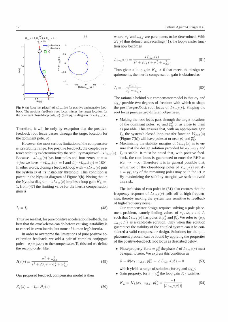
Figure 9(a) shows the root loci ofsLhec(s) for both pos-itive and negative feedback. Because all the coefficients ofsLhec(s) are fixed, the shape of the root loci is constant andthe only variable parameter we have is the loop gainKL.
12 Gabriel Aguirre-Ollinger et al.
−1 − 0
0
1
2
Re(s)
Im(s
)
(a)Rωn
= 1.2, RM
= 1.3, RDC
= 1.1,
ωn,c
= 25
−1 −0.5 0 0.5 1
−1
−0.5
0
0.5
1
Re[ jωLhec
(jω) ]
Im[
jωL
he
c(jω
) ]
(b)
(+) feedback
(−) feedback
ph
d
Fig. 9 (a) Root loci (detail) ofsLhec(s) for positive and negative feed-back. The positive-feedback root locus misses the target location forthe dominant closed-loop pole,pd
h. (b) Nyquist diagram for -sLhec(s).
Therefore, it will be only by exception that the positive-feedback root locus passes through the target location forthe dominant pole,pdh.
However, the most serious limitation of the compensatoris its stability range. For positive feedback, the coupled sys-tem’s stability is determined by the stability margins of−sLhec(s).Because−sLhec(s) has four poles and four zeros, ats =
+j∞we have|−sLhec(s)| = 1 and∠(−sLhec(s)) = 180.In other words, closing a feedback loop with−sLhec(s) putsthe system is at its instability threshold. This condition ispatent in the Nyquist diagram of Figure 9(b). Noting that inthe Nyquist diagram−sLhec(s) implies a loop gainKL =-1, from (47) the limiting value for the inertia compensationgain is
Ic = Ie (48)
Thus we see that, for pure positive acceleration feedback, thebest that the exoskeleton can do before causing instabilityisto cancel its own inertia, but none of human leg’s inertia.
In order to overcome the limitations of pure positive ac-celeration feedback, we add a pair of complex conjugatepoles−σf±jωd,f to the compensator. To this end we definethe second-order filter
Hf (s) ≡σ2
f + ω2
d,f
s2 + 2σfs+ σ2
f + ω2
d,f
(49)
Our proposed feedback compensator model is then
Zf (s) ≡ −Ic sHf(s) (50)
whereσf andωd,f are parameters to be determined. WithZf(s) thus defined, and recalling (41), the loop transfer func-tion now becomes
Lhecf(s) =sLhec(s)
s2 + 2σfs+ σ2
f + ω2
d,f
(51)
Thus given a loop gainKL < 0 that meets the design re-quirements, the inertia compensation gain is obtained as
Ic = −KL Ie
σ2
f + ω2
d,f
(52)
The rationale behind our compensator model is thatσf andωd,f provide two degrees of freedom with which to shapethe positive-feedbackroot locus ofLhecf (s). Shaping theroot locus pursues two different objectives:
• Making the root locus pass through the target locationsof the dominant poles,pdh and pdh or as close to themas possible. This ensures that, with an appropriate gainIc, the system’s closed-loop transfer functionYhecf (s)(Figure 7(b)) will have poles at or nearpdh andpdh.
• Maximizing the stability margins ofYhecf (s) as to en-sure that the design solution provided byσf , ωd,f andIc is stable. It must be noted that, with positive feed-back, the root locus is guaranteed to enter the RHP asKL → −∞. Therefore it is in general possible that,while two of the closed-loop poles ofYhecf (s) satisfys = pdh, any of the remaining poles may be in the RHP.By maximizing the stability margins we seek to avoidthis risk.
The inclusion of two poles in (51) also ensures that thefrequency response ofLhecf (s) rolls off at high frequen-cies, thereby making the system less sensitive to feedbackof high-frequency noise.
Our compensator design requires solving a pole place-ment problem, namely finding values ofσf , ωd,f and Icsuch thatYhecf (s) has poles atpdh andpdh. We refer toσf ,ωd,f , Ic as a candidate solution. Only when this solutionguarantees the stability of the coupled system can it be con-sidered a valid compensator design. Solutions for the poleplacement problem can be found by applying the propertiesof the positive-feedback root locus as described below.
• Phase property: fors = pdh the phaseΦ of Lhecf (s) mustbe equal to zero. We express this condition as
Φ = Φ(σf , ωd,f , pdh) = ∠Lhecf(p
dh) = 0 (53)
which yields a range of solutions forσf andωd,f .• Gain property: fors = pdh the loop gainKL satisfies
KL = KL(σf , ωd,f , pdh) =
−1
|Lhecf (pdh)|(54)
An admittance shaping controller for exoskeleton assistance of the lower extremities 13
−8 −6 −4 −2
0.5
1
1.5
2
2.5
3
3.5
4
11.21.
31.41.
5
1.6
1.7
−σf
1.8
ωn,ec
= 100 (R
ω n = 1.2, R
M = 1.3, R
DC = 1.1)
1.9
2
ωd,
f
−8 −6 −4 −2
0.5
1
1.5
2
2.5
3
3.5
4
11.21.
31.41.
5
1.6
1.7
1.8
1.9
2
ωn,ec
= 50
−σf
1.91.
11
0.9
ωd,
f
−8 −6 −4 −2
0.5
1
1.5
2
2.5
3
3.5
4 1
1.8
1.2
1.4
1.6
10.8
ωn,ec
= 25
−σf
0.60.
4
0.3
ωd,
f
−8 −6 −4 −2
0.5
1
1.5
2
2.5
3
3.5
4
0.2
0.1
ωn,ec
=10
−σf
0.06
0.04
ωd,
f
Φ = 0, RIc
> 1
RIc
= 2.038
Φ = 0, RIc
> 1
RIc
= 2.281
Φ = 0, RIc
> 1
RIc
= 1.95
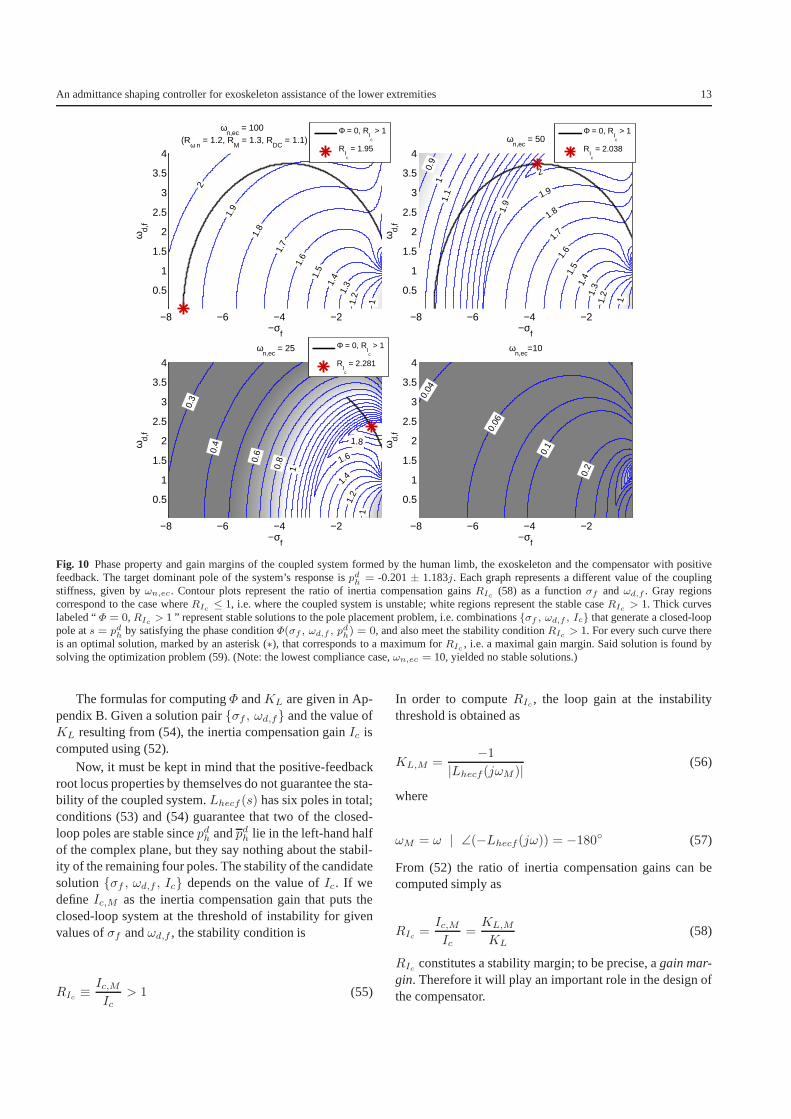
Fig. 10 Phase property and gain margins of the coupled system formedby the human limb, the exoskeleton and the compensator with positivefeedback. The target dominant pole of the system’s responseis pd
h= -0.201± 1.183j. Each graph represents a different value of the coupling
stiffness, given byωn,ec. Contour plots represent the ratio of inertia compensationgainsRIc (58) as a functionσf andωd,f . Gray regionscorrespond to the case whereRIc ≤ 1, i.e. where the coupled system is unstable; white regions represent the stable caseRIc > 1. Thick curveslabeled “Φ = 0,RIc > 1 ” represent stable solutions to the pole placement problem, i.e. combinationsσf , ωd,f , Ic that generate a closed-looppole ats = pd
hby satisfying the phase conditionΦ(σf , ωd,f , p
dh) = 0, and also meet the stability conditionRIc > 1. For every such curve there
is an optimal solution, marked by an asterisk (∗), that corresponds to a maximum forRIc , i.e. a maximal gain margin. Said solution is found bysolving the optimization problem (59). (Note: the lowest compliance case,ωn,ec = 10, yielded no stable solutions.)
The formulas for computingΦ andKL are given in Ap-pendix B. Given a solution pairσf , ωd,f and the value ofKL resulting from (54), the inertia compensation gainIc iscomputed using (52).
Now, it must be kept in mind that the positive-feedbackroot locus properties by themselves do not guarantee the sta-bility of the coupled system.Lhecf (s) has six poles in total;conditions (53) and (54) guarantee that two of the closed-loop poles are stable sincepdh andpdh lie in the left-hand halfof the complex plane, but they say nothing about the stabil-ity of the remaining four poles. The stability of the candidatesolutionσf , ωd,f , Ic depends on the value ofIc. If wedefineIc,M as the inertia compensation gain that puts theclosed-loop system at the threshold of instability for givenvalues ofσf andωd,f , the stability condition is
RIc ≡Ic,MIc
> 1 (55)
In order to computeRIc , the loop gain at the instabilitythreshold is obtained as
KL,M =−1
|Lhecf(jωM )|(56)
where
ωM = ω | ∠(−Lhecf(jω)) = −180 (57)
From (52) the ratio of inertia compensation gains can becomputed simply as
RIc =Ic,MIc
=KL,M
KL
(58)
RIc constitutes a stability margin; to be precise, again mar-gin. Therefore it will play an important role in the design ofthe compensator.

14 Gabriel Aguirre-Ollinger et al.
−21 −Res
−30 −29
0
0.5
1
1.5
2
2.5
3
3.5
4
4.5
5
Ims
Rωn
= 1.2, RM
= 1.3, RDC
= 1.1, ωn,c
= 25, Ic
= 0.3156
−2 −1 0 1 2 3 4 5
Res
Ims
−0.3 −0.2 −0.1 0
0.9
1
1.1
1.2
1.3
ζh
ωnh
ph
d
//
////
Fig. 11 Human-exoskeleton system with feedback compensator optimized for the design specifications of Section 3.3.3. Plot shows the positive-feedback root locus of the loop transfer functionLhecf (s). Coupling stiffness isωn,ec = 25. Dashed portions of the root locus correspond to loopgains greater in magnitude than the computed valueKL (93). The inset shows how the root locus passes exactly through the target location of thedominant pole,pd
h; curves corresponding to the damping ratioζh and the natural frequencyωnh of the unassisted leg are shown for comparison.
At this point we need to consider that the values of thesystem’s parameters involve considerable uncertainty, espe-cially in the case of the human leg and the coupling. Asidefrom its implications on performance, parameter uncertaintyposes the risk of instability. Thus the physical coupled sys-tem could be unstable even though the compensator is theo-retically stabilizing. To minimize that risk, we propose for-mulating the design of the compensator as a constrainedoptimization problem: given the target dominant poles =
pdh, to find a combinationσf , ωd,f , Ic that maximizes theinertia compensation gains ratioRIc while preserving thephase condition (53).
To test the feasibility of this approach, we computed thevalues ofΦ(σf , ωd,f , p
dh) andRIc for a matrix of values
of σf andωd,f and with different values of coupling stiff-nessωn,ec as a parameter. The results are shown in Figure10. Contour plots represent constant values ofRIc ; valuesof RIc greater than unity (indicated by white regions in theplot) represent a stable coupled system. The thicker curveslabeled “Φ = 0, RIc > 1 ” are loci of stablesolutionsσf , ωd,f , Ic to the pole placement problem, i.e. solutionsthat simultaneously satisfy the phase conditionΦ(σf , ωd,f , p
dh) =
0 and the stability conditionRIc > 1. As to why the com-pensator is capable of generating stable solutions, the gen-eral principle is given in Section 3.4 with the aid of an ex-ample.
Inspection of the contour plots forRIc shows that foreach stable solution curve it is possible to find a maximumfor RIc . We also notice that the solution curves tend to con-tract and finally disappear asωn,ec decreases, which showsthatωn,ec has an important influence on the stability robust-ness of the assistive control.
Thus we formulate the feedback compensator design prob-lem as follows: given a target dominant polepdh, find
maxσf , ωd,f
R2
Ic(σf , ωd,f , p
dh)
subject to Φ(σf , ωd,f , pdh) = 0 (59)
The complete design procedure of the assistive controlfor admittance shaping is summarized thus:
1. Formulate the design specificationsRω, RM andRDC .2. With the DC gain specificationRDC , compute the angu-
lar position feedback gainkDC using (36).3. Compute the target admittance parametersωd
nh andζdhusing (18) and (19).
4. Obtain the dominant pole of the target admittance aspdh = −σd
h + jωddh using (44).
5. Obtain the parametersσf , ωd,f of the feedback com-pensatorZf (s) (49),(50) by performing the constrainedoptimization (59).
6. With σf , ωd,f obtain the the loop gainKL using (93)and the inertia compensation gainIc using (52).
An admittance shaping controller for exoskeleton assistance of the lower extremities 15
−1 ! 1
−1
!
1
"#$%cs Y
hec(s) H
f(s)
ImI
cs Y
he
c(s
) H
f(s)
(c)
−40 −20 0−30
−20
−10
0
10
20
30
ImI
cs Y
he
c(s
)
(a)
ReIcs Y
hec(s)
10−2
100
102
(b)
Ics Y
hec(s)
Hf(s)
Ics Y
hec(s) H
f(s)
10−1
100
101
102
−180
0
180
360
ω
deg
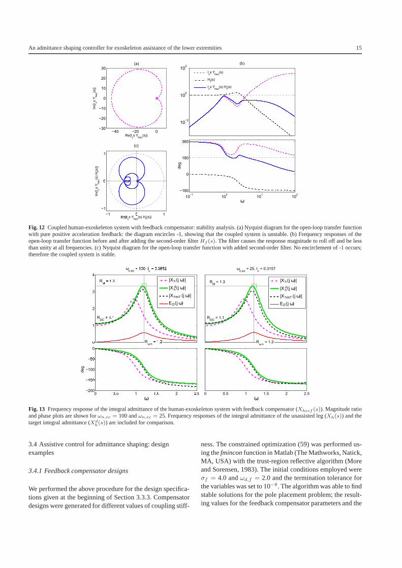
Fig. 12 Coupled human-exoskeleton system with feedback compensator: stability analysis. (a) Nyquist diagram for the open-loop transfer functionwith pure positive acceleration feedback: the diagram encircles -1, showing that the coupled system is unstable. (b) Frequency responses of theopen-loop transfer function before and after adding the second-order filterHf (s). The filter causes the response magnitude to roll off and be lessthan unity at all frequencies. (c) Nyquist diagram for the open-loop transfer function with added second-order filter. No encirclement of -1 occurs;therefore the coupled system is stable.
&
1
2
3
4
ωn,ec
' )&&* +c' &,.//3
Rωn
' ),3
R4' ),.
RDC
' ),)
|Xh(jω)|
|X dh(jω)|
|Xhecf (jω)|
EΩ(jω)
0 &,5 1 ),5 2 3,5−200
−)5&
−100
−5&
0
ω
deg
ωn,ec
= 25, Ic
= 0.3157
Rωn
= 1.2
RM
= 1.3
RDC
= 1.1
|Xh(jω)|
|X dh(jω)|
|Xhecf (jω)|
EΩ(jω)
0 0.5 1 1.5 2 2.5
ω
Fig. 13 Frequency response of the integral admittance of the human-exoskeleton system with feedback compensator (Xhecf (s)). Magnitude ratioand phase plots are shown forωn,ec = 100 andωn,ec = 25. Frequency responses of the integral admittance of the unassisted leg (Xh(s)) and thetarget integral admittance (Xd
h(s)) are included for comparison.
3.4 Assistive control for admittance shaping: designexamples
3.4.1 Feedback compensator designs
We performed the above procedure for the design specifica-tions given at the beginning of Section 3.3.3. Compensatordesigns were generated for different values of coupling stiff-
ness. The constrained optimization (59) was performed us-ing thefminconfunction in Matlab (The Mathworks, Natick,MA, USA) with the trust-region reflective algorithm (Moreand Sorensen, 1983). The initial conditions employed wereσf = 4.0 andωd,f = 2.0 and the termination tolerance forthe variables was set to 10−8. The algorithm was able to findstable solutions for the pole placement problem; the result-ing values for the feedback compensator parameters and the

16 Gabriel Aguirre-Ollinger et al.
Table 1 Feedback compensator parameters and associated inertiacompensation gains ratio
Parameter ωn,ec = 100 ωn,ec = 50 ωn,ec = 25
σf 7.4877 3.8427 0.8622ωd,f 3.98×10⁻⁵ 3.7292 2.3513Ic 0.3662 0.3627 0.3148
RIc 1.950 2.038 2.281
correspondingRIc values are shown in Table 1. The solu-tions are also shown graphically in Figure 10; each asterisk(∗) represents the optimal values ofσf , ωd,f andRIc for aparticular stiffness valueωn,ec.
Figure 11 shows the positive-feedback root locus ofLhecf (s)
for the coupling withωn,ec = 25. This figure illustrates thefact that it is possible to find compensator solutions thatachieve the pole placement objective, despite the fact thatpositive feedback tends to destabilize the coupled system,as indicated by the incursions of the root locus into the RHPasKL → −∞.
3.4.2 Stability of the coupled system
The stabilizing effect of the second-order filter (49) can beunderstood by comparing once more against pure positiveacceleration feedback. Taking the caseωn,ec = 25 in Table1, it is clear that, if we attempt pure positive accelerationfeedback using the prescribed gainIc, the coupled systemwill be unstable. Figure 12(a) shows the Nyquist diagram ofthe corresponding open-loop transfer function,Ic s Yhec(s).This is the same diagram as Figure 9(b) but scaled in mag-nitude; the plot encircles the critical point -1 as a result.The Bode plot ofIc s Yhec(s) in Figure 12(b) shows thatthe magnitude tends to a maximum≫ 1 asω → +∞. How-ever, this effect is counteracted by the frequency rolloff char-acteristic of the filterHf (s). Adding the filter results in anopen-loop transfer functionIc s Yhec(s)Hf (s) of which themagnitude rolls off as well. As a consequence, the magni-tude never exceeds a value of 1, thereby avoiding any encir-clement of -1.
Figure 12(c) shows the Nyquist diagram for the coupledsystem with the second-order filter in place. It can be seenthat the solution is robust to both phase variations and gainvariations. The only limitation is that the gain margin is fi-nite, whereas the phase margin is infinite. Thus in principleit is possible for the coupled system to maintain stability inspite of discrepancies between the system’s model and theactual properties of the physical leg and exoskeleton.
3.4.3 Performance of the coupled system: frequencyresponse
Our design goal was to make the dynamic response of theexoskeleton-assisted leg match the integral admittance modelXd
h(s) (13) as closely as possible. Figure 13 shows a com-parison between the frequency response of the coupled sys-tem’s integral admittanceXhecf (s) and the response of themodelXd
h(s). The frequency response of the unassisted leg(modeled byXh(s)) is shown as well for reference. It canreadily be seen that the response of the coupled system closelymatches that of the model despite the differences of orderamong the transfer functions (Xd
h(s) only has two poles,whereasXhecf (s) has six poles and four zeros.)
In the next section we examine the stability robustnessof the exoskeleton’s control to variations in the parametersof the coupled system.
4 Stability robustness of the exoskeleton control
4.1 Robustness to stiffness parameters
The present analysis assumes the exoskeleton modelZe tobe accurate and focuses on two system parameters that areparticularly difficult to identify, the stiffness of the humanleg’s joint and the stiffness of the coupling. The passive stiff-ness of the hip joint can be estimated with reasonable ac-curacy under highly controlled conditions (Fee and Miller,2004). However, hip impedance also has reflexive compo-nents due to muscle activation (Schouten et al, 2008). Thestiffness of the coupling between the leg and the exoskele-ton, on its part, depends not only on the thigh brace but alsoon the compliance of the thigh tissue, which is a highly un-certain quantity.
We begin by converting the system’s block diagram inFigure 7(a) to the equivalent form of Figure 7(c). In this di-agram, the parameters of the human limb and the couplingare bundled together in the transfer functionZhc, defined as
Zhc(s) = Y −1
hc (s) = (Yh + Yc)−1 (60)
We shall use the transfer function thus defined to analyze theeffects of uncertainties in the stiffness of the human leg’sjoint and the stiffness of the coupling. The other transferfunction in the feedback loop,Yef , combines the parame-ters of the exoskeleton and the feedback compensator, andis defined as
Yef (s) = Z−1
ef (s) = (Ze + Zf)−1 (61)
We shall consider the exoskeleton-compensator systemYef (s) to provide robust stability if it guarantees the sta-

An admittance shaping controller for exoskeleton assistance of the lower extremities 17
bility of the closed-loop system of Figure 7(c) for a reason-ably large range of variations in the uncertain parameters.Tothis end we define the system’s nominal closed-loop transferfunction,Thecf (s) as
Thecf (s) =ZhcYef
1 + ZhcYef
=1
1 + YhcZef
(62)
The perturbed closed-loop transfer functionThecf (s) is de-fined by substitutingYhc in (62) with a transfer function
Yhc = Yh + Yc (63)
containing the parameter uncertainties. This in turn leadstothe following expression:
Thecf (s) =
(Yhc
Yhc
)Thecf
1 +
(Yhc
Yhc
− 1
)Thecf
(64)
Thus the perturbed system will be stable if the characteristicequation of (64) has no roots in the RHP.
We defineδkh as the uncertainty in the hip joint stiff-ness value andδkc as the uncertainty in the coupling stiff-ness value. In order to study the dependency of the system’sstability onδkh andδkc, we will use the following interme-diate expressions:
Yh =s
Dh
, Yh =s
Dh
, Yc =s
Dc
, Yc =s
Dc
(65)
where
Dh = Ihs2 + bhs+ kh, Dh = Dh + δkh
Dc = bcs+ kc, Dc = Dc + δkc (66)
and
Yhc
Yhc
=DhDc(Dh +Dc)
DhDc(Dh + Dc)(67)
Substituting (67) in (64), we arrive at the following equiva-lent expressions for the characteristic equation of (64):
1 + δkhWh(s) = 0 for δkh 6= 0, δkc = 0
1 + δkcWc(s) = 0 for δkh = 0, δkc 6= 0 (68)
where
Wh(s) =Dh +DcThecf
Dh(Dh +Dc)
Wc(s) =Dc +DhThecf
Dc(Dh +Dc)(69)
−1 0 1−3
−2
−1
0
1
2
3
Im
δk h W
h(s)
Re δkh W
h(s)
−10 0 10−30
−20
−10
0
10
20
30
Re δkh W
h(s)
δkh,min
= −0.91 kh
δkh,min
= −0.95 kh
δkh,max
= 2.6 kh
δkh,max
= 7.4 kh
(a)
−1 −0.5 0 0.5 1
−1
−0.5
0
0.5
1
δkc,min
= −0.608kc
Re δkc W
c(s)
Im
δk c W
c(s)
(b)
−1 −0.5 0 0.5 1−1
−0.5
0
0.5
1
δbe,min
= −0.705 bh
Re δbe W
e(s)
Im
δb e W
e(s)
(c)
Fig. 14 Nyquist plots for the analysis of the stability robustness ofthe human-exoskeleton system. (a) Nyquist plots for extremal cases ofhip joint stiffness variationδkh. Two sets of design specifications areshown: (I)Rω = 1.2,RM = 1.3 andRDC = 1.1 (continuous graphs)and (II) Rω = 1.1, RM = 1.2 andRDC = 1.05 (dotted graphs).Nominal joint stiffnessωn,ec = 50 in both cases. (b) Nyquist plot forextremal negative joint stiffness variationδkc with design specificationI. (c) Nyquist plot for extremal negative exoskeleton damping variationδbe with design specification I.
4.1.1 Hip joint stiffness
The system’s stability robustness to variations in hip jointstiffness can be determined by applying the Bode stabilitycriterion to the open-loop transfer functionδkh Wh(s). Ifwe define the stable range forδkh as [δkh,min, δkh,max],thenδkh,min and δkh,max are the extremal values ofδkhthat satisfy
|δkhWh(jωM )| < 1where ωM = ω | ∠δkhWh(jω) = −180
(70)
Figure 14(a) shows Nyquist plots for the extremal varia-tions ofδkh. In general the lowest variation margin forδkhcorresponds to the extremal negative values. This indicatesthat, for the purposes of control design, it is safer to under-estimate the nominal value of joint stiffnesskh so that thereal value involves a positive variation.
Robustness to physical variations in hip joint stiffnessdue to muscle activation requires special attention. Our as-
18 Gabriel Aguirre-Ollinger et al.
F678i9: E8t7:;i9:
<>?@ABCG
HI@>CG
aJ K776
StLiN7
bJ E:O 9P
QTUu6;iV7
W7YaVi9L
PJ Sfi:g7J Z97o9PfOJ
[a8iTuT
E8t7:;i9:
cJ
E8t7:;i9:
\:;7t
E8t7:;i9:
]7;i6i7:t 69aOi:g
F678i9:
Initial Stance [iO ;ta:c7 Z7LTi:a6 ;ta:c7 Sfi:g
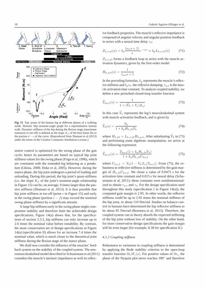
Fig. 15 Top: poses of the human leg in different phases of a walkingstride. Bottom: Hip moment-angle graph for a representative humanwalk. Dynamic stiffness of the hip during the flexion stage (maximumextension to toe-off) is defined as the slopeKf of the best linear fits tothe portiond− e of the curve. (Reproduced from Shamaei et al (2013)under the terms of the Creative Commons Attribution License.)
sistive control is optimized for the swing phase of the gaitcycle; hence its parameters are based on typical hip jointstiffness values for the swing phase (Frigo et al, 1996), whichare consistent with the extended leg behaving as a pendu-lum (Ghista, 2008; Doke et al, 2005). However, during thestance phase, the hip joint undergoes a period of loading andunloading. During this period, the hip joint’s quasi-stiffness(i.e. the slopeKf of the joint’s moment-angle relationshipin Figure 15) can be, on average, 9 times larger than the pas-sive stiffness (Shamaei et al, 2013). It is thus possible thathip joint stiffness at toe-off (pointe in Figure 15) and earlyin the swing phase (portione − f ) may exceed the nominalswing-phase stiffness by a significant amount.
A large hip stiffness early in the swing phase might com-promise stability and therefore limit the achievable designspecifications. Figure 14(a) shows that, for the specifica-tions of section 3.3.3, hip stiffness can only increase up to2.6 times the nominal value before instability. By contrast,the more conservative set of design specifications in Figure14(a) (specification II) allows for an increase 7.4 times thenominal value, which is much closer to the theoretical jointstiffness during the flexion stage of the stance phase.
We shall now consider the influence of the muscles’ feed-back system on the stability of the coupled system. The neu-romusculoskeletal model described in Schuurmans et al (2011)considers the muscle’s intrinsic impedance as well its reflex-
ive feedback properties. The muscle’s reflexive impedance iscomposed of angular velocity and angular position feedbackin series with a neural time delayτd:
Zh,refl(s) = kp(αvs+ 1)
se−τds ≡ kpLh,refl(s) (71)
Zh,refl forms a feedback loop in series with the muscle ac-tivation dynamics, given by the first-order model
Hh,act(s) =1
τacts+ 1(72)
In the preceding formulas,kp represents the muscle’s reflex-ive stiffness andkpαv the reflexive damping;τact is the mus-cle activation time constant. To analyze coupled stability, wedefine a new perturbed closed-loop transfer function
Thecf(s) =1
1 + (Yh + Yc)Zef
(73)
In this caseYh represents the leg’s musculoskeletal systemwith muscle activation feedback, and is given by
Yh(s) =Yh
1 + kpHh,fbYh
(74)
whereHh,fb = Lh,reflHh,act. After substitutingYh in (73)and performing some algebraic manipulation, we arrive atthe following expression
Thecf(s) =Thecf (1 + kpHh,fbYh)
1 + kpHh,fbUhecf
(75)
whereUhecf = Yh(1 − YhZefThecf). From (75), the ro-bustness to reflexive stiffness is determined by the gain mar-gin of Hh,fbUhecf . We chose a value of 0.0475 s for theactivation time constant and 0.015 s for neural delay (Schu-urmans et al, 2011); these constants were nondimensional-ized to obtainτact andτd. For the design specification usedthroughout this study (specification I in Figure 14(a)), thecomputed gain margin is 2.95. In other words, the reflexivestiffness could be up to 2.95 times the nominal stiffness ofthe hip joint, or about 110 Nm/rad. Studies on balance con-trol in humans have determined the hip reflexive stiffness tobe about 95 Nm/rad (Boonstra et al, 2013). Therefore, thecoupled system can in theory absorb the expected stiffeningof the hip joint without loss of stability. On the other hand,for more conservative design specifications the gain marginwill be even larger (for example, 8.38 for specification II.)
4.1.2 Coupling stiffness
Robustness to variations in coupling stiffness is determinedby applying the Bode stability criterion to the open-looptransfer functionδkcWc(s). For positive values ofδkc, thephase of the Nyquist plot never reaches 180 and therefore

An admittance shaping controller for exoskeleton assistance of the lower extremities 19
the variation margin forδkc is infinite, whereas for nega-tive δkc there is the margin is finite (Figure 14(b)). This isconsistent with what we see in Figure 10: overall, to lowervalues of coupling stiffnessωn,ec correspond lower stabilitymargins. Therefore, like in the case of hip joint stiffness,fordesign purposes it is safer to underestimate the stiffness ofthe coupling.
4.2 Robustness to exoskeleton damping
Ideally, the inner-loop control should make the exoskele-ton arm behave as a pure inertia (section 3.2). However, wewant to consider the case in which that behavior is not pro-duced with complete accuracy. A specific question is, if theinner-loop control generates a certain amount of negativedamping instead of dead-on zero damping, will that destabi-lize the coupled human-exoskeleton system? For one thing,we know that, when assistance is on (Ic > 0), there is al-ready negative damping present, as the exoskeleton’s portimpedance has a negative real part. Yet the coupled systemremains theoretically stable. The question is then whetherunintended negative damping from the inner-loop controlmight, in a sense, push the system over the limit and make itunstable.
To answer that question, we generate another perturbedversion ofThecf by substitutingZef in (62) with Zef =
Zef+δbe, whereδbe is the variation from the ideal zero exo-skeleton damping. It can be shown that the resulting transferfunctionThecf has a characteristic equation
1 + δbeWe(s) = 0 (76)
where
We(s) =1− Thecf
Zef
(77)
Figure 14(c) shows the Nyquist plot ofδbeWe(s) for theextremal negative variationδbe,min. Clearly, there is a con-siderable stability margin for negative exoskeleton damping;the magnitude ofδbe could in theory be about 70% the hu-man dampingbh without loss of stability. On the other hand,there is an infinite stability margin for positive values ofδbe.In other words, positive exoskeleton damping would only in-crease the stability of the coupled system, albeit at the costof reduced performance due to additional energy dissipation.
4.3 Robustness to time delay in the exoskeleton control andother nonlinearities
Time delays in the exoskeleton control, such as are intro-duced by sensing and estimation, can be additional sources
Fig. 16 Dynamic walker (DW) model. The DW’s gait undergoes twophases: (a) leg swing with knee joint passively flexing and (2) leg swingwith knee joint locked.
of instability. This, in turn, may require verifying the con-trol’s phase margins. For example, in the SMA device (Fig-ure 1(a)), the angular position of the motor’s output shaft ismeasured by an array of Hall effect sensors with a resolu-tion (gearing considered) of 600 counts per revolution. Inorder to eliminate quantization noise, angular velocity andacceleration of the shaft are estimated using a model-freeKalman filter (Belanger et al, 1998). For a 1.0 Hz sinusoidalmotion, the delay in the acceleration estimate is between 4and 5 time steps, or about 16 phase.
Figure 12(c) shows that, for the feedback compensatorexample in section 3.4.2, the phase margin is infinite; inother words, a pure phase delay cannot cause instability.However, for a more demanding design specification thismay not be the case. In such a situation, a possible strat-egy can be to include a linearized model of the accelerationestimator in the feedback compensator model (50), i.e. makethe estimator part of the control design.
On the other hand, nonlinearities such as backlash or ac-tuator could give rise to limit cycles. In the SMA itself, mo-tor torque is delivered through a custom-designed harmonicdrive with a gearing ratio of 10:1. The drive as such is vir-tually backlash-free and therefore less likely to cause limitcycling than a conventional gear transmission. However, iflimit cycles do arise they can be counteracted by the inner-loop control (section 3.2), for example through the use of alead compensator.
5 Assisting human gait: bipedal walk simulations andinitial trials with the exoskeleton
The use of our assistive control for actual walking will be theobject of a separate study. Here we offer a few initial consid-erations on assisting bipedal gait. We simulated the assistivecontrol on a previously published dynamical bipedal walk-ing model (Aguirre-Ollinger, 2014). The dynamic walker
20 Gabriel Aguirre-Ollinger et al.
−^_`
−0.2
0
0.2
^_`
(b) θ1(t), rad
Θss
= 0.345 rad
0.4
0.6
0.8
1
1.2
(a) fstep
(t), Hz
fstep, ss
= 0.905 Hz fstep, ss
= 1.061 Hz
0 10 20 300
0.2
0.4
0.6
t (s)
(c) v(t), m/sv
ss= 0.507 m/s
0 10 20 30t (s)
vss
= 0.621 m/s
Θss
= 0.358 rad
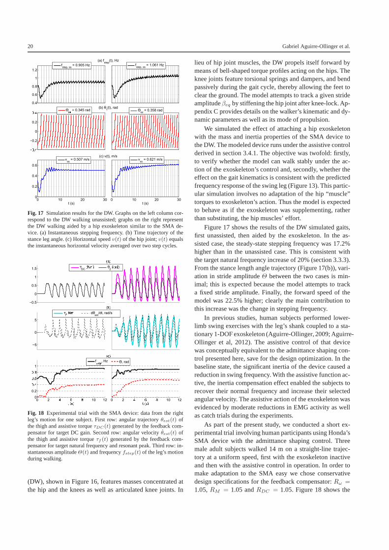
Fig. 17 Simulation results for the DW. Graphs on the left column cor-respond to the DW walking unassisted; graphs on the right representthe DW walking aided by a hip exoskeleton similar to the SMA de-vice. (a) Instantaneous stepping frequency. (b) Time trajectory of thestance leg angle. (c) Horizontal speedv(t) of the hip joint;v(t) equalsthe instantaneous horizontal velocity averaged over two step cycles.
−0.5
0
0.5
1
1.5
ehj
−5
0
5
ekj
0 2 l m n 10 120
0.2
pql
pqm
pqn
1
r evj
ewj
τDC
exyj θ2ezhj
0 2 l m n 10 12
r evj
f|~
, Hz Θ, rad
τf xy dθ
est/dt, rad/s
Fig. 18 Experimental trial with the SMA device: data from the rightleg’s motion for one subject. First row: angular trajectoryθest(t) ofthe thigh and assistive torqueτDC(t) generated by the feedback com-pensator for target DC gain. Second row: angular velocityθest(t) ofthe thigh and assistive torqueτf (t) generated by the feedback com-pensator for target natural frequency and resonant peak. Third row: in-stantaneous amplitudeΘ(t) and frequencyfstep(t) of the leg’s motionduring walking.
(DW), shown in Figure 16, features masses concentrated atthe hip and the knees as well as articulated knee joints. In
lieu of hip joint muscles, the DW propels itself forward bymeans of bell-shaped torque profiles acting on the hips. Theknee joints feature torsional springs and dampers, and bendpassively during the gait cycle, thereby allowing the feet toclear the ground. The model attempts to track a given strideamplitudeβeq by stiffening the hip joint after knee-lock. Ap-pendix C provides details on the walker’s kinematic and dy-namic parameters as well as its mode of propulsion.
We simulated the effect of attaching a hip exoskeletonwith the mass and inertia properties of the SMA device tothe DW. The modeled device runs under the assistive controlderived in section 3.4.1. The objective was twofold: firstly,to verify whether the model can walk stably under the ac-tion of the exoskeleton’s control and, secondly, whether theeffect on the gait kinematics is consistent with the predictedfrequency response of the swing leg (Figure 13). This partic-ular simulation involves no adaptation of the hip “muscle”torques to exoskeleton’s action. Thus the model is expectedto behave as if the exoskeleton was supplementing, ratherthan substituting, the hip muscles’ effort.
Figure 17 shows the results of the DW simulated gaits,first unassisted, then aided by the exoskeleton. In the as-sisted case, the steady-state stepping frequency was 17.2%higher than in the unassisted case. This is consistent withthe target natural frequency increase of 20% (section 3.3.3).From the stance length angle trajectory (Figure 17(b)), vari-ation in stride amplitudeΘ between the two cases is min-imal; this is expected because the model attempts to tracka fixed stride amplitude. Finally, the forward speed of themodel was 22.5% higher; clearly the main contribution tothis increase was the change in stepping frequency.
In previous studies, human subjects performed lower-limb swing exercises with the leg’s shank coupled to a sta-tionary 1-DOF exoskeleton (Aguirre-Ollinger, 2009; Aguirre-Ollinger et al, 2012). The assistive control of that devicewas conceptually equivalent to the admittance shaping con-trol presented here, save for the design optimization. In thebaseline state, the significant inertia of the device causedareduction in swing frequency. With the assistive function ac-tive, the inertia compensation effect enabled the subjectstorecover their normal frequency and increase their selectedangular velocity. The assistive action of the exoskeleton wasevidenced by moderate reductions in EMG activity as wellas catch trials during the experiments.
As part of the present study, we conducted a short ex-perimental trial involving human participants using Honda’sSMA device with the admitttance shaping control. Threemale adult subjects walked 14 m on a straight-line trajec-tory at a uniform speed, first with the exoskeleton inactiveand then with the assistive control in operation. In order tomake adaptation to the SMA easy we chose conservativedesign specifications for the feedback compensator:Rω =
1.05,RM = 1.05 andRDC = 1.05. Figure 18 shows the
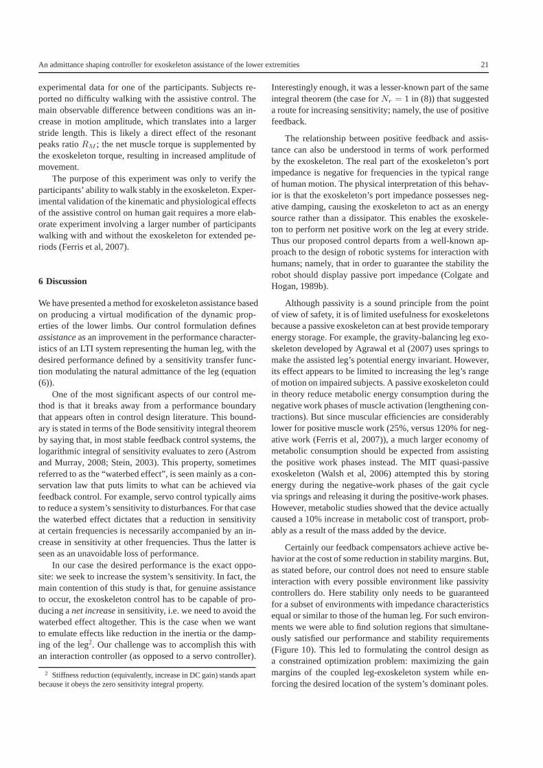
An admittance shaping controller for exoskeleton assistance of the lower extremities 21
experimental data for one of the participants. Subjects re-ported no difficulty walking with the assistive control. Themain observable difference between conditions was an in-crease in motion amplitude, which translates into a largerstride length. This is likely a direct effect of the resonantpeaks ratioRM ; the net muscle torque is supplemented bythe exoskeleton torque, resulting in increased amplitude ofmovement.
The purpose of this experiment was only to verify theparticipants’ ability to walk stably in the exoskeleton. Exper-imental validation of the kinematic and physiological effectsof the assistive control on human gait requires a more elab-orate experiment involving a larger number of participantswalking with and without the exoskeleton for extended pe-riods (Ferris et al, 2007).
6 Discussion
We have presented a method for exoskeleton assistance basedon producing a virtual modification of the dynamic prop-erties of the lower limbs. Our control formulation definesassistanceas an improvement in the performance character-istics of an LTI system representing the human leg, with thedesired performance defined by a sensitivity transfer func-tion modulating the natural admittance of the leg (equation(6)).
One of the most significant aspects of our control me-thod is that it breaks away from a performance boundarythat appears often in control design literature. This bound-ary is stated in terms of the Bode sensitivity integral theoremby saying that, in most stable feedback control systems, thelogarithmic integral of sensitivity evaluates to zero (Astromand Murray, 2008; Stein, 2003). This property, sometimesreferred to as the “waterbed effect”, is seen mainly as a con-servation law that puts limits to what can be achieved viafeedback control. For example, servo control typically aimsto reduce a system’s sensitivity to disturbances. For that casethe waterbed effect dictates that a reduction in sensitivityat certain frequencies is necessarily accompanied by an in-crease in sensitivity at other frequencies. Thus the latterisseen as an unavoidable loss of performance.
In our case the desired performance is the exact oppo-site: we seek to increase the system’s sensitivity. In fact,themain contention of this study is that, for genuine assistanceto occur, the exoskeleton control has to be capable of pro-ducing anet increasein sensitivity, i.e. we need to avoid thewaterbed effect altogether. This is the case when we wantto emulate effects like reduction in the inertia or the damp-ing of the leg2. Our challenge was to accomplish this withan interaction controller (as opposed to a servo controller).
2 Stiffness reduction (equivalently, increase in DC gain) stands apartbecause it obeys the zero sensitivity integral property.
Interestingly enough, it was a lesser-known part of the sameintegral theorem (the case forNr = 1 in (8)) that suggesteda route for increasing sensitivity; namely, the use of positivefeedback.
The relationship between positive feedback and assis-tance can also be understood in terms of work performedby the exoskeleton. The real part of the exoskeleton’s portimpedance is negative for frequencies in the typical rangeof human motion. The physical interpretation of this behav-ior is that the exoskeleton’s port impedance possesses neg-ative damping, causing the exoskeleton to act as an energysource rather than a dissipator. This enables the exoskele-ton to perform net positive work on the leg at every stride.Thus our proposed control departs from a well-known ap-proach to the design of robotic systems for interaction withhumans; namely, that in order to guarantee the stability therobot should display passive port impedance (Colgate andHogan, 1989b).
Although passivity is a sound principle from the pointof view of safety, it is of limited usefulness for exoskeletonsbecause a passive exoskeleton can at best provide temporaryenergy storage. For example, the gravity-balancing leg exo-skeleton developed by Agrawal et al (2007) uses springs tomake the assisted leg’s potential energy invariant. However,its effect appears to be limited to increasing the leg’s rangeof motion on impaired subjects. A passive exoskeleton couldin theory reduce metabolic energy consumption during thenegative work phases of muscle activation (lengthening con-tractions). But since muscular efficiencies are considerablylower for positive muscle work (25%, versus 120% for neg-ative work (Ferris et al, 2007)), a much larger economy ofmetabolic consumption should be expected from assistingthe positive work phases instead. The MIT quasi-passiveexoskeleton (Walsh et al, 2006) attempted this by storingenergy during the negative-work phases of the gait cyclevia springs and releasing it during the positive-work phases.However, metabolic studies showed that the device actuallycaused a 10% increase in metabolic cost of transport, prob-ably as a result of the mass added by the device.
Certainly our feedback compensators achieve active be-havior at the cost of some reduction in stability margins. But,as stated before, our control does not need to ensure stableinteraction with every possible environment like passivitycontrollers do. Here stability only needs to be guaranteedfor a subset of environments with impedance characteristicsequal or similar to those of the human leg. For such environ-ments we were able to find solution regions that simultane-ously satisfied our performance and stability requirements(Figure 10). This led to formulating the control design asa constrained optimization problem: maximizing the gainmargins of the coupled leg-exoskeleton system while en-forcing the desired location of the system’s dominant poles.
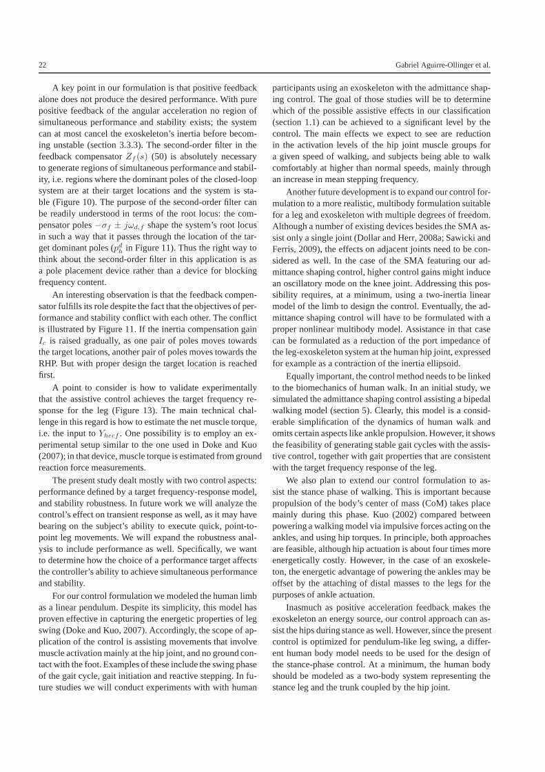
22 Gabriel Aguirre-Ollinger et al.
A key point in our formulation is that positive feedbackalone does not produce the desired performance. With purepositive feedback of the angular acceleration no region ofsimultaneous performance and stability exists; the systemcan at most cancel the exoskeleton’s inertia before becom-ing unstable (section 3.3.3). The second-order filter in thefeedback compensatorZf (s) (50) is absolutely necessaryto generate regions of simultaneous performance and stabil-ity, i.e. regions where the dominant poles of the closed-loopsystem are at their target locations and the system is sta-ble (Figure 10). The purpose of the second-order filter canbe readily understood in terms of the root locus: the com-pensator poles−σf ± jωd,f shape the system’s root locusin such a way that it passes through the location of the tar-get dominant poles (pdh in Figure 11). Thus the right way tothink about the second-order filter in this application is asa pole placement device rather than a device for blockingfrequency content.
An interesting observation is that the feedback compen-sator fulfills its role despite the fact that the objectives of per-formance and stability conflict with each other. The conflictis illustrated by Figure 11. If the inertia compensation gainIc is raised gradually, as one pair of poles moves towardsthe target locations, another pair of poles moves towards theRHP. But with proper design the target location is reachedfirst.
A point to consider is how to validate experimentallythat the assistive control achieves the target frequency re-sponse for the leg (Figure 13). The main technical chal-lenge in this regard is how to estimate the net muscle torque,i.e. the input toYhecf . One possibility is to employ an ex-perimental setup similar to the one used in Doke and Kuo(2007); in that device, muscle torque is estimated from groundreaction force measurements.
The present study dealt mostly with two control aspects:performance defined by a target frequency-response model,and stability robustness. In future work we will analyze thecontrol’s effect on transient response as well, as it may havebearing on the subject’s ability to execute quick, point-to-point leg movements. We will expand the robustness anal-ysis to include performance as well. Specifically, we wantto determine how the choice of a performance target affectsthe controller’s ability to achieve simultaneous performanceand stability.
For our control formulation we modeled the human limbas a linear pendulum. Despite its simplicity, this model hasproven effective in capturing the energetic properties of legswing (Doke and Kuo, 2007). Accordingly, the scope of ap-plication of the control is assisting movements that involvemuscle activation mainly at the hip joint, and no ground con-tact with the foot. Examples of these include the swing phaseof the gait cycle, gait initiation and reactive stepping. Infu-ture studies we will conduct experiments with with human
participants using an exoskeleton with the admittance shap-ing control. The goal of those studies will be to determinewhich of the possible assistive effects in our classification(section 1.1) can be achieved to a significant level by thecontrol. The main effects we expect to see are reductionin the activation levels of the hip joint muscle groups fora given speed of walking, and subjects being able to walkcomfortably at higher than normal speeds, mainly throughan increase in mean stepping frequency.
Another future development is to expand our control for-mulation to a more realistic, multibody formulation suitablefor a leg and exoskeleton with multiple degrees of freedom.Although a number of existing devices besides the SMA as-sist only a single joint (Dollar and Herr, 2008a; Sawicki andFerris, 2009), the effects on adjacent joints need to be con-sidered as well. In the case of the SMA featuring our ad-mittance shaping control, higher control gains might inducean oscillatory mode on the knee joint. Addressing this pos-sibility requires, at a minimum, using a two-inertia linearmodel of the limb to design the control. Eventually, the ad-mittance shaping control will have to be formulated with aproper nonlinear multibody model. Assistance in that casecan be formulated as a reduction of the port impedance ofthe leg-exoskeleton system at the human hip joint, expressedfor example as a contraction of the inertia ellipsoid.
Equally important, the control method needs to be linkedto the biomechanics of human walk. In an initial study, wesimulated the admittance shaping control assisting a bipedalwalking model (section 5). Clearly, this model is a consid-erable simplification of the dynamics of human walk andomits certain aspects like ankle propulsion. However, it showsthe feasibility of generating stable gait cycles with the assis-tive control, together with gait properties that are consistentwith the target frequency response of the leg.
We also plan to extend our control formulation to as-sist the stance phase of walking. This is important becausepropulsion of the body’s center of mass (CoM) takes placemainly during this phase. Kuo (2002) compared betweenpowering a walking model via impulsive forces acting on theankles, and using hip torques. In principle, both approachesare feasible, although hip actuation is about four times moreenergetically costly. However, in the case of an exoskele-ton, the energetic advantage of powering the ankles may beoffset by the attaching of distal masses to the legs for thepurposes of ankle actuation.
Inasmuch as positive acceleration feedback makes theexoskeleton an energy source, our control approach can as-sist the hips during stance as well. However, since the presentcontrol is optimized for pendulum-like leg swing, a differ-ent human body model needs to be used for the design ofthe stance-phase control. At a minimum, the human bodyshould be modeled as a two-body system representing thestance leg and the trunk coupled by the hip joint.

An admittance shaping controller for exoskeleton assistance of the lower extremities 23
References
Agrawal S, Banala S, Fattah A, Sangwan V, Krishnamoor-thy V, Scholz J, Wei-Li H (2007) Assessment of motionof a swing leg and gait rehabilitation with a gravity bal-ancing exoskeleton. Neural Systems and RehabilitationEngineering, IEEE Transactions on 15(3):410–420, DOI10.1109/TNSRE.2007.903930
Aguirre-Ollinger G (2009) Active impedance control of alower-limb assistive exoskeleton. dissertation, Northwest-ern University, Evanston, IL
Aguirre-Ollinger G (2013) Learning muscle activation pat-terns via nonlinear oscillators: Application to lower-limbassistance. In: Intelligent Robots and Systems (IROS),2013 IEEE/RSJ International Conference on, pp 1182–1189
Aguirre-Ollinger G (2014) Globally stable control of a dy-namic bipedal walker using adaptive frequency oscilla-tors. Robotica 32(7):1039–1063
Aguirre-Ollinger G (2015) Exoskeleton control for lower-extremity assistance based on adaptive frequency oscil-lators: Adaptation of muscle activation and movementfrequency. Proceedings of the Institution of MechanicalEngineers, Part H: Journal of Engineering in Medicine229(1):52–68, DOI 10.1177/0954411914567213
Aguirre-Ollinger G, Colgate J, Peshkin M, Goswami A(2007) A 1-DOF assistive exoskeleton with virtual nega-tive damping: effects on the kinematic response of the lo-wer limbs. In: IEEE/RSJ International Conference on In-telligent Robots and Systems IROS 2007, pp 1938–1944
Aguirre-Ollinger G, Colgate J, Peshkin M, Goswami A(2011) Design of an active one-degree-of-freedom lower-limb exoskeleton with inertia compensation. The Interna-tional Journal of Robotics Research 30(4):486–499
Aguirre-Ollinger G, Colgate J, Peshkin M, Goswami A(2012) Inertia compensation control of a one-degree-of-freedom exoskeleton for lower-limb assistance: Initial ex-periments. Neural Systems and Rehabilitation Engineer-ing, IEEE Transactions on 20(1):68–77
American Honda Motor Co, Inc (2009) Honda- walk assist and mobility devices. URLcorporate.honda.com/innovation/walk-assist
Astrom KJ, Murray RM (2008) Feedback Systems: An In-troduction for Scientists and Engineers. Princeton Univer-sity Press, Princeton, NJ, USA
Banala S, Agrawal SK, Fattah A, Krishnamoorthy V, HsuWL, Scholz J, Rudolph K (2006) Gravity-balancing legorthosis and its performance evaluation. IEEE Transac-tions on Robotics 22(6):1228–1239
Banala S, Kim S, Agrawal S, Scholz J (2009) Robot assistedgait training with active leg exoskeleton (ALEX). NeuralSystems and Rehabilitation Engineering, IEEE Transac-tions on 17(1):2–8
Belanger P, Dobrovolny P, Helmy A, Zhang X (1998)Estimation of angular velocity and acceleration fromshaft-encoder measurements. The International Journal ofRobotics Research 17(11):1225–1233
Bernhardt M, Frey M, Colombo G, Riener R (2005) Hybridforce-position control yields cooperative behaviour ofthe rehabilitation robot lokomat. Rehabilitation Robotics,2005 ICORR 2005 9th International Conference on pp536–539
Blaya J, Herr H (2004) Adaptive control of a variable-impedance ankle-foot orthosis to assist drop-foot gait.Neural Systems and Rehabilitation Engineering, IEEETransactions on 12(1):24–31
Boonstra T, Schouten A, van der Kooij H (2013) Identifi-cation of the contribution of the ankle and hip joints tomulti-segmental balance control. Journal of NeuroEngi-neering and Rehabilitation 10(23):1–18
Buerger S, Hogan N (2007) Complementary stability andloop shaping for improved human-robot interaction.Robotics, IEEE Transactions on 23(2):232–244
Colgate E, Hogan N (1989a) The interaction of robotswith passive environments: Application to force feedbackcontrol. Fourth International Conference on AdvancedRobotics
Colgate J, Hogan N (1988) Robust control of dynami-cally interacting systems. International Journal of Control48(1):65–88
Colgate J, Hogan N (1989b) An analysis of contact insta-bility in terms of passive physical equivalents. Proceed-ings of the IEEE International Conference on Roboticsand Automation pp 404–409
Doke J, Kuo AD (2007) Energetic cost of producing cyclicmuscle force, rather than work, to swing the human leg.Journal of Experimental Biology 210:2390–2398
Doke J, Donelan JM, Kuo AD (2005) Mechanics and ener-getics of swinging the human leg. Journal of Experimen-tal Biology 208:439–445
Dollar A, Herr H (2008a) Design of a quasi-passive kneeexoskeleton to assist running. 2008 IEEE/RSJ Interna-tional Conference on Intelligent Robots and Systems pp747–754
Dollar A, Herr H (2008b) Lower extremity exoskeletonsand active orthoses: Challenges and state of the art. IEEETransactions on Robotics 24(1):144–158
Ekso BionicsTM (2013) Ekso bionics - an exoskeleton bionicsuit or a wearable robot that helps people walk again.URL www.eksobionics.com
Emken J, Wynne J, Harkema S, Reinkensmeyer D (2006)A robotic device for manipulating human stepping.Robotics, IEEE Transactions on 22(1):185–189
European Commission (CORDIS) (2013) Balance Augmen-tation in Locomotion, through Anticipative, Natural andCooperative control of Exoskeletons (BALANCE). URL
24 Gabriel Aguirre-Ollinger et al.
cordis.europa.eu/projects/rcn/106854_en.html
Fee J, Miller F (2004) The leg drop pendulum test performedunder general anesthesia in spastic cerebral palsy. Devel-opmental Medicine and Child Neurology 46:273–281
Ferris D, Sawicki G, Daley M (2007) A physiologist’s per-spective on robotic exoskeletons for human locomotion.International Journal of Humanoid Robotics 4:507–528
Frigo C, Crenna P, Jensen L (1996) Moment-angle relation-ship at lower limb joints during human walking at differ-ent velocities. Journal of Electromyography and Kinesi-ology 6(3):177–190
Ghista D (2008) Applied Biomedical Engineering Mechan-ics. CRC Press
Gordon K, Kinnaird C, Ferris D (2013) Locomotor adapta-tion to a soleus EMG-controlled antagonistic exoskeleton.Journal of Neurophysiology 109(7):1804–1814
Hogan N, Buerger S (2006) Relaxing passivity for human-robot interaction. Proceedings of the 2006 IEEE/RSJ In-ternational Conference on Intelligent Robots and Systems
Hogan N, Krebs HI, Rohrer B, Palazzolo J, Dipietro L, Fa-soli S, Stein J, Hughes R, Frontera W, Lynch D, Volpe B(2006) Motions or muscles? some behavioral factors un-derlying robotic assistance of motor recovery. Journal ofrehabilitation research and development 43(5):605
Kawamoto H, Sankai Y (2005) Power assist method basedon phase sequence and muscle force condition for HAL.Advanced Robotics 19(7):717–734
Kawamoto H, Lee S, Kanbe S, Sankai Y (2003) Power assistmethod for HAL-3 using EMG-based feedback controller.In: Systems, Man and Cybernetics, 2003. IEEE Interna-tional Conference on, vol 2, pp 1648–1653 vol.2
Kazerooni H, Racine J, Huang R Land Steger (2005) Onthe control of the berkeley lower extremity exoskele-ton (BLEEX). In: Proceedings of the IEEE InternationalConference on Robotics and Automation ICRA 2005, pp4353–4360
Kuo AD (2002) Energetics of actively powered locomotionusing the simplest walking model. Journal of Biomechan-ical Engineering 124:113–120
Lee S, Sankai Y (2003) The natural frequency-based powerassist control for lower body with HAL-3. IEEE Inter-national Conference on Systems, Man and Cybernetics2:1642–1647
Lenzi T, Carrozza M, Agrawal S (2013) Powered hip ex-oskeletons can reduce the user’s hip and ankle muscle ac-tivations during walking. Neural Systems and Rehabilita-tion Engineering, IEEE Transactions on 21(6):938–948
Lewis C, Ferris D (2011) Invariant hip moment pattern whilewalking with a robotic hip exoskeleton. Journal of Biome-chanics 44(5):789–793
Malcolm P, Derave W, Galle S, De Clercq D (2013) Asimple exoskeleton that assists plantarflexion can re-duce the metabolic cost of human walking. PLoS ONE
8(2):e56,137, DOI 10.1371/journal.pone.0056137Middleton R, Braslavsky J (2000) On the relationship be-
tween logarithmic sensitivity integrals and limiting opti-mal control problems. Decision and Control, 2000 Pro-ceedings of the 39th IEEE Conference on 5:4990–4995vol.5
Mooney L, Rouse E, Herr H (2014) Autonomous exoskele-ton reduces metabolic cost of human walking during loadcarriage. Journal of NeuroEngineering and Rehabilitation11(1):80
More J, Sorensen D (1983) Computing a trust region step.SIAM Journal on Scientific and Statistical Computing4(3):553–572
Nef T, Mihelj M, Riener R (2007) ARMin: a robot forpatient-cooperative arm therapy. Medical & BiologicalEngineering & Computing 45(9):887–900
Norris J, Granata KP, Mitros MR, Byrne EM, Marsh AP(2007) Effect of augmented plantarflexion power on pre-ferred walking speed and economy in young and olderadults. Gait & Posture 25:620–627
Petric T, Gams A, Ijspeert A, Zlajpah L (2011) On-line fre-quency adaptation and movement imitation for rhythmicrobotic tasks. International Journal of Robotics Research30(14):1775–1788
Ronsse R, Lenzi T, Vitiello N, Koopman B, van AsseldonkE, De Rossi SM, van den Kieboom J, van der Kooij H,Carrozza M, Ijspeert A (2011) Oscillator-based assistanceof cyclical movements: model-based and model-free ap-proaches. Medical & Biological Engineering & Comput-ing 49(10):1173–1185
Royer TD, Martin PE (2005) Manipulations of leg massand moment of inertia: Effects on energy cost of walking.Medicine and Science in Sports and Exercise 37(4):649–656
Sawicki G, Ferris D (2008) Mechanics and energetics oflevel walking with powered ankle exoskeletons. Journalof Experimental Biology 211:1402–1413
Sawicki G, Ferris D (2009) Powered ankle exoskeletons re-veal the metabolic cost of plantar flexor mechanical workduring walking with longer steps at constant step fre-quency. Journal of Experimental Biology 212:21–31
Schouten A, Vlugt E, Van der Helm F (2008) Design ofperturbation signals for the estimation of proprioceptivereflexes. IEEE Transactions on Biomedical Engineering55(5):1612–1619
Schuurmans J, van der Helm F, Schouten A (2011) Re-lating reflex gain modulation in posture control to un-derlying neural network properties using a neuromuscu-loskeletal model. Journal of Computational Neuroscience30(3):555–565
Shamaei K, Sawicki G, Dollar A (2013) Estimation of quasi-stiffness of the human hip in the stance phase of walking.PLoS ONE 8(12):e81,841, DOI 10.1371/journal.pone.
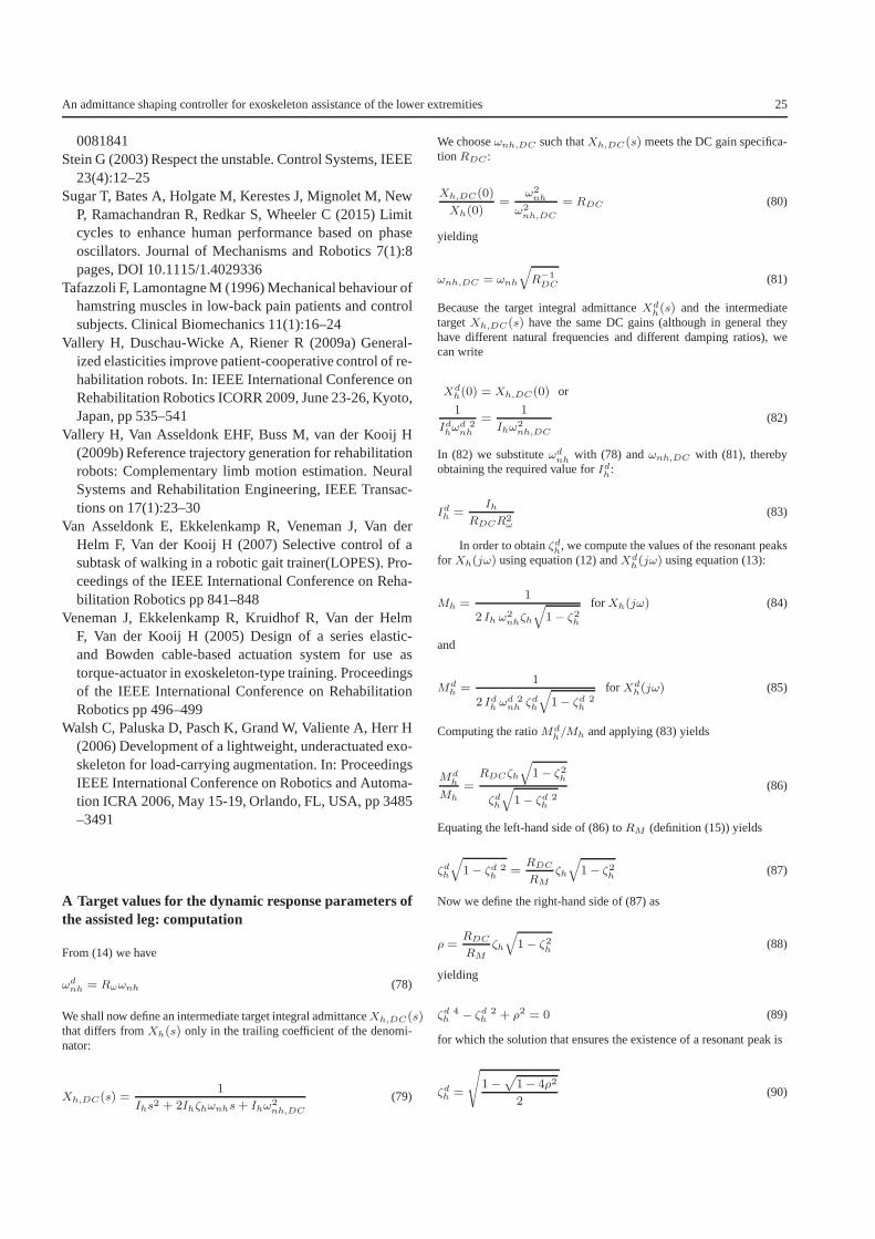
An admittance shaping controller for exoskeleton assistance of the lower extremities 25
0081841Stein G (2003) Respect the unstable. Control Systems, IEEE
23(4):12–25Sugar T, Bates A, Holgate M, Kerestes J, Mignolet M, New
P, Ramachandran R, Redkar S, Wheeler C (2015) Limitcycles to enhance human performance based on phaseoscillators. Journal of Mechanisms and Robotics 7(1):8pages, DOI 10.1115/1.4029336
Tafazzoli F, Lamontagne M (1996) Mechanical behaviour ofhamstring muscles in low-back pain patients and controlsubjects. Clinical Biomechanics 11(1):16–24
Vallery H, Duschau-Wicke A, Riener R (2009a) General-ized elasticities improve patient-cooperative control ofre-habilitation robots. In: IEEE International Conference onRehabilitation Robotics ICORR 2009, June 23-26, Kyoto,Japan, pp 535–541
Vallery H, Van Asseldonk EHF, Buss M, van der Kooij H(2009b) Reference trajectory generation for rehabilitationrobots: Complementary limb motion estimation. NeuralSystems and Rehabilitation Engineering, IEEE Transac-tions on 17(1):23–30
Van Asseldonk E, Ekkelenkamp R, Veneman J, Van derHelm F, Van der Kooij H (2007) Selective control of asubtask of walking in a robotic gait trainer(LOPES). Pro-ceedings of the IEEE International Conference on Reha-bilitation Robotics pp 841–848
Veneman J, Ekkelenkamp R, Kruidhof R, Van der HelmF, Van der Kooij H (2005) Design of a series elastic-and Bowden cable-based actuation system for use astorque-actuator in exoskeleton-type training. Proceedingsof the IEEE International Conference on RehabilitationRobotics pp 496–499
Walsh C, Paluska D, Pasch K, Grand W, Valiente A, Herr H(2006) Development of a lightweight, underactuated exo-skeleton for load-carrying augmentation. In: ProceedingsIEEE International Conference on Robotics and Automa-tion ICRA 2006, May 15-19, Orlando, FL, USA, pp 3485–3491
A Target values for the dynamic response parameters ofthe assisted leg: computation
From (14) we have
ωdnh = Rωωnh (78)
We shall now define an intermediate target integral admittanceXh,DC(s)that differs fromXh(s) only in the trailing coefficient of the denomi-nator:
Xh,DC(s) =1
Ihs2 + 2Ihζhωnhs+ Ihω2
nh,DC
(79)
We chooseωnh,DC such thatXh,DC(s) meets the DC gain specifica-tionRDC :
Xh,DC(0)
Xh(0)=
ω2
nh
ω2
nh,DC
= RDC (80)
yielding
ωnh,DC = ωnh
√
R−1
DC(81)
Because the target integral admittanceXdh(s) and the intermediate
targetXh,DC(s) have the same DC gains (although in general theyhave different natural frequencies and different damping ratios), wecan write
Xdh(0) = Xh,DC(0) or
1
Idhωd 2
nh
=1
Ihω2
nh,DC
(82)
In (82) we substituteωdnh
with (78) andωnh,DC with (81), therebyobtaining the required value forId
h:
Idh =Ih
RDCR2ω
(83)
In order to obtainζdh
, we compute the values of the resonant peaksfor Xh(jω) using equation (12) andXd
h(jω) using equation (13):
Mh =1
2 Ih ω2
nhζh
√
1 − ζ2h
for Xh(jω) (84)
and
Mdh =
1
2 Idhωd 2
nhζdh
√
1− ζd 2
h
for Xdh(jω) (85)
Computing the ratioMdh/Mh and applying (83) yields
Mdh
Mh
=RDCζh
√
1− ζ2h
ζdh
√
1− ζd 2
h
(86)
Equating the left-hand side of (86) toRM (definition (15)) yields
ζdh
√
1− ζd 2
h=RDC
RM
ζh
√
1− ζ2h
(87)
Now we define the right-hand side of (87) as
ρ =RDC
RM
ζh
√
1− ζ2h
(88)
yielding
ζd 4
h − ζd 2
h + ρ2 = 0 (89)
for which the solution that ensures the existence of a resonant peak is
ζdh =
√
1 −√
1− 4ρ2
2(90)
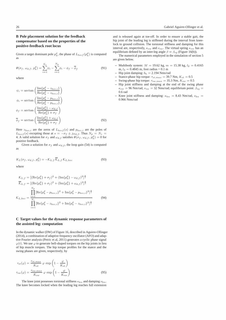
26 Gabriel Aguirre-Ollinger et al.
B Pole placement solution for the feedbackcompensator based on the properties of thepositive-feedback root locus
Given a target dominant polepdh
, the phase ofLhecf (pdh) is computed
as
Φ(σf , ωd,f , pdh) =
Nz∑
i=1
ψi −
Np∑
i=1
φi − φf − φf (91)
where
ψi = arctan
(
Impdh− zhec,i
Repdh− zhec,i
)
φi = arctan
(
Impdh− phec,i
Repdh− phec,i
)
φf = arctan
(
Impdh − ωd,f
Repdh+ σf
)
φf = arctan
(
Impdh+ ωd,f
Repdh+ σf
)
(92)
Here zhec,i are the zeros ofLhecf (s) and phec,i are the poles ofLhecf (s) excepting those ats = −σf ± jωd,f . ThusNp = Nz =4. A valid solution forσf andωd,f satisfiesΦ(σf , ωd,f , p
dh) = 0 for
positive feedback.Given a solution forσf andωd,f , the loop gain (54) is computed
as
KL(σf , ωd,f , pdh) = −KL,f KL,f KL,hec (93)
where
KL,f = [(Repdh+ σf )2 + (Impdh − ωd,f )
2]1
2
KL,f = [(Repdh+ σf )2 + (Impdh+ ωd,f )
2]1
2
KL,hec =
Np∏
i=1
[Repdh − phec,i2 + Impdh − phec,i
2]1
2
Nz∏
i=1
[Repdh − zhec,i2 + Impdh − zhec,i
2]1
2
(94)
C Target values for the dynamic response parameters ofthe assisted leg: computation
In the dynamic walker (DW) of Figure 16, described in Aguirre-Ollinger(2014), a combination of adaptive frequency oscillator (AFO) and adap-tive Fourier analysis (Petric et al, 2011) generates a cyclic phase signalϕ(t). We useϕ to generate bell-shaped torques on the hip joints in lieuof hip muscle torques. The hip torque profiles for the stance and theswing phases are given, respectively, by
τst(ϕ) =τst,max
Kst
ϕ exp
(
1−ϕ
Kst
)
τsw(ϕ) =τsw,max
Ksw
ϕ exp
(
1−ϕ
Ksw
)
(95)
The knee joint possesses torsional stiffnessκkn and dampingνkn.The knee becomes locked when the leading leg reaches full extension
and is released again at toe-off. In order to ensure a stable gait, thehip joint of the leading leg is stiffened during the intervalfrom knee-lock to ground collision. The torsional stiffness and damping for thisinterval are, respectively,κsw andνsw. The virtual springκsw has anequilibrium defined by an inter-leg angleβ = βeq (Figure 16(b)).
The numerical parameters employed in the simulation of section 5are given below.
– Multibody system:M = 19.62 kg,m = 15.38 kg,l2 = 0.4165m, l3 = 0.4845 m, foot radius = 0.1 m
– Hip joint damping:bh = 2.194 Nms/rad– Stance-phase hip torque:τst,max = 39.7 Nm,Kst = 0.5– Swing-phase hip torque:τsw,max = 35.3 Nm,Ksw = 0.5– Hip joint stiffness and damping at the end of the swing phaseκsw = 96 Nm/rad,νsw = 32 Nms/rad; equilibrium point:βeq =0.6 rad
– Knee joint stiffness and damping:κkn = 8.43 Nm/rad,νkn =0.966 Nms/rad