air quality control || evaluation of air pollution measurements

6 Evaluation of Air Pollution Measurements

In the field of emissions as well as in air quality control air pollutants are generally recorded by measuring instruments in concentrations. This determination of concentrations is sufficient for the purpose of comparing them with threshold values; they must be mass concentrations, however, which requires a transformation of the measured results, as many measuring techniques determine volume concentrations.

To assess air pollution it is not sufficient to merely indicate concentration values, rather it is the mass flows which are frequently of interest. Basically, mass flows are calculated from pollutant concentrations multiplied with the volume flows in which they are contained. Determination of these volume flows is mostly very timeintensive and involves inaccuracies.

Mass flows are described by the following definitions: - Emission flow is the mass of an air polluting substance escaping into the atmos

phere per unit of time. - Pollutant flux is the mass of an air polluting substance entering the acceptor

(human, animal, plant, soil, materials) per unit of time. - According to [1] the integral of the pollutant flux for the time during which the

acceptor was exposed to the polluting substance is called pollutant dose.

The term pollutant dose is sometimes simply used as the product of concentration and time [2].

The following sections will deal with the evaluation of air pollution measurements in the fields of emission and air quality control with regard to the different possibilities of assessment and quantification.

6.1 Determination of Pollutant Emissions

6.1.1 Detection of Pollutant Emissions from Concentration Measurements of Exhaust Gases

6.1.1.1 Emission Flows and Emission Factors

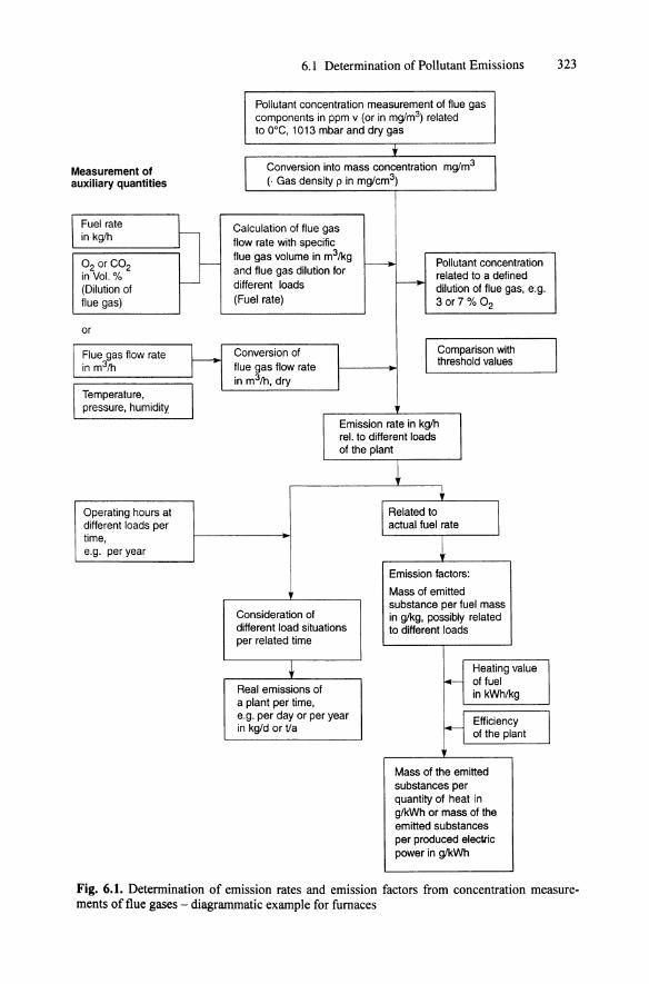
The means of determining emission flows and so-called emission factors from concentration measurements in exhaust gases is illustrated in Fig. 6.1 with the example of exhaust gases from furnaces. The determination of emission flows and emission factors in industrial production plants is, in principle, carried out in much the same

G. Baumbach, Air Quality Control© Springer-Verlag Berlin Heidelberg 1996

6.1 Determination of Pollutant Emissions 323

Pollutant concentration measurement of flue gas components in ppm v (or in mg/m3) related to O°C, 1013 mbar and dry gas ,

Measurement of Conversion into mass concentration mg/m3

auxiliary quantities (. Gas density p in mg/cm3)

Fuel rate ~ Calculation of flue gas in kg/h

flow rate with specific

02 or CO2 I--flue gas volume in m3/kg -- Pollutant concentration

in Vol. % and flue gas dilution for - related to a defined (Dilution of

f-- different loads dilution of flue gas, e.g. flue gas) (Fuel rate) 3 or7 % 02

or

Flue gas flow rate }- Conversion of Comparison with

in m3/h flue gas flow rate threshold values

in m3/h, dry Temperature, pressure, humidity

Emission rate in kg/h reI. to different loads of the plant

+ Operating hours at Related to different loads per actual fuel rate time, e.g. per year

Emission factors:

Mass of emitted substance per fuel mass

Consideration of in g/kg, possibly related different load situations to different loads per related time

~ Heating value

Real emissions of f- of fuel

a plant per time, in kWh/kg

e.g. per day or per year H Efficiency I in kg/d or tla of the plant

Mass of the emitted substances per quantity of heat in g/kWh or mass of the emitted substances per produced electric power in g/kWh

Fig. 6.1. Determination of emission rates and emission factors from concentration measurements of flue gases - diagrammatic example for furnaces

324 6 Evaluation of Air Pollution Measurements

way. Instead of dealing with fuel flows, production flows are to be dealt with. When trying to determine emissions in motor vehicles the matter is somewhat more complicated, as measurements are rarely carried out on vehicles in traffic and the different driving conditions must be simulated on roller dynamometers instead, s. [3-6].

The emission flows can be determined within the error limits described in sect. 5.6.5. Greater errors are to be expected when the emission factors are applied to other plants, as the emissions of different components, e.g., NO., depend heavily on individual combustion conditions.

When determining pollutant emissions (CO, CoRm' soot) stemming from instationary combustion conditions, which are formed, e.g., during incomplete combustion, the error is magnified. These substances develop, e.g., when starting or closing down furnaces and during break-downs. For these cases the individual determination of the flue gas volume flow is highly inaccurate - in the majority of cases even impossible. In domestic furnaces with solid fuels the individual degree of charging and burn out enter into the calculation. If even determining the emission flows of the components CO, CnRm and soot gives rise to problems, it is obvious that the determination of emission factors which are transferable to other plants can only represent a rough estimation.

Considering these points of view the emission factors mentioned in literature [7,8] should be assessed and used carefully.

6.1.2 Calculation of Pollutant Emissions from Fuel Properties

6.1.2.1 Sulfur Dioxide

As was shown in chap. 2 the sulfur bound in fuels burns almost completely to sulfur dioxide. The latter is emitted or, in some coal combustion processes, bound into the ashes (s. Table 2.4). It is advisable to calculate the S02 emission flows from fuel flows or fuel consumption. Precondition for this is, that the sulfur content of the fuels is known and does not change in the time relevant. When carrying out the calculation the following molecule balances must be considered:

S+02 = S02

1 Mol + 1 Mol = 1 Mol

32 g + 32 g = 64 g

1 g + 1 g = 2 g.

Thus, 2 g S02 are formed from 1 g bound sulfur.

(6.1)

(6.2)

(6.3)

(6.4)

Example: 1 kg of light fuel oil with a sulfur mass content of 0.2 % is burnt~ 4 g S02 are formed from 2 g of sulfur.

From the consumptions of individual fuels the S02 emissions of an entire area can be calculated relatively accurately for a defined period of time. The emission


values by the German Environmental Protection Agency are based on such calculations [9].

These calculations, however, become inaccurate if the sulfur content of the fuels are not known exactly. For light fuel oil, for instance, a maximum sulfur content of 0.2 mass proportion in % was prescribed [10], and calculations were usually carried out using this amount. The mineral oil industry, however, stated that the sulfur content of some light fuel oils was lower and that the average for the oil commercially available supposedly amounted to 0.24 % in 1984 [11].

The accuracy of the SOz emission calculations also decreases the more flue-gas desulfurization equipment is used. As these desulfurization units are at varying technological levels and have different removal efficiencies, measurements must be carried out directly in the flue gas when determining SOz emission flows. For this, the considerations on methods of determination and accuracy made in the previous chapter apply.

6.1.2.2 Nitrogen Oxides

As was shown in sect. 2.1.3 it is not possible to calculate nitrogen oxide emissions from the nitrogen content of the fuel. For one thing, not all of the fuel nitrogen is transformed into nitrogen oxide during combustion, for another, more or less atmospheric nitrogen is oxidized into nitrogen oxide depending on the combustion temperature.

When calculating flames and furnace dimensions it is advisable to calculate NO, emissions beforehand. However, this is only feasible for furnaces with defined dimensions and with known fuel properties [12, 13]. These models are at a stage where results calculated with them must be compared and verified with measured results. When applying the results of one furnace to another, furnace dimensions, fuel properties and load conditions would have to be included in the calculation process. The purpose of such computation models is not to collect emission data for NO, but rather to calculate in advance NO. emissions of furnaces at the planning stage so as to be able to design the construction of the burner and the furnace chamber such that NO. emissions are kept at a minimum.

When determining NO. emission flows from the many different plants one is therefore as dependant now as before on measurements in flue gases.

6.1.2.3 Products of Incomplete Combustion (PIC)

It is not possible to determine products of incomplete combustion (CO, CnHm and soot) from fuel properties as the emissions of these substances are influenced almost exclusively by the combustion process. Only a rough estimation of emission is possible by using emission factors determined at similar furnaces.

6.1.2.4 Heavy Metal Emissions in Oil Furnaces

While soot and total dust emissions in oil furnaces cannot be calculated from fuel properties, the metals contained in the oil can be determined in the flue gases as


oxides. It has, however, not yet been checked whether this determination is quantitatively possible [14]. Particularly when burning heavy fuel oils metal emissions have a special significance. Nickel and vanadium oxides, for instance, are emitted in the process. When tracing atmospheric pollutants these metals can serve as indicators of flue gas components from heavy oil furnaces [15].

In light fuel oils metals occur only in the slightest of concentrations so that the emissions of the relevant oxides have as yet had no significance. Up until now lead was added to gasoline in the form of lead tetraethyl as an antiknock agent. The lead emissions of the motor vehicles correspond to the lead content of the gasoline used and can be extrapolated from them. However, that does not tell us in which form the lead is emitted. E.g., halogenous compounds are added so that lead compounds volatilize easier.

When burning coal there is a high degree of ash components in the flue dust. However, the fact that part of the ash is already retained in the furnace chamber and the largest part of the flue ash is kept back in the flue gas particle precipitators makes calculating particle emissions from fuel composition impossible. For coal furnaces particle emissions can only be determined by flue gas measurements.

6.1.3 Registering Pollutant Emissions of an Area in Emission Inventories

6.1.3.1 Spatial Pollutant Distribution

To be able to recognize relationships between emissions and pollutants in a certain area it is important to begin by compiling an overview of the dispersion of pollutant emissions of the area concerned. In these emission inventories the extent of the emissions from the different main source groups is listed: - motor vehicle traffic, - domestic furnaces and those of small-scale industries, - industry: furnaces including power plant furnaces and industrial processes.

For these inventories the area to be assessed is usually divided into subsections of 1 x 1 km and pollutant emissions released in these areas are calculated per annum. Emission conditions are depicted graphically by coloring these subsections in topographical maps. Owing to this type of presentation one can, e.g., infer from these maps in which sections of a town high amounts of pollutants are released and where emissions are low. In combination with air quality inventories areas can be identified where air pollution control measures should be preferably taken. Therefore emission and air quality inventories are vital components of air quality control concepts.

The temporal dispersion of the pollutant emissions cannot immediately be inferred from the inventories. It must be calculated separately and according to [8] it is to be shown also for the period of one calendar year with the proportions of the individual emittents visibly marked.


Pollutants

According to [8] the following atmospheric pollutants, in particular, are to be included in the emission inventories: - particulate, - fine particles <0.01 mm (aerodynamic diameter up to 85 % <0.01 mm), - lead and lead compounds - listed as Pb, - sulfur dioxide (S02)' - nitrogen dioxide - listed as N02, - carbon monoxide (CO), - gaseous and vaporous organic compounds, - chlorine and gaseous anorganic chlorine compounds - listed as Ct, - fluorine and gaseous anorganic fluorine compounds - listed as F-.

Frequently, there are no measuring data available on the individual pollutants emitted, particularly for the not so common pollutants (e.g., fine particles, organic compounds, Cl- and F-). Therefore, the values used are usually based on estimates or emission factors based on them. Thus, great accuracy may not be expected here.

6.1.3.2 Determination of Pollutant Emissions of Motor Vehicle Traffic

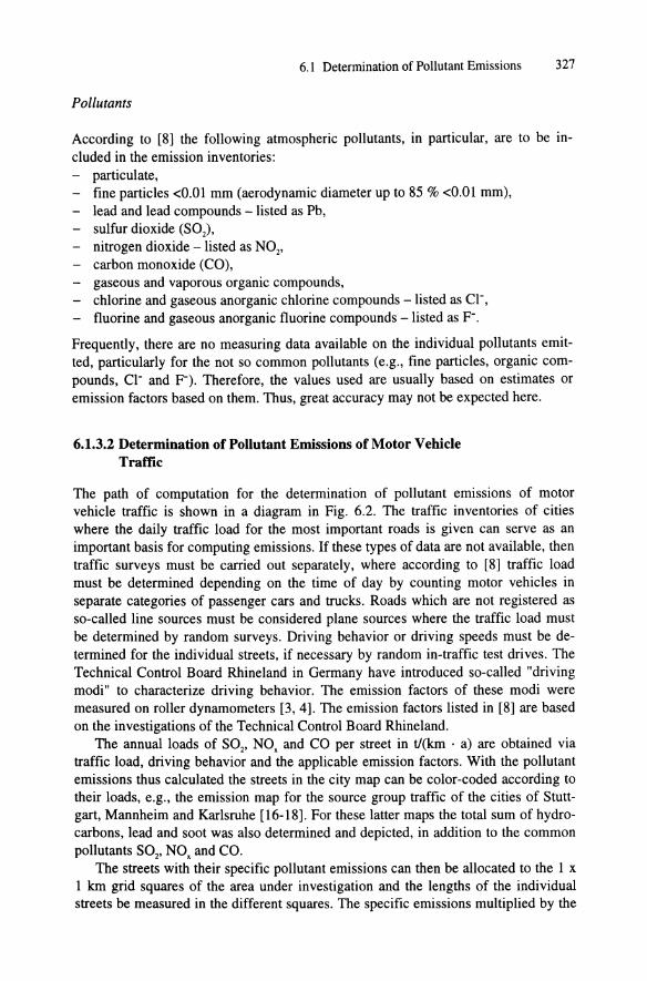
The path of computation for the determination of pollutant emissions of motor vehicle traffic is shown in a diagram in Fig. 6.2. The traffic inventories of cities where the daily traffic load for the most important roads is given can serve as an important basis for computing emissions. If these types of data are not available, then traffic surveys must be carried out separately, where according to [8] traffic load must be determined depending on the time of day by counting motor vehicles in separate categories of passenger cars and trucks. Roads which are not registered as so-called line sources must be considered plane sources where the traffic load must be determined by random surveys. Driving behavior or driving speeds must be determined for the individual streets, if necessary by random in-traffic test drives. The Technical Control Board Rhineland in Germany have introduced so-called "driving modi" to characterize driving behavior. The emission factors of these modi were measured on roller dynamometers [3, 4]. The emission factors listed in [8] are based on the investigations of the Technical Control Board Rhineland.

The annual loads of S02' NO, and CO per street in t/(km . a) are obtained via traffic load, driving behavior and the applicable emission factors. With the pollutant emissions thus calculated the streets in the city map can be color-coded according to their loads, e.g., the emission map for the source group traffic of the cities of Stuttgart, Mannheim and Karlsruhe [16-18]. For these latter maps the total sum of hydrocarbons, lead and soot was also determined and depicted, in addition to the common pollutants S02' NO, and CO.

The streets with their specific pollutant emissions can then be allocated to the 1 x 1 km grid squares of the area under investigation and the lengths of the individual streets be measured in the different squares. The specific emissions multiplied by the

I

I

l

I

I

I


Traffic load inventory ~ Registration and

Non-registered roads of ~ numbering of the roads

city map

Traffic load/day; I proportion of trucks I

Annual traffic load per road for passenger cars and lorries

Assessment of driving I modes I Emission factors accor- I ding to the driving modes I

Annual 802 and NOx Color-coded representation - of high-emission roads

emission per road t/(km . a) in city map

Division of city area into I grid squares of 1 x 1 km I

Allocation of individual street sections to the grid squares

Annual 802 and NOx emission of traffic per grid square in tI(km2 . a)

Fig. 6.2. Calculation mode for determining the S02 and NO, emissions from traffic per road and per square kilometer in a city (also valid for other compounds)

relevant street length give the annual emissions of each street per determined square kilometer. The sums of all streets of a grid square then represent the pollutant emissions in tJ(km2.a) caused by motor vehicle traffic [16-18].

6.1.3.3 Pollutant Emissions of Domestic Furnaces and SmallScale Industries

The 5th Administrative Regulation for the Implementation of the Federal Air Pollution Control Act [8] stipulates that the number and type of furnaces, the fuels used, the nominal capacities of the furnaces, the source heights and the geographic position are to be determined. For this, the data secured by the chimneys weeps on their an-


nual check of domestic furnaces is to be used as far as possible. Determining the number of furnaces, however, is relatively complex. The accuracy thus achieved is partially undone by the fact that there are no data available on the fuel consumptions of the furnaces and that estimates must be made for this as the furnace capacity does not necessarily say anything about its degree of utilization.

Occasionally, studies on district heating also include data on heat requirement densities of individual town sections. If the annual heat supplies of gas and piped heat are known (these can be obtained relatively easily), then the consumption of light fuel oil can be estimated by calculation. Pollutant emissions can thus be determined for the inventories via the individual heat consumptions and with the help of emission factors. E.g., an air quality control concept for the city of Heilbronn, Germany, was carried out in this way [19].

Fig. 6.3 shows the computational method applied for this. When drawing up the official administrative emission inventories in Germany surveys were not carried out with the utmost consistency, the final energy consumptions being determined via computational methods similar to the one shown in Fig. 6.3 instead [20, 21].

In his "Manual on the Setting up of Clean Air Plans" [22] Dreyhaupt gives directions on how to carry out statistical surveys in large urban areas without interviewing all households (a so-called microcensus).

As an example an emission inventory was drawn up for a small town for which approximately 70 % of all households were individually interviewed to collect data on type of fuel and annual fuel consumption [23]. An emission inventory compiled in this manner naturally surpasses all other survey methods in accuracy. However, it cannot be implemented in larger towns as it is very work-intensive.

Pollutant emissions from small-scale industries depend on the materials used, on the type of construction and the mode of operation of the furnaces. The following businesses shall be listed as examples: gasoline stations, printing shops, dry cleaners, paint shops, woodworking, smokehouses, light fuel oil depots and plants for the treatment of parts with chlorinated hydrocarbons. Dreyhaupt [22] gives detailed instructions on how to collect data for this purpose, too. To do this, questionnaires must cover all types of plants. The calculation of the emissions is carried out, e.g., with the help of specific emission factors and the amount of produced or consumed materials.

6.1.3.4 Pollutant Emissions from Industries

When compiling an emission inventory for Industry one cannot avoid individually interviewing all plant operators. In the "polluted areas" for which the authorities must set up an air quality control concept the operators of "plants requiring official approval" [24] must make so-called emission statements [25]. The emission statements are requested by the approving authorities, e.g., the industrial inspection boards. Apart from the information covering the plants operating hours, the types and amounts of materials used (e.g., fuel consumptions), direct statements pertaining to the emission flows must be made. The emission statement is to be up-dated every two years.


Marking of the areas supplied with heat and listing of the heat supply densities and supplying values

Heat utilization in h/a

Heat consumption per year in the single districts

District heat supply I per year I

Gas supply per year in the single districts

~ ~ District heat Gas portion Heat consumption

portion - District heat portion - gas portion

Light oil portion

1 r Gas consumptions/year I Oil consumption/year

Division of city area I into grid squares (1 x 1 km)

Allocation of the areas supplied to the grid squares

Calculation of gas and oil consumption in the single grid squares

Emission factors of gas and oil combustion in kg/MWh

Annual S02 and NOx emissions of domestic heating and small consumers per grid square in t/(km2 . a)

Fig. 6.3. Calculation mode for determining S02 and NOx emissions from domestic heating systems per square kilometer [19]


The annual emissions of the plants are either determined from the individual emission flows by mUltiplying them with the operating hours, or they are calculated, e.g., in industrial furnaces, from the fuel consumption with the help of specific emission factors. Depending on the location of the individual plants the pollutant emissions thus determined are allocated to the grid squares of the survey area and are color-coded in the emission inventory maps [26, 27].

6.1.3.5 Summary of Annual Emissions

To determine their spatial dispersion the pollutant emissions of the individual source groups are combined for each square kilometer of the surveyed area (based on the 1 x 1 kIn Gauss-Krueger grid l ) and color-coded according to their concentrations. In this way the emission inventory maps were set up for the polluted areas as being essential to the air quality control concepts [28-30]. As an example the emission dispersion of the pollutant NO. (NO+N02) determined and depicted in the manner described is shown for the town of Heilbronn, Germany, s. Fig. 6.4 [19].

As can be seen, the highest NO. emissions come from a power plant, even if emitted via high stacks. Besides these power plant emissions the highest emissions occur in the inner city area on the one hand and in the northern part of the town near a highway on the other. This NO. emission dispersion which is mainly caused by motor vehicle traffic is typical of urban areas. In areas with high traffic densities which unfortunately occur frequently in the city centers along with high residential density traffic-related pollutant emissions (NO., CO, hydrocarbons) are also at their highest level. Apart from these, highways with heavy traffic represent large nitrogen oxide sources.

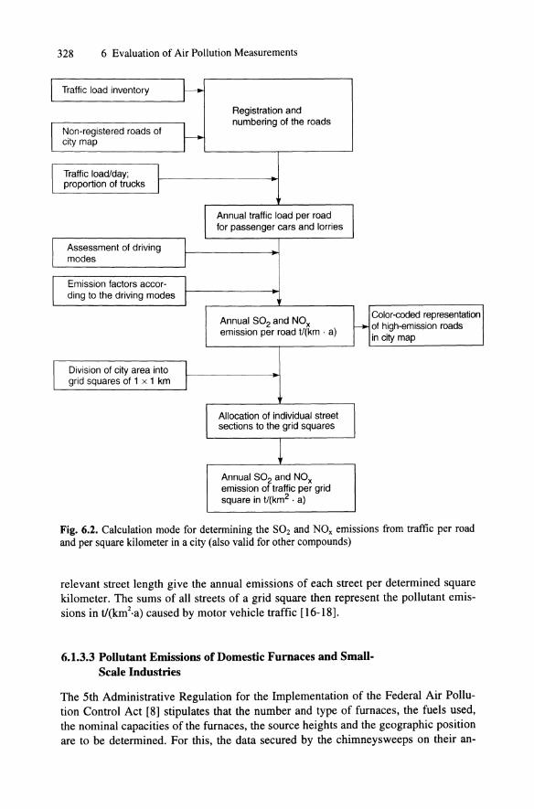
The emissions of the different source groups do not become effective as pollutants to the same extent due to their varying source heights (motor vehicle exhausts directly in the respiratorial space, industrial stacks up to a height of 250 m). It is therefore attempted to weight the emissions according to their individual contribution of pollution to the ambient air. For this, apart from the source heights, the different weather conditions which influence the dispersion of the pollutants are included. After comparing dispersion calculations and pollution measurements Kutzner [31] has defined so-called pollution assessment factors for the different emission sources for the example of Berlin. Assessments of this type [19, 29] can occasionally be found in air quality control concepts. Such an assessment for the pollution component NO. is shown graphically in Fig. 6.5. It must however be admitted, that the values indicated for the polluted areas are rough estimates and rough mean values for an entire urban area (there are definite local differences). Such considerations, however, can be of help in deciding on pollution control measures.

1 In topographic maps the 1 x 1 Ion Gauss-Krueger grid is plotted with the coordinates of the x- and y-axis.


I:S:3 No emissions W1l1l:B 91 ... 120 Va

l2Zl 0 ... 30Va [;kdM > 120 Va

fQS2SI 31 ... 60 Va liD] > 1000 Va

c::J 61 ... 90 Va c::J Outside of examined area

Fig. 6.4. Distribution of NO. emissions in the city ofHeilbronn, FRG [19]

6.1.3.6 Temporal Pollutant Distribution

To determine relationships between emissions and pollution a fine temporal resolution is often useful. For pollution in urban areas, e.g., characteristic diurnal courses can be determined which are on the one hand created by meteorological dispersion conditions such as height of mixed layer, but on the other hand the emission diurnal course has a considerable influence on the pollution profile. Thus, at least for research which aims at tracing atmospheric pollution from emission to deposition it is important that diurnal courses of emissions are known with an hourly or half-hourly resolution.

~ 0

,S (JJ c 0

'';::;

0 0-(JJ C 0 'Vi (JJ

'E ill

80

60

40

20

Emissions portions

c:::::::J Remaining

EZ2Z3 Power stations

cs::::J Traffic

Average of all weather conditions


- Load portions in city-

Weather conditions with low exchange and low inversion height

II!!II1B Industry

Weather conditions with low exchange and medium height of inversion

I i i Domestic heating

Fig. 6.5. Emissions of source groups traffic, domestic heating, industrial furnaces and power plants with their contribution to air pollution in an urban area (example for the component NOx)[19,32]

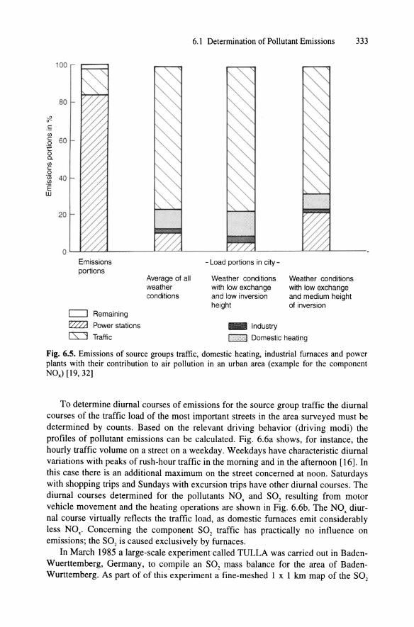
To determine diurnal courses of emissions for the source group traffic the diurnal courses of the traffic load of the most important streets in the area surveyed must be determined by counts. Based on the relevant driving behavior (driving modi) the profiles of pollutant emissions can be calculated. Fig. 6.6a shows, for instance, the hourly traffic volume on a street on a weekday. Weekdays have characteristic diurnal variations with peaks of rush-hour traffic in the morning and in the afternoon [16]. In this case there is an additional maximum on the street concerned at noon. Saturdays with shopping trips and Sundays with excursion trips have other diurnal courses. The diurnal courses determined for the pollutants NO. and S02 resulting from motor vehicle movement and the heating operations are shown in Fig. 6.6b. The NO. diurnal course virtually reflects the traffic load, as domestic furnaces emit considerably less NO •. Concerning the component S02 traffic has practically no influence on emissions; the S02 is caused exclusively by furnaces.

In March 1985 a large-scale experiment called TULLA was carried out in BadenWuerttemberg, Germany, to compile an S02 mass balance for the area of BadenWurttemberg. As part of of this experiment a fine-meshed 1 x 1 km map of the S02


IJ)

-'" ()

S "0 c

'" ~ '" ()

Oi OJ c Q) IJ) IJ)

'" a. '0 Oi .c E ::J Z

a

.~ IJ) c o 'w IJ)

'E UJ

N o (j)

"0 C

'" OX z

b

600.---------------------------------------------------~

500

400

300

200

100

0

12

10

8

6

4

2

Trucks ............ ; .............. / ......... ..

Passenger cars

....... . ........... : : ..... : ... , .. .

000

._._.J'

NOx Motor vehicles

802 Furnaces

NOx Furnaces

802 Motor vehicles

r'

S·J

-~ ..... S

000 600

1200

Time of day

1200

Time of day

1800

'::;L . .., 1....,

L.""L.

Fig. 6.6. Diurnal variation of vehicle number (a) NOx and S02 emissions (b) during a working day in a small town [23]

6.2 Evaluation and Graphic Representation of Air Quality Measurements 335

and NO. emissions with an hourly resolution was drawn up [33, 34]. The emissions of small furnaces were computed with models based on the evaluation of data of the ambient conditions. For the larger industrial plants emission rates were determined by interviews.

The profiles of the NO. emissions in Baden-Wuerttemberg during the two weeks of this field experiment are shown in Fig. 2.18 as an example of this evaluation. The large share of motor vehicle emissions with completely specific diurnal courses are to be seen: peaks in the mornings and in the afternoons, at night always a drop to lowest values. The two lower peaks in the middle of the diagram indicate the lower week-end traffic. The biggest part of these motor vehicle-related NO. emissions comes from the urban areas and from the country's highly frequented highways.

Knowing the spatial and temporal structure of the pollutant emissions can in many cases explain why ambient air pollution occurs.

6.2 Evaluation and Graphic Representation of Air Quality Measurements (with K. Baumann)

Concentrations of the different air pollutants can be subject to marked fluctuations as far as time and space are concerned. It is the task of measuring technology to obtain as much information as possible on this.

Depending On the problem at hand different measuring plans can be set up and differentiated evaluations and graphic representations of the pollution measurements can be carried out. Instructions on setting up measuring plans can, e.g., be found in the 4th General Administrative Regulation for the Implementation of the Federal Air Pollution Control Act "Determination of Air Quality in Polluted Areas" [35]. It should be noted that the layout of the measuring plan and the representation of the results can even imply an evaluation of the results. The following sections will provide possibilities of evaluating and graphically representing measured data.

6.2.1 Temporal Resolution and Mean Value Formation

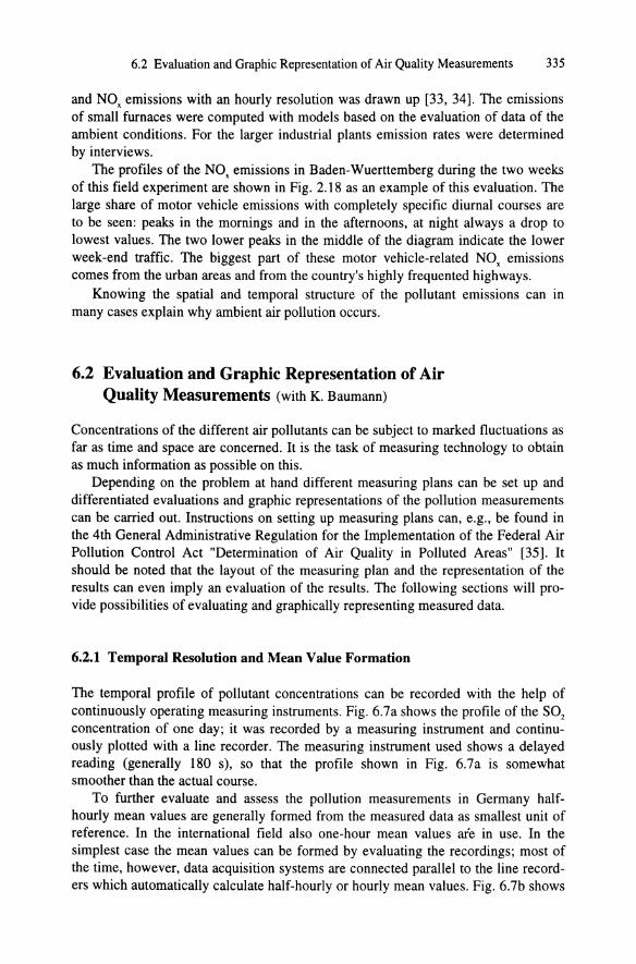
The temporal profile of pollutant concentrations can be recorded with the help of continuously operating measuring instruments. Fig. 6.7a shows the profile of the S02 concentration of one day; it was recorded by a measuring instrument and continuously plotted with a line recorder. The measuring instrument used shows a delayed reading (generally 180 s), so that the profile shown in Fig. 6.7a is somewhat smoother than the actual course.

To further evaluate and assess the pollution measurements in Germany halfhourly mean values are generally formed from the measured data as smallest unit of reference. In the international field also one-hour mean values ate in use. In the simplest case the mean values can be formed by evaluating the recordings; most of the time, however, data acquisition systems are connected parallel to the line recorders which automatically calculate half-hourly or hourly mean values. Fig. 6.7h shows


1000~--------------------------------------------------.

E 800

~ 600 c '" 400

55 200

1000 '" E 800 e,

600 :::l. .!: 400 '" 0

200 en

1000 '" E 800 l-e, :::l. 600 l-.!:

'" 400 I-0 en 200 l-e 0

1000 '" .§ 800 I-Ol :::l. 600 I-

.!:

'" 400 I-0 en 200 I-

0 d 000

,I .I

Time of day

Fig. 6.7. Example of S02 measurement over 24 hours with different averaging times [36]. a. continuous measurement, b. half-hour, c. 3-hour, d. 24-hour averaging

the concentration profile of Fig. 6.7a, averaged with half-hourly values. If three hourly mean values are formed from the profile which, e.g., are the time basis in smog alarm plans, then there is a concentration profile as shown in Fig. 6.7c. The daily mean value (24 hour mean value) is shown in Fig. 6.7d. As can be seen, averaging the values causes a loss of information on the structure of the temporal profile.

The temporal averagings can also be the result of the measuring technique used. Very low concentrations in outside air, for instance, can sometimes only be measured by enriching them through longer sampling times. In this way particle concentrations, e.g., are sometimes recorded as daily mean values [37].

The extent of the temporal resolution of air quality measurements depends on their biological effect, or on any other effect which is to be investigated or which is to be cautioned against via this measurement.

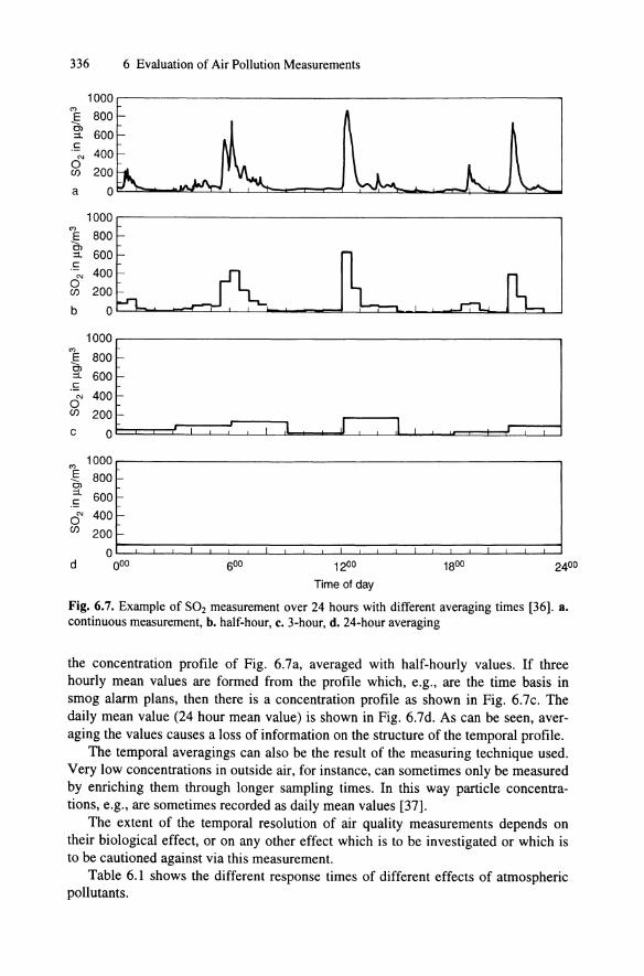
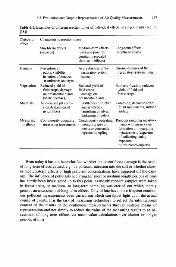
Table 6.1 shows the different response times of different effects of atmospheric pollutants.


Table 6.1. Examples of different reaction times of individual effects of air pollutants (acc. to [38])

Objects of Characteristic reaction times effect

Short-term effects Medium-term effects Long-term effects (seconds) (days and possibly (months to years)

constantly repeated short-term effects)

Humans Perception of Acute diseases of the chronic diseases of the odors, visibility, respiratory system respiratory system, lung irritation of mucous cancer membranes and eyes

Vegetation Reduced yield of Reduced yield of Soil acidification, reduced field crops, damage field crops, yield of field and on ornamental plants damage on forest crops (acute necroses) ornamental plants

Materials Acid-caused pit corro- Brittleness of rubber Corrosion, decomposition sian destruction of and synthetics, of art monuments, surface nylon fibers tarnishing of silver, soiling

darkening of colors Measuring Continuously operating Continuously operating Random sampling measure-

methods measuring instruments measuring instruments with mean value ments or constantly formation or integrating repeated sampling measurement (exposure

of collecting tanks, exposure oftest pieces/objects)

Even today it has not been clarified whether the recent forest damage is the result of long-term effects caused, e.g., by pollutant intrusion into the soil or whether shortor medium-term effects of high pollutant concentrations have triggered off the damage. The influence of pollutants occurring for short or medium length periods of time has hardly been investigated up to this point, as mostly random samples were taken in forest areas, or medium- to long-term sampling was carried out which merely permits an assessment of long-term effects. Only of late have more frequent continuous pollutant measurements been carried out which can throw light upon the actual course of events. It is the task of measuring technology to reflect the informational content of the results of the continuous measurements through suitable means of representation and not simply to reduce the value of the measuring results to an assessment of long-term effects via mean value calculations over shorter or longer periods of time.


6.2.2 Summary and Graphic Representation of Measuring Data from Continuous Measurements

6.2.2.1 Unsmoothed Monthly Profiles

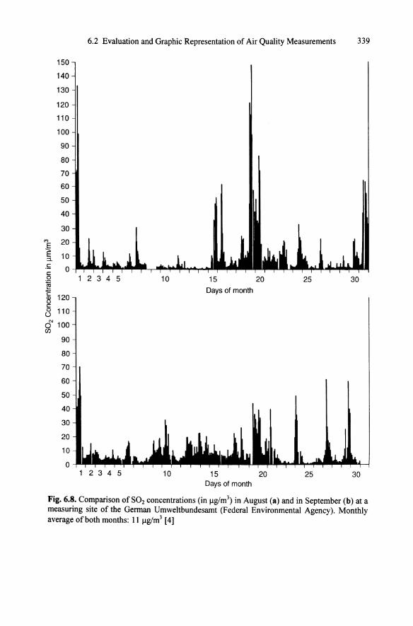
For the representation of its measuring results the Environmental Protection Agency of Germany has chosen as smallest unit of reference mean values of 1 hour [37]. A complete graphic representation of all I-hour mean values for one month is shown in Fig. 6.8. Every I-hour mean value is plotted as a vertical line, so that all peaks, all low values and all failures of measurement are recognizable. Such a compact representation saves considerably more space than the plottings of a continuous-line recorder and can be grasped at a glance, which is not the case with tables. Fig. 6.8 compares the S02 concentration recordings for two months of the German measuring site Waldhof. In both months a monthly mean value of 11 ~g/m3 was calculated from the individual values. These graphic representations show how by solely indicating mean values actual events can become blurred: in August 1983 there were two peak concentrations of 130-150 ~g/ml, whereas in September very brief peaks amounted to only 70 ~g/m3. The different monthly profiles are with certainty different in their relevance of effects.

6.2.2.2 Mean Value Calculation for Smog Warnings

To assess smog hazards sliding 3-hourly mean values are formed from the halfhourly values measured as usual. In this case sliding means, that after every newly measured half-hourly value the previously calculated 3-hour mean value is updated. In the smog regulations of Germany [39] 3-hour threshhold values are fixed for different alarm phases; when these are exceeded the appropriate smog warning is to be issued. E.g., a smog warning must be given when two measuring stations in a town record values exceeding 0.6 mg/mJ of S02 or 0.6 mg/ml of N02.

Moreover, the smog regulations also provide threshold values for a 24-hour averaging time. In this, the measured air-borne particulate concentration is included in the assessment.

6.2.2.3 Diurnal Courses

If specific situations are to be investigated in greater detail, then pollutant profiles are usually shown as diurnal courses based on half-hourly values (s. Fig. 6.7b). As an example of special situations Fig. 6.9 compares the concentration profiles of a day with an inversion and a rainy day. The diurnal courses of wind speed are also included. As can be seen, there are only low wind speeds on the inversion day. When the wind speed picks up some in the early afternoon pollutant concentrations immediately decrease. On the rainy day there is a strong wind throughout the whole day and the pollutants provide only low values. The concentration increase in the morning hours is not a result of unfavorable exchange conditions but of the rush-hour


150

140

130

120

110

100

90

80

70

60

50

40

30

'" 20 E E 10 :::1. .£; 0 c: 0 1 2 3 4 5 10 15 20 25 30 ~

Days of month C Q) 120 u c: 0 110 0

0'" 100 (j)

90

80

70

60

50

40

30

20

10

0 1 2 3 4 5 10 15 20 25 30

Days of month

Fig. 6.S. Comparison of S02 concentrations (in llg/m3) in August (a) and in September (b) at a measuring site of the German Umweltbundesamt (Federal Environmental Agency). Monthly average of both months: II llg/m3 [4]


7

---- NO q '" nil 0 CO II I L, z

6 0 6 ............. N02 III I () z ~II I q Wind

II I 15 0.5 II rJ I I I 5 II

p II I I I I I L...J I fl I I I I I

12 0.4 I L, II I I I L, 4 .!!?

III II d E > r..l L .£ E ;;I "l., II I LJ "0 C. ILJ Q) c. I Q)

.£ 9 0.3 l I I 3 c. <Jl

I:: "l., n"l..J I "0 0 L_J I I:: ~ ~ l:; I I:: Q)

6 0.2 2 0 I:: 0 ()

3

0

a

0 ()

12

> E 8:9 .£ I:: .Q '§ "E 6 ~ I:: 0 ()

3

o

b

0.1

L-~~~ __ ~ ________ ~ __________ ~~L-______ ~O

1200

Time of day 2400

'" 'r---------------------------------------------,5 0 z ---- NO 6 z ---CO

0.4 ............. N02

0.3

0.2

0.1

r-' '--.'-"""L ", ... .r"\. '''',,-_

o ::: _____ -:.~-::.~.:.-=.-............... -.......... -: .. -.'k ...................... .,........ ·"'-... ---.. ..... _ .. ··, ........ u __

000 600 1200 1800

Time of day

4

~ 3 .£

1 2 "0

I::

o 2400

~

Fig. 6.9. Comparison of diurnal courses of the pollutants NO, N02, CO and wind speed on a day with inversion (a) and on a rainy day (b) - measurements were taken at a high traffic road [40]


traffic peak during this time of day. This fact can be confirmed by a comparison with the diurnal course of the traffic load [40].

6.2.2.4 Long-Term Annual Profiles

In the simplest method of representing the pollutant profiles of several years the annual mean values are included graphically, s. [41]. However, one does not obtain a lot information from this as concentrations can fluctuate considerably within one year.

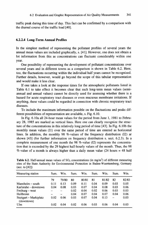
One possibility of representing the development of pollutant concentrations over several years and in different towns as a comparison is shown in Table 6.2. Here, too, the fluctuations occurring within the individual half years cannot be recognized. Further details, however, would go beyond the scope of this tabular representation and would make it less clear.

If one takes a look at the response times for the atmospheric pollutants listed in Table 6.1 to take effect it becomes clear that such long-term mean values (semiannual and annual values) cannot be directly used for assessing whether there is a hazard for acute respiratory tract diseases or even mucuous membrane irritations. If anything, these values could be regarded in connection with chronic respiratory tract diseases.

To include the maximum information possible on the fluctuations and peaks different possibilities of representation are available, s. Fig. 6.10.

In Fig. 6. lOa all 24-hour mean values for the period from June 1, 1981 to February 28, 1985 are marked as vertical lines. Here one can clearly recognize the structure of the concentrations in this relatively long period of time [43]. In Fig. 6. lOb the monthly mean values (11) over the same period of time are entered as horizontal lines. In addition, the monthly 98 %-values of the frequency distribution (12) ar shown [43] (for further information on frequency distribution s. sect. 6.2.3). In a complete measurement of one month the 98 %-value (12) represents the concentration that is exceeded by the 29 highest half-hourly values of the month. Thus, the 98 %-value of a month is always higher than a daily mean value (24 hours = 48 half

Table 6.2. Half-annual mean values of S02 concentrations (in mg/m3) of different measuring sites of the State Authority for Environmental Protection in Baden-Wuerttemberg; Germany (acc. to [42])

Measuring station Sum. Win. Sum. Win. Sum. Win. Sum. Win.

79 79/80 80 80/81 81 81182 82 82/83 Mannheim - south 0.11 0.13 0.09 0.11 0.04 0.09 0.03 0.05 Karlsruhe - downtown 0.04 0.08 0.03 0.07 0.04 0.08 0.03 0.06 Freiburg - west 0.02 0.04 0.02 0.06 0.03 0.03 Heilbronn 0.04 0.07 0.04 0.07 0.04 0.06 Stuttgart - Marktplatz 0.02 0.06 0.03 0.07 0.04 0.13 0.03

(downtown) Vim 0.02 0.04 0.02 0.06 0.03 0.06 0.04 0.03

342

'" E 0, E 8 .£ c: 0

4 ~ "E (]) t.>

0 c: 0 ()

'" 12 E 0, E .£ 8 c: 0

~ "E 4 Q) t.> c: 0 ()

0

150

'" -§, 120 :::t

.£ c: 0

~ "E Q) t.> c: 0 U

~ :::t

.£ c: o ~ E

90

60

30

0

200

~ 100 c: o U

0'"

o

6 Evaluation of Air Pollution Measurements

CO 24-hour averages

1981 1982 1983 1984 1985

CO Month averages q I I I I I I fl r1 I I r-J LI2 I I r-' I

rJ L, I I I r--J LJ L_, r1 r--' L ___ ,

,r ... .r .... .r-' L_J U L __ J 11

o J o J o J o J 1981 1982 1983 1984 1985

S02 157

Highlands in Southern Germany

-~ Jan. Jan. Jan. 10 20 30

1985 1986 1987 January 1987

0 3

l-

I

r~ 1 1 1 ~ 1 I

J OJ OJ OJ OJ o 1984 1985 1986 1987 1988


hours). The representation in Fig. 6.lOc is similar to the one in Fig. 6. lOb, except that instead of the 98 %-values (12) the highest daily mean values (vertical lines on the left, polygonal course on the right) are plotted together with the monthly mean values (bars). In addition to the monthly mean values (bars) the highest half hourly values (vertical lines) are included with every month in Fig. 6.lOd [45].

6.2.3 Frequency Distribution

Graphic representation of frequency distribution serves to investigate how frequently certain pollutant concentrations occurred in a measuring period or measuring series. For this, the pollutant concentration is divided into the required number of classes on the abscissa, and the frequency of the measured values in the individual classes, either in their absolute number or in percent in reference to all measuring values is shown on the ordinate. Fig. 6.11 shows a frequency distribution of this type.

20~--------------------------------------------------~

15

5

o

Fl I

I I .... : : .... L:: :J r "'1 .J I c .. :

1

l-,

50

Near road 30 m distance 60 m distance

100 150

100 % = 6339 values 100 % = 6331 values 100 % = 6696 values

200

Concentration classes in l1g/m3

250 300

Fig. 6.11. Frequency distribution of an N02 measuring series near a highway, measuring cycle from April to November 1985

Fig. 6.10. Different possibilities of representing annual courses including information on maximum values; B. 24-hour mean values; b. monthly mean values (11) and monthly 98 % values (12); c. monthly mean values and highest daily mean value as well as polygonal curve of the daily mean values of a month; d. monthly mean values and highest half-hourly values [43-45]


Atmospheric pollutants generally have an asymmetrical distribution, i.e., there are many low measuring values and only a few high ones. The latter are, e.g., caused by low exchange weather conditions which are not very persistent in typical Central European weather conditions and do not occur very frequently. In this asymmetrical distribution the mean value of the measurement is generally not identical with the most frequent value (highest point of the envelope curve).

The frequency distribution is different for every measuring site; in sites close to a source it will be shifted to the right to higher concentrations as compared to sites far from sources. One can also see from the diagram how much the measuring values fluctuate. A slender envelope curve signifies slight, a wide envelope curve considerable fluctuations.

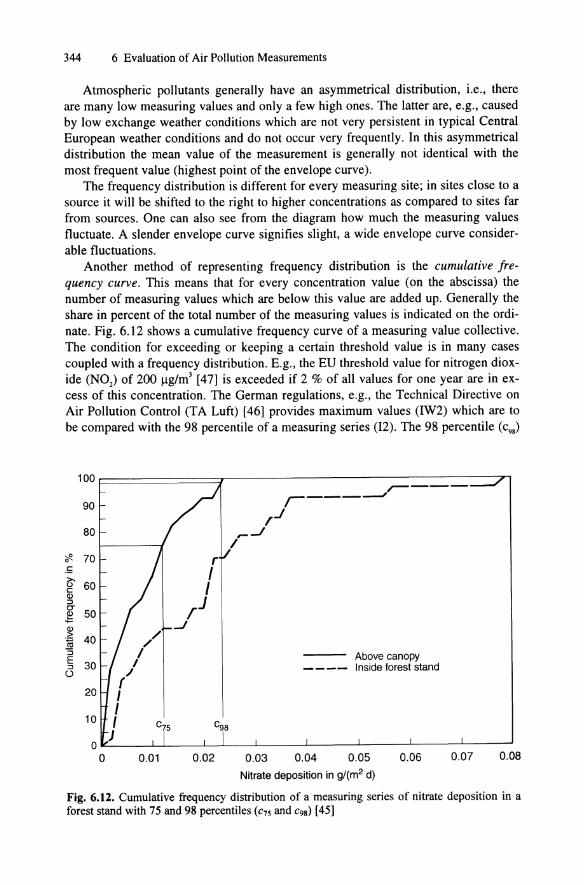
Another method of representing frequency distribution is the cumulative frequency curve. This means that for every concentration value (on the abscissa) the number of measuring values which are below this value are added up. Generally the share in percent of the total number of the measuring values is indicated on the ordinate. Fig. 6.12 shows a cumulative frequency curve of a measuring value collective. The condition for exceeding or keeping a certain threshold value is in many cases coupled with a frequency distribution. E.g., the EU threshold value for nitrogen dioxide (NOz) of 200 f.!g/mJ [47] is exceeded if 2 % of all values for one year are in excess of this concentration. The German regulations, e.g., the Technical Directive on Air Pollution Control (TA Luft) [46] provides maximum values (IW2) which are to be compared with the 98 percentile of a measuring series (12). The 98 percentile (c9S)

100

90

80

~ 0 70 .5 ()' 60 c Q) ::J 0-

50 ~ Q) > 40 .~

::; E 30 ::J 0

20 ( , I

10 I J

0 0

/ /

/ I

/

C75 cg8

0.01 0.02

,----, ___ --J

/J ,....J

I

0.03 0.04

Above canopy Inside forest stand

0.05 0.06

Nitrate deposition in g/(m2 d)

0.07 0.08

Fig. 6.12. Cumulative frequency distribution of a measuring series of nitrate deposition in a forest stand with 75 and 98 percentiles (C75 and C9S) [45]


is the concentration below which 98 % of all measuring values ar to be found, s. also Fig. 6.12. Thus, 2 % of all values are in excess of this concentration. Accordingly, the 98 percentile is, e.g., identical with the above-mentioned EU maximum concentration which is exceeded when 2 % of all values are in excess of it. Apart from the C98 value the C75 value has been marked in Fig. 6.12 which is the concentration which is not reached by 75 % of the measuring values or exceeded by 25 % of all values.

If the total number of the measuring values is known, it is possible to calculate how many measuring values exceed the threshhold concentrations (e.g., in excess of C75 or cg8). Percentile methods have become established in many institutions so that most of the time C98 values are shown in evaluations.

If the frequency distribution curve is known one use the threshold concentration on the abscissa as a basis; where the curve intersects with the ordinate one can see how many percent of the values are below this concentration. The percentage multiplied by the total number gives the number of the values which fall below the threshold concentration.

If one wants to determine excess frequencies then simply those values which lie above the desired concentrations must be counted in the evaluation. Table 6.3 gives an example of such an evaluation of S02 measurements in several measuring stations in a narrow valley where a factory is located [36]. The concentrations limits shown here are the threshold values of different organisations.

Other institutions, too, indicate excess frequencies in this tabular form, compare [48,49].

If excess frequencies are to be represented graphically, then the sum frequency curve is not so clear. This latter shows how many values are below a certain concentration - thus, this curve primarily shows frequencies remaining below these concentrationsd. Of course, excess frequencies can be calculated upto 100 % by determining the difference. But it is also possible to enter the percentage excess over the concentration directly. Fig. 6.13 shows an example of excess frequencies of different pollut-

Table 6.3. Number of S02 half-hour values exceeding the listed maximum values in the measuring period from October 1985 to March 1986; 4 S02 monitoring stations in a Black Forest valley [36]

Measuring Site Total number of Threshold Concentrations measured values

0.075" 0.15b

1 St6ckerkopftop 7327 349 162 2 St6ckerkopf middle 6142 462 206 3 SWckerkopf bottom 4629 27 12 4 Surrbachkopf 6541 440 87

" Threshold value of IUFRO for fir. b Threshold value ofIUFRO for spruce. c Threshold value acc. to VDI for highly sensitive plants. d Threshold value acc. to VDI for sensitive plants. • MIK value for the protection of human health.

0.25c

50 89

8 5

OAOd 1.0·

16 3 44 8

6 1 0 0


100 ----90 " NO 1 00 % = 9000 Values \ " -- N02 100 % = 8999 Values

80 . \ " _.- 8°2 1 00 % = 1 0548 Values , \ ---- 0 3 100 % = 10007 Values

~ 70 0 \ \ .5 ~ 60 \ c: . \ \ (]) \ :::I

\\ 0" 50 \ ~ \ Cl \ c: 40 ., 'C \ (]) (])

~\ " ~ 30

" w

" 20 "-10

0 0 50 150 200

Concentration in llg/m3

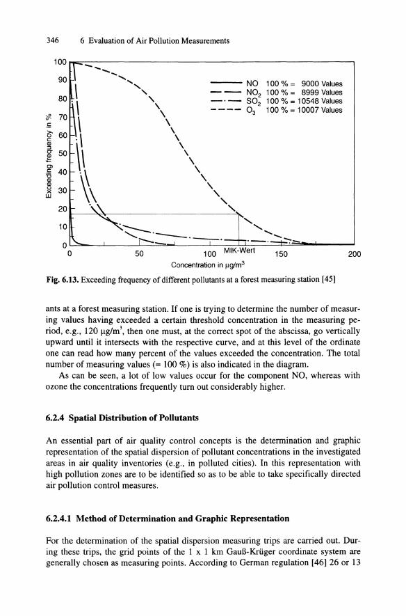
Fig. 6.13. Exceeding frequency of different pollutants at a forest measuring station [45]

ants at a forest measuring station. If one is trying to determine the number of measuring values having exceeded a certain threshold concentration in the measuring period, e.g., 120 flg/m3, then one must, at the correct spot of the abscissa, go vertically upward until it intersects with the respective curve, and at this level of the ordinate one can read how many percent of the values exceeded the concentration. The total number of measuring values (= 100 %) is also indicated in the diagram.

As can be seen, a lot of low values occur for the component NO, whereas with ozone the concentrations frequently turn out considerably higher.

6.2.4 Spatial Distribution of Pollutants

An essential part of air quality control concepts is the determination and graphic representation of the spatial dispersion of pollutant concentrations in the investigated areas in air quality inventories (e.g., in polluted cities). In this representation with high pollution zones are to be identified so as to be able to take specifically directed air pollution control measures.

6.2.4.1 Method of Determination and Graphic Representation

For the determination of the spatial dispersion measuring trips are carried out. During these trips, the grid points of the 1 x 1 km GauB-Kruger coordinate system are generally chosen as measuring points. According to German regulation [46] 26 or 13

z E Q)

E ~ :::l gj Q)

E '0 iii D E :::l Z


half-hourly measurements per year are preferably to be carried out, with 13 of them being the minimum. The area mean value II and the 98 % value 12 (short-term value) are formed from the measuring results of the 4 corners of a I x I km area. Thus, each area value is based on 104 or 52 (with 13 measurements per measuring point) half-hour values. The drawbacks of this determination method with so few measuring points per year will be discussed in more detail in the next section.

The reliability of the random measuring values can be improved by comparison with the results of continuously measured values which have been carried out simultaneously at a few points. The measuring values can turn out different from year to year depending on whether there were smog situations in the year of measurement or not and whether these were registered at some of the measuring points and not at others. In addition to the uncertainties of the random sample measuring method caused by the small number of measuring values, there is also the natural fluctuation of pollutant concentrations from year to year. Therefore, to determine the initial degree of pollution of the area to be surveyed, pollutant concentrations are to be determined by averaging the measuring values of at least three successive measuring periods (3 years) [46].

When setting up air quality inventories for air quality control concepts measurements are confined to a one-year duration, usually with only 26 measurements per measuring point, mostly due to reasons of expense.

Air quality inventories where pollutant concentrations are color-coded for each square kilometer can be found in numerous air quality control concepts [19, 22, 28-

1000

800

600

400

200

O~ ____ L-____ L-____ ~ __ ~

-100 -50 o 50 100 -100 -50 50 100 Uncertainty range d in % Uncertainty range d in %

Fig. 6.14. Uncertainty ranges of the mean value (a) and the 95 percentile (b) as a function of number of measurements N [50]


31]. It must be noted here, that these figures are mean area values of 1 km'. Depending on the presence of local pollutant sources there can be differences within these areas.

6.2.5 Methods for the Investigation of Consistent Patterns in the Occurrence of Pollutants

6.2.5.1 Mean Diurnal Courses

The calculation and graphic representation of mean diurnal courses are an appropriate means of identifying certain regularities in the occurrence of daily pollutant concentrations. For this, mean values are calculated for each half hour of the day from the data of the measuring period to be investigated and they are entered above the time of day. In this way the diurnal course of one average day is obtained.

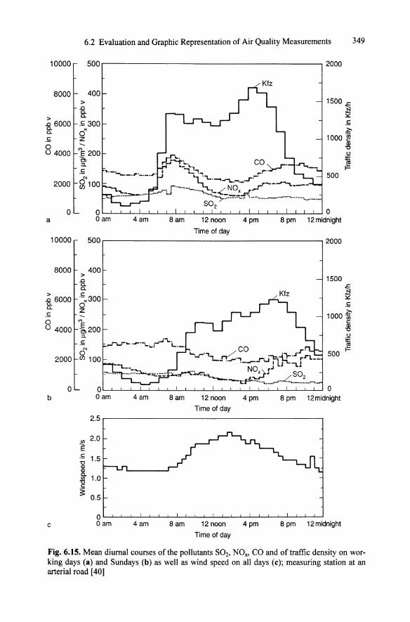
In streets with a lot of traffic pollution concentrations, e.g., depend on the traffic load on the one hand and on the atmospheric exchange conditions on the other. When representing mean diurnal courses the interrelationships become obvious. As the traffic load on Saturdays and Sundays is clearly different from the one on weekdays, it is advisable to represent the mean diurnal courses separately according to weekdays, Saturdays and Sundays. Fig. 6.15 shows that on weekdays the concentration maximum is distinctly higher in the morning (from 6:00 o'clock onwards) than in the afternoons, even though the traffic volume is greater in the afternoons. The influence of air exchange conditions which can be read off the mean diurnal course of the wind speed thus becomes obvious. In the morning, when the first rush hour is at its peak, the surface inversion is highly distinct and wind speed is at its minimum, which is why pollutant concentrations have their highest mean value then. With increasing wind speed in the further course of the day, pollutant concentrations decrease, even though the traffic load barely eases off. With the wind dropping in the afternoon, concentrations rise again. The widest maximum of concentrations is reached at a time when the traffic volume is already subsiding but the surface inversion is developing. At night the pollutants caused by traffic remain at a higher level than during the day because of the reduced change conditions over night. Two parameters, both of which influence the pollutant concentrations present,overlap here. If the cause of the pollution ceases to exist, e.g., the traffic maximum in the morning hours, then, despite inversion conditions, there is no concentration maximum of the polluting gases, as can be seen in the mean diurnal course of Sundays (Fig.6.15b). This course of events holds good for the majority of motor vehicle-related nitrogen oxides and carbon monoxide. With S02 the course of the heating activity, e.g., also forms part of the pollutant behavior.

The mean diurnal courses would be even more pronounced, if the days surveyed were grouped according to weather conditions, e.g., mean diurnal courses for weekdays with sunshine and nightly surface inversion on the one hand and days with overcast, windy weather on the other.

For the use of mean diurnal courses see also Figs. 3.19 and 3.23.

10000

8000

> '8. 6000 a. .5 0 t) 4000

2000

0 a

10000

8000

> '8. 6000 a. .5 0 t) 4000

2000

o b

c


500

400 >

.Q a. a. .5300 " 0

Z

ME 200 'C! :1. .5

0

,---------------------------------------,2000

1500 ~

~ .5 ~

1000 ~ ~

~ F

500

~~~~~~~~~~~~~~~~L_~~~~~O Oam 8 am 12 noon 4 pm 8 pm 12 midnight

Time of day 500 .-----------------------------------------.2000

400 > .c 1500 a. a. .5,,300 0

~ .5

Z >-...... M

1000 ~

~200 :1. .5

c -2! o ~

500 F

4am 8am 12 noon Time of day

4pm 8pm 12midnight

2.5.---------------------------------------,

U) 2.0 E .5 15 'C .

~ ~ 1.0 c ~ 0.5

O~~~-L~~~~_L~~~~~_L~~~~~~

Oam 4am Sam 12 noon Time of day

4pm S pm 12 midnight

Fig. 6.15. Mean diurnal courses of the pollutants S02. NOx• CO and of traffic density on working days (a) and Sundays (b) as well as wind speed on all days (c); measuring station at an arterial road [40]


6.2.5.2 Correlation Calculations

To establish the dependency of the occurring pollutant concentrations on other factors correlation calculations can be applied [57].

In forests, e.g., pollutant concentrations over the canopy and between the trees are determined by continuous measurements [45]. When the measuring values were assessed it was striking that concentration differences between the air above the canopy and the air within the trees were always particularly high when there was a high pollutant concentration up above. To examine the obvious dependencies more closely, all measuring values are entered in a diagram where the dependant variable parameter (in this case the concentration difference) is graphically represented over the independent variable parameter (in this case the pollutant concentration above the canopy). Fig. 6.16 shows two examples of this: the dependency of the concentration difference on those concentrations above the canopy of S02 and ozone. For the component S02 one can recognize a definite connection - all the values measured are positioned quite closely around the regression line and the calculated correlation coefficient is r2=0.998. The component OJ' however, is an example of a less obvious dependency. Here, sometimes high concentration differences occur even when pollutant concentrations above the canopy are low, and vice versa there are also small differences when there is a large amounty of ozone (r2=0.287). With ozone, chemical reactions which do not occur with S02 mask the dependency on the absolute pollutant concentration. Further information explaning pollutant behavior can be obtained from mean diurnal courses [45]. The dependencies shown here are not generally valid but only apply to the situation in the given measuring period at the measuring station mentioned.

In many cases it is advisable to investigate the dependencies of pollutant concentrations with the help of correlation calculations (further examples s. [45,58]).

6.2.5.3 Pollutant Wind Roses: Pollutant-Wind Correlations

In air quality measurements wind direction and wind speed should always be measured to find out from which direction atmospheric pollutants are transported to the measuring site. How representative of a larger or smaller area the measured wind directions are depends on the local topography, and must be checked in each individual case. In the diagram the measured wind directions (the most frequent values per each half hour respectively) can, e.g., be divided into 12 or 16 sectors and the frequency (in %) of the measuring values occurring in the individual sectors can be plotted in the circular coordinates. In this way the wind rose of the measuring period is obtained which can be divided according to wind speed sections, [45, 60).

If as in [35] every measured pollutant value is matched according to the wind direction (in 12 or 16 sectors), if the concentration's mean value is formed for each sector and if then these mean values are entered in the circular coordinates over the wind direction, then the so-called pollutant wind rose is obtained, s. Fig. 6.l7a, [45, 59]. If there are bulges in the concentration curve in certain sectors of the pollutant wind rose, then increased atmospheric pollutant concentrations are carried along with winds coming from these directions.


60.-----------~-----------,-----------.-----------,

" ",

.£

Correlation coefficient: 0.998 .: t-p":.' Regression line • ~ ~ ~ .. ;-",,1'"

~ • Pairs of values t::' g 40~------------~--------------~-------.~--~~~----------~ ~ Q) "C c: ~

~ ell

~ 20~------------~----~"~~--~--------------+-------------~ c: ~

~ o

N

o en

'" E C, ::i . £ ~ 0 c: ell 0

Q) "C c: ~

~ 0 .c ell <D 0 c: ~ ~ (5

'" 0

o

40

20

. o

20 40 60 80 802 Concentration above canopy in Ilg/m3

I I Correlation coefficient: 0.287

--- Regression line

• Pairs of values

. · . . . . . · . . . · . " . . · . .. . .. . · . t . · .. .''to . ,

' .. . . . .. . . . · . .. . . ; .. ~ . . # . . . . . ~ ..... .' ........ '" ..... .. . . ... .... ,.-. Ift"- ;.,. ~ .. ,\~ .. ~ .... .. .. r.:,. ~ :- ...... :'t . AM .... ....... .... --..... .. .. .. . : .. l; -4, .... A; .... ;& .. "~~."rM:: .. :t ...... "' .. w~';...:..a:-.-~ .... :.I... \.. r. .r.l(:" {~.~ •• ~J ~t .t...;.; ... ~ .... ~ .... r ... ~ .. ! ............

':f~~-"': t ·~G.f C .. \ ..... t .... A .. "" .......... .. .... AI

~~.... t~ .. t .. ~¥. '\I. .. ~ ... ~,t. ~ .. 1; ......... - - * .. ["Y!l1N....c4 ',' t • - .......... .. ,A ... :.( • .lot ~~~~ .. t~ At .... .. .............. r .... f· .. ·.,.~ .. ..... :"'....... .. I . ..

20 40 60 80 0 3 Concentration above canopy in Ilg/m3

Fig. 6.16. Dependency of concentration difference between the canopy (above the tree tops) and the interior forest on the concentration level above the canopy. Graphic representation and verification by correlation calculation. a: S02; b: 0 3 (lVD measuring stmion WaldenbuchBetzenberg, June 1986 [45])


N

SW

a S

N

SW

b S

SE

SE

E

NO. calms = 13.0 ~g/m3

N02• calms = 39.3 ~g/m3

Calms = 40.90 ~g/m3 N02

0.5 < WG < = 2.0 m/s 2.0 < WG < = 5.0 m/s

WG > 5.0 m/s


The following can be recognized from the pollutant wind rose shown in Fig. 6.17: the highest NO and N02 concentrations on the site of the measuring station (Schonbuch nature park) occur during winds from northerly directions. In this direction lies the greater Stuttgart area with its heavy traffic releasing nitrogen oxides which clearly pollute the Schonbuch nature park during northerly winds. In the mean, the lowest concentrations occur during southwesterly winds.

A slight increase in the nitrogen oxide wind rose occurs during southeasterly winds, implying sources in this direction.

Pollutant wind roses can also be drawn up for different wind speed classes. Fig. 6.17b shows a wind compass diagram divided into three wind speed classes [45]. It can be seen, that during week winds (0.5-2.0 mls) higher nitrogen oxide concentrations occur than during stronger winds (2.0-5.0 mls). During strong winds (> 5 mls) which solely come from southwesterly directions in this area, only very low nitrogen oxide concentrations occur.

The pollutant wind roses shown here do not provide information on the frequency of the concentrations determined in the individual sectors. It could, e.g., well be possible that the wind directions during which high concentrations were measured occurred only very rarely.

If the concentrations of the pollutant wind roses are multiplied by the corresponding frequency of the wind direction (affecting duration) and then divided by the total concentration mean value from all sectors, a pollutant dose wind rose is obtained. The values thus calculated provide information on which percentage contribution is made by a wind direction sector to the mean pollutant load at the measuring site. Detailed information on the representation of wind direction-related pollutant loads including examples of such pollutant dose wind roses is given in [60] by Baumiiller and Reuter.

One can also determine the total load by adding up all concentrations measured as half hourly mean values in the measuring period; also the concentrations of each wind direction sector can be added up and their contribution to the total load be determined. In this way, too, a pollutant dose wind rose is obtained representing the contribution of each wind direction to the total load. There is no difference between this pollutant dose wind rose and the one according to Baumiiller and Reuter relating to the mean value. The pollutant dose wind rose of Fig. 6.18 is based on the same measurements as those represented in Fig. 6.17. In this pollutant wind rose low concentrations, too, if they occur often enough contribute to the bulging of the dosage curve (e.g., direction southwest) owing to the high frequency of this wind direction. By comparison, the elevated concentrations measured during southeasterly winds (s. Fig. 6.17) occur so rarely that they practically do not show up in the dose wind rose.

Fig. 6.17. Pollutant wind roses; the pollutant mean values of the entire measuring period are represented in the individual wind direction sections; IVD forest measuring station in the Schonbuch (south of the greater Stuttgart area, FRG) [45]; measuring period: 11111986-31112/1986. B. NO and N02 mean values of all wind speeds; b. N02 mean values of different wind speed classes (WS)


N

SW

S

SE

NO, calms = 28.0 %

N02,calms = 19.9 %

Fig. 6.18. Pollutant dose wind rose; NO and N02 data of Fig. 6.17 at the IVD forest measuring station in the Sch5nbuch [45]; measuring period from 1I111986 to 12/3111986

Depending on the biological effectiveness of the pollutants the appropriate type of graphic representation must be chosen. If one is of the opinion that the frequent but very low concentrations do not have any effect, then the pollutant dose wind rose is certainly not a suitable means of representation as the low concentrations are overemphasized here by high wind direction frequencies. However, it would also be conceivable to draw a pollutant dose wind rose merely containing concentrations exceeding a certain threshold concentration. The criteria for this would have to be determined in cooperation with biologists and physicians. It must also be noted that pollutant concentration wind roses (Figs. 6.17a and b) do not lend themselves to short periods of measurement as individual sectors may only show with few measuring values which could be misleading. E.g., when evaluating just one month it is possible that, contrary to all theories, there are very high concentrations in some sectors. When checking this it can turn out that only one or two values caused this situation. A pollutant dose wind rose is better suited for short periods of measurement.

The German State Board for Air Quality Control in Essen applies another type of evaluation [61]: the flow density wind rose. It is formed by multiplying the pollutant concentrations in each sector with the wind speed prevailing at the time and by assessing them according to their frequency. In this way it is determined which pollut-


ant mass flows through an imaginary vertical surface of 1 m2 in one year at the measuring site. It must be emphasized that it is not a mass flow which is deposited on the ground or the vegetation. Apart from the frequency of the main wind direction the magnitude of the wind speed is included in this type of representation. As in Germany winds from westerly directions are the most frequent and also the strongest, these directions are strongly emphasized despite low concentrations.

It was shown that the representation of pollutant wind roses is an important means of determining the origin of atmospheric pollutants. However, even choosing a certain type of a pollutant wind rose can mean an interpretation of the measuring results in a certain way. One must therefore proceed with utmost care when applying and interpreting such wind direction-related representations.

6.2.5.4 Abatement Curves

It is often interesting to note how pollutant concentrations abate with increasing distance to the source, e.g., a street. Fig. 6.19 shows some abatement curves from measurements made on level terrain. When calculating these curves wind conditions may, of course, not be neglected. If, during the measurements, the wind blows against the street, then no traffic-related influence on measured concentrations can be detected even a short distance away (curve 4 in Fig. 6.19). On approximately level terrain the abatement curves usually have a profile like curves 2 and 3 [62]. The absolute level of the abating concentrations depends on the value of the initial concentrations, and these are again dependent on the source strength and on the weatherrelated exchange parameters. Curve 1 implies the abatement of the concentrations during low exchange weather conditions.

In street "canyons" (between rows of high buildings) atmospheric pollutants naturally behave differently [63]. Knowledge on abatement curves should have an effect on, e.g., development plans, suggesting residential areas near roads.

The dispersion of pollutants specific to motor vehicle traffic has been investigated in detail by Baumann [64] taking into account wind, time of day and street layout by using the example of a much frequented highway. Compared to a level roadway roads cutting below ground level are advantageous for the area in the immediate vicinity of the road at medium and high wind speeds; however, during weak wind conditions in general and low exchange weather conditions in particular, the load increases, as the air in the trough enriched with pollutants "overflows". This deep street bed layout of highways which can be found with increasing frequency represents a higher health hazard even for the road users themselves, as the motor vehicle emissions are channelled, cannot take part in the air exchange and thus accumulate.


100~~--,-----,-----,-----,-----,-----,

80 H--\-----'lct--

60

~ 0

.~ x

0 z

40

20~----~----+-----+-----4-----4-----4

O~--~----~----~----~----~----~

20 40 60 80 Distance in m

Fig. 6.19. Decreasing NOx concentration with increasing distance from an arterial road during different meteorological exchange conditions [40]. J surface inversion, wind speed <0.1 mis, wind contacting the highway at a small angle; 2 weak wind «I mls) at almost right angles to the highway, snowfall; 3 turbulent fair weather, wind speed - 2 mis, wind contacting the highway at a small angle; 4 turbulent fair weather, wind speed 2.5-3 mis, wind slanting towards the highway

6.3 Bibliography

1 VDI: Richtlinie 2450, BI. 1, Messen von Emission, Transmission und Immission luftverunreinigender Stoffe - Begriffe, Definitionen. Berlin: Beuth 9/1977

2 Stratmann, H.: Wirkungen von Luftverunreinigungen auf die Vegetation. LIS-Berichte Nr.49, Landesanstalt fUr Immissionsschutz, Essen 1984

3 Umweltbundesamt Bericht 9/80: Das Abgas-Emissionsverhalten von Personenkraftwagen in der Bundesrepublik Deutschland im Bezugsjahr 1980. TOV-Reinland im Auf trag des Umweltbundesamtes. Berlin: Erich Schmidt 1980

6.3 Bibliography 357

4 Umweltbundesamt Bericht 11/83: Das Abgas-Emissionsverhalten von Nutzfahrzeugen in der Bundesrepublik Deutschland im Bezugsjahr 1980. TOV-Rheinland im Auftrag des Urn weltbundesamtes. Berlin: Erich Schmidt 1983

5 Hauschulz, G.; Heich, HJ.; Leisen, P.; Raschke, J.; Waldeyer, H.; Winckler, J.: Emissions- und Immissionstechnik im Verkehrswesen. Kiiln: TOV Rheinland 1983

6 Meier, E.; PlaBmann, E.; Wolff, C. et a!.: Abgas-GroBversuch. AbschluBbericht, Vereinigung der Technischen Oberwachungsvereine e.V., Essen 1986

7 TOV Rheinland/Umweltbundesamt: Emissionsfaktoren fUr Luftverunreinigungen. Materialien 2/80. Berlin: Erich Schmidt 1980

8 Fiinfte Allgemeine Verwaltungsvorschrift zum Bundes-Immissionsschutzgesetz (Emissionskataster in Belastungsgebieten) - 5. BlmSch VwV yom 30.1.1979, GMB!., S. 42 f

9 Umweltbundesamt: Daten zur Umwelt 1986/87. Berlin: Erich Schmidt 1986 10 Dritte Verordnung zur DurchfUhrung des Bundes-Immissionsschutzgesetzes (Verordnung

iiber Schwefelgehalt von leichtem Heiziil und Dieselkraftstoff - 3. BImSch V) yom 15.1.1975, BGB!. I, S.264, geiindert durch Fassung yom 18.2.1986, BGB!. I, S.265 und durch Verordnung yom 14.12.1987, BGB!. I, S. 2 671f

11 Institut fUr wirtschaftliche Oelheizung e.V.: Die <Jlfeuerung, Ein Beitrag zur Reinhaltung der Luft. Druckschrift, Hamburg 1986

12 Chae, J.O.: Aufstellung eines mathematischen Modells der NOx-Bildung in eingeschlossenen turbulenten Erdgas-Diffusionsflammen. Dissertation Universitiit Stuttgart 1978

13 Schnell, U.: Die mathematische Modellierung der Stickstoffoxid-Emissionen von Kohlenstaubflammen. Diplomarbeit Nr.2204 am Institut fUr Verfahrenstechnik und Dampfkesselwesen der Universitiit Stuttgart 1986

14 Breuninger, H.A.; Baumbach, G.: Untersuchungen zur Wirksamkeit von Additiven fUr schweres Heizii!. Fortschr. Ber. VDI-Z. Reihe 6 Nr.113, 1983

15 Driischer, F.; Rauskolb, J.: Luftverunreinigungen in einem Schwarzwaldtal bei Inversionswetterlagen, Teil 2: Untersuchung der Staub-Immissionen. Institut fUr Verfahrenstechnik und Dampfkesselwesen der Universitiit Stuttgart, Abteilung Reinhaltung der Luft, Bericht Nr. 3, 1986

16 Ministerium fUr Erniihrung, Landwirtschaft, Umwelt und Forsten Baden-Wiirttemberg: Emissionskataster Stuttgart, Quellengruppe Verkehr. Stuttgart 1986

17 Ministerium fUr Erniihrung, Landwirtschaft, Umwelt und Forsten Baden-Wiirttemberg: Emissionskataster Mannheim, Quellengruppe Verkehr. Stuttgart 1986

18 Ministerium fiir Erniihrung, Landwirtschaft, Umwelt und Forsten Baden-Wiirttemberg: Emissionskataster Karlsruhe, Quellengruppe Verkehr. Stuttgart 1986

19 Baumbach, G.; Baumiiller, J.; Driischer, F.; Reuter, u.: Lufthygienisches Gutachten fUr die Stadt Heilbronn. Amt fUr StraBenverkehr und Umwelt, Heilbronn 1986

20 Ministerium fUr Erniihrung, Landwirtschaft, Umwelt und Forsten Baden-Wiirttemberg: Emissionskataster Stuttgart, Quellengruppe Hausbrand. Stuttgart 1986

21 Ministerium fUr Erniihrung, Landwirtschaft, Umwelt und Forsten Baden-Wiirttemberg: Emissionskataster Mannheim, Quellengruppe Hausbrand. Stuttgart 1986

22 Dreyhaupt, FJ.; Dierschke, W.; Kropp, K.; Prinz, B.; Schade, H.: Handbuch zur Aufstellung von Luftreinhaltepliinen. Kiiln: TOV Rheinland 1979

23 Baumbach, G.; Cannon, T.; Bauer, L.; Bisinger, R.: Luftqualitiit in Waldenbuch. Institut fUr Verfahrenstechnik und Dampfkesselwesen der Universitiit Stuttgart, Abt. Reinhaltung der Luft, Bericht Nr. 1 - 1985

24 Vierte Verordnung zur DurchfUhrung des Bundes-Immissionsschutzgesetzes (Verordnung iiber genehmigungsbediirftige Anlagen). 4. BImSchV yom 24.7.1985, BGB!. I, S.1586f

25 Elfte Verordnung zur DurchfUhrung des Bundes-Immissionsschutzgesetzes (Emissionserkliirungsverordnung). 11. BImSch V yom 20.12.1978, BGB!. I, S. 2027 f, geiindert durch Verordnung yom 14.7.1985, BGB!. I, S.1586 f

26 Ministerium fUr Erniihrung, Landwirtschaft, Umwelt und Forsten Baden-Wiirttemberg: Emissionskataster Stuttgart, Quellengruppe Industrie und Gewerbe. Stuttgart 1986

27 Ministerium fUr Erniihrung, Landwirtschaft, Umwelt und Forsten Baden-Wiirttemberg: Emissionskataster Karlsruhe, Quellengruppe Industrie und Gewerbe. Stuttgart 1986

28 Ministerium fiir Arbeit, Gesundheit und Soziales des Landes Nordrhein-Westfalen: Luftreinhalteplan Ruhrgebiet Ost - Dortmund - 1979 - 1983. Diisseldorf 1978


29 Ministerium fUr Arbeit, Gesundheit und Soziales des Landes Nordrhein-Westfalen: Luftreinhalteplan Rheinschiene-Sud - 1. Fortschreibung - 1982-1986. Dusseldorf 1984

30 Hessischer Minister fUr Landesentwicklung, Umwelt, Landwirtschaft und Forsten: Luftreinhalteplan Rhein-Main. Wiesbaden 1981

31 Ministerium fur Soziales, Gesundheit und Umwelt des Landes Rheinland Pfalz: Luftreinhalteplan Ludwigshafen/Frankenthal 1979 -1984. Mainz 1980

32 Kutzner, K.: Der Hausbrand als bodennahe Emissionsquelle - Fliichendeckende Emissionen und ihre Bedeutung fUr die Lufthygiene. VOl Ber. Nr. 477 "Reinhaltung der Luft in groBen Stiidten", Diisseldorf 1983

33 Friedrich, R.; Miiller, T.; Scheirle, N.; VoB, A.: Feinmaschiges Kataster der S02- und NO.Emissionen in Baden-Wurttemberg und im Oberrheintal - Emissionsuntersuchungen im Rahmen des TULLA-Projektes, in Bericht uber das 1. Statuskolloquium des PEF. S. 373 - 384, Kernforschungszentrum Karlsruhe 1985

34 Boysen, B.; Friedrich, R.; Muller, T.; Scheirle, N.; VoB, A.: Feinmaschiges Kataster der S02-und NO.-Emissionen in Baden-Wurttemberg fur die Zeit der TULLA-MeBkampagne, in Bericht uberdas 2. Statuskolloquium des PEF. Band 2, S. 481-492, Kernforschungszentrum Karlsruhe 1986

35 Vierte Allgemeine Verwaltungsvorschrift zum Bundes-Immissionsschutzgesetz (Ermittlung von Immissionen in Belastungsgebieten) vom 8.4.1975. GMBI. S.358

36 Baumbach, G.; Konrad, G.; Minner, G.: Luftverunreinigungen in einem Schwarzwaldtal bei Inversionswetterlagen, Teil 1. Institut fUr Verfahrenstechnik und Dampfkesselwesen der Universitiit Stuttgart, Abteilung Reinhaltung der Luft, Bericht Nr. 3 -1986

37 Umweltbundesamt: Monatsberichte aus dem MeBnetz. Sammelband 1983, Hrsg.: Umweltbundesamt, Fachgebiet II 6.3, Berlin 1984

38 Stem, A.C.; Boubel, R.W.; Furner, D.B.; Fox, D.L.: Fundamentals of Air Pollution. Orlando, Florida: Academic Press 1984

39 Verordnung der Landesregierung, des Ministeriums fUr Umwelt und des Innenministeriums zur Verhinderung schiidlicher Umwelteinwirkungen bei austauscharmen Wetterlagen (Smog-Verordnung-Smog YO) vom 27.6.1988. Gesetzblatt fUr Baden-Wurttemberg 1988, S.214f

40 Baumbach, G.: Derzeitige und zukunftige Schadgas-Immissionsbelastung an der B 10 in Stuttgart-Stammheim Sud. Gutachten fUr das Stadtplanungsamt Stuttgart 1981

41 Baumuller, J.; Hofmann, u.: Langjiihrige Schwefeldioxid-Messungen in Stuttgart 1965-1978. Chemisches Untersuchungsamt der Landeshauptstadt Stuttgart, Abt. Klimatologie, Mitteilung Nr.2, Stuttgart 1980

42 Landesanstalt fUr Umweltschutz Baden-Wurttemberg: Zweiter Umweltbericht Baden-Wiirttemberg 1983, Karlsruhe 1983

43 Baumuller, J.; Reuter, u.; Hoffmann, U.: Luftschadstoffe und Klima im Raum Stuttgart Vaihingen/Mohringen. Chemisches Untersuchungsamt der Landeshauptstadt Stuttgart, Abt. Klimatologie, Mitteilung Nr.9, Stuttgart 1985

44 Umweltbundesamt: Monatsberichte aus dem MeBnetz 2/84. Berlin 1984 45 Baumbach, G.; Baumann, K.; Droscher, F.: Luftverunreinigungen in Wiildern. Institut fur

Verfahrenstechnik und Dampfkesselwesen der Universitiit Stuttgart, Abt. Reinhaltung der Luft, Bericht Nr. 5 -1987

46 Erste allg. Verwaltungsvorschrift zum Bundes-Immissionsschutzgesetz (Technische Anleitung zur Reinhaltung der Luft - TA Luft) vom 27.2.1986. GMBI. S.95f

47 Statistische Berichte, Umwelt, Immissions-Konzentrationsmessungen. Hrsg. vom Statistischen Landesamt Baden-Wurttemberg, Stuttgart

48 KenngroBen der Ozonkonzentration fUr die UBA-MeBstellen, Monatsberichte aus dem MeBnetz, Februar 1983. Umweltbundesamt Berlin 1984

49 Landesanstalt fUr Immissionsschutz des Landes NRW: Monatsbericht uber die Luftqualitiit an Rhein und Ruhr 1/85. Essen 1985

50 Buck, M.; Doppelfeld, A.: Die Bedeutung des Stichprobenumfanges bei der Messung und Bewertung von Immissionen. Schriftenreihe der Landesanstalt fUr Immissionsschutz des Landes NRW, Verlag W. Giradet, Essen, H. 50 (1980) 31-40

51 Beier, R.: Zur Kennzeichnung von Immissionsbelastungen durch Quantile von Schadstoffverteilungen. Schriftenreihe der Landesanstalt fUr Immissionsschutz des Landes NRW, Verlag W. Giradet, Essen, H.55 (1982) 7-14

6.3 Bibliography 359

52 Beier, R.; Doppelfeld, A.: Statistische Analyse von Spitzenwerten stichprobenartig untersuchter Schadstoffkonzentrationen in der Aul3enluft. Schriftenreihe der Landesanstalt fUr Immissionsschutz des Landes NRW, Verlag W. Giradet, Essen, H.57 (1983) 7 -14

53 Junker, A.; Kiihner, D.: Mel3haufigkeit und Aussagesicherheit bei kontinuierlichen Immissionsmessungen. Staub-Rein halt. Luft 39 (1979) Nr.l, S.22-25

54 Miiller, H.G.: Statistische Methoden zur Beurteilung der Immissionsstruktur. 1m Auftrag des Umweltbundesamtes Berlin, Abschlul3bericht, Dornier System GmbH, Friedrichshafen 1977

55 VDI: VDI-Richtlinie 2310, B1.11, Maximale Immissions-Werte zum Schutze des Menschen (Schwefeldioxid). Berlin: Beuth 8/1984

56 Erste allg. Verwaltungsvorschrift zum Bundes-Immissionsschutzgesetz (Technische Anleitung zur Reinhaltung der Luft - TA Luft) vom 28.8.1974. GMBI A, 25 (1974) Nr.24, S.425-452

57 Kreyszig, E.: Statistische Methoden und ihre Anwendungen. Gottingen: Vandenhoeck & Ruprecht 1985

58 Baumbach, G.: Gleichzeitige Erfassung von Aul3enluft- und Innenraumkonzentrationen verschiedener Schadstoffe. VDI Ber. Nr. 608 (1987) 537 - 557

59 Baumbach, G.; Baumann, K.; Droscher, F.: Luftqualitat in Freudenstadt. Institut fiir Verfahrenstechnik und Dampfkesselwesen der Universitat Stuttgart, Abt. Reinhaltung der Luft, Bericht Nr. 6 - 1987

60 Baumiiller, J.; Reuter, u.: Hinweise zur Darstellung windrichtungsabhangiger Schadgasbelastungen. Staub-Reinhalt. Luft 44 (1984) Nr. 4, S. 183 -186

61 Pfeffer, H.U.: Immissionserhebungen in quellfernen Gebieten Nordrhein-Westfalens. StaubReinhalt. Luft 45 (1985) Nr. 6, S. 287 - 293

62 Esser, J.: Schadstoffkonzentrationen im Nahbereich von Autobahnen in Abhangigkeit von Verkehr und Meteorologie. In: Abgasbelastungen durch den Kraftfahrzeugverkehr. Koln: TOV Rheinland 1982, S. 165 - 183

63 Waldeyer, H.; Leisen, P.; Miiller, W.R.: Die Abhangigkeit der Immissionsbelastung in Stral3enschluchten von meteorologischen und verkehrsbedingten Einflul3grol3en. In: Abgasbelastungen durch den Kfz-Verkehr. Koln: TOV Rheinland 1982, S. 85 -114

64 Baumann, K.: Schadstoffausbreitung im Nahbereich einer Autobahn. Institut fUr Verfahrenstechnik und Dampfkesselwesen der Universitat Stuttgart, Abt. Reinhaltung der Luft, Bericht Nr. 8 - 1987

air quality control || evaluation of air pollution measurements

Documents