ACTIVE INVESTMENT STRATEGIES

Chapter 20

Bank ManagementBank Management, 5th edition.5th edition.Timothy W. Koch and S. Scott MacDonaldTimothy W. Koch and S. Scott MacDonaldCopyright © 2003 by South-Western, a division of Thomson Learning

Unlike loans and deposits, which have negotiated terms, bank investments generally represent impersonal financial instruments.

As such, portfolio managers can buy or sell securities at the margin to achieve aggregate risk and return objectives without the worry of adversely affecting long-term depositor or borrower relationships.

Investment strategies can subsequently play an integral role in meeting overall asset and liability management goals regarding interest rate risk, liquidity risk, credit risk, the bank’s tax position, expected net income, and capital adequacy.

Unfortunately, not all banks view their securities portfolio in light of these opportunities.

Many smaller banks passively manage their portfolios using simple buy and hold strategies.

The purported advantages are that such a policy requires limited investment expertise and virtually no management time, lowers transaction costs, and provides for predictable liquidity.

Regulators reinforce this approach by emphasizing the risk features of investments and not available returns. For example, the Comptroller’s Handbook states that

“the investment account is primarily a secondary reserve for liquidity rather than a vehicle to generate speculative profits. Speculation in marginal securities to generate more favorable yields is an unsound banking practice.”

The maturity or duration choicefor long-term securities

The optimal maturity or duration is possibly the most difficult choice facing portfolio managers.

It is very difficult to outperform the market when forecasting interest rates.

Some managers justify passive buy and hold strategies because of a lack of time and expertise.

Other managers actively trade securities in an attempt to earn above average returns.

Passive maturity strategies

Laddered (or staggered) maturity strategy management initially specifies a maximum

acceptable maturity and securities are evenly spaced throughout maturity

securities are held until maturity to earn the fixed returns

Barbell maturity strategy differentiates investments between those

purchased for liquidity and those for income short term securities are held for liquidity while

long term securities for income

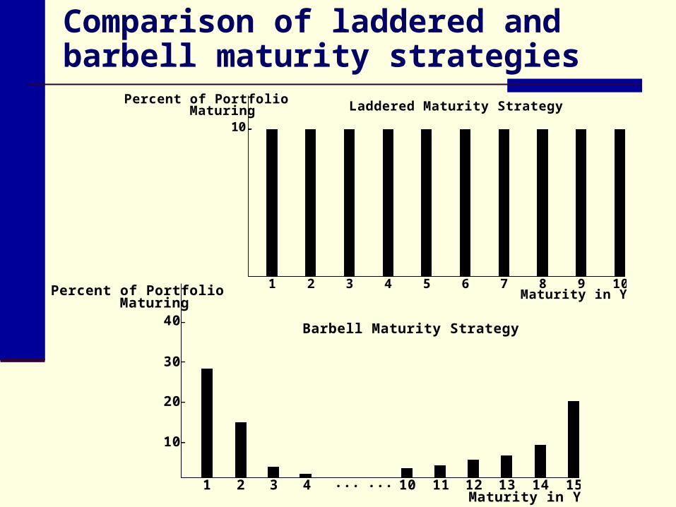
Comparison of laddered and barbell maturity strategies

Percent of PortfolioMaturing

10

1 2 3 4 5 6 7 8 9 10

Laddered Maturity Strategy

Maturity in YearsPercent of PortfolioMaturing

40

1 2 3 4 10 11 12 13 15

Barbell Maturity Strategy

30

20

10

... ... 14Maturity in Years

Active maturity strategies

Active portfolio management involves taking risks to improve total returns by adjusting maturities, swapping securities, and periodically liquidating discount instruments.

To be successful, the bank must avoid the trap of aggressively buying fixed-income securities at relatively low rates when loan demand is low and deposits are high.

Riding the yield curve

This strategy works best when the yield curve is upward-sloping and rates are stable.

There are three basic steps: identify the appropriate investment horizon buy a par value security with a maturity longer

than the investment horizon and where the coupon yield is higher in relationship to the overall yield curve

sell the security at the end of the holding period and time remains before maturity

Buy a 5-Year Security Buy a 10-Year Security and Sell It after 5 Years

Period: Year-End

Coupon Interest

Reinvestment Income at

7%

Coupon Interest

Reinvestment Income at

7% 1 $7,600 - $ 8,000 - 2 7,600 $ 532 8,000 $ 560 3 7,600 1,101 8,000 1,159 4 7,600 1,710 8,000 1,800 5 7,600 2,362 8,000 2,486

Total $38,000 $5,705 $40,000 $6,005 5 Principal at Maturity = $100,000 Price at Sale after 5 years = $101,615 when rate = 7.6%

Effect of riding the yield curve on total return when interest rates are stable

Initial conditions and assumptions: •5-year investment horizon

•yield curve is upward-sloping,

•5-year securities yielding 7.6 % and

•10-year securities yielding 8 %.

•Annual coupon interest is reinvested at 7%.

Expected Total Return Calculation

0.0752

1100,000

5,70538,000100,000i

1/5

5yr

0.0810

1100,000

6,00540,000101,615y

1/5

10yr

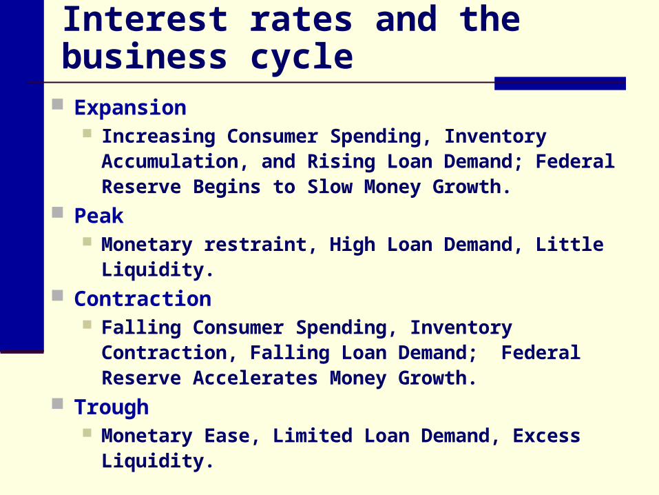
Interest rates and the business cycle

Expansion Increasing Consumer Spending, Inventory

Accumulation, and Rising Loan Demand; Federal Reserve Begins to Slow Money Growth.

Peak Monetary restraint, High Loan Demand, Little Liquidity.

Contraction Falling Consumer Spending, Inventory Contraction,

Falling Loan Demand; Federal Reserve Accelerates Money Growth.

Trough Monetary Ease, Limited Loan Demand, Excess

Liquidity.

Interest rates and the business cycle

The inverted U.S. yield curve has predicted these recessions:

Passive strategies over the business cycle.

One popular passive investment strategy follows from the traditional belief that a bank’s securities portfolio should consist of primary reserves and secondary reserves.

This view suggests that banks hold short-term, highly marketable securities primarily to meet unanticipated loan demand and deposit withdrawals. Once these primary liquidity reserves are established, banks invest

any residual funds in long-term securities that are less liquid but offer higher yields.

A problem arises because banks normally have excess liquidity during contractionary periods when consumer spending is low, loan demand is declining, unemployment is rising, and the Fed starts to pump reserves into the banking system. Interest rates are thus relatively low.

Banks employing this strategy add to their secondary reserve by buying long-term securities near the low point in the interest rate cycle. Long-term rates are typically above short-term rates, but all rates

are relatively low. With a buy and hold orientation, these banks lock themselves into

securities that depreciate in value as interest rates move higher.

Active strategies and the business cycle.

Many portfolio managers attempt to time major movements in the level of interest rates relative to the business cycle and adjust security maturities accordingly.

Some try to time interest rate peaks by following a contracyclical investment strategy defined by changes in loan demand.

The strategy entails both expanding the investment portfolio and lengthening maturities when loan demand is high, and alternatively contracting the portfolio and shortening maturities when loan demand is weak.

As such, the bank goes against the credit (lending) cycle. Note that the yield curve generally inverts when

rates are at their peak prior to a recession.

Issues for securities with embedded options

Callable agency securities or mortgage-backed securities have embedded options.

To value a security with an embedded option, three questions must be addressed: Is the investor the buyer or seller of the

option? How and by what amount is the buyer being

compensated for selling the option, or how much must it pay to buy the option?

When will the option be exercised and what is the likelihood of exercise?

Price-yield relationship for securities with embedded options

5.78%

3-Year, $100 Par Value FHLB Bond, Callable afterOne Year, Priced at $99.97

Yield

A. Callable Agency Bond

Pri

ce

100

$99.97

7% 9.5%Yield onMortgages

B. High-Coupon, Interest-Only Mortgage-Backed Security

Pri

ce

of

IO

P*

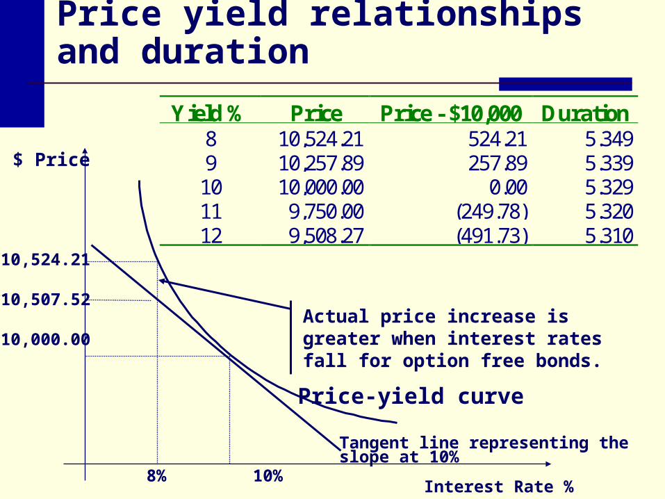
Price yield relationships and duration

Yield % Price Price - $10,000 Duration8 10,524.21 524.21 5.3499 10,257.89 257.89 5.339

10 10,000.00 0.00 5.32911 9,750.00 (249.78) 5.32012 9,508.27 (491.73) 5.310

$ Price

Actual price increase is greater when interest rates fall for option free bonds.

10,524.21

10,507.52

10,000.00

8% 10%Interest Rate %

Price-yield curve

Tangent line representing the slope at 10%

Δi

%ΔΔ

i+1ΔiP

ΔP

DUR

Duration is an approximate measure of the price elasticity of demand

Solve for Price: P - Duration x [ i / (1 + i)] x P

Price (value) changes Longer maturity/duration larger changes in

price for a given change in i-rates Larger coupon smaller change in price for a

given change in i-rates

The relationship between duration and actual changes in securities prices

The difference between the actual price-yield curve and the straight line representing duration at the point of tangency equals the error in applying duration to estimate the change in bond price at each new yield.

For both rate increases and rate decreases, the estimated price, based on duration, will be below the actual price. For small changes in yield, such as yields near 10

percent, the error is small. For large changes in yield, such as yields well

above or well below 10 percent, the error is large.

Duration and convexity

The relationship between price and interest rates is not the same for any change in interest rates.

Duration will generally be a ‘good’ estimate of price volatility only for very small changes in interest rates.

The greater the change in interest rates, the less accurate duration will be as a measure of price volatility.

Convexity

Convexity is a measure of the rate of change of dollar duration as yields change.

Duration, increases as yields decline and lengthens as yields increase for all option free bonds. This is positive feature for buyers of bonds because as

yields decline, price appreciation accelerates. As yields increase, duration for option free bonds

decreases, once again reducing the rate at which price declines.

This characteristic is called positive convexity-- the underlying bond becomes more price sensitive when yields decline and less price sensitive when yields increase.

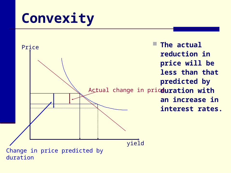
Convexity

The actual reduction in price will be less than that predicted by duration with an increase in interest rates.

Change in price predicted by durationyield

Price

Actual change in price

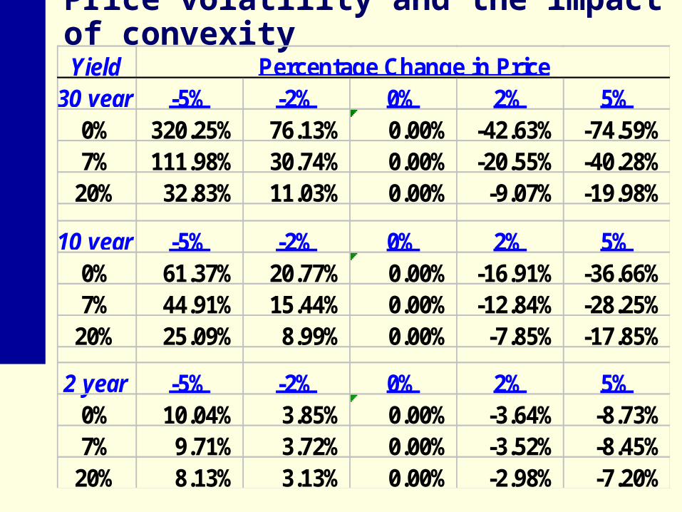
Price volatility and the impact of convexityYield

30 year -5% -2% 0% 2% 5%0% 320.25% 76.13% 0.00% -42.63% -74.59%7% 111.98% 30.74% 0.00% -20.55% -40.28%

20% 32.83% 11.03% 0.00% -9.07% -19.98%

10 year -5% -2% 0% 2% 5%0% 61.37% 20.77% 0.00% -16.91% -36.66%7% 44.91% 15.44% 0.00% -12.84% -28.25%

20% 25.09% 8.99% 0.00% -7.85% -17.85%

2 year -5% -2% 0% 2% 5%0% 10.04% 3.85% 0.00% -3.64% -8.73%7% 9.71% 3.72% 0.00% -3.52% -8.45%

20% 8.13% 3.13% 0.00% -2.98% -7.20%

Percentage Change in Price

The impact of prepayments on duration and yield for bonds with options

In general, market participants price mortgage-backed securities by following a 3-step procedure: estimate duration based on an assumed

interest rate environment and prepayment speed

identify a zero-coupon Treasury security with the same (approximate) duration.

the MBS is priced at a mark-up over the Treasury.

The MBS yield is set equal to the yield on the same duration Treasury plus a spread. The spread can range from 50 to 300 basis

points depending on market conditions. The MBS yields reflect the zero-coupon

Treasury yield curve plus a premium.

Impacts of prepayments on modified duration and price of a GNMA pass-through security

G N S F 7 1 / 2 7 . 5 %

3/ 1/99 Y I E L D T A B L E

Generic: GNMA I

next pay 4/15/99 (monthly)rcd date 3/31/99 (14 Delay)accrual 3/ 1/99 - 3/31/99

AgeWAM*WAC*

128

84

8.00

GNSF 7.5 A 8.000 (340) 20 WAC (UAM) CAGE

Obp 258 +300bp 94 +200bp 113 +100bp 152 -100bp 602 -200bp 817 -300bp 921

1mo3mo6mo

12moLife

B: Median :

VaryPRICE

132

102-11102-13102-15102-17102-19102-21102-23AvgLifeMod Dur

6.9586.9436.9276.9126.8976.8826.8675.574.01

7.2147.2057.1967.1867.1777.1687.158

11.126.54

7.1877.1777.1677.1577.1477.1377.127

10.106.12

7.1287.1177.1057.0947.0837.0717.0608.425.39

6.3266.2966.2666.2366.2076.1776.1472.392.05

5.8665.8265.7865.7455.7055.6655.6251.681.51

5.6225.5765.5305.4845.4385.3925.3461.451.33

2. 258 PSA 94 PSA 113 PSA 152 PSA 602 PSA 817 PSA 921 PSA

592.P587671524203

30.7C35.431.726.613.3

GG

<GD>

::

WAC - weighted average coupon WAM -

weighted average maturity

Effective duration and effective convexity

Effective duration and effective convexity are used to estimate a securities price sensitivity when the security contains embedded options.

)i (iP

P-P duration Effective

-0

i-i

where Pi- = price if rates fall, Pi+ = price if rates rise; P0 = initial (current) price;P* = initial price

2-i-i

)]i [0.5(i*P

*2PPP convexity Effective

i+ =initial market rate plus the increase in rate; i- = initial market rate minus the decrease in rate

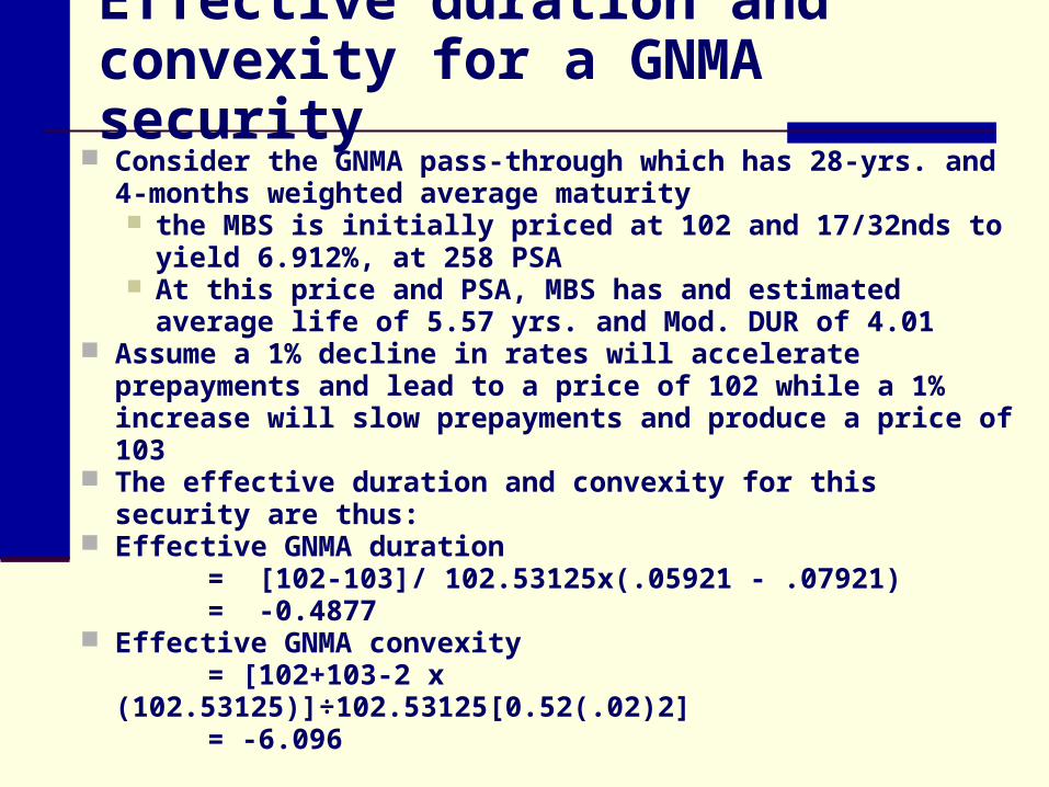
Effective duration and convexity for a GNMA security

Consider the GNMA pass-through which has 28-yrs. and 4-months weighted average maturity the MBS is initially priced at 102 and 17/32nds to yield

6.912%, at 258 PSA At this price and PSA, MBS has and estimated average

life of 5.57 yrs. and Mod. DUR of 4.01 Assume a 1% decline in rates will accelerate prepayments

and lead to a price of 102 while a 1% increase will slow prepayments and produce a price of 103

The effective duration and convexity for this security are thus:

Effective GNMA duration = [102-103]/ 102.53125x(.05921 - .07921) = -0.4877

Effective GNMA convexity = [102+103-2 x (102.53125)]÷102.53125[0.52(.02)2]= -6.096

Positive and negative convexity

Option-free securities exhibit positive convexity because as rates increase, the percentage price decline is less than the percentage price increase associated with the same rate decline.

Securities with embedded options may exhibit negative convexity -- the percentage price increase is less than the percentage price decrease for equal negative and positive changes in rates.

Total return analysis …An investor’s actual realized return should reflect the coupon interest, reinvestment income, and value of the security at maturity or sale at the end of the holding period.

When a security carries embedded options, such as the prepayment option with mortgage-backed securities, these component cash flows will vary in different interest rate environments.

For example, if rates fall and borrowers prepay faster than originally expected, coupon interest will fall as the outstanding principal falls, reinvestment income will fall because rates are lower when the proceeds are reinvested and less coupon interest is received, and the price at sale (end of the holding period) may rise or fall depending on the speed of prepayments.

When rates rise, borrowers prepay slower so that coupon income increases, reinvestment income increases, and the price at sale (end of the holding period) again may rise or fall.

Total return analysis for a callable FHLB Bond

Total return analysis for a callable FHLB Bond

Option-adjusted spread

Standard calculation of yield to maturity is inappropriate with prepayment risk.

Option-adjusted spread (OAS) accounts for factors that potentially affect the likelihood and frequency of call and prepayments.

Static spread is the yield premium, in percent, that (when added to Treasury zero coupon spot rates along the yield curve) equates the present value of the estimated cash flows for the security with options equal to the prevailing price of the matched-maturity Treasury.

OAS represents the incremental yield earned by investors from a security with options over the Treasury spot curve, after accounting for when and at what price the embedded options will be exercised.

OAS analysis is one procedure to estimate how much an investor is being compensated for selling an option to the issuer of a security with options.

The approach starts with estimating Treasury spot rates (zero coupon Treasury rates) using a probability distribution and Monte Carlo simulation, identifying a large number of possible interest rate scenarios over the time period that the security’s cash flows will appear.

The analysis then assigns probabilities to various cash flows based on the different interest rate scenarios. For mortgages, one needs a prepayment model

and for callable bonds, one needs rules and prices indicating when the bonds will be called and at what values.

OAS analysis involves three basic calculations

1. For each scenario, a yield premium is added to the Treasury spot rate (matched maturity zero coupon Treasury rate) and used to discount the cash flows.

2. For every interest rate scenario, the average present value of the security’s cash flows is calculated.

3. The yield premium that equates the average present value of the cash flows from the security with options to the prevailing price of the security without options is the OAS.

Conceptually, OAS represents the incremental yield earned by investors from a security with options over the Treasury spot curve, after accounting for when and at what price the embedded options will be exercised.

Ste

ps in

op

tion

-ad

juste

d s

pre

ad

calc

ula

tion

Current Treasury Curve (Mean)

Distribution of Interest Rates

Rate Volatility Estimates (Variance)

Prepayment Model

Find Spread Over Treasury Rates Such That Market Price = Present Value of Cash Flows

Option-Adjusted Spread

Calculate Duration and Convexity

Shock Rates Up and Down

Market Price of Mortgage Security

Security-Specific Information: Coupon Rate, Maturity, etc.

Other Prepayment Factors

Possible Cash Flows form Mortgage Security

Option-adjusted spread analysis for a callable FHLB bond

Comparative yields on taxable versus tax-exempt securities

A bank’s effective return from investing in securities depends: on the amount of interest income, reinvestment income, potential capital gains or losses, whether the income is tax-exempt or taxable,

and whether the issuer defaults on interest and

principal payments. When making investment decisions, portfolio

managers compare expected risk-adjusted after-tax returns from alternative investments. they purchases securities that provide the

highest expected risk-adjusted return

Why are municipal securities so attractive to banks?

Most municipal securities are federal income tax exempt.

Suppose that you could borrow funds at 6%, deduct your interest expense at a 34% tax rate, and buy securities that pay tax-exempt interest at 5.75%.

Your before tax spread would be negative 0.25% but your after tax spread would be 1.79% after tax spread = 5.75% - [6% x (1 - 0.34)]

= 1.79% Ignoring credit and interest rate risk issues, you

would effectively pay 3.96% on borrowings:= 6% x (1 – 0.34)

After-tax and tax-equivalent yields

Once the investor has determined the appropriate maturity and risk security, the investment decision involves selecting the security with the highest after-tax yield.

Tax-exempt and taxable securities can be compared as:

t)(1RR tm

whereRm = pretax yield on a municipal securityRt = pretax yield on a taxable securityt = investor’s marginal federal income tax rate

Example: After tax returns

Let:Rm = 5.75%Rt = 7.50% bank's average cost of funds = 6.00%marginal tax rate = 34%

The investor would choose the municipal because it pays a higher after tax return:

Rm = 5.75% after taxes

Rt = 7.50% (1 - 0.34) = 4.95% after taxes

Marginal tax rates implied in the taxable - tax-exempt spread.

If taxable securities (Corp.) and tax-exempt securities (Muni's) are the same for all other reasons then: t* = 1 - (Rm / Rt) where

Rm = pretax yield on a municipal security Rt = pretax yield on a taxable security

t* represents the marginal tax rate at which an investor would be indifferent between a taxable and a tax-exempt security equal for all other reasons.

Higher marginal tax rates or high tax individuals (companies) will prefer tax-exempt securities.

Example: Implied marginal tax rate

Let:Rm = 5.75%Rt = 7.50% bank's average cost of funds = 6.00%marginal tax rate = 34%

An Investor would be indifferent between these two investment alternatives if her marginal tax rate were 23.33%

Municipals and state and local taxes

The analysis is complicated somewhat when state and local taxes apply to municipal securities:

Many analysts compare securities on a pre-tax basis

To compare municipals on a tax equivalent basis (pre-tax):

)]t(t[1R)t(tR mtmm

t)(t1

)t(tR yieldequivalenttax

m

mm

Deductibility of interest expense

Prior to 1983, banks could deduct the full amount of interest paid on liabilities used to finance the purchase of muni's.

After 1983; however, 15% was not deductible and after 1984 20% was not deductible.

The 1986 tax reform act made 100% not deductible except for qualified muni's, small issue (less than 10 million).

The loss of interest expense deductibility will, in effect, be like an implicit tax on the bank's holding of municipal securities.

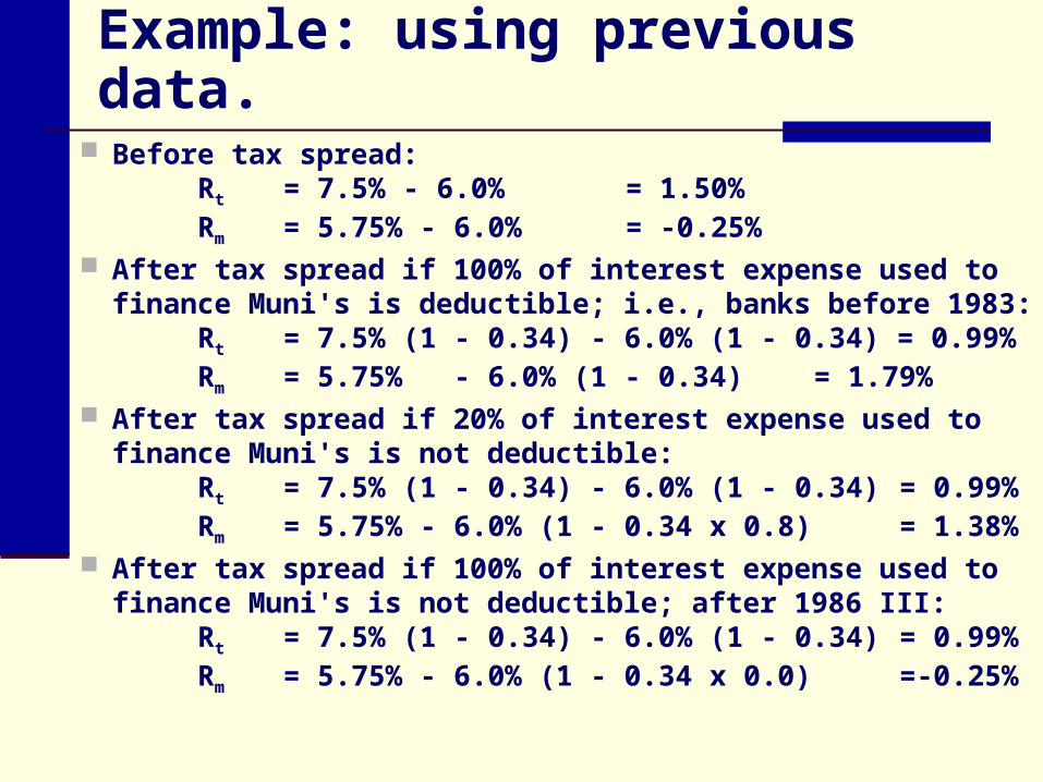
Example: using previous data.

Before tax spread:Rt = 7.5% - 6.0% = 1.50%Rm = 5.75% - 6.0% = -0.25%

After tax spread if 100% of interest expense used to finance Muni's is deductible; i.e., banks before 1983:

Rt = 7.5% (1 - 0.34) - 6.0% (1 - 0.34) = 0.99%Rm = 5.75% - 6.0% (1 - 0.34) = 1.79%

After tax spread if 20% of interest expense used to finance Muni's is not deductible:

Rt = 7.5% (1 - 0.34) - 6.0% (1 - 0.34) = 0.99%Rm = 5.75% - 6.0% (1 - 0.34 x 0.8) = 1.38%

After tax spread if 100% of interest expense used to finance Muni's is not deductible; after 1986 III:

Rt = 7.5% (1 - 0.34) - 6.0% (1 - 0.34) = 0.99%Rm = 5.75% - 6.0% (1 - 0.34 x 0.0) =-0.25%

Interest deductibility

Lost deductibility of interest expense is somewhat equivalent to an implied tax on municipal income.

To calculate after tax yields on muni's, if interest expense is not fully deductible, calculate the banks effective tax rate on municipals:

local and stateR

cost

interest

Pooled

Deductable

%nott

tmuni

m

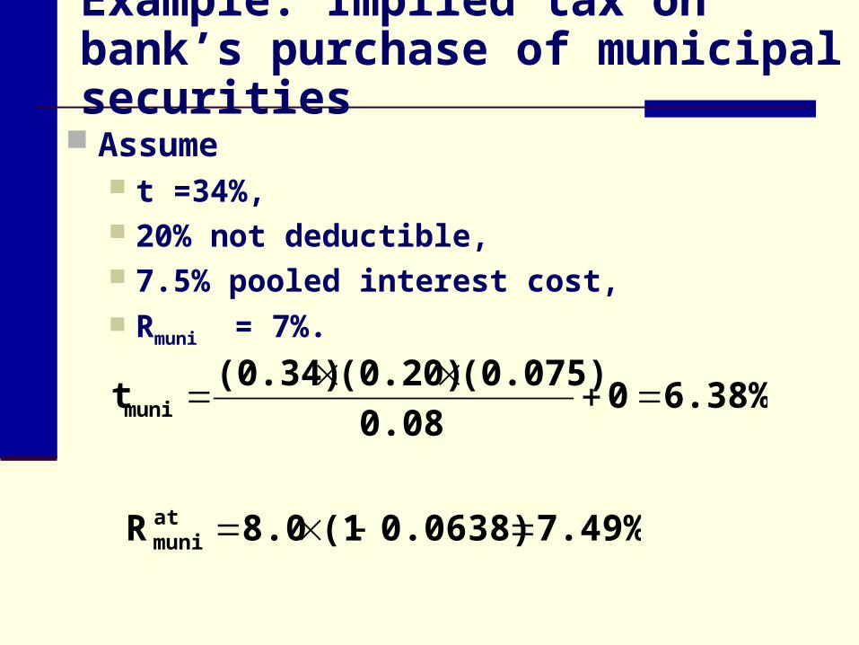
Example: Implied tax on bank’s purchase of municipal securities

Assume t =34%, 20% not deductible, 7.5% pooled interest cost, Rmuni = 7%.

7.49%0.0638)(18.0Ratmuni

6.38%00.08

(0.075)(0.20)(0.34)tmuni

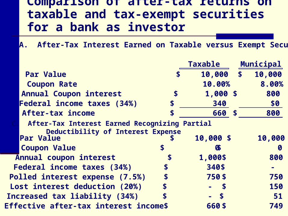
Comparison of after-tax returns on taxable and tax-exempt securities for a bank as investor

C. After-Tax Interest Earned Recognizing Partial Deductibility of Interest Expense

A. After-Tax Interest Earned on Taxable versus Exempt Securities

Taxable MunicipalPar Value 10,000$ 10,000$ Coupon Rate 10.00% 8.00%Annual Coupon interest 1,000$ 800$ Federal income taxes (34%) 340$ $0After-tax income 660$ 800$

Par Value 10,000$ 10,000$ Coupon Value 0$ 0$ Annual coupon interest 1,000$ 800$ Federal income taxes (34%) 340$ -$ Polled interest expense (7.5%) 750$ 750$ Lost interest deduction (20%) -$ 150$ Increased tax liability (34%) -$ 51$ Effective after-tax interest income 660$ 749$

After-tax interest earned, recognizing partial deductibility of interest expense: Individual asset

Factors affecting allowable deduction:

Total interest expense paid 1,500,000$

Average amount of assets owned 20,000,000$

Average amount of tax exempt securities owned: 800,000$

Weighted average cost of financing 7.50%

Nondeductible interest expense:

Pro rata share of interest expense to carry muni's 4.00%

Nondeductible interest expense (20%) 12,000$

Deductible interest expense: $1,500,000 - $12,000 = 1,488,000$

The impact of the tax reform act of 1986 (TRA 1986)

The TRA of 1986 created two classes of municipals:

1. Qualified and

2. Nonqualified Municipals After 1986, banks can no longer deduct

interest expenses associated with municipal investments, except for qualified municipal issues.

Qualified versus nonqualified municipals

Qualified Municipals banks can still deduct 80 percent of the

interest expense associated with the purchase of certain small issue public-purpose bonds.

Nonqualified Municipals all municipals that do not meet the qualified

criteria. Municipals issued before August 7, 1986,

retain their tax exemption; i.e., can still deduct 80 percent of their associated financing costs (grandfathered in).

Example: Implied tax on bank’s purchase of nonqualified municipal securities (100% lost deduction)

Assume t =34%, 20% not deductible, 7.5% pooled interest cost, Rmuni = 7%.

%45.5)3188.01(0.8R atmuni

%88.31008.0

)075.0()00.1()34.0(tmuni

Strategies underlying security swaps

Active portfolio strategies also enable banks to sell securities prior to maturity whenever economic conditions dictate that returns can be earned without a significant increase in risk.

When a bank sells a security at a loss prior to maturity, because interest rates have increased, the loss is a deductible expense.

At least a portion of the capital loss is reduced by the tax-deductibility of the loss.

Evaluation of security swaps

Par ValueMarket Value

RemainMaturity

SemiannCoupon YTM

A. Classic Swap DescriptionSell US Trea bonds @ 10.50% $2,000,000 $1,926,240 3 $105,000 12.00%Buy FHLMC bons @ 12.20% $1,952,056 $1,952,056 3 $119,075 12.20%

B. Swap with Minimal Tax EffectsSell US Treas bons @ 10.50% $2,000,000 $1,926,240 3 $105,000 12.00%Sell FNMA @ 13.80% $3,000,000 $3,073,065 4 $207,000 13.00% Total $5,000,000 $4,999,305 $312,000Buy FNMA @ 13.00% $5,000,000 $5,000,000 1 $325,000 12.00%

13,000$ C. Present Value AnalysisPeriod 0 1 2 3 4 5 6Treas Cash flow $1,926,240 ($105,000) ($105,000) ($105,000) ($105,000) ($105,000) ($2,105,000)Tax savings $25,816FHLMC ($1,952,056) $119,075 $119,075 $119,075 $119,075 $119,075 $2,071,132Difference: $0 $14,075 $14,075 $14,075 $14,075 $14,075 ($33,868)

$35,3801.061

14,07547,944

1.061

14,075PV

6

6

1tt

Security swap example

Tax Savings: = (2,000,000 - 1,926,240) * 0.35 = 25,816

After Tax Proceeds = 1,926,240 + 25,816 = 1,952,056

Present Value of the Difference:

$35,3801.061

14,07547,944

1.061

14,075PV

6

6

1tt

In general, banks can effectively improve their portfolios by

Upgrading bond credit quality by shifting into high-grade instruments when quality yield spreads are low

Lengthening maturities when yields are expected to level off or decline

Obtaining greater call protection when management expects rates to fall

Improving diversification when management expects economic conditions to deteriorate

Generally increasing current yields by taking advantage of the tax savings

Shifting into taxable securities from municipals when management expects losses

Leveraged arbitrage strategy

During the mid- to late-1990s, many bank managers believed that their banks were under-leveraged. Too little debt relative to stockholders’ equity lowered

the equity multiplier and reduced ROE, given the strong ROAs that were being generated.

To increase earnings and make the bank more expensive if an acquirer was interested in buying the bank, some portfolio managers implemented a leveraged arbitrage strategy involving borrowing from the Federal Home Loan Bank and using the proceeds to buy securities.

The specific strategy consists of matching the maturity of FHLB advances with the call dates of callable agency bonds and the maturity dates of securities currently held in the investment portfolio.

Example: Leveraged arbitrage strategy

Consider a bank with $100 million in assets and $12 million in stockholders’ equity that expects to earn $1.5 million, or 1.5 percent on assets.

The bank would report an equity multiplier of 8.33 and an ROE of 12.5%. The bank owns $3 million of Treasury securities @ 5.4% that mature in

one year, and $3 million in Farm Credit Bank bonds@ 5.7% that mature in 18 months.

It can borrow from the FHLB for one year at 6 percent and for 18 months at 6.2%.

The leveraged arbitrage strategy involves borrowing from the FHLB at these maturities and buying callable agency bonds with call dates at one year and 18 months, respectively.

For example, assume that a 5-year maturity bond, noncallable for one year, yields 7 percent, while a 7-year bond that is noncallable for 18 months yields 7.25 percent. The spread between the respective advances and callable agencies is

Agency Interest FHLB Advance Interest Spread 5 NC 1 year 7% 6% 1% 7 NC 18 mo. 7.25% 6.2% 1.05%

If the transactions amounts were the same $3 million, the bank would earn an additional $61,500 in net interest income over the year.

This would lower the bank’s ROA to 1.45 percent, but increase the bank’s ROE to 12.84 percent.

ACTIVE INVESTMENT STRATEGIES

Chapter 20

Bank ManagementBank Management, 5th edition.5th edition.Timothy W. Koch and S. Scott MacDonaldTimothy W. Koch and S. Scott MacDonaldCopyright © 2003 by South-Western, a division of Thomson Learning