THE DETERMINATES OF INTEREST RATES

Chapter 7

Bank ManagementBank Management, 5th edition.5th edition.Timothy W. Koch and S. Scott MacDonaldTimothy W. Koch and S. Scott MacDonaldCopyright © 2003 by South-Western, a division of Thomson Learning

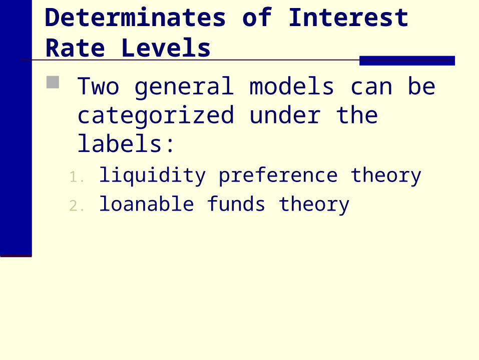
Determinates of Interest Rate Levels

Two general models can be categorized under the labels:

1. liquidity preference theory

2. loanable funds theory

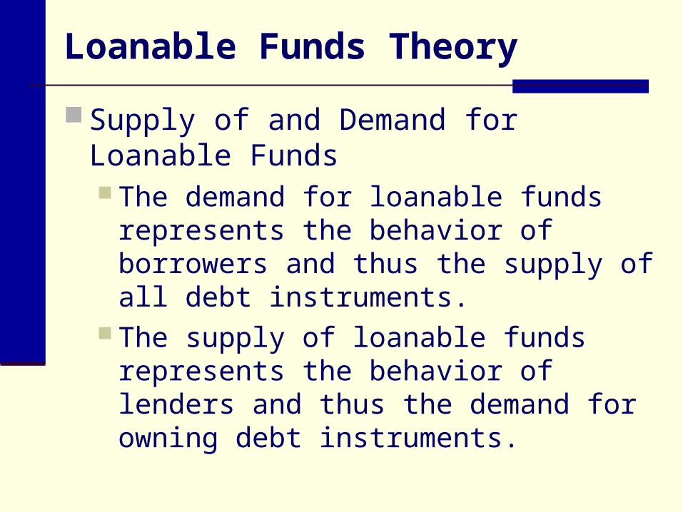
Loanable Funds Theory

Supply of and Demand for Loanable Funds The demand for loanable funds

represents the behavior of borrowers and thus the supply of all debt instruments.

The supply of loanable funds represents the behavior of lenders and thus the demand for owning debt instruments.

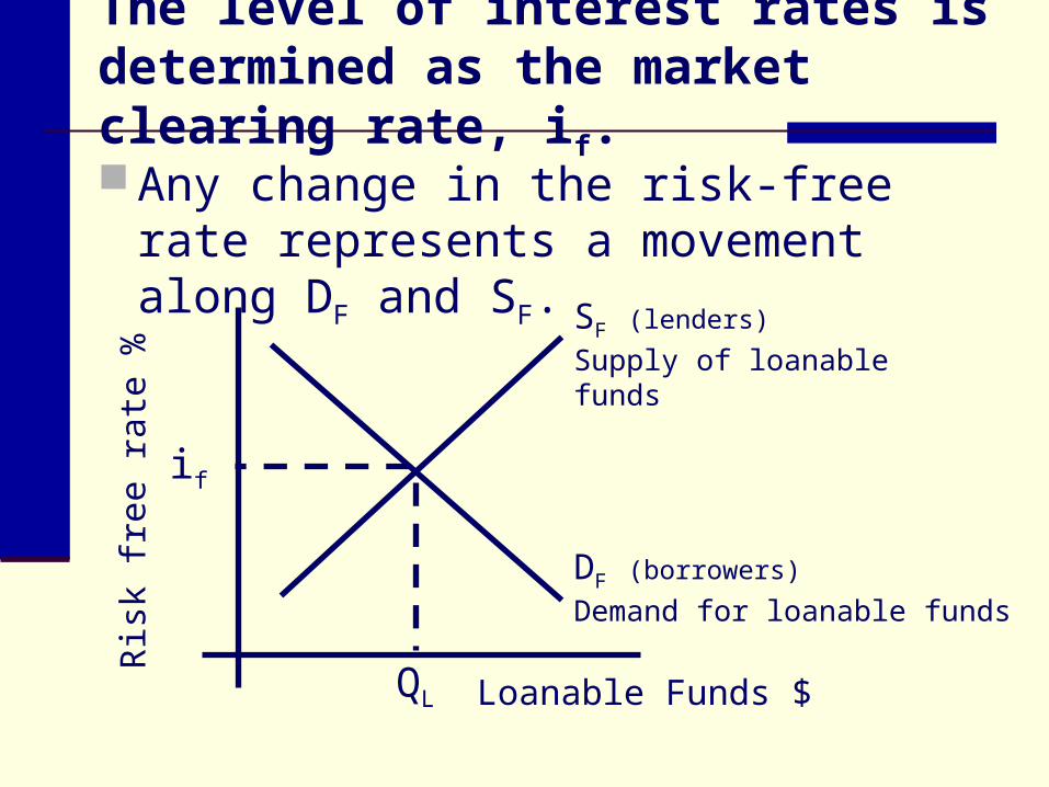
The level of interest rates is determined as the market clearing rate, if.

Any change in the risk-free rate represents a movement along DF and SF.

SF (lenders)

Supply of loanable funds

DF (borrowers)

Demand for loanable funds

Loanable Funds $

Ris

k fr

ee r

ate

%

if

QL

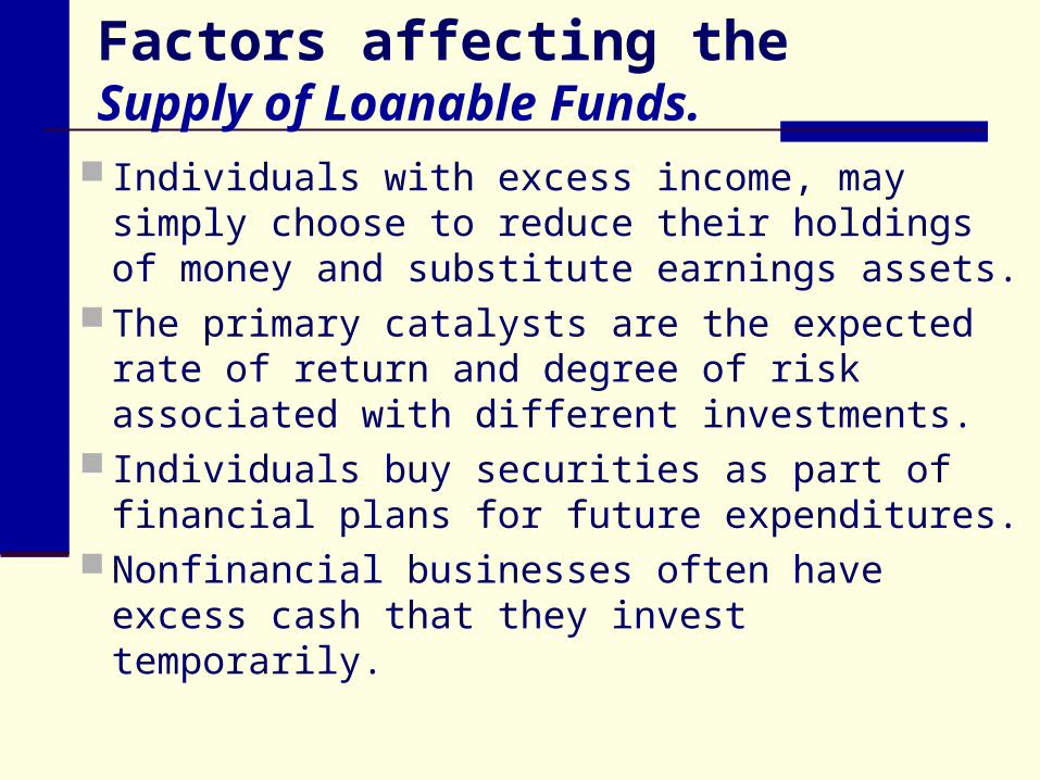
Factors affecting the Supply of Loanable Funds.

Individuals with excess income, may simply choose to reduce their holdings of money and substitute earnings assets.

The primary catalysts are the expected rate of return and degree of risk associated with different investments.

Individuals buy securities as part of financial plans for future expenditures.

Nonfinancial businesses often have excess cash that they invest temporarily.

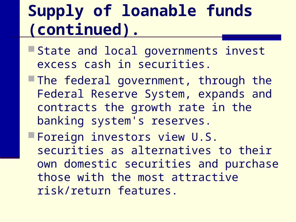
Supply of loanable funds (continued).

State and local governments invest excess cash in securities.

The federal government, through the Federal Reserve System, expands and contracts the growth rate in the banking system's reserves.

Foreign investors view U.S. securities as alternatives to their own domestic securities and purchase those with the most attractive risk/return features.

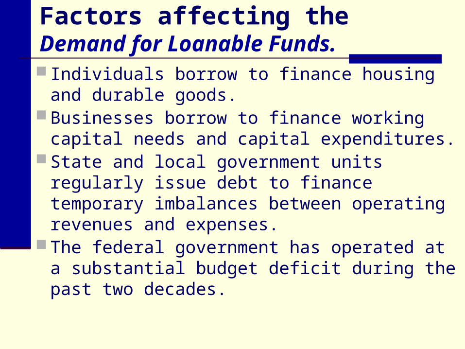
Factors affecting theDemand for Loanable Funds. Individuals borrow to finance housing and

durable goods. Businesses borrow to finance working capital

needs and capital expenditures. State and local government units regularly

issue debt to finance temporary imbalances between operating revenues and expenses.

The federal government has operated at a substantial budget deficit during the past two decades.

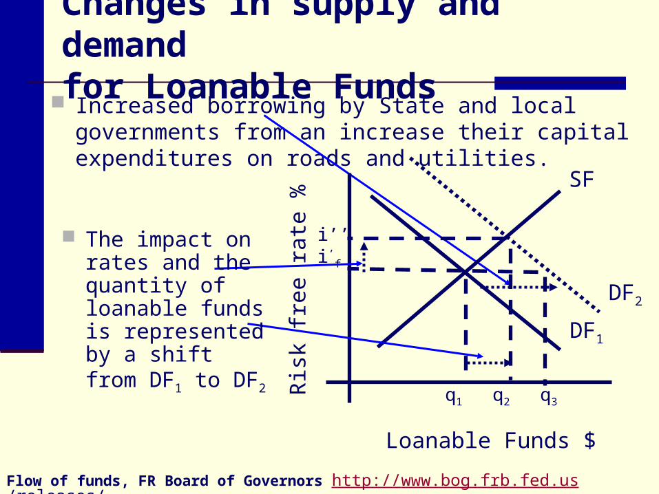
Changes in supply and demand for Loanable Funds

Increased borrowing by State and local governments from an increase their capital expenditures on roads and utilities.

Flow of funds, FR Board of Governors http://www.bog.frb.fed.us/releases/

SF

DF1

Loanable Funds $

Ris

k fr

ee r

ate

%DF2

q1 q2 q3

i’’i’f

The impact on rates and the quantity of loanable funds is represented by a shift from DF1 to DF2

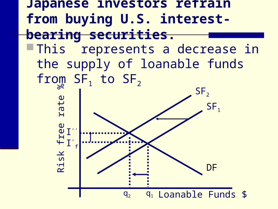
Japanese investors refrain from buying U.S. interest-bearing securities.

This represents a decrease in the supply of loanable funds from SF1 to SF2

Loanable Funds $

Ris

k fr

ee r

ate

%

SF1

DF

SF2

I’’

I’f

q2 q1

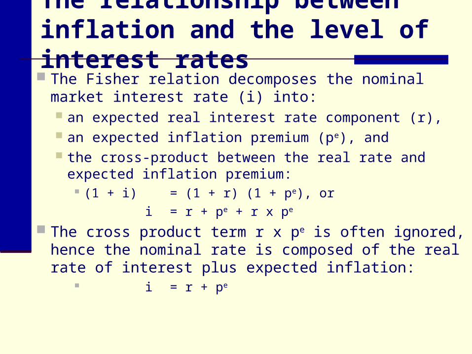
The relationship between inflation and the level of interest rates The Fisher relation decomposes the nominal market

interest rate (i) into: an expected real interest rate component (r), an expected inflation premium (pe), and the cross-product between the real rate and expected

inflation premium: (1 + i) = (1 + r) (1 + pe), or

i = r + pe + r x pe

The cross product term r x pe is often ignored, hence the nominal rate is composed of the real rate of interest plus expected inflation:

i = r + pe

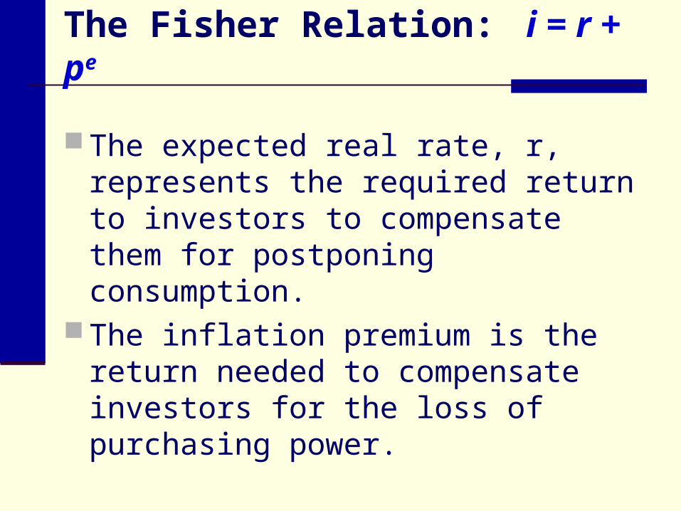
The Fisher Relation: i = r + pe

The expected real rate, r, represents the required return to investors to compensate them for postponing consumption.

The inflation premium is the return needed to compensate investors for the loss of purchasing power.

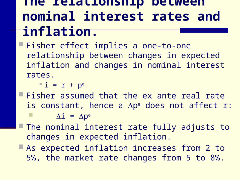
The relationship between nominal interest rates and inflation.

Fisher effect implies a one-to-one relationship between changes in expected inflation and changes in nominal interest rates.

i = r + pe

Fisher assumed that the ex ante real rate is constant, hence a pe does not affect r: i = pe

The nominal interest rate fully adjusts to changes in expected inflation.

As expected inflation increases from 2 to 5%, the market rate changes from 5 to 8%.

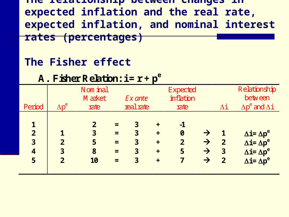
A. Fisher Relation: i = r + pe

Period pe

NominalMarket

rate Ex ante real rate

Expected inflation

rate i

Relationship between

pe and i 1 2 = 3 + -1 2 1 3 = 3 + 0 1 i = pe 3 2 5 = 3 + 2 2 i = pe 4 3 8 = 3 + 5 3 i = pe 5 2 10 = 3 + 7 2 i = pe

The relationship between changes in expected inflation and the real rate, expected inflation, and nominal interest rates (percentages)

The Fisher effect

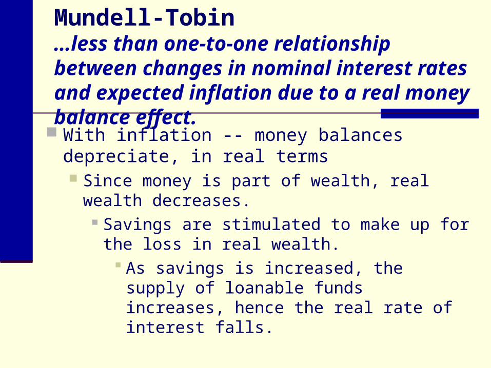
Mundell-Tobin…less than one-to-one relationship between changes in nominal interest rates and expected inflation due to a real money balance effect.

With inflation -- money balances depreciate, in real terms Since money is part of wealth, real wealth

decreases. Savings are stimulated to make up for the

loss in real wealth. As savings is increased, the supply of

loanable funds increases, hence the real rate of interest falls.

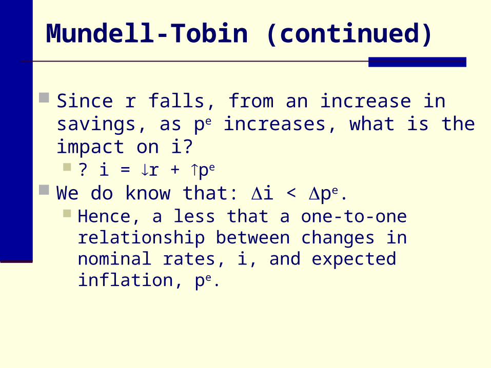
Mundell-Tobin (continued)

Since r falls, from an increase in savings, as pe increases, what is the impact on i? ? i = r + pe

We do know that: i < pe. Hence, a less that a one-to-one relationship

between changes in nominal rates, i, and expected inflation, pe.

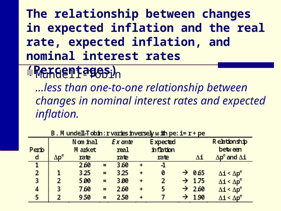
The relationship between changes in expected inflation and the real rate, expected inflation, and nominal interest rates (Percentages)

Mundell-Tobin…less than one-to-one relationship between changes in nominal interest rates and expected inflation.

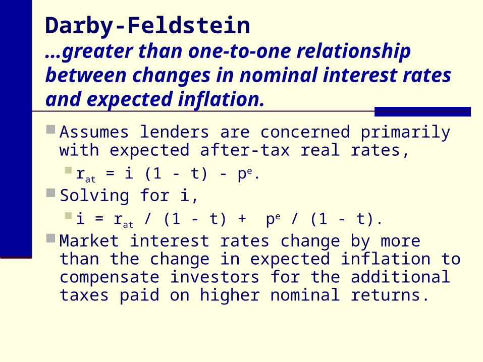
Darby-Feldstein…greater than one-to-one relationship between changes in nominal interest rates and expected inflation.

Assumes lenders are concerned primarily with expected after-tax real rates, rat = i (1 - t) - pe.

Solving for i, i = rat / (1 - t) + pe / (1 - t).

Market interest rates change by more than the change in expected inflation to compensate investors for the additional taxes paid on higher nominal returns.

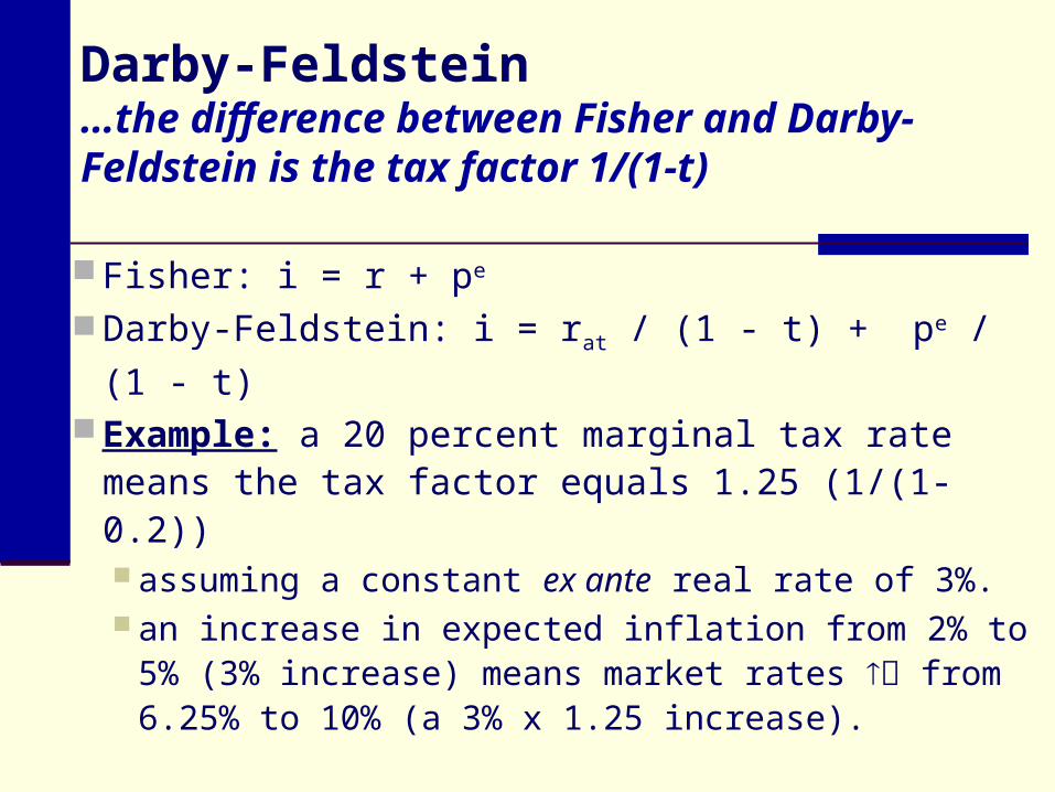
Darby-Feldstein…the difference between Fisher and Darby-Feldstein is the tax factor 1/(1-t)

Fisher: i = r + pe

Darby-Feldstein: i = rat / (1 - t) + pe / (1 - t)

Example: a 20 percent marginal tax rate means the tax factor equals 1.25 (1/(1-0.2)) assuming a constant ex ante real rate of 3%. an increase in expected inflation from 2% to

5% (3% increase) means market rates from 6.25% to 10% (a 3% x 1.25 increase).

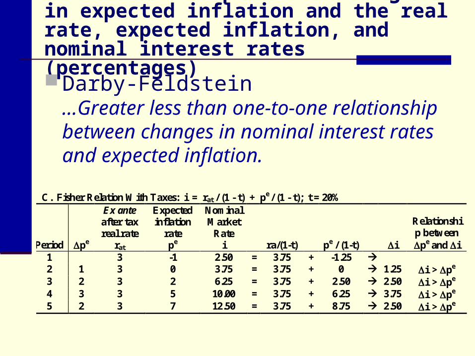
C. Fisher Relation With Taxes: i = rat / (1 - t) + pe / (1 - t); t = 20%

Period pe

Ex ante after tax real rate

rat

Expected inflation

rate pe

Nominal Market

Rate i ra/(1-t) pe / (1-t) i

Relationship between pe and i

1 3 -1 2.50 = 3.75 + -1.25 2 1 3 0 3.75 = 3.75 + 0 1.25 i > pe 3 2 3 2 6.25 = 3.75 + 2.50 2.50 i > pe 4 3 3 5 10.00 = 3.75 + 6.25 3.75 i > pe 5 2 3 7 12.50 = 3.75 + 8.75 2.50 i > pe

The relationship between changes in expected inflation and the real rate, expected inflation, and nominal interest rates (percentages)

Darby-Feldstein…Greater less than one-to-one relationship between changes in nominal interest rates and expected inflation.

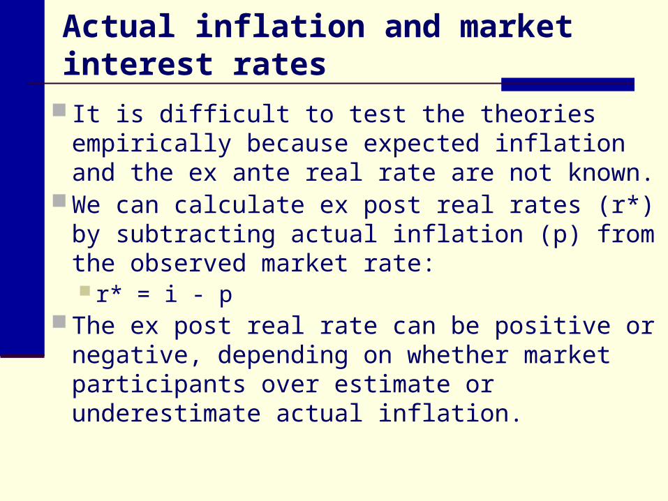
Actual inflation and market interest rates

It is difficult to test the theories empirically because expected inflation and the ex ante real rate are not known.

We can calculate ex post real rates (r*) by subtracting actual inflation (p) from the observed market rate: r* = i - p

The ex post real rate can be positive or negative, depending on whether market participants over estimate or underestimate actual inflation.

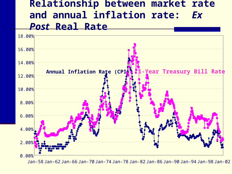
Relationship between market rate and annual inflation rate: Ex Post Real Rate

0.00%

2.00%

4.00%

6.00%

8.00%

10.00%

12.00%

14.00%

16.00%

18.00%

Jan-58 Jan-62 Jan-66 Jan-70 Jan-74 Jan-78 Jan-82 Jan-86 Jan-90 Jan-94 Jan-98 Jan-02

Annual Inflation Rate (CPI) 1-Year Treasury Bill Rate

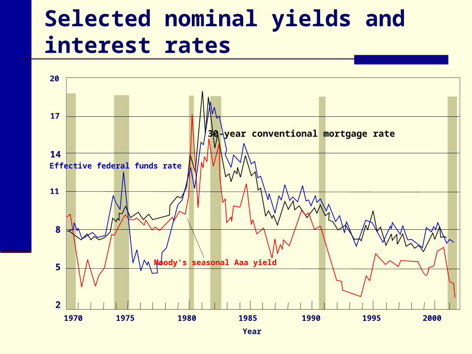
Selected nominal yields and interest rates

20

17

14

11

8

5

21970 1975 1980 1985 1990 1995 2000

Year

Effective federal funds rate

Moody's seasonal Aaa yield

30-year conventional mortgage rate

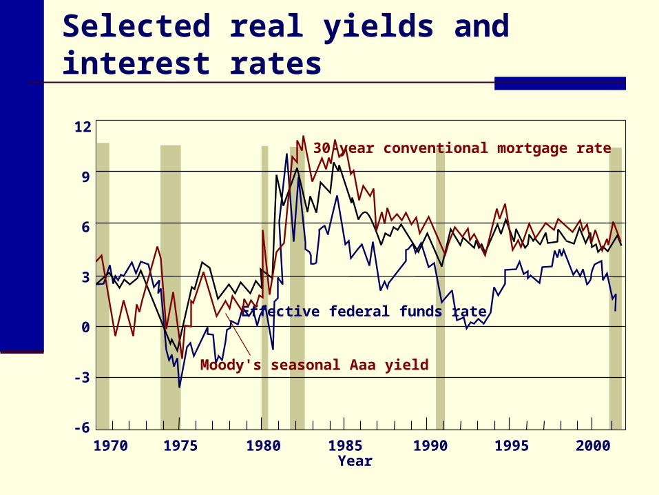
Selected real yields and interest rates

12

9

6

3

0

- 3

- 61970 1975 1980 1985 1990 1995 2000

Year

Effective federal funds rate

30-year conventional mortgage rate

Moody's seasonal Aaa yield

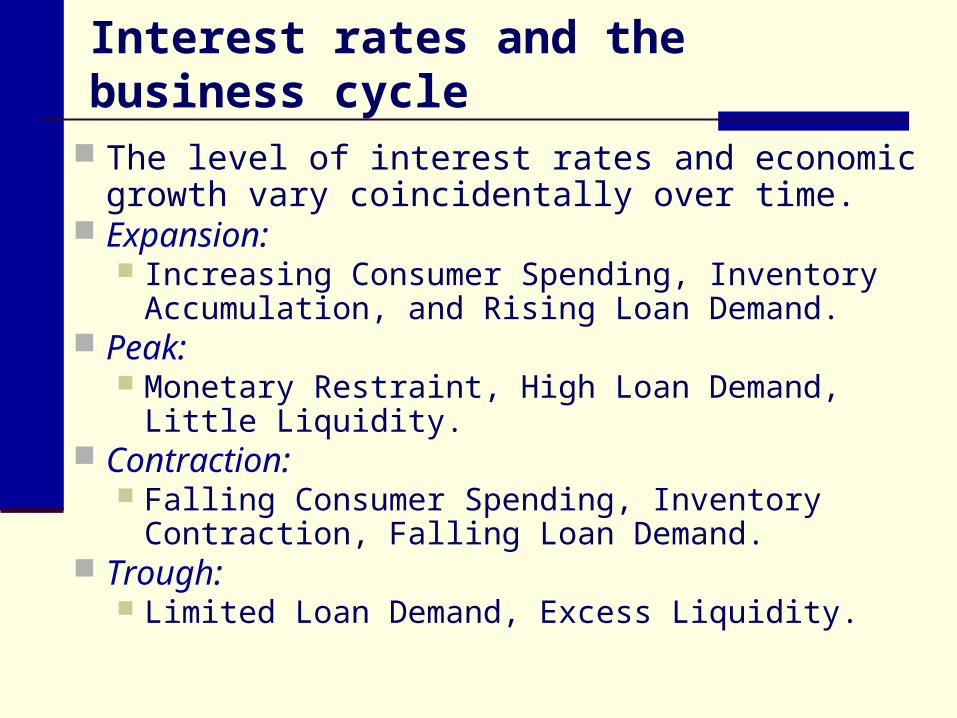
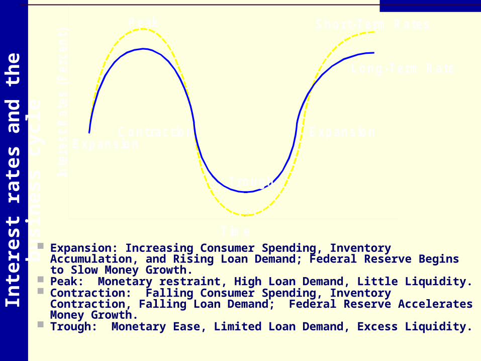
Interest rates and the business cycle

The level of interest rates and economic growth vary coincidentally over time.

Expansion: Increasing Consumer Spending, Inventory

Accumulation, and Rising Loan Demand. Peak:

Monetary Restraint, High Loan Demand, Little Liquidity.

Contraction: Falling Consumer Spending, Inventory Contraction,

Falling Loan Demand. Trough:

Limited Loan Demand, Excess Liquidity.

Tim e

Inte

rest

Rat

es (

Per

cen

t)

E xpansionC ontract ion E xpansion

Long-Term R ates

S hor t -Term R atesP eak

Trough

Inte

rest

rate

s a

nd

th

e b

usin

ess

cycle

Expansion: Increasing Consumer Spending, Inventory Accumulation, and Rising Loan Demand; Federal Reserve Begins to Slow Money Growth.

Peak: Monetary restraint, High Loan Demand, Little Liquidity. Contraction: Falling Consumer Spending, Inventory Contraction,

Falling Loan Demand; Federal Reserve Accelerates Money Growth. Trough: Monetary Ease, Limited Loan Demand, Excess Liquidity.

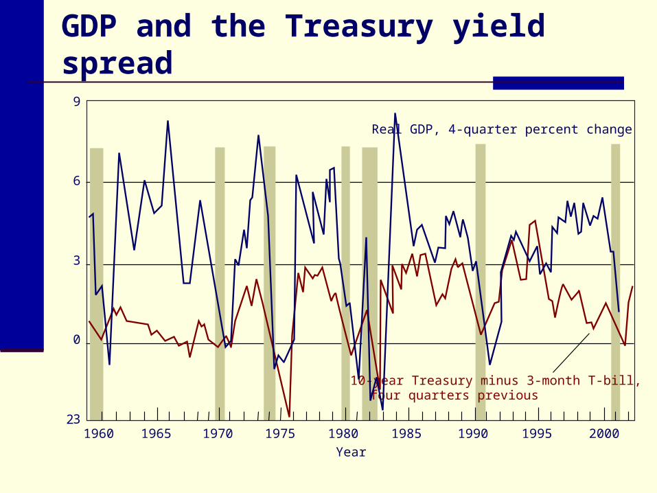
GDP and the Treasury yield spread

9

6

3

0

231960 1965 1970 1975 1980 1985 1990 1995 2000

Year

Real GDP, 4-quarter percent change

10-year Treasury minus 3-month T-bill, four quarters previous

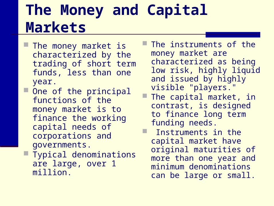
The Money and Capital Markets

The money market is characterized by the trading of short term funds, less than one year.

One of the principal functions of the money market is to finance the working capital needs of corporations and governments.

Typical denominations are large, over 1 million.

The instruments of the money market are characterized as being low risk, highly liquid and issued by highly visible "players."

The capital market, in contrast, is designed to finance long term funding needs.

Instruments in the capital market have original maturities of more than one year and minimum denominations can be large or small.

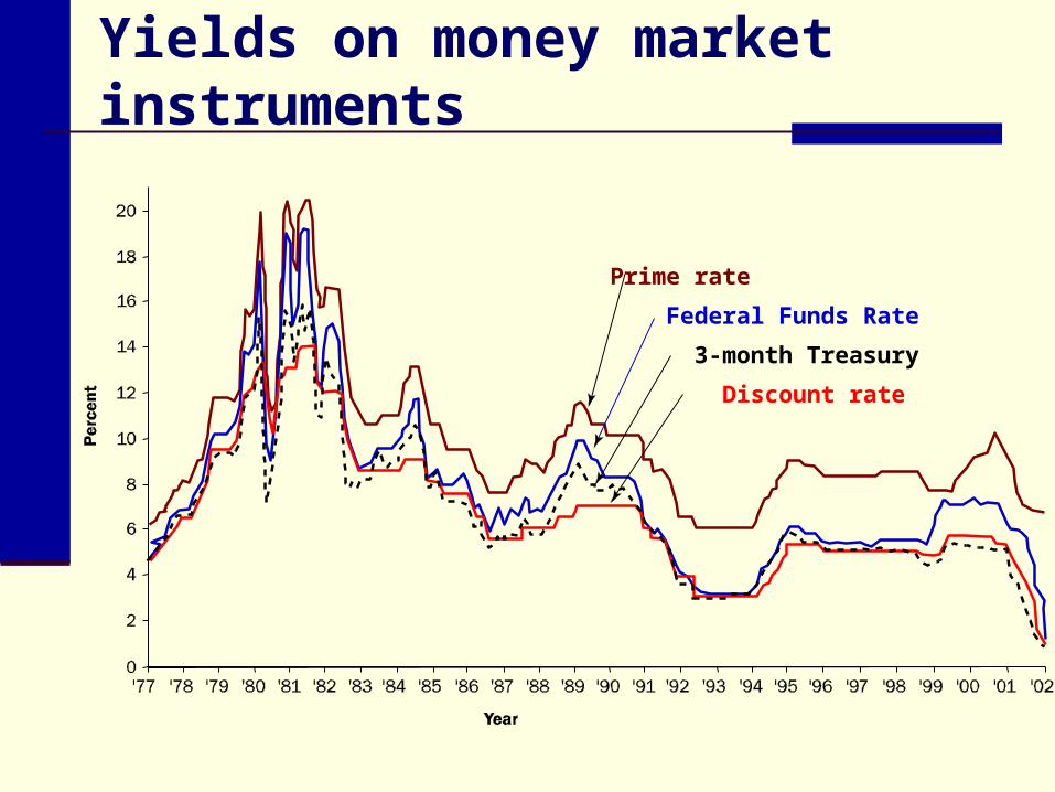
Yields on money market instruments

Prime rate

Federal Funds Rate

3-month Treasury

Discount rate

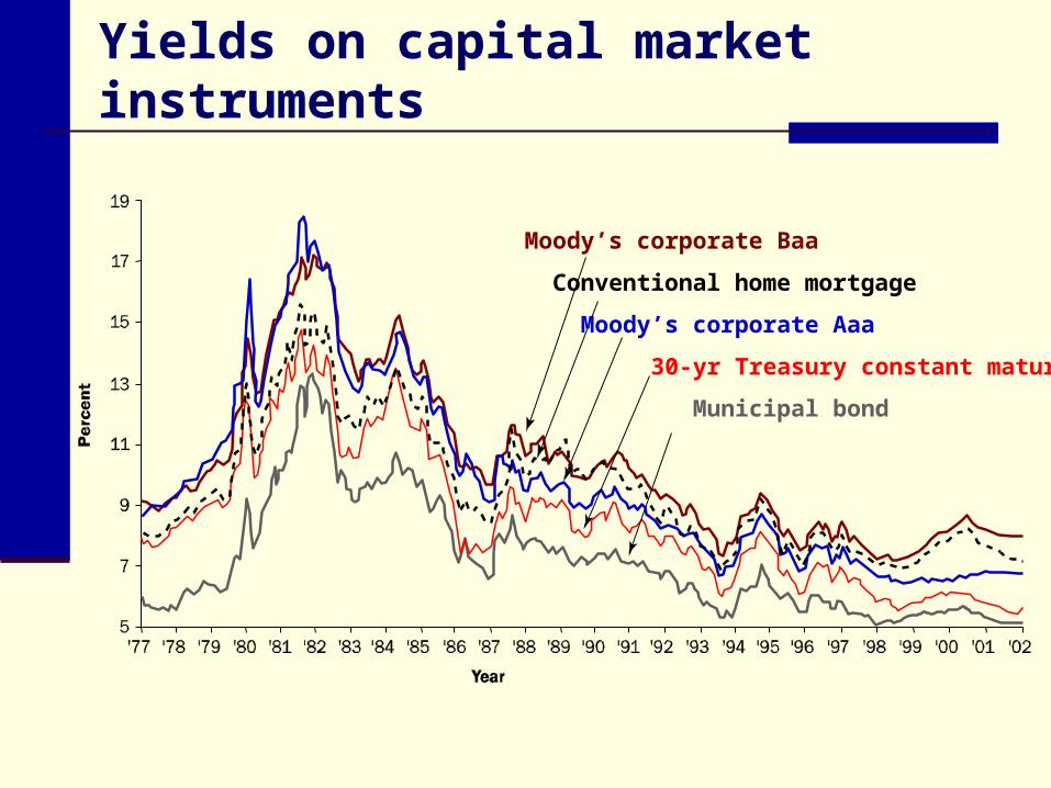
Yields on capital market instruments

Moody’s corporate Baa

Conventional home mortgage

Moody’s corporate Aaa

30-yr Treasury constant maturity

Municipal bond

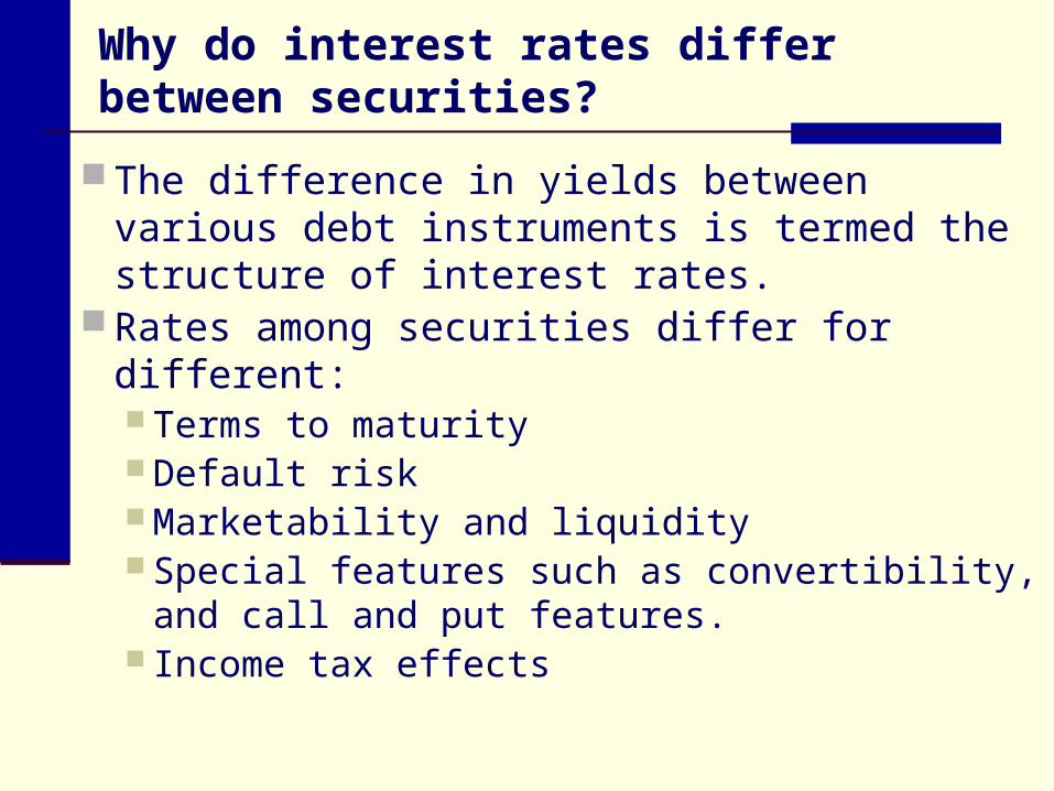
Why do interest rates differ between securities?

The difference in yields between various debt instruments is termed the structure of interest rates.

Rates among securities differ for different: Terms to maturity Default risk Marketability and liquidity Special features such as convertibility, and

call and put features. Income tax effects

Term to final maturity

In general, the longer the maturity, the greater are these risks.

Yield Curve…a diagram that compares the market yields on securities that differ only in terms of maturity. The general relationship is also referred to

as the term structure of interest rates.

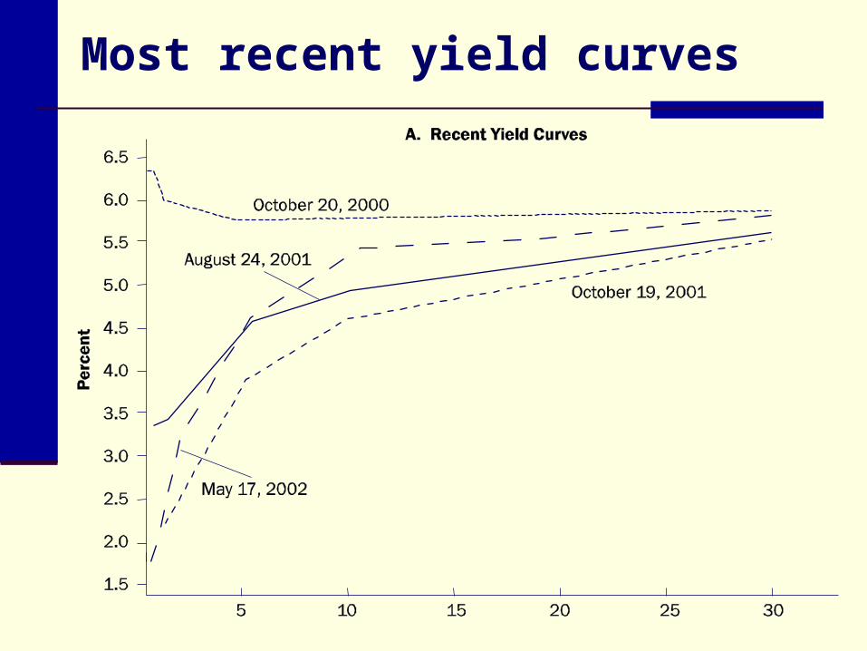
Most recent yield curves

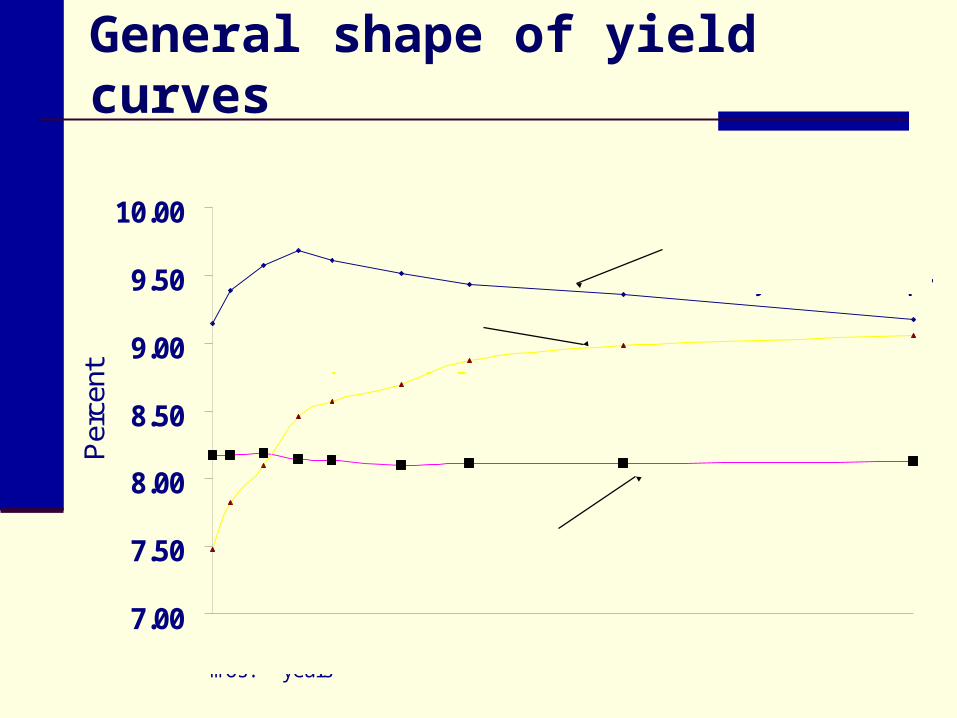
General shape of yield curves

7.00

7.50

8.00

8.50

9.00

9.50

10.00

Per

cent

March 1989Generally Downward Sloping

September 1988Upward Sloping

August 1989Flat Yield Curve

| | | | | | | | | 3 6 1 2 3 5 7 10 30 mos. years

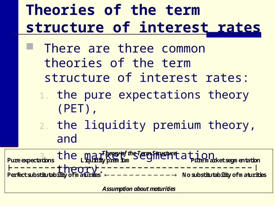
Theory of the Term Structure

Pure expectations Liquidity premium Pure market segmentation |——————————————|——————————————————————————| Perfect substitutability of maturites No substitutability of maturities

Assumption about maturities

Theories of the term structure of interest rates There are three common theories of the

term structure of interest rates:1. the pure expectations theory (PET),

2. the liquidity premium theory, and

3. the market segmentation theory.

Unbiased expectations theory…Attributes the relationship between yields on different maturity securities entirely to difference in expectations of future interest rates.

Long-term interest rates are an average of current and expected short-term interest rates.

The expected short-term interest rate is the market's unbiased forecast of future interest rates.

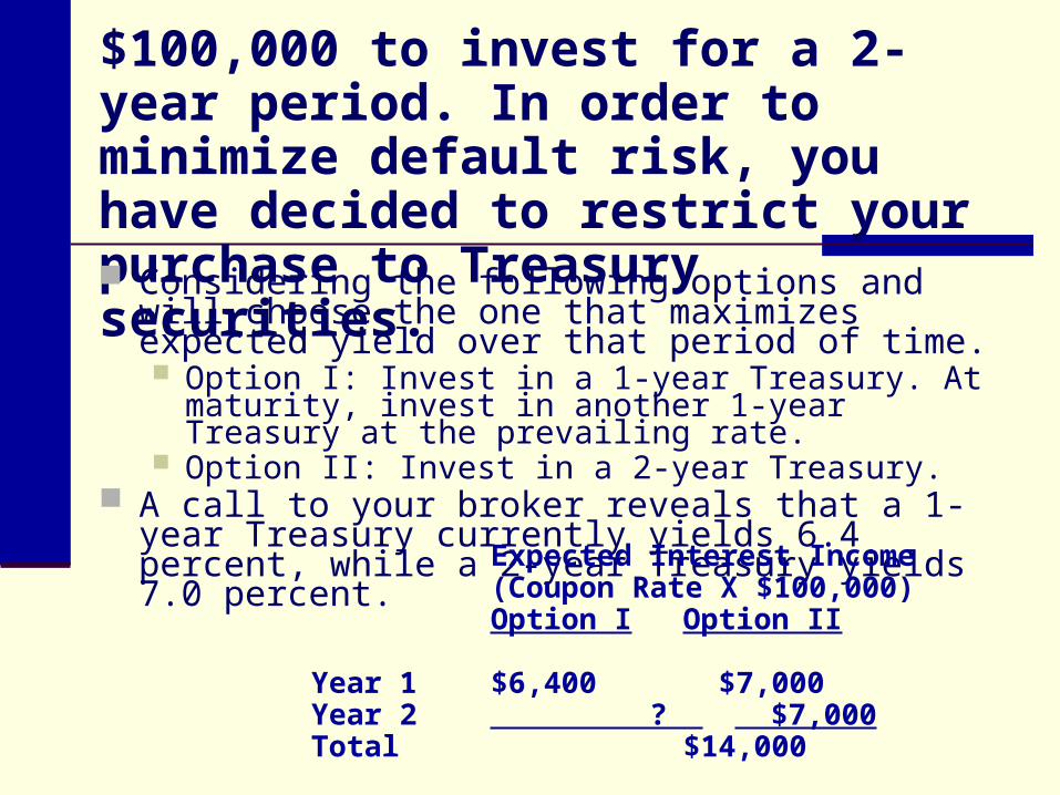
$100,000 to invest for a 2-year period. In order to minimize default risk, you have decided to restrict your purchase to Treasury securities. Considering the following options and will choose the

one that maximizes expected yield over that period of time. Option I: Invest in a 1-year Treasury. At maturity, invest in

another 1-year Treasury at the prevailing rate. Option II: Invest in a 2-year Treasury.

A call to your broker reveals that a 1-year Treasury currently yields 6.4 percent, while a 2-year Treasury yields 7.0 percent.

Expected Interest Income(Coupon Rate X $100,000)Option I Option II

Year 1 $6,400 $7,000Year 2 ? $7,000Total $14,000

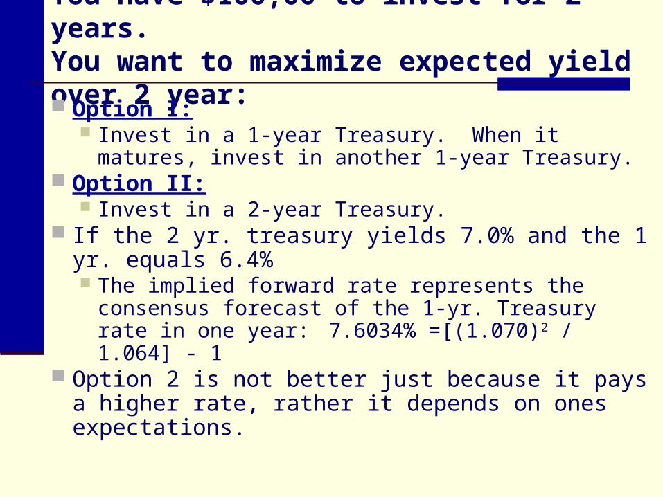
You have $100,00 to invest for 2 years.You want to maximize expected yield over 2 year:

Option I: Invest in a 1-year Treasury. When it matures,

invest in another 1-year Treasury. Option II:

Invest in a 2-year Treasury. If the 2 yr. treasury yields 7.0% and the 1 yr.

equals 6.4% The implied forward rate represents the consensus

forecast of the 1-yr. Treasury rate in one year:7.6034% =[(1.070)2 / 1.064] - 1

Option 2 is not better just because it pays a higher rate, rather it depends on ones expectations.

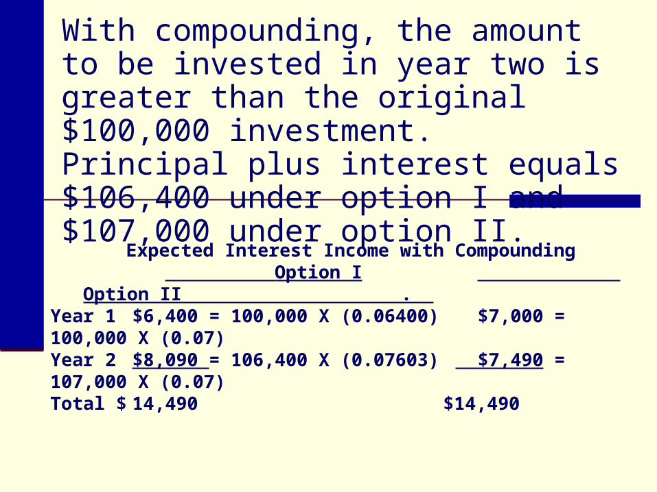
With compounding, the amount to be invested in year two is greater than the original $100,000 investment. Principal plus interest equals $106,400 under option I and $107,000 under option II.

Expected Interest Income with Compounding Option I Option II

. Year 1 $6,400 = 100,000 X (0.06400) $7,000 = 100,000 X (0.07) Year 2 $8,090 = 106,400 X (0.07603) $7,490 = 107,000 X (0.07) Total $ 14,490 $14,490

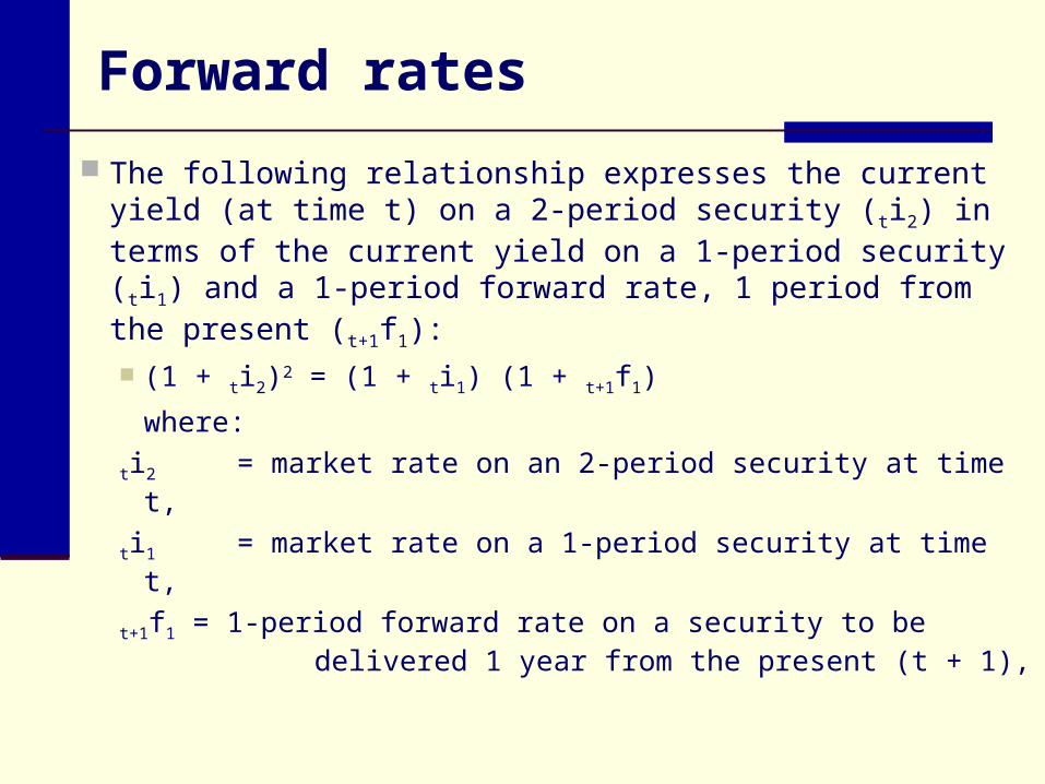
Forward rates

The following relationship expresses the current yield (at time t) on a 2-period security (ti2) in terms of the current yield on a 1-period security (ti1) and a 1-period forward rate, 1 period from the present (t+1f1): (1 + ti2)2 = (1 + ti1) (1 + t+1f1)

where:

ti2 = market rate on an 2-period security at time t,

ti1 = market rate on a 1-period security at time t,

t+1f1 = 1-period forward rate on a security to be delivered 1 year from the present (t + 1),

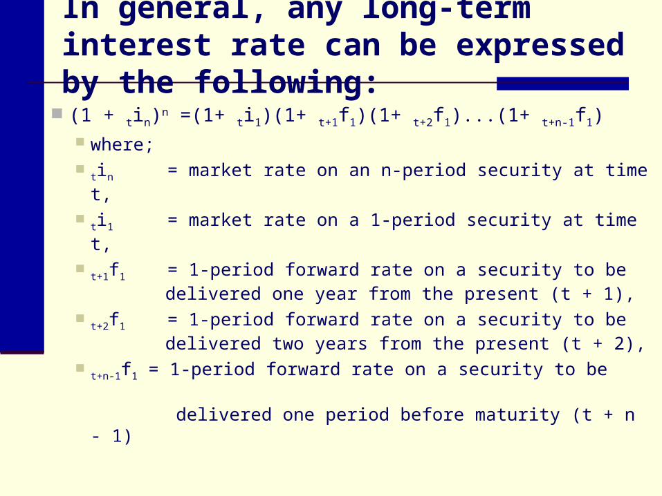
In general, any long-term interest rate can be expressed by the following:

(1 + tin)n =(1+ ti1)(1+ t+1f1)(1+ t+2f1)...(1+ t+n-1f1) where;

tin = market rate on an n-period security at time t,

ti1 = market rate on a 1-period security at time t,

t+1f1 = 1-period forward rate on a security to be delivered one year from the present (t + 1),

t+2f1 = 1-period forward rate on a security to be delivered two years from the present (t + 2),

t+n-1f1 = 1-period forward rate on a security to be delivered one period before maturity (t + n - 1)

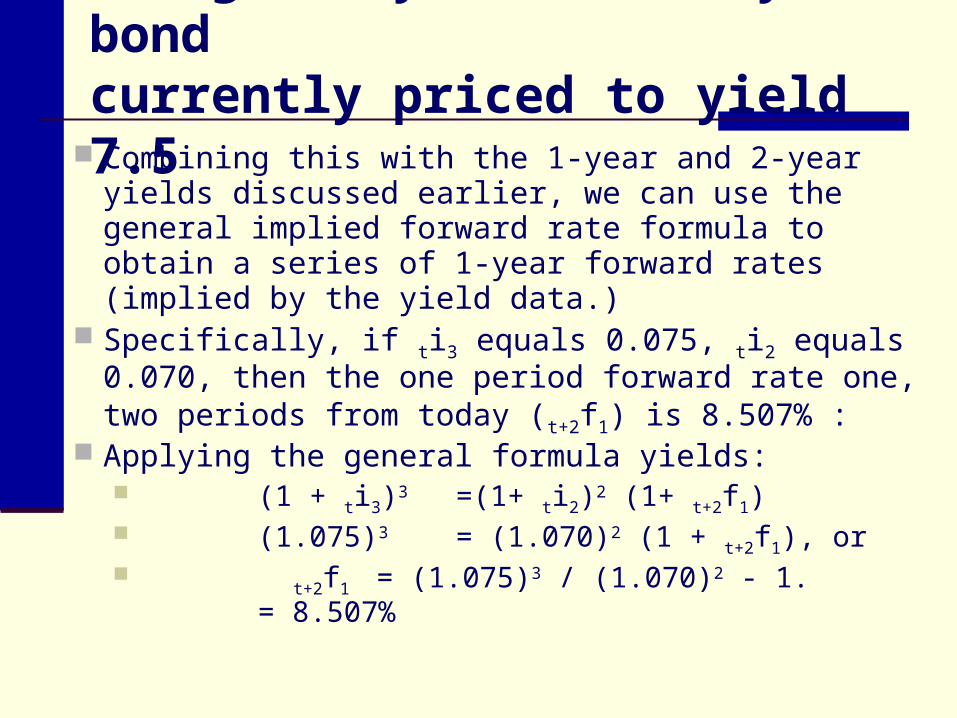
Using a 3-year Treasury bondcurrently priced to yield 7.5

Combining this with the 1-year and 2-year yields discussed earlier, we can use the general implied forward rate formula to obtain a series of 1-year forward rates (implied by the yield data.)

Specifically, if ti3 equals 0.075, ti2 equals 0.070, then the one period forward rate one, two periods from today (t+2f1) is 8.507% :

Applying the general formula yields: (1 + ti3)3 =(1+ ti2)2 (1+ t+2f1) (1.075)3 = (1.070)2 (1 + t+2f1), or t+2f1 = (1.075)3 / (1.070)2 - 1.

= 8.507%

Liquidity premium theory…extends the unbiased expectations theory by incorporating investor expectations of price risk in establishing market rates.

The unbiased expectations theory assumes that securities that differ only in terms of maturity are perfect substitutes.

If the expected return on a series of short-term securities equals the expected return on a long-term security, investors will prefer the short-term securities.

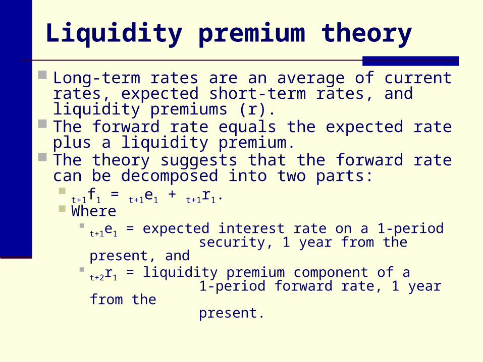
Liquidity premium theory

Long-term rates are an average of current rates, expected short-term rates, and liquidity premiums (r).

The forward rate equals the expected rate plus a liquidity premium.

The theory suggests that the forward rate can be decomposed into two parts:

t+1f1 = t+1e1 + t+1r1. Where

t+1e1 = expected interest rate on a 1-period security, 1 year from the present, and

t+2r1 = liquidity premium component of a

1-period forward rate, 1 year from the present.

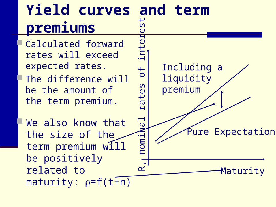
Yield curves and term premiums

Calculated forward rates will exceed expected rates.

The difference will be the amount of the term premium.

Pure Expectations

Including a liquidity premium

R,

nom

inal

rat

es o

f in

tere

st

Maturity

We also know that the size of the term premium will be positively related to maturity: =f(t+n)

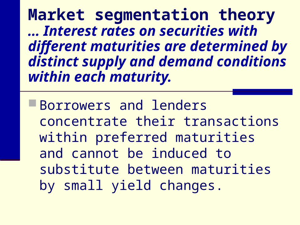
Market segmentation theory… Interest rates on securities with different maturities are determined by distinct supply and demand conditions within each maturity.

Borrowers and lenders concentrate their transactions within preferred maturities and cannot be induced to substitute between maturities by small yield changes.

Market segmentation theory (continued)

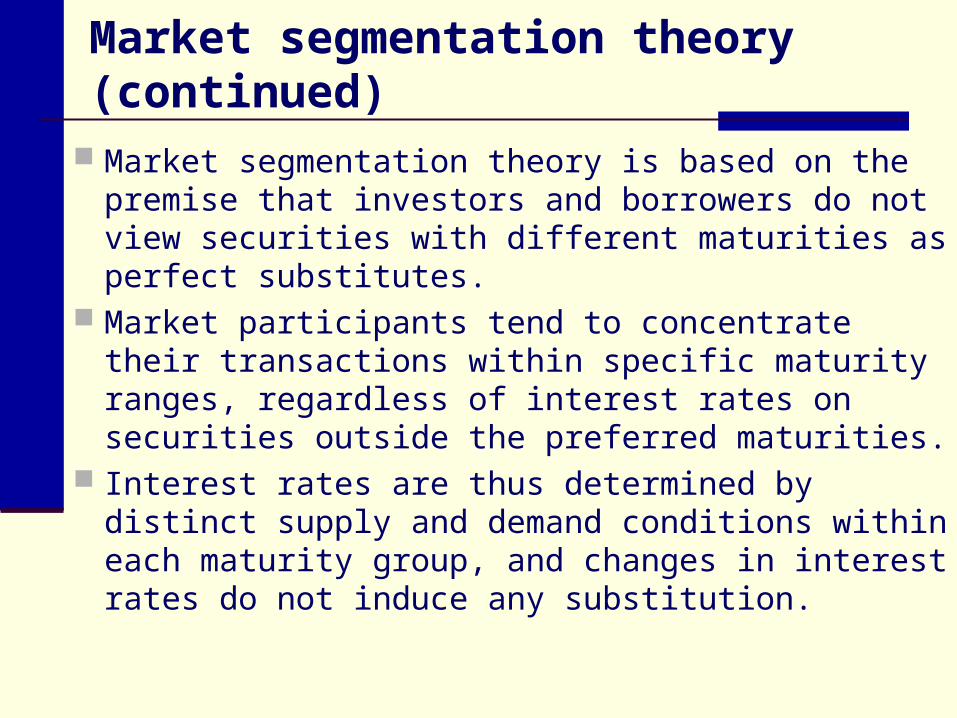
Market segmentation theory is based on the premise that investors and borrowers do not view securities with different maturities as perfect substitutes.

Market participants tend to concentrate their transactions within specific maturity ranges, regardless of interest rates on securities outside the preferred maturities.

Interest rates are thus determined by distinct supply and demand conditions within each maturity group, and changes in interest rates do not induce any substitution.

Market segmentation theory (continued)

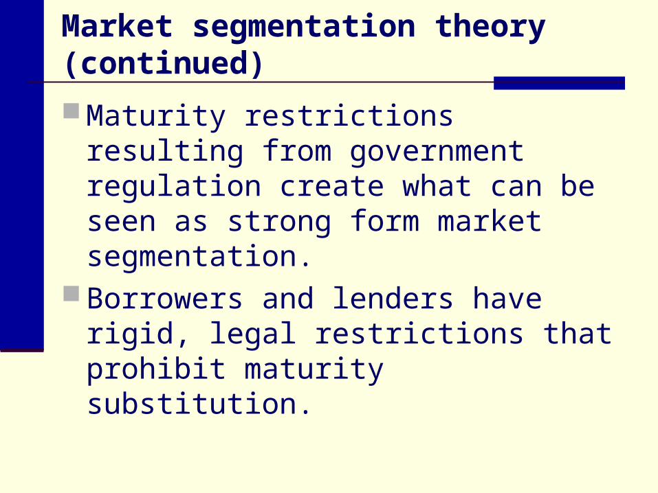
Maturity restrictions resulting from government regulation create what can be seen as strong form market segmentation.

Borrowers and lenders have rigid, legal restrictions that prohibit maturity substitution.

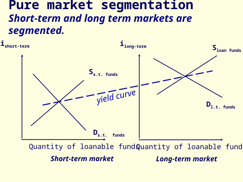
Pure market segmentationShort-term and long term markets are segmented.

Short-term market

Ds.t. funds

Ss.t. funds

ishort-term

Quantity of loanable funds

yield curve

Long-term market

Dl.t. funds

Sloan funds

Quantity of loanable funds

ilong-term

The yield curve and the business cycle

During the early stages of expansion, unemployment and inflation are relative low, typically we see and upward sloping yield curve.

At the peak, loan demand is high, inflation is high and rising and the Fed acts to reduce the growth in loanable funds, thus we often see a flat or downward sloping yield curve.

Term to repricing for variable rate and floating rate securities

A security is classified as variable rate if the applicable market interest rate is reset at predetermined intervals.

The security is classified as floating rate if the applicable market interest rate is tied to some index and changes whenever the index changes.

LIBOR, a popular floating rate index, is the London Interbank Offer Rate.

Default risk…the probability or likelihood that a borrower will not make the contractual interest and principal payments.

A default risk premium is the difference between the yield on a risk security and a comparable Treasury security: drp = ir - it , where

ir = interest rate on a security subject to default risk, it = interest rate on a Treasury, and drp= default risk premium,

The risk premium will always be positive since risky securities offer higher yields than comparable Treasury securities.

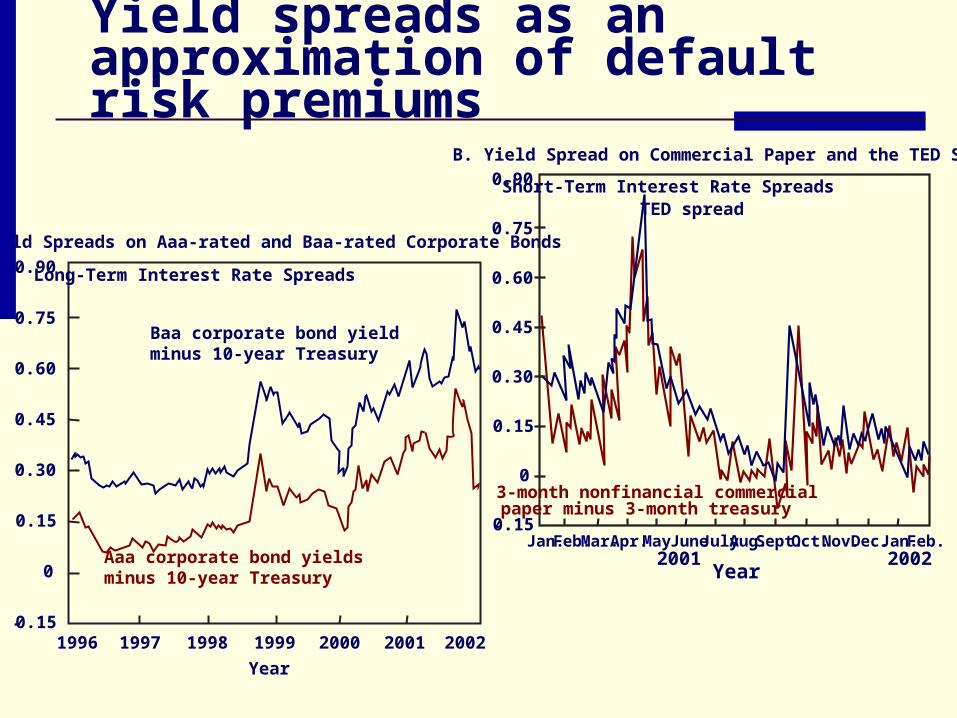
Yield spreads as an approximation of default risk premiums

0.90

0.75

0.60

0.45

0.30

0.15

0

- 0.151996 1997 1998 1999 2000 2001 2002

Aaa corporate bond yields minus 10-year Treasury

Baa corporate bond yield minus 10-year Treasury

Long-Term Interest Rate Spreads

Year

A. Yield Spreads on Aaa-rated and Baa-rated Corporate Bonds

0.90

0.75

0.60

0.45

0.30

0.15

0

-0.15Jan.Feb.Mar. Apr.May June JulyAug.Sept. Oct. Nov.Dec. Jan.Feb.

2001 2002

3-month nonfinancial commercialpaper minus 3-month treasury

TED spreadShort-Term Interest Rate Spreads

Year

B. Yield Spread on Commercial Paper and the TED Spread

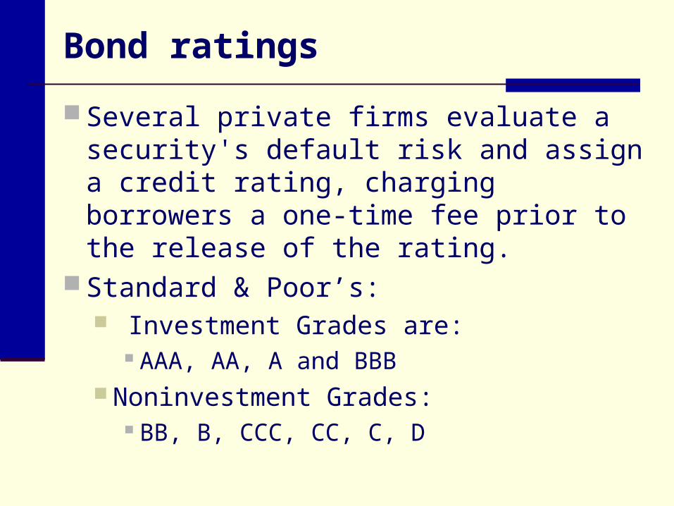
Bond ratings

Several private firms evaluate a security's default risk and assign a credit rating, charging borrowers a one-time fee prior to the release of the rating.

Standard & Poor’s: Investment Grades are:

AAA, AA, A and BBB Noninvestment Grades:

BB, B, CCC, CC, C, D

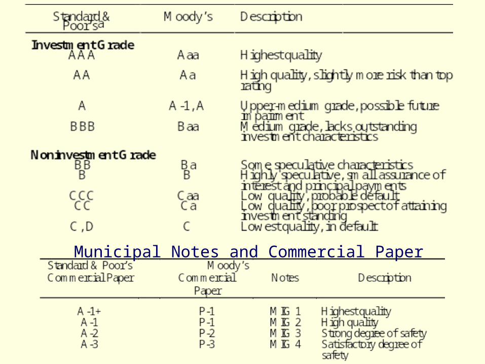
Municipal Notes and Commercial Paper

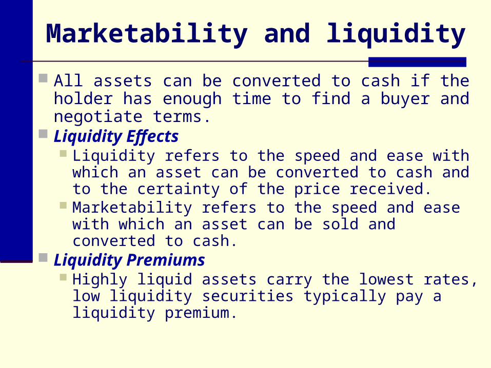
Marketability and liquidity

All assets can be converted to cash if the holder has enough time to find a buyer and negotiate terms.

Liquidity Effects Liquidity refers to the speed and ease with which an

asset can be converted to cash and to the certainty of the price received.

Marketability refers to the speed and ease with which an asset can be sold and converted to cash.

Liquidity Premiums Highly liquid assets carry the lowest rates, low

liquidity securities typically pay a liquidity premium.

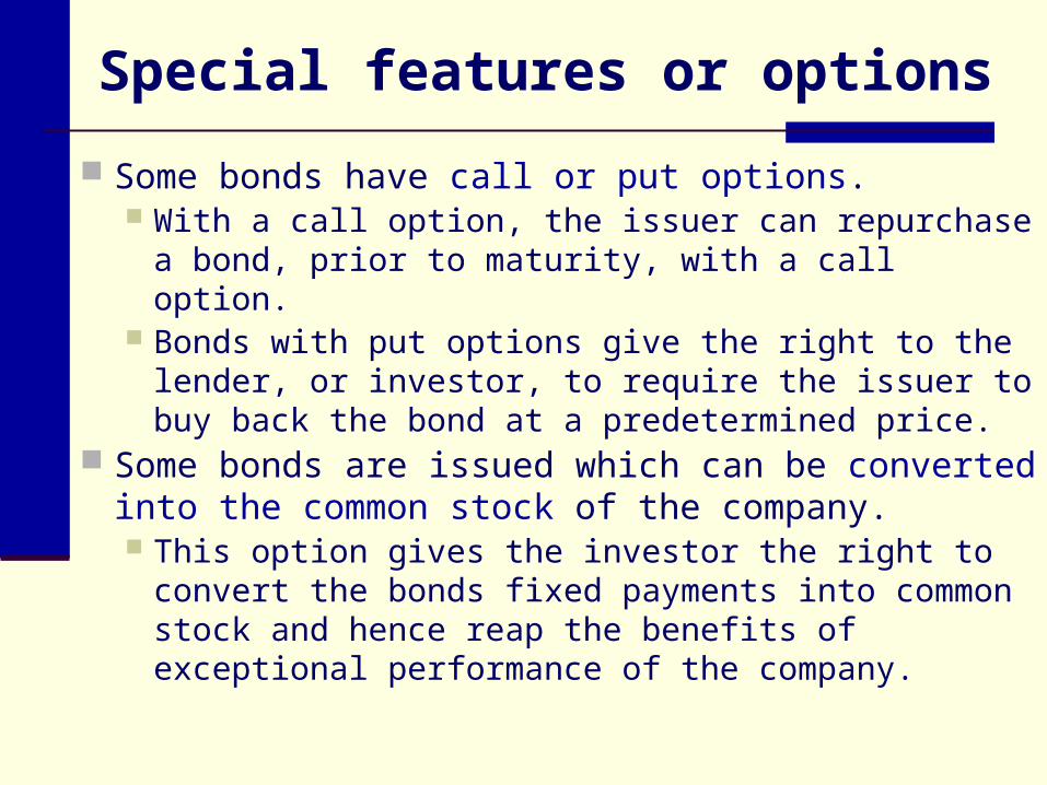
Special features or options

Some bonds have call or put options. With a call option, the issuer can repurchase a bond,

prior to maturity, with a call option. Bonds with put options give the right to the lender, or

investor, to require the issuer to buy back the bond at a predetermined price.

Some bonds are issued which can be converted into the common stock of the company. This option gives the investor the right to convert the

bonds fixed payments into common stock and hence reap the benefits of exceptional performance of the company.

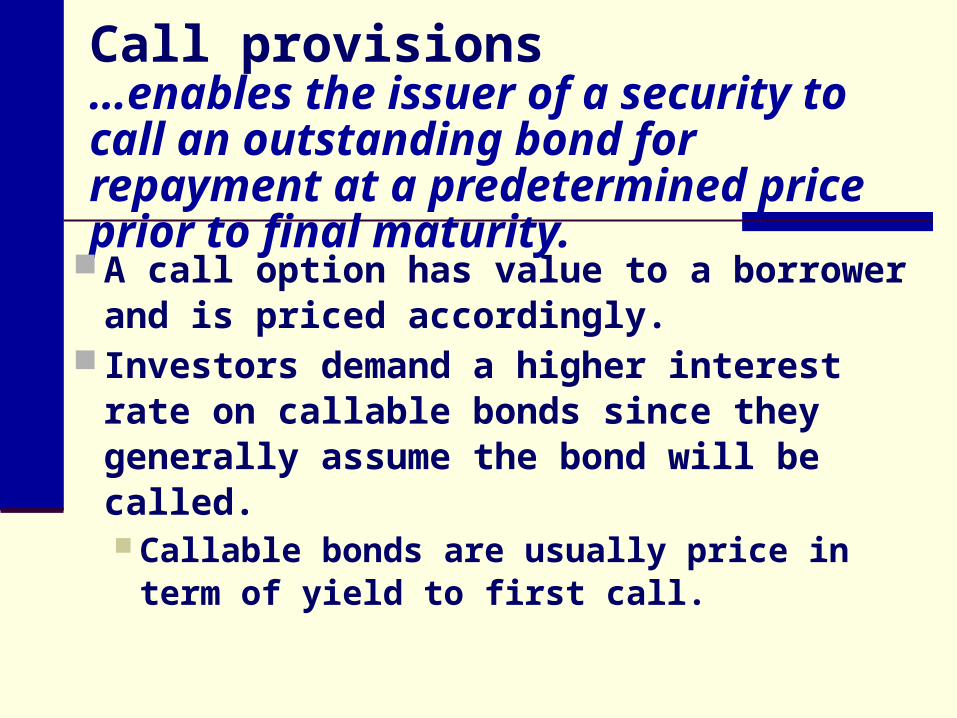
Call provisions…enables the issuer of a security to call an outstanding bond for repayment at a predetermined price prior to final maturity.

A call option has value to a borrower and is priced accordingly.

Investors demand a higher interest rate on callable bonds since they generally assume the bond will be called. Callable bonds are usually price in term

of yield to first call.

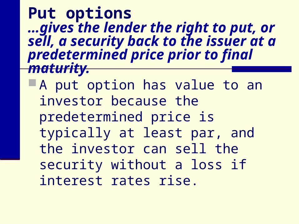
Put options…gives the lender the right to put, or sell, a security back to the issuer at a predetermined price prior to final maturity.

A put option has value to an investor because the predetermined price is typically at least par, and the investor can sell the security without a loss if interest rates rise.

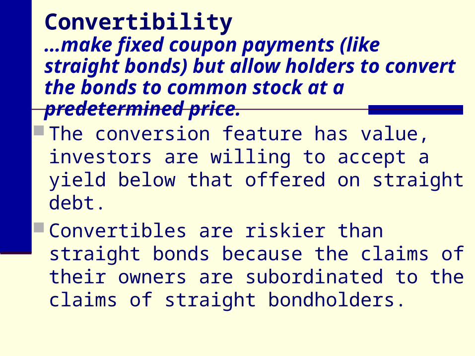
Convertibility…make fixed coupon payments (like straight bonds) but allow holders to convert the bonds to common stock at a predetermined price.

The conversion feature has value, investors are willing to accept a yield below that offered on straight debt.

Convertibles are riskier than straight bonds because the claims of their owners are subordinated to the claims of straight bondholders.

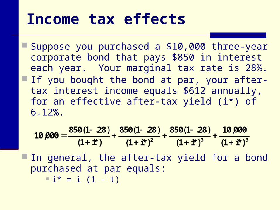
Income tax effects

Suppose you purchased a $10,000 three-year corporate bond that pays $850 in interest each year. Your marginal tax rate is 28%.

If you bought the bond at par, your after-tax interest income equals $612 annually, for an effective after-tax yield (i*) of 6.12%.

In general, the after-tax yield for a bond purchased at par equals:

i* = i (1 - t)

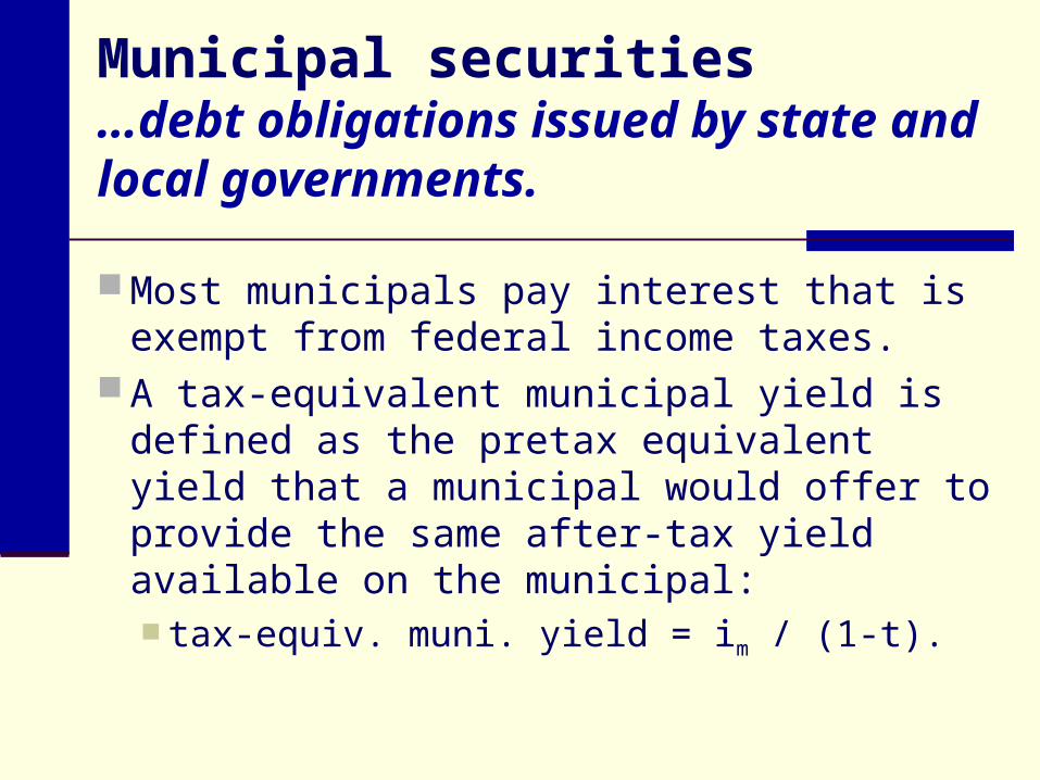
Municipal securities…debt obligations issued by state and local governments.

Most municipals pay interest that is exempt from federal income taxes.

A tax-equivalent municipal yield is defined as the pretax equivalent yield that a municipal would offer to provide the same after-tax yield available on the municipal: tax-equiv. muni. yield = im / (1-t).

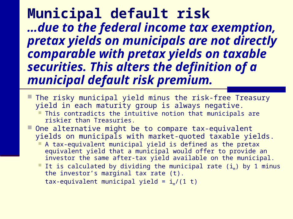
Municipal default risk …due to the federal income tax exemption, pretax yields on municipals are not directly comparable with pretax yields on taxable securities. This alters the definition of a municipal default risk premium. The risky municipal yield minus the risk-free Treasury yield in each

maturity group is always negative. This contradicts the intuitive notion that municipals are riskier than

Treasuries. One alternative might be to compare tax-equivalent yields on

municipals with market-quoted taxable yields. A tax-equivalent municipal yield is defined as the pretax equivalent yield

that a municipal would offer to provide an investor the same after-tax yield available on the municipal.

It is calculated by dividing the municipal rate (im) by 1 minus the investor’s marginal tax rate (t).

tax-equivalent municipal yield = im/(1 t)

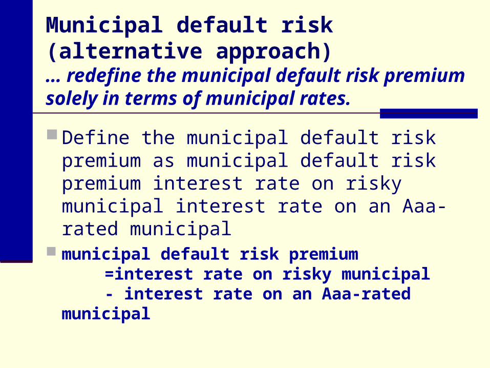
Municipal default risk (alternative approach)… redefine the municipal default risk premium solely in terms of municipal rates.

Define the municipal default risk premium as municipal default risk premium interest rate on risky municipal interest rate on an Aaa-rated municipal

municipal default risk premium =interest rate on risky municipal - interest rate on an Aaa-rated

municipal

THE DETERMINATES OF INTEREST RATES

Chapter 7

Bank ManagementBank Management, 5th edition.5th edition.Timothy W. Koch and S. Scott MacDonaldTimothy W. Koch and S. Scott MacDonaldCopyright © 2003 by South-Western, a division of Thomson Learning