a biological survey of the south east south australia

A BIOLOGICAL SURVEY OF

THE SOUTH EAST

SOUTH AUSTRALIA

1991 and 1997

Editors

J. N. Foulkes Biological Survey and Monitoring

Science and Conservation Directorate

Department for Environment and Heritage, South Australia

L. M. B. Heard Environmental Analysis and Research Unit

Environmental Information Directorate

Department for Environment and Heritage, South Australia

2003

South East Biological Survey

The Biological Survey of the South East, South Australia was carried out with the assistance of funds made

available by the Commonwealth of Australia under the National Estate Grants Programs and the State

Government of South Australia.

The views and opinions expressed in this report are those of the authors and do not necessarily represent the

views or policies of the Australian Heritage Commission or the State Government of South Australia.

This report may be cited as:

Foulkes, J. N. and Heard, L. M. B. (Eds.) (2003). A Biological Survey of the South East, South Australia. 1991and 1997. (Department for Environment and Heritage, South Australia).

Copies of the report may be accessed in the library:

State Library of South Australia

North Terrace, ADELAIDE SA 5000

EDITORS

J. N. Foulkes and L. M. B. Heard

Biological Survey and Monitoring Section, Science and Conservation Directorate,

Department for Environment and Heritage, GPO Box 1047 ADELAIDE SA 5001

AUTHORS

T. Croft, J. N. Foulkes, D. Hopton, H. M. Owens, L. F. Queale, Biological Survey and Monitoring Section,

Science and Conservation Directorate, Department for Environment and Heritage, GPO Box 1047 ADELAIDE

SA 5001.

G. Carpenter, Biodiversity Assessment Services, Department for Water, Land and Biodiversity Conservation,

BO Box 2834 ADELAIDE SA 5001

L. M. B. Heard, F.M. Smith, Environmental Analysis and Research Unit, Department for Environment and

Heritage, PO Box 550, MARLESTON SA 5033.

M. Benbow, Latlong Enterprises, PO Box 458, KAPUNDA SA 5373.

GEOGRAPHIC INFORMATION SYSTEMS (GIS) ANALYSIS AND PRODUCT DEVELOPMENT

Vegetation Component:

Environmental Analysis and Research Unit, Department for Environment and Heritage

Fauna Component:

Biodiversity Survey and Monitoring, Biodiversity Strategies Branch, Department for Environment and Heritage

COVER DESIGN

Public Communications and Visitor Services, Department for Environment and Heritage.

PRINTED BY

JMJ Printing Services, ADELAIDE

© Department for Environment and Heritage 2003.

ISBN 7590 1050 1

Cover Photograph: Stringybark Woodland, The Bluff Native Forest Reserve, ESE of Tantanoola.

Photo: L. M. B. Heard

ii


PREFACEA Biological Survey of the South East, South Australia is a further product of the Biological Survey of South Australia.

The program of systematic biological surveys to cover the whole of South Australia arose out of a realisation that an

effort was needed to increase our knowledge of the remaining vascular plants and vertebrate fauna of South Australia

and to encourage its conservation.

Over the last 18 years, there has been a strong commitment to the Biological Survey by Government and an impressive

dedication from hundreds of volunteer biologists.

By 2015, it is anticipated that the Biological Survey will achieve complete statewide coverage.

The Biological Survey of South Australia will be an achievement for which we can be very proud. We will have

substantially improved our knowledge of the biodiversity of South Australia to enable biologists in the future to measure

the direction of long-term ecological change. This will greatly enhance our ability to adequately manage nature

conservation into the future.

JOHN HILL

MINISTER FOR ENVIRONMENT AND CONSERVATION

iii

ABSTRACT


A vegetation survey was carried out in the South East in 1991 that sampled 340 quadrats. This was followed by a

vertebrate survey in January-February 1997 that sampled a sub-set of 96 quadrats. These sites aimed to sample

representative areas of all the remaining natural vegetation in the area in proportion to the broad habitat variability of the

total area. In addition, at least one sampling site was located in the majority of the reserves under the National Parks and

Wildlife Act (1972) in the study area. The total number of records contributed to the Biological Survey Database as a

result of this survey were: 23, 212 plants, 1,579 amphibians, 676 reptiles, 3,168 birds and 1276 mammals.

A combined analysis of the plant quadrat data with a sub-set of Murray Mallee and South East Coast plant data resulted

in the description of 29 PATN floristic groups. Using this analysis as a basis, a vegetation map of the South East was

produced comprising 54 regional plant communities based on the dominant upper-storey plant. Using these 54 regional

communities, 362 unique combinations (pure communities and mosaics of communities) have been identified and

mapped.

A combined analysis of the fauna quadrat data and data from eight other fauna surveys was undertaken. PATN analysis

of the combined data set comprising 165 quadrats revealed six communities. PATN analyses on reptiles and birds

tended to show clear patterning, however some groups were poorly defined. The reptile analysis resulted in the

recognition of five communities with definite habitat preferences for species defined. Similarly, five bird communities

were recognised, some of which appeared to have more ecological integrity than others.

Of 62 reptile species known from the area, 41 species were recorded during the South East Survey. Populations of the

Swamp Skink and Glossy Grass Skink are significant for the overall conservation of these species. There were nine

species of amphibians recorded during the survey of the 12 known from the region.

One hundred and sixty eight of the two hundred and fifty-seven species of birds were recorded from the study area during the

survey. Eight exotic species were recorded from quadrats during the survey. Bird species of conservation significance include:

Malleefowl, Rufous Bristlebird, and Red Tailed Black Cockatoo.

The South East Survey recorded 21 extant mammal species of the 60 recorded from the area. Eleven species were exotic.

Native terrestrial mammal captures and observations were low, even of species perceived as common. This raises some

serious concerns for the long-term survival of small mammal communities in the South East.

iv


CONTENTS

Preface ................................................................................................................................................................................ i

Abstract ............................................................................................................................................................................ iv

List of Figures ................................................................................................................................................................. vii

List of Tables.................................................................................................................................................................... xiList of Appendices ......................................................................................................................................................... xiiiAcknowledgements ..........................................................................................................................................................xv

INTRODUCTION ............................................................................................................................................................ 1Historical Perspective ......................................................................................................................................................1

Physical Environment ......................................................................................................................................................7

Climate ..........................................................................................................................................................................13

Previous biological research..........................................................................................................................................17

Geology and geomorphology.........................................................................................................................................27

Historical vegetation communities.................................................................................................................................43

METHODS ......................................................................................................................................................................49

RESULTS........................................................................................................................................................................ 65Vegetation ....................................................................................................................................................................65

Introduction .............................................................................................................................................................. 65Survey Coverage....................................................................................................................................................... 66Total Plant Species ................................................................................................................................................... 71New Flora Records ................................................................................................................................................... 72Significant Species ................................................................................................................................................... 73Common Species ...................................................................................................................................................... 77Species With Changing Abundance.......................................................................................................................... 78Introduced Species.................................................................................................................................................... 82Plant Taxonomy Issues ............................................................................................................................................. 85Species Patterns ........................................................................................................................................................ 86

Vegetation Mapping ..................................................................................................................................................155

Vegetation Mapping Groups................................................................................................................................... 156

Mammals ....................................................................................................................................................................193

Introduction ............................................................................................................................................................ 193Species Patterns ...................................................................................................................................................... 194Species Descriptions............................................................................................................................................... 213

Birds............................................................................................................................................................................227

Introduction ............................................................................................................................................................ 227Common Species .................................................................................................................................................... 228Species Patterns ...................................................................................................................................................... 230Species of Conservation Significance..................................................................................................................... 262Vagrants and Species at Limit of Range ................................................................................................................. 269Introduced Species.................................................................................................................................................. 269

v


Reptiles and Amphibians.......................................................................................................................................... 273Introduction ............................................................................................................................................................ 273Total Species........................................................................................................................................................... 273Species Patterns ...................................................................................................................................................... 274Species of Particular Interest .................................................................................................................................. 309Biogeography.......................................................................................................................................................... 318

Terrestrial Invertebrates.......................................................................................................................................... 319Introduction ............................................................................................................................................................ 319Results .................................................................................................................................................................... 319

Conclusions and Conservation Recommendations ................................................................................................ 323Biological Communities ......................................................................................................................................... 323Species Richness..................................................................................................................................................... 323Habitat Loss and Fragmentation ............................................................................................................................. 324Hydrologic Changes................................................................................................................................................ 324Salinity.................................................................................................................................................................... 325Fire.......................................................................................................................................................................... 325Loss of Scattered Trees........................................................................................................................................... 326Grazing ................................................................................................................................................................... 326Environmental Weeds............................................................................................................................................. 326Problem Animals .................................................................................................................................................... 327Plant Pathogens....................................................................................................................................................... 327Additional Studies Required ................................................................................................................................... 326

References.................................................................................................................................................................. 331

vi


FIGURESFigure 1. Mt Gambier with one of its volcanic lakes (Angas 1847). ...................................................................................5

Figure 2. The Devils Punchbowl (Angas 1847)...................................................................................................................5Figure 3. Arthurs sheep station with volcanic wells (Angas 1847)......................................................................................6Figure 4. Crater of Mt Schank (Angas 1847) . ....................................................................................................................6

Figure 5. Environmental Associations (Laut et al. 1977) overlaying study area. .............................................................11

Figure 6. Mean monthly rainfall tempertatures recorded at a) Keith, b) Naracoorte and c) Mt Gambier.........................15Figure 7. Typical eucalypt Stringybark Woodland with bracken understorey near Penola. .............................................21

Figure 8. Dense Melaleuca with emergent Eucalyptus near Mt Monster south of Keith. ................................................22

Figure 9. River Red Gum Woodland west of Kalangadoo. ..............................................................................................22

Figure 10. Swamp in Honans Scrub near Glencoe in the Lower South East . ..................................................................23

Figure 11. Granite outcrop near Willalooka in the Upper South East. .............................................................................23

Figure 12. Jaffray Swamp northeast of Kingston..............................................................................................................24Figure 13. Stringbark Woodland with Xanthorrhoea understorey in the Bluff NFR, east of Tanatanoola.......................24Figure 14. SA Blue Gum Woodland.................................................................................................................................25Figure 15. Cutting Grass Swamp in Marshes Swamp NFR with Stringybark Woodland in the background....................25Figure 16. Geological and tectonic setting of the South East of South Australia. ............................................................28

Figure 17. Geology and geomorphology of the South East. .............................................................................................30

Figure 18. Cross sections through the Otway Basin in the South East of South Australia................................................31Figure 19. Cross section through the Mt Gambier coastal plain in the South East of South Australia. ............................32

Figure 20. Stratigraphic column for the Cainozoic of the Gambier and Murray Basins. . ................................................34

Figure 21. Cross sections through the Quaternary Mt Gambier coastal plain ..................................................................35Figure 22. Depositional Environments of The Coorong...................................................................................................36Figure 23. Geology and geomorphology of Mt Schank....................................................................................................37Figure 24. The titles and extent of 1:50 000 topographic mapsheet coverage across the study area.. ..............................51

Figure 25. Location of standard fauna quadrats (black circles) and opportune bat sites (open circles) surveyedduring the South East Biological Survey. ......................................................................................................59

Figure 26. Standard survey pit-fall line placed through heathy understorey.....................................................................62Figure 27. Volunteer checking Elliot trap line in Stringybark Woodland survey quadrat. ...............................................62

Figure 28. Ornithologist observing birds as part of an afternoon census of birds at a survey quadrat..............................63Figure 29. A hair tube attached to a tree and marked with flagging tape to enable it to be relocated...............................63Figure 30. Map showing boundary of South East Biological Survey, distribution of quadrats and year vegetation

quadrats were sampled ..................................................................................................................................67Figure 31. Percent frequency of landform element types for South East Biological Survey (vegetation) quadrats

(1991and 1997)..............................................................................................................................................68Figure 32. Map showing South East Biological Survey boundary and distribution and origin of quadrats used in

undertaking floristic analysis . .......................................................................................................................69

Figure 33. Percent frequency of surface soil textures for South East Biological Survey vegetation quadrats (1991and 1997). ......................................................................................................................................................70

Figure 34. Percent frequency of land form elements for all survey quadrats used in the floristic analysis.......................70Figure 35. Percent frequency of surface soil texture for all survey quadrats used in the floristic analysis. ......................71

Figure 36. Floristic groups from PATN-summarised dendrogram of 29 groups. .............................................................87

Figure 37. Eucalyptus incrassata, E. leptophylla +/- Melaleuca uncinata Open Mallee at quadrat CAW 00602...........93Figure 38. Eucalyptus dumos , E. leptophylla Mallee at quadrat SH0301. ......................................................................95

Figure 39. Eucalyptus diversifolia Open Mallee at quadrat AR0521 ...............................................................................97Figure 40. Banksia ornata +/- emergent Eucalyptus incrassata Shrubland at quadrat BY0301. ..................................100

Figure 41. Eucalyptus fasciculosa, E. leucoxylon spp. Low Woodland at quadrat CAN0102. ......................................102

Figure 42. Eucalyptus leucoxylon ssp. +/- Acacia pycnantha Open Woodland at quadrat HYN0302...........................104Figure 43. Eucalyptus fasciculosa, Xanthorrhoea caespitosa Low Woodland at quadrat DID0802. ............................106

Figure 44. Eucalyptus leucoxylon ssp. Low Open Woodland at quadrat LAF0202. ......................................................108

Figure 45. Eucalyptus leucoxylon ssp. Low Open Woodland over a grassy understorey at quadrat KEI0401. .............109

Figure 46. Allocasuarina verticilliata, Eucalyptus leucoxylon ssp. Low Open Woodland at quadrat CGD401. ...........111

Figure 47. Eucalyptus obliqua, Pteridium esculentum Woodland at quadrat SCH1801 ................................................113Figure 48. Eucalyptus areanacea/baxteri, Baeckea behrii Low Woodland at quadrat 702615. ....................................115

Figure 49. Eucalyptus areanacea/baxteri, Baeckea behrii Woodland at quadrat LUC0501..........................................118Figure 50. Melaleuca squarrosa +/- emergent Eucalyptus ovata Tall Shrubland at quadrat KAL1001. .......................121

Figure 51. Xanthorrhoea caespitosa, Leptospermum continentale Open Shrubland +/- Eucalyptus spp. at quadratMON1001....................................................................................................................................................123

vii


Figure 52. Leptospermum continentale Shrubland at quadrat PEN0201. ...................................................................... 125Figure 53. Callitris verrucosa Tall Shrubland at quadrat 702613 ................................................................................. 127Figure 54. Melaleuca brevifolia Low Shrubland at quadrat GYP0803 ......................................................................... 129Figure 55. Eucalyptus camal;dulensis var. camaldulensis Woodland at quadrat HYN0601. ....................................... 131Figure 56. Leptospermum lanigerum Tall Shrubland at quadrat LB0501. .................................................................... 133Figure 57. Gahnia filum, G. trifida with invading Olearia axillaris at quadrat LB0301............................................... 135Figure 58. Gahnia filum, Samolus repens Sedgeland at quadrat LB0201. .................................................................... 137Figure 59. Melaleuca halmaturorum ssp. halmaturorum Tall Shrubland at quadrat LUC0101 ................................... 139Figure 60. Melaleuca halmaturorum ssp. halmaturorum in Woodland to Open Forest formation at quadrat

TIL1201. ..................................................................................................................................................... 140Figure 61. Themeda triandra Open Tussock Grassland with emergent Pimelia glauca at quadrat GAM1701............. 144Figure 62. Leptocarpus brownii, Baumea juncea Closed Sedgeland at quadrat TAU0301 .......................................... 146Figure 63. Leucopogon parviflorus, Acacia longifolia var. sophorae, Olearia axillaris Tall Shrublandat quadrat

NE0401. ...................................................................................................................................................... 148Figure 64. Distribution of SA Museum mammal specimens prior to 1997.................................................................... 194Figure 65. Dendrogram from PATN analysis of South East Biological Survey mammal data showing quadrat

groups.......................................................................................................................................................... 198Figure 66. Distribution of quadrats representing PATN Group 1 (closed circles) and other mammal groups (open

circles.. ........................................................................................................................................................ 201Figure 67. The Common Brushtail Possum was closely associated with Eucalyptus spp woodlands throughout the

South East. .................................................................................................................................................. 201Figure 68. Distribution of quadrats representing PATN Group 2 (closed circles) and other mammal groups (open

circles. ......................................................................................................................................................... 203Figure 69. The Swamp Rat was recorded 27 times during the South East survey which reflects the widespread

distribution of the species in the region....................................................................................................... 204Figure 70. In the South East, the Silky Mouse is considered widespread north of Penola where rainfall is less than

650mm.. ...................................................................................................................................................... 204Figure 71. Distribution of quadrats representing PATN Group 3 (closed circles) and other mammal groups (open

circles. ......................................................................................................................................................... 206Figure 72. Although the Western Pygmy-possum, Cercartetus concinnus, is not considered to be of high

conservation significance populations are at risk due to habitat fragmentation, predation and wildfire.. ... 206Figure 73. Distribution of quadrats representing PATN Group 4 (closed circles) and other mammal groups (open

circles…………………………………………………………………………………………………208

Figure 74. In the South East, the Common Wombat, Vombatus ursinus, prefers woodland and coastal shrubland,

where it burrows on sloping ground on the eastern sides of dune ridges adjacent watercourses and

wetlands. ..................................................................................................................................................... 208Figure 75. Distribution of quadrats representing PATN Group 5 (closed circles) and other mammal groups (open

circles. ......................................................................................................................................................... 210Figure 76. The Little Pygmy-possum, Cercartetus lepidus, nests in a variety of places including secluded man-made

objects and old bird nests. .......................................................................................................................... 210Figure 77. Distribution of quadrats representing PATN Group 6 (closed circles) and other mammal groups (open

circles. ......................................................................................................................................................... 212Figure 78. V-shaped feeding notch, possibly from a Yellow-bellied Glider.................................................................. 214Figure 79. The Swamp Antechinus was recorded at two new locations during the survey. ........................................... 216Figure 80. The Common Dunnart was captured at two locations during the survey...................................................... 217Figure 81. The Swamp Wallaby appears to be increasing in abundance in the South East. .......................................... 220Figure 82. Gould’s Wattled Bat is commonly found throughout the South East. . ....................................................... 223Figure 83. The Chocolate Wattled Bat is recorded from a range of habitats in the South East. .................................... 223Figure 84. The tiny Southern Forest Bat forages for insects between the tree canopy and shrub canopy. ................... 224

Figure 85. Distribution of SA Museum bird specimens prior to the 1997 survey.......................................................... 228

Figure 86. Dendrogram from PATN analysis of South East Biological Survey bird data showing quadrat groups.. .... 233Figure 87. The Shy Heathwren was a species characteristic of drier habitats around Bunbury Conservation Reserve

and Stoneleigh Park Heritage Agreement.. ................................................................................................. 237

Figure 88. Distribution of quadrats representing PATN Group 1B (closed circles) and other bird PATN groups(open circles)............................................................................................................................................... 240

Figure 89. The Southern Scrub Robin was characteristic of Group 1B and inhabited Low Woodland and Shrublandhabitats. ....................................................................................................................................................... 240

Figure 90. Distribution of quadrats representing PATN Group 1C (closed circles) and other bird PATN groups(open circles)............................................................................................................................................... 242

Figure 91. The Purple Gaped Honeyeater is characteristic of Group 1C which are in mallee habitats with an openunderstorey.................................................................................................................................................. 243

viii


Figure 92. Distribution of quadrats representing PATN Group 1D (closed circles) and other bird PATN groups

(open circles). ..............................................................................................................................................246

Figure 93. The White-throated tree Creeper was strongly represented in woodland habitats in the lower two thirdsof the study area...........................................................................................................................................247

Figure 94. Distribution of quadrats representing PATN Group 2 (closed circles) and other bird PATN groups (opencircles). ........................................................................................................................................................250

Figure 95. The Singing Honeyeater was recorded exclusively in Group 2 quadrats which were immediately adjacentthe coast or closely associated with swamps................................................................................................251

Figure 96. Distribution of quadrats representing PATN Group 3 (closed circles) and other bird PATN groups (opencircles).. .......................................................................................................................................................254

Figure 97. The House Sparrow was recorded in low numbers from disturbed quadrats in the drier open woodlandsand grasslands of the north eastern corner of the study area.. ......................................................................255

Figure 98. Distribution of quadrats representing PATN Group 4 (closed circles) and other bird PATN groups (opencircles)... ......................................................................................................................................................257

Figure 99. The Skylark was strongly associated with open grasslands and sedgelands in and around MessentConservation Park. .....................................................................................................................................258

Figure 100. Distribution of quadrats representing PATN Group 5 (closed circles) and other bird PATN groups(open circles).... ...........................................................................................................................................260

Figure 101. The Slender Billed (Samphire) Thornbill was recorded primarily in Melaleuca spp. Shrublands. .............261

Figure 102. Distribution of SA Museum reptile specimens prior to the 1997 survey.....................................................278

Figure 103. Distribution of SA Museum frog specimens prior to the 1997 survey.. ......................................................278

Figure 104. Distribution of sites representing PATN Group 1 (closed circles) and other reptile groups (opencircles).. .......................................................................................................................................................283

Figure 105. The Eastern Spotted Skink Ctenotus orientalis is characteristic of the heathy woodlands and shrublandsof the Upper South East. ..............................................................................................................................284

Figure 106. Distribution of sites representing PATN Group 2 (closed circles) and other reptile groups (opencircles). ........................................................................................................................................................286

Figure 107. Bassiana duperreyi, Eastern Three-lined Skink was recorded in plant litter from a range of woodlandand grassland habitats.. ................................................................................................................................287


Figure 109. Lerista bougainvillii were characteristic of Group 3 and were primarily recorded from woodlandhabitats with fallen timber, leaf litter and rocks that are spread throughout the survey region.. ..................290


Figure 111. Most records of the Eastern Bearded Dragon Pogona barbata were from woodland sites on thenorthern margin of the study area. . ............................................................................................................293


Figure 113. Lampropholis guichenoti was predominantly found in eucalypt woodland habitats close to the coastwith a dense leaf litter layer. ........................................................................................................................296


Figure 115. Although widespread, Morethia obscura was characteristic of eucalypt woodlands and shrublands fromthe north east of the study area. ..................................................................................................................299


Figure 117. Hemiergis peronii is characteristic of PATN group seven and is commonly found in Melaleuca spp.shrublands and coastal woodlands. ..............................................................................................................302


Figure 119. The Southern Grass Skink Pseudemoia entrecasteauxii is restricted to the lower south east of the surveyarea in wetter sedgelands, shrublands and woodlands. ................................................................................305

Figure 120 Distribution of sites representing PATN Group 9 (closed circles) and other reptile groups (opencircles).. .......................................................................................................................................................307

Figure 121. The majority of sites where Tiliqua rugosa were located mainly in the north-eastern portion of thesurvey region in dry Allocasuarina leuhmannii and Eucalyptus spp. woodlands. .....................................308

Figure 122. Delma impar is best known from sites in the vicinity of Bool Lagoon Game Reserve. ..............................310

Figure 123. Egernia coventryi is restricted to pockets of dense sedgeland and Tea-tree swamps. .................................310

Figure 124. Nannoscincus maccoyi was first recorded in South Australia in March 2001..............................................313

ix


Figure 125. The Glossy Grass Skink Pseudemoia rawlinsoni is often found in grasslands/sedgelands on the margin

of swamps. ................................................................................................................................................ 313Figure 126. Varanus rosenbergi was recorded on four occasions during the survey...................................................... 314Figure 127. The Eastern Tiger Snake was the most commonly encountered elapid snake during the survey. .............. 315Figure 128. The Brown Tree Frog is common and widespread in the region. ................................................................ 316Figure 129. The Brown Toadlet has not been recorded in the region since 1996. ....................................................... 317

x


TABLESTable 1. Tenure of native vegetation in the South East 2002. ............................................................................................8

Table 2. List of National Parks, Conservation Parks, Conservation Reserves and Game Reserves in the South Eastand their date of proclamation and area (ha). .....................................................................................................9

Table 3. Mean annual rainfall for eight South East weather stations. ..............................................................................13

Table 4. Mean monthly rainfall (mm) for Keith, Naracoorte and Mount Gambier..........................................................13

Table 5. Mean daily maximum temperatures in C for Keith, Naracoorte and Mount Gambier. ......................................14Table 6. Data Collection differences between South East Vegetation Survey 1991 and Heard and Channon (1997).....52

Table 7. Biological Survey data used in South East floristic vegetation analysis............................................................53

Table 8. Cover Abundance codes with numeric values used in floristic analysis.. ..........................................................54

Table 9. Trapping effort for quadrats surveyed for terrestrial mammals and reptiles during the South East FaunaSurvey, February-March 1997..........................................................................................................................59

Table 10. Previous biological surveys conducted in the region whose data contributed the overall analysis of thefauna of the South East.. ...................................................................................................................................61

Table 11. Number of biological survey sites from three surveys contributing to the South East floristic analysis...........68

Table 12. Major Plant Families for the South-Eastern Herbarium Region (based on Jessop 1993) and speciesfrequencies recorded for each...........................................................................................................................72

Table 13. Nationally and State Threatened plant species recorded on the South East Survey and their statuscategories..........................................................................................................................................................74

Table 14. Plant species recorded in at least 20% of sites during this survey.. ..................................................................78

Table 15. Summary of SA State Herbarium early collection records (date and location) for Acacia longifolia var.sophorae and Acacia longifolia var. longifolia. ...............................................................................................79

Table 16. Species with potentially changing abundance resulting from environmental changes in the region. ................82

Table 17. Frequency of proclaimed plants recorded in the South East during this survey.. ..............................................84

Table 18. Frequency of occurrence of major environmental weeds recognised for the South East recorded on this

survey. ..............................................................................................................................................................84

Table 19. Problematic plant species and broader taxonomic entities used in the floristic analysis. ..................................85

Table 20. South East Floristic Groups as determined from the PATN analysis of 762 sites, in dendrogram order.. ........88

Table 21. Historical Vegetation Associations not found in the PATN analysis but recorded in the HistoricalVegetation Communities Chapter. ....................................................................................................................89

Table 22. Summary statistics of landcover types in the South East Region based on the native vegetation covermapping.. ........................................................................................................................................................155

Table 23. Area estimates of vegetation block size within the South East Region. .........................................................155

Table 24. Summary of mapped vegetation communities from the South East of South Australia, listed by structuralformation.. ......................................................................................................................................................157

Table 25. Comparison of SE Region plant community mapping extents: Pre-European settlement versus current. .......162

Table 26. Detailed floristic mapping groups and area estimates for each including area protected for the South Eastof South Australia. ..........................................................................................................................................166

Table 27. Area estimates for vegetation groups based on broad structural groups in the South East study area………192Table 28 Summary of mammal families recorded from the South East and the number of species recorded from

each family. ....................................................................................................................................................193

Table 29. Frequency of species records from each survey conducted in the South East. ..............................................195

Table 30. Summary of results from hair tubes placed at quadrats during a four-week period during the 1997 SouthEast Biological Survey. ..................................................................................................................................196

Table 31. Two-way table of mammal species analysis showing groups of quadrats by species.. ....................................199Table 32. Common birds recorded in survey quadrats in the South East Surveys. ........................................................229

Table 33. Frequency of sightings (not total number of individuals) for opportune bird species from the South EastBiological Surveys. .......................................................................................................................................230

Table 34. Two-way table of South East Biological Survey bird species analysis showing groups of quadrats byspecies.. ..........................................................................................................................................................234

Table 35. Summary of species richness within reptile and amphibian families recorded in the South East. ...................273

Table 36. Frequency of reptile species recorded from surveys conducted in the South East. .......................................275

Table 37. Frequency of opportune reptile records collected on surveys conducted in the South East. ...........................276Table 38. Total numbers of frogs captured from survey quadrats during surveys conducted in the South East..............277

Table 39. Frequency of opportune frog records from surveys conducted in the South East...........................................277

Table 40. Two-way table of reptile species analysis showing groups of quadrats by species ........................................281

Table 41. Numbers of specimens of insects trapped at survey quadrats during the South East Biological Survey .......319

xi


xii


APPENDICESAppendix I.List of all survey sites in the South East Floristic Analysis. ........................................................................................331

Appendix II.Plant species recorded for the South East. ...................................................................................................................377

Appendix III.Plant species recorded for the South East by survey....................................................................................................415

Appendix IV.Listing of all plant species records (by frequency) for survey quadrats from this survey. ...........................................445

Appendix V.Introduced plant species records for both survey and opportune sightings..................................................................453

Appendix VI.Index list of survey sites used in floristic analysis. ......................................................................................................455

Appendix VII.South Australian vegetation structural formations.......................................................................................................463

Appendix VIII.Terrestrial mammal species recorded from the South East of South Australia. ...........................................................465

Appendix IX.Birds recorded from the South East of South Australia. ..............................................................................................467

Appendix X.Amphibians and Reptiles recorded from the South East of South Australia................................................................479

Appendix XI.Numbers of invertebrate taxa (by Order) cross tabulated against site ID, soil texture, landform and vegetationstructural formation. ....................................................................................................................................................481

xiii


xiv

ACKNOWLEDGEMENTS


The vegetation survey component of the South East Biological Survey was partially funded through the National Forest

Inventory (NFI), Bureau of Rural Sciences (BRS) while the vertebrate fauna component was funded from a capital

works allocation to the Biological Survey of South Australia. We would also like to gratefully acknowledge and thank

all landowners and land managers (private and public) involved in the survey for allowing access to their properties for

the survey duration and the many volunteers, whose names appear amongst those listed in the “people involved” section

of this report. These people gave freely of their time and expertise to enable the survey to be successfully completed.

PEOPLE INVOLVED

Most aspects of this survey surpassed all those previously carried out in this series of regional surveys. This is

particularly notable in the number of people required to accomplish the fieldwork. Considering the great distances it

was necessary to travel between the many sites, all are to be commended for completing their allotted sampling tasks

with proficiency and dedication.

Fieldwork

(a) Vegetation Survey (September 1991 and November 1997)

J. Gillen and S. Kinnear (Pre-survey advice), N. Bonney and D. Kraehenbuehl (advice on vegetation of the

region), N. Cundell (datasheet production), E. Lock, L. Malcolm, L. Heard (site selection), L Heard (survey

preparation) with assistance from S. Kinnear, L. Malcolm, E. Lock (1991) and K. Graham (1997), L. Heard

(survey coordination).

In the 1991, five field teams were formed each week consisting of two people – one person responsible for the

vegetation data and the other responsible for the physical data collection. In 1997, two field teams of two

people worked on the survey. The combined field survey team members, listed alphabetically, were;

K. Bellette, P. Canty, S. Carruthers, B. Channon, K. Clipstone, N. Cundell, D. Donato, D. Fotheringham, D.

Goodwins, K. Graham, L. Heard, S. Kinnear, P. Lang, E. Lock, I. Malcolm, L. Malcolm, N. Neagle, C.

Nicolson, K. Nicolson, T. Noyce, D. Peacock, A. Prescott, T. Robinson, M. Steiner, R. Taplin, R. Tuckwell

and L. Webb.

(b) Vertebrate Survey (February/March 1997)

D. Armstrong, J. Foulkes (site selection)Nine field groups were formed, each consisting of three biologists and a general helper, one responsible foreach of the taxonomic groups: birds (B), mammals (M), reptiles (R) and general helper (G). They were: D.Armstrong (R), R. Brandle (M), P. Canty (R), G. Carpenter (B), P. Copley (B), M. Daniel (G), M. de Jong (B)J. Foulkes (M, R), T. Herbert (M), D. Hopton (B), I. Hopton (M), L. Kajar (G), S. McKenzie (G, B), J.Mathew (B), H. Owens (R), S. Pillman (M), C. Pryde (R), P. Robertson (R), A. Robinson (R, M), J. Rodriguez(G), H. Stewart (M), R. Storr (B), W. Threlfell (G), J. van Weenen (R), K. Villiers (G)

In addition, a number of other individuals assisted in the field, primarily when help was most appreciated, in

the establishing of traplines and selection of sites. They were: G. Armstrong, J. Armstrong, B. Grigg, D.

Laslett, and D. Mount

SPECIMEN IDENTIFICATION

Birds: P. Horton (SA Museum) and people nominated aboveMammals: C. Kemper, (SA Museum), L. Kajar, J. Foulkes (Hair identification)Reptiles: A. Edwards, M. Hutchinson (SA Museum)Invertebrates D. Hirst, E. Matthews, A. McArthur (SA Museum) L. F Queale (SA Museum/DEH)Vegetation: R. Taplin, P. Lang (DEH) and SA Plant Biodiversity Centre staff

COMPUTING

Data Entry Vertebrates: S. Laver

Data Entry, Validation

and Editing Vegetation: L. Webb, D. Donato, Z. Griffiths, D. Wilkins, F. Smith, V. Philpott, K. Bevan, L. Kajar and

D. Wallace-Ward and L. Heard (coordination)

Oracle Database Management: S. Wheldrake, R. Lawrence and T. Calabrese

Vegetation Analysis: L. Heard with assistance from S. Kinnear and D. Goodwins

Vegetation Mapping: L. Heard xv


Digital Vegetation Map Capture: J. Phillips, L. Davidson

Vegetation Map Production: O. Eszeki, G. Wise, J. Phillips, and G. Wilkins

Vegetation Figure Production: G. Wilkins

Vertebrate Analyses: J. Foulkes

Vertebrate Mapping H. Owens, R. Brandle, J. Foulkes.

EDITING

Tony Robinson, Robert Brandle, Mark Hutchinson, Cath Kemper, Nick Neagle, Tim Croft, Martin O’Leary and Mark

Bachmann provided valuable comments on sections of the report.

ADDITIONAL ASSISTANCE

Peter Lang and Nick Neagle provided advice and assistance on many aspects contributing to the Vegetation Results

chapter. Tim Noyce provided advice and assistance with AML programming and map production for the Floristic

Group Summaries. J. Foulkes, P. O’Connor and M. Sherrah provided additional statistical advice on the analysis results

and for the collation of Floristic Summaries.

Martin O’Leary, Helen Vonow and Bill Barker provided advice on plant species, taxonomy, nomenclature, historical

botanical background and Acacia issues.

The staff at the Housing, Environment and Planning Library provided assistance in hunting down and supplying

literature references, while Lynne Kajar, Di Wallace-Ward and Kirsty Bevan assisted with the documentation of

literature references used throughout the study. Kate Graham and Sue Kenny provided background GIS and database

support. Brian Gepp and the staff at Forestry SA provided access to fine scale vegetation mapping in Native Forest

Reserves.

P. Rogers, PIRSA, provided access to maps, papers and reports, which assisted in compilation of the geology and

geomorphology section. D. Maschmedt, PIRSA, provided advice on soil nomenclature for the Historical Vegetation

section. All of this valuable assistance was greatly appreciated and is gratefully acknowledged. In addition a

considerable amount of the background work on the vegetation dataset and mapping, including spatial data management

and map production, was undertaken while the Environmental Analysis and Research Unit (previously part of the

Geographic Analysis and Research Unit) was part of Planning SA. The support of Planning SA for the Biological

Survey and Environmental Database of SA from 1995–2001 is gratefully acknowledged.

xvi


INTRODUCTION 1 2

By J. N. Foulkes and L. M. B. Heard

Historical Perspective

The first recorded European sighting of the South East

region was in 1800 by Lieutenant James Grant

commanding the survey vessel ‘The Lady Nelson’.

Grant was sent by the British admiralty, at the request

of the Governor of New South Wales, to explore the

coast of the colony. This request occurred following

Bass and Flinders’ circumnavigation of the island of

Van Dieman’s Land, which had been believed to have

joined the mainland prior to their explorations.

Lieutenant Grant, realising that he was close to land

when a ‘horse stinger’ landed on the mainsail, saw four

separate pieces of land among swirling mist. As ‘The

Lady Nelson’ came closer he realised they were two

capes and two inland mountains rising out of a flat

plain. Lieutenant Grant then named the most distant

‘Gambier’s Mount’ after Lord Gambier who was to

become the Admiral of the Fleet (O’Connor and O’

Connor 1988). The next official European visitors to

the region were Nicholas Baudin and crew in the ‘Le

Geographe’ on their journey westward along the coast

following their explorations around Van Dieman’s

Land. Matthew Flinders in the ‘Investigator’ in 1802,

on their eastward journey charted the coast further

west. Many coastal features were named by Baudin,

such as Rivoli Bay, Guichen Bay and Lacepede Bay, to

name a few, with some features also named by

Flinders.

The first inland exploration that came into the region,

albeit briefly, was that of Major Thomas Mitchell in

1836. Major Mitchell’s journey touched the edge of

the region when he boated down ‘The Glenelg [River]’

to its mouth at Nelson. Prior to this he sighted the

distant peak of Mount Gambier from Rifle Range, near

his camp (south of the junction of the Wannon and

Glenelg Rivers near Casterton, Victoria), on August

12th

1836.

“On ascending this highest feature, which I named the

Rifle Range, I found it commanded an extensive view

over a low and woody country. One peak hill alone appeared on the otherwise level horizon, and this bore

680 W. Of S. I supposed this to be Mount Gambier,

near Cape Northumberland, which, according to my

survey, ought to have appeared in that direction at a

distance of forty-five miles. I expected to find the river on reaching the lower country beyond this range; but,

instead of the Glenelg and the rich country on its

banks, we entered on extensive moors of the most

sterile description. ...” (Mitchell 1839).

Major Mitchell continued his explorations southward

following the Glenelg, hoping to discover “some

harbour, which might serve as a port to one of the

finest regions upon earth” (Mitchell 1839). His

exploration party had with them 2 boats that Mitchell

used to complete the investigation of the Glenelg. In

doing this he and his boat party were the first

Europeans officially to explore the land in the lower

south east of South Australia, recording the scenery of

the river’s lower reaches. As they boated westward, on

August 19th

1836, along the long straighter reach of the

Glenelg (in Victoria, just before the border with SA) he

records;

“The scenery on the long reaches was in many places

very fine, from the picturesque character of the

limestone-rock, and the tints and outline of the trees,

shrubs and creepers upon the banks. In places stalactitic-grottoes, covered with red and yellow

creepers, overhung or enclosed cascades; at other

points, casuarinae and banksia were festooned with

creeping vines, whose hues of warm green or brown

were relieved by the grey cliffs of more remote reaches,

as they successively opened before us. Black swans being numerous, we shot several; and found some eggs

which we thought a luxury, among the bulrushes at the

waters edge. But we had left, as it seemed, all the good

grassy land behind us; for the stringybark and a

species of Xanthorrhoea (grass tree), grew to the waters edge, both where the soil looked black and rich,

and where it possessed that red colour which

distinguishes the best soil in the vicinity of limestone

rock.” (Mitchell 1839).

Then as they passed, on August 20th

, into the section of

the Glenelg that was to become South Australia;

“At length another change took place in the general

course of the river, which from west turned east-south-

east. The height of the banks appear to diminish

rapidly, and a very numerous flock of small sea-swallow or tern indicated our vicinity to the sea.”

(Mitchell 1839).

On return from surveying the mouth of the Glenelg

River (named by Mitchell after the then Secretary of

State for the Colonies, Lord Glenelg), it appears that

Mitchell and his party camped on the land that was to

become part of South Australia, on the night of August

20th

1836. The area where Mitchell and his party

1 Biological Survey and Monitoring, SA Department for Environment and Heritage, GPO Box 1047, Adelaide

5001

2 Environmental Analysis and Research Unit, Department for Environment and Heritage, PO Box 550,

Marleston SA 5033

1

camped appears to be the Dry Creek area, north of

Donovans just to the west of the SA / Victorian Border

when referring to the detailed map of Mitchell’s

explorations (Mitchell 1839) and his journal.

“We had encamped in a rather remarkable hollow on

the right bank, at the extreme western bend of the river.

There was no modern indication, that water either

lodged in or ran through the ravine, although the channel resembled in width the bed of some

considerable tributary; the rock presenting a section of

cliffs in each side, the bottom being broad, but

consisting of black earth only, in which grew trees of

eucalyptus. I found, on following it some way up, that it led to a low tract of country, which I regretted much

I could not examine further.” (Mitchell 1839).

Throughout this journey down the Glenelg, Mitchell

had sighted Mt Gambier in the distance twice more.

He provided details of the bearing to it in his journal

but did not undertake any closer inspection of that area.

Subsequent to Mitchell came some brief descriptions

from the convicts Foley and Stone (Oct-Nov 1837),

then more extensive explorations in the region and

detailed descriptions. The first significant recorded

explorations were that of Charles Bonney followed by,

brief descriptions by Stephen and Edward Henty (June

and November 1839) then more detailed descriptions

by Joseph Hawdon and Lieutenant Mundy (July 1839).

Sir J. Jeffcott records Stone’s version of their travels

from Port Fairy or Portland Bay to Encounter Bay in

November 1837 in Stone and Foley (1837).

“For the first two hundred miles of their journey they

did not experience any difficulty from the want of water, as they fell in with several fresh lagoons, the

land in the neighbourhood of which, and throughout

the whole of this distance was very good both for sheep

and cattle – fine hilly ground for the former, and

extensive marshy plains for the latter.”

Foley’s version, also recorded by Jeffcott differs

slightly in the opinion of the land (though apparently

Stone was a farmer while Foley was a sailor).

“The first hundred or hundred and fifty miles the land

was tolerably good; but from thence to the lake, in informant’s opinion, it was very bad, consisting of

swamps and lagoons and nasty barren scrubby

ground.” (Stone and Foley 1837)

Exploring the area in search of a route for overlanding

stock between the major settlements Charles Bonney

pioneered the first overland route between the Port

Phillip District (Melbourne, then part of New South

Wales) and Adelaide, South Australia (SA). Bonney

undertook his overland journey from the Port Phillip

District (Melbourne area), in March 1839 (Hawdon

1840) with ten men, 2 native boys, two drays and about

three hundred head of cattle. An account of this trip

was provided in The Gazette on his arrival in Adelaide

in April 1839 (Bonney 1839). On this initial

overlanding trip Bonney named Lake Hawdon in

honour of Joseph Hawdon who he had overlanded

cattle with from “Howlong” (Albury area, New South

Wales) along the Murray River (with some deviations

around the Ovens, Goulburn and Loddon Rivers in

Victoria) to Adelaide in Februrary–March 1838.

Bonney describes the country south-south-west of his

crossing at the junction of the Wannon and the Glenelg

over which he traveled for 2 days as;

“... of a most singular description - it is a mass of

swamps, stretching occasionally across ten miles, and

divided by belts of she-oak timber growing on sandy soil, on which there is abundance of fine feed for cattle

- the oat grass growing luxuriantly.” (Bonney 1839)

After changing direction of travel and naming Lake

Hawdon he describes the country;

“On leaving the lake the swamps ceased for some time,

and the party traveled for about ten miles through a

dense forest, in some places of scrubby grass-tree and

in others of she-oak, when they came again upon a

swamp, where good water was found by digging.”

(Bonney 1839)

The Henty Brothers, who had established themselves at

Portland Bay in both the whaling and pastoral industry,

were inspired by Major Mitchell comments on the

country that he had traversed. As a result they

explored westward into South Australia in June 1839

though detailed descriptions of the country beyond

notes on a map (Peel 1996) and general comments by

Stephen Henty of the area, do not appear to have been

recorded. The limited descriptions on the map indicate

“Good Land” around Mt Gambier (Peel 1996), where

they subsequently established a cattle-run (McBride

1898). The map also indicates Lake Bonney as “Lake

Brackish” with “rushy lagoons” in the area north of

Millicent, Lake Frome as “Lake Fresh”, Lake George

as “Lake Brackish” and hills east of Millicent as “Very

Good Land” (Peel 1996).

Joseph Hawdon in the company of Lieutenant Mundy

followed in Bonney’s footsteps exploring this eastern

portion of the province of SA. They also had a party of

stockmen with “five thousand sheep and upwards of

two hundred head of cattle” (SA Register 1839). The

journey is recorded in The Royal SA Almanac (1840)

as a “rather novel journey in a tandem”. Hawdon and

Mundy left Melbourne July 11th

1839 heading for

Adelaide initially via Mt Macedon and central Victoria

before dropping down the east side of the Grampians to

pick up the Wannon (River) then across toward South

Australia at the junction of the Glenelg and the

Wannon (near Casterton, Victoria). Below are extracts

from Hawdon (1839) describing tracts of the country

after they had camped at Lake Mundy.

‘ Sunday, 28 [July 1839] - We passed for three miles

over a well-grassed forest and entered into a sandy

stunted stringy-bark forest, through which we travelled

2

for ten miles, passing afterwards through an open flat

country, generally of poor soil, though there were

occasionally small patches well grassed.’ (Hawdon

1839).

They then came to a limestone area inside the South

Australian border, where they explored some caves.

‘Our dog had some sport in killing bandicoots which were numerous, and appeared to be the only

inhabitants. Again starting, we entered upon the moor.

It was covered in heath and low bush, making the

tandem a heavy drag for our horses.’ (Hawdon 1839).

The next day they describe some of the terrain as they

continue their course in the west-north-west direction

that they had been on since departing Lake Mundy.

“We proceeded late in the afternoon through a well

grassed forest of she-oak and honey–suckle for seven miles; the limestone appearing now and then through

the surface as usual.

Tuesday, 30 – This forest soon terminated, when we

passed through sandy flats of the same character as

those previously passed, bounded by the western side

by a reedy marsh covered with good water, but so shallow as to permit us a to continue our course

straight through it. On the border of this marsh the

grass is very good for stock transit. For several miles

we crossed a heathy moor, when we again entered a

beautiful well-grassed forest, lightly timbered with she-oak and honey-suckle….’ (Hawdon 1839).

After altering their course to be north-west, on July

31st, they came to the Lake Hawdon area.

‘…leaving the forest, we entered upon a marsh which extended as far as the eye could reach in a north

easterly direction, but we crossed in about four miles

and passing through a small forest, we descried, at the

distance of a mile, the lake discovered by Mr Bonney in

March last and named by him Lake Hawdon.’

(Hawdon 1839).

After skirting the lakes and they passed over land

‘alternately over a thinly timbered forest or she-oak

and sandy land, and marshes which we were compelled

to outflank’ (Hawdon 1839). Further on in the area of

Lacepede Bay, where they caught up with their droving

party under Mr Holloway’s supervision, Hawdon

describes the country;

‘Friday, 2 [August 1839] – We passed over boggy

country, and entered into a narrow belt of she oak forest, bordering the coast within three hundred yards

of the sea-shore. Here we found Mr Holloway

encamped with his party and stock, all well. We

proceeded along the coast for fifty miles. The land

immediately on the shore was high sand hills, bordered

by a narrow grassy belt of she-oak forest – then a plain about a mile wide- and, to the eastward of the plain, a

chain of lakes, as we afterwards ascertained,

connected with Lake Alexandrina.’ (Hawdon 1839).

Other descriptions of the area are found in George

Hamilton’s detailed account of his journey in 1839

(Hamilton 1880). He also overlanded stock (800 to

900 head of cattle) through the South East following

much the same route as Bonney and Hawdon and

Mundy. Latter the Arthur Brothers who settled at

Mount Schank in 1843 also gave a detailed account of

their trip to the region and local descriptions of the

country including;

“All the land around both these Mounts is of the finest

description, being limestone, with a most luxuriant

sward of grass on it. The wombat (a very peculiar

animal) is found here in great quantities; also, the kangaroo, opossum and enew [emu?].” (Arthur and

Arthur circa 1844)

Some of the most detailed early descriptions of the

South East area were provided by Grey (1844), Burr

(1844) and Angas (1847). Governor Grey, Deputy

Surveyor-General Burr, Mr Bonney (Commissioner of

Public Lands) and George French Angas were on the

same expedition to establish a line of settlement

between South Australia and New South Wales,

following the overlanding parties that had been moving

stock through the area since the earlier explorations of

1839.

Following a route close to the coast Grey (1844)

describes as the country;

“… an almost uninterrupted tract of good country

between the rivers Murray and Glenelg. In some

places this line of good country thins off to a narrow

belt; but in other portions of the route it widens out to

a very considerable extent, and on approaching the

boundaries of New South Wales [now Victoria] it forms one of the most extensive and continuous tracts of good

country which is known to exist within the limits of

South Australia.”

Angas (1847) provides extensive detail and

observations of the expedition’s route, landscape,

contact with local aboriginal people and hunting of the

wildlife as sport or to supplement the expedition

member’s diet, from their rendezvous on the Bremer to

Mt Gambier. Some quotes from his journal are

provided here for the study area starting from the Salt

Creek area on the Coorong.

“April 22. – This day’s journey brought us to the Salt

Creek; a river of salt water flowing out of the Coorong,

and running through the desert to the eastward. Open

green flats, skirted with she-oaks and a few gum-trees,

occur along its margin, and tolerable feed for the cattle

was found about our camping-place.”

Further a field in search of Cape Bernouilli they came a

cross a single granite rock” along the shore where they

“ encamped amidst sand-hills, scattered with

shrubberies of casuarina and flowering bushes, and carpeted with emerald grass, forming fairy dells and

miniature scenery as picturesque as it was curious.”

3

(Angas 1847). Having spent several days travelling

through the Lacepede Bay area they continued south,

traversing through “good cattle country”, forest and

open woodland toward Mt Benson.

“Beyond Lacepede Bay, we found a good cattle

country, consisting of grassy flats scattered over with

banksia or honeysuckle trees. During the days march

we passed through a forest, in which were many trees of stringy-bark and blackwood. In some places the

underwood was dense, but as the country began to rise,

it became more open, and again descended into

banksia flats.” (Angas 1847)

“We ascended the ridges, which were thickly clothed

with banksia and she-oak, but had some difficulty in

finding Mount Benson, owing to the density of the

foliage. The view from the summit was most extensive,

and of a peculiar character. It appeared as though we

were looking into over a sea of wood, with the blue plains melting away into the invisible distance. The

white and rugged limestone of the range was

intersected in every direction with wombat holes, that

perforated the rock like honeycomb.”

Between Lacepede Bay and Rivoli Bay Angas (1847)

notes that the flats are “covered in many places by

limestone tufa, in the shape and appearance

resembling biscuits”. South of Lake Hawdon;

“We penetrated thick woods …and we crossed more spongy plains, covered with shells and tufa

“biscuits”…some of the swamps were covered with an

exceedingly rich, black soil, and produced luxuriant

sow-thistles and other rank vegetation: the more solid

plains were overspread with beautiful green feed”.

(Angas 1847)

Further south the party undertook a side trip to Rivoli

Bay where they explored Pengiun Island aided by the

whalers that were camped along the shore and their

whale boats. Returning to their depot on the east side

of an “extensive swamp between us and the shore” (east of Rivoli Bay) they set out for Mt Gambier via Mt

Schank the next day. Angas (1847) describes the

scenery as they head south easterly.

“We travelled along between parallel ridges of sand-

hills, scattered with she-oaks, forming beautiful vistas carpeted with grass. As we progressed, the sand hills

grew larger, almost becoming mountains in aspect;

and amidst their intervening dells beautiful magic

scenes presented themselves, displaying a character

quite different from anything I ever before witnessed.”

After skirting Lake Frome and travelling through the

“beautiful and verdant country” they headed south

easterly to Mt Schank. Crossing this country Mr Burr

“shot a turkey [Bustard], which was roasted on a

stick” and later breakfasted on. They “steered south-east by compass for some miles over a good country,

with banksia flats and plenty of grass” as they headed

toward Mt Schank. Angas (1847) describes;

“The grass was here very thick, like an emerald velvet

carpet, and the pyrameles and other small animals

were occasionally seen”. As they continued through

the area they move through patches of “vile scrub, full

of dangerous holes half hid by brushwood” but before

arriving at the Messers. Arthurs’ station near Mt

Schank, Angas describes the country;

“The scrub terminated as suddenly as it commenced, and we next entered upon an extensive and beautiful

country, covered with luxuriant grass and studded with

blackwood, wattle, and gum trees like a noblemans

park. As far as the eye could reach, this magnificent

region presented itself, stretching toward the mouth of the Glenelg [River] and the districts of Australia

Felix.” (Angas 1847)

Leaving Mt Schank the party rides north “through a

rich country, thickly studded with stringybark and lofty

blackwood trees” to the foot of Mt Gambier. Here

they bivouacked the night in the crater, though Angas

(1847) records that “About three miles from this place

there is a cattle station belonging to Messers. Henty of

Portland Bay”. At this hut one of the stockmen has

shown Angas “a quantity of the beautifully spotted

skins of the dasyurus, or native cat, which abounds in this locality”. Angas goes on to record that this

appears to be the stockmen’s only pastime and the

stockmen “obtains nine shillings a dozen at Portland

Bay, whither he goes twice a year”.

Most early recorded travels appear to be via the coastal

route however Angas (1847) records that on the Grey

expedition (1844) they met other overlanders that had

taken a more northern route “by the way of Mt

Arapiles, in order to find better pasture and a more

abundant supply of water”. This route became more

popular with the gold rush when travellers journeyed

between stations that provided stepping stones across

what was then known as the “100 mile desert” (Ragless

1986).

Early records of the scenery are provided to us today

by the illustrations of Angas who was also an

accomplished artist. He skilfully depicted the

landscape of the region, with his paintings showing the

structure and density of the vegetation as well as the

abundance of fauna in the area (Figures 1-4).

4

Figure 1.Mt Gambier with one of its volcanic lakes (Angas 1847). Illustration courtesy of the State Library of SouthAustralia.

Figure 2.

The Devils Punchbowl (Angas 1847). Illustration courtesy of the State Library of South Australia. This

sinkhole, originally referred to as The Devils Punchbowl by Grey’s expedition party, is probably Blacks Sinkhole

at ‘Barnoolut’, south west of Mt Gambier.

5

Figure 3.Arthurs sheep station with volcanic wells. Mt Schank is in the background. (Angas 1847). Illustrationcourtesy of the State Library of South Australia.

Figure 4.Crater of Mt Schank. (Angas 1847). Illustration courtesy of State Library of South Australia.

6

Physical Environment

The South East survey region occupies the South

Eastern corner of the state of South Australia defined

as the land area south of 360 latitude. Biologically it is

a significant region being the western limit of

distribution of many species whose distribution is

primarily in Victoria and New South Wales. The

South East fauna is dominated by the temperate

Bassian species with the flora’s plant growth

predominantly responding to winter rainfall.

The South East lacks major relief but has unique

landforms originating from a long, complex geological

history. Several hundred thousand years ago, the region

was covered by a shallow sea dotted with an

archipelago of islands consisting of ancient granite

rocks. These can now be seen north and south of the

line between Kingston and Keith (into the southern

Murray Mallee), protruding above the modern surface

as isolated rocky hills (e.g. Christmas Rocks, Mt

Monster, Jip Jip).

Fluctuating sea-levels over the last 700,000 years have

produced a series of 13 calcarenite ranges 2-10km

apart and 20-50m above the plains parallel to the

current coast south-west of Naracoorte (i.e. Robe,

Woakwine, Dairy, Reedy Creek, West Avenue, East

Avenue, Ardune, Baker, Woolumbool, Stewart,

Harper, and Naracoorte Ranges and Hynam Dune).

These ridges are composed of sand with marine shell

fragments. In places the sand has been hardened to

rock by percolating ground water.

South-east of Millicent, this pattern has been altered

due to the uplifting of Tertiary bedrock and subsequent

volcanic activity up to as recently as 1,500 years ago.

The associated eruptions deposited ash and scoria

which has subsequently become basalt and pumice. See

Benbow (this volume) for more detail.

The slope towards the coast is 1:1600, and to the north

less than 1:5000 (South Eastern Wetlands Committee

1983). Surface water flows toward the coast until the

flow meets a range whereby the range directs it

northwards along the eastern side of the ranges. At the

time of European settlement, freshwater swamps and

lakes were extensively distributed between the range

systems. Natural streams such as Mosquito, Naracoorte

and Morambro Creeks have catchments originating in

western Victoria. Near the coast several streams

originate from springs, including Stoney, Benara and

Eight Mile Creeks and Piccaninnie Ponds outlet. The

establishment of a system of private drains begun in the

1860s and enhanced natural flows. Later, drains were

excavated to bisect ranges, which effectively drained

interdunal swamps. Holmes and Waterhouse (1983)

provide a detailed account of the hydrology of the

South East and the locations of the major drainage

works.

Inland of the calcarenite ranges north-east of a line

between Frances and Keith extends an area of 20,000

year old, mostly east-west trending, windblown,

siliceous sand dunes. These dunes are an extension of

the Little Desert of western Victoria.

North and south of these inland siliceous sand-dunes

are tongues of heavy dark clay soils, extending

westward from the east (Victoria). This area of clay

soils occurs around Kybybolite – Frances area then

Custon – Bordertown – Mundulla area. The area

around Bordertown – Keith is known regionally as

“Tatiara - the good country”.

Distribution and tenure of remaining native

vegetation

About 278,000 hectares (13%) of remnant native

vegetation remain in the South East (Table 1). This

vegetation is concentrated in areas less suited to

agriculture such as deep sands, saline soils or sheet

stone. Most of the remainder of the area only has

native vegetation retained along roadsides or as

scattered trees in farmland.

Including Heritage Agreements on private land,

162,856 ha or 57% of the native vegetation in the

South East now has the conservation of its flora and

fauna as the primary management objective. These are

either National Parks and Wildlife reserves managed

by the Department for Environment and Heritage

(100,083 ha contained within 54 reserves), Forestry SA

as Native Forest Reserves (10,836 ha within 45

Reserves), or are privately owned Heritage

Agreements. As of October 2002, 196 Heritage

Agreement areas comprising about 46,536ha (17% of

the native vegetation remaining in the South East) have

been signed over private land within the region. A

comprehensive listing of these reserves is provided in

Table 2.

The Department for Environment and Heritage estate

contains 44 Conservation Parks, the largest of which is

Messent CP comprising 11,604 hectares. There are

only 8 Conservation Parks with an area of greater than

1000 hectares, with the remaining 36 lesser in area (17

less than 100ha).

There are three National Parks, however only two are

wholly within the South East (Canunda and Naracoorte

Caves NP). Part of the Coorong National Park extends

into the South East. There are ten Conservation

Reserves and four Game Reserves in the region and

these are typically small in area.

The 54,000 ha of native vegetation which remains as

scrub blocks and areas of scattered trees in farmland

are mostly used and managed for primary production

purposes. Because these areas are a major part of the

remnant vegetation in the region, it is also important to

recognise their contribution to the conservation of the

region's biological resources.

7

Table 1.Tenure of native vegetation in the South East 2002.

1950)

Tenure

)

Area (ha)

4,466

20.0

1.0

4.0

18.0

57.0

100

2.5

area

0.2

0.5

2.3

7.3

13.0

Government Land

Act, 1929

Private Land Heritage Agreements

Other

TOTAL

National Parks & Wildlife Reserves

(NPW Act, 1972)

Conservation Reserves (Crown Lands

Native Forest Reserves (Forestry Act,

53,701

Approx.

10,836

46,536

154,142

270,000

% of remnant

native vegetation

% of SE total

Source : GIS State Government maintained datasets:

landcover (1987), Forestry areas 1997, Heritage Agreements

January 1998, NPWSA Reserves 1999.

The present study area covers the entire South East

Environmental Province (Province 1) and a portion of

the Murray Mallee Environmental Province (Province

2 of the Environments of South Australia. Thirty-three

Environmental Associations (these are displayed in

Figure 5) are contained within this study area. The

Environmental Provinces are described in the

‘Environments of South Australia’ (Laut et al.

1977a,b). These reports provide a detailed overview of

the climate, landforms, soil types, dominant vegetation,

landuse, population and settlement, and conservation

measures across the study area. This project divided

South Australia into eight Environmental Provinces,

each of which were mapped out to Environmental

Association level using Landsat Imagery and published

accounts. Descriptions of the various land units

comprising each Association are detailed in table form

for Landform, Surface Water, Soil, Vegetative Cover,

Native Vegetation and Land Use, in Laut et al.

(1977a,b). The native vegetation descriptions provided

with the Province descriptions as part of the

Environments of South Australia (ENVSA) are

possibly the least accurate aspect of these reports

because of the reliance on scant published source

information and limited ground-truthing. In addition it

was not possible to reliably interpret dominant

vegetation using the satellite imagery of the 1970’s.

More recently (early 1990s) the State has been divided

into Bioregions that are derived from the various

habitats found across the state from the Environmental

Provinces described Laut et al. (1977a,b). In relation

to bioregions, the study area contains the majority of

the Naracoorte Coastal Plain Bioregion and parts of the

Murray-Darling Depression and the Victorian Volcanic

Plain Bioregions.

Study Objectives

This Biological Survey of the South East examined the

biology of the region from south of 360 Latitude (Keith

area). It forms part of the Biological Survey of South

Australia, which aims to systematically document the

vascular plants and vertebrate fauna of the region.

To date these surveys have gathered information for

South Australia’s offshore islands, Kangaroo Island,

eastern agricultural lands (Murray Mallee, Mt Lofty

Ranges), and large areas of the arid-zone including the

Olary Plains, southern Strzelecki Desert, Nullarbor

Plain, Gawler Ranges, Yellabinna Region, Stony

Deserts, Anangu-Pitjantjatjara Lands and the Flinders

Ranges. The vegetation survey component of the

Biological Survey of SA has been carried out for the

Mid-north, Yorke Peninsula, Eyre Peninsula and River

Murray Floodplain. These areas are awaiting the

vertebrate survey component to be completed.

The primary aim of the Biological Survey of South

Australia is to systematically and consistently sample a

representative range of the ecological habitats found in

South Australia.

8

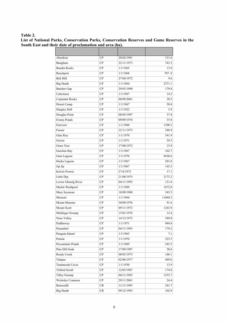
Table 2.List of National Parks, Conservation Parks, Conservation Reserves and Game Reserves in theSouth East and their date of proclamation and area (ha).

Park Name Reserve First Proclaimed Total Area (ha)

Type

Aberdour CP 28/02/1991 131.6

Bangham CP 22/11/1973 743.3

Baudin Rocks CP 1/1/1965

Beachport CP

Belt Hill CP

13.9

1/1/1968 707. 8

27/04/1972

Big Heath CP

Butcher Gap CP

Calectasia CP

Carpenter Rocks CP

Desert Camp CP

Dingley Dell CP

Douglas Point CP

Ewens Ponds CP

Fairview CP

Furner CP

Glen Roy CP

Gower CP

Grass Tree CP

Guichen Bay CP

Gum Lagoon CP

Hacks Lagoon CP

Jip Jip CP

Kelvin Powrie CP

Little Dip CP

Lower Glenelg River CP

Martin Washpool CP

Mary Seymour CP

Messent CP

Mount Monster CP

Mount Scott CP

Mullinger Swamp CP

Nene Valley CP

Padthaway CP

Penambol CP

Penguin Island CP

Penola CP

Piccaninnie Ponds CP

Pine Hill Soak CP

Reedy Creek CP

Talapar CP

Tantanoola Caves CP

Telford Scrub CP

Tilley Swamp CP

Wolseley Common CP

Bernouilli CR

Big Heath CR

9.6

1/1/1964 2371.1

29/03/1990 179.8

1/1/1967 14.2

06/09/2001 30.5

1/1/1967 50.8

1/1/1922 5.9

08/05/1997 37.8

09/09/1976 35.8

1/1/1960 1390.5

22/11/1973 288.9

1/1/1970 541.9

1/1/1971 39.3

17/08/1972 15.9

1/1/1967 102.7

1/1/1970 8430.6

1/1/1967 201.0

1/1/1967 145.5

27/4/1972 17.1

21/08/1975 2173.2

04/11/1993 131.6

1/1/1969 1872.0

18/09/1980 343.5

1/1/1964 11604.3

30/09/1976 91.6

09/11/1972 1263.9

15/01/1976 12.4

14/12/1972 389.0

1/1/1971 984.8

04/11/1993 179.2

1/1/1963 7.1

1/1/1970 225.5

1/1/1969 543.5

17/09/1987 50.6

08/03/1973 146.1

02/06/1977 489.6

1/1/1930 13.9

12/03/1987 174.8

04/11/1993 1535.7

29/11/2001 24.4

11/11/1993 241.7

09/12/1993 102.9

9

NP

NP

NP

Bunbury CR 11/11/1993 1943.6

Canunda CR 11/11/1993 1030. 6

Desert Camp CR 11/11/1993 880.4

Hardings Springs CR 24/4/1997 6.3

Naracoorte Caves CR 02/08/1990 70.7

Woakwine CR 11/11/1993 422.8

Bool Lagoon GR 1/1/1967 3092.1

Bucks Lake GR 1/1/1968 137.9

Lake Robe GR 04/11/1993 404.0

Poocher Swamp GR 14/11/1985 77.1

Canunda 1/1/1959 9273.8

Coorong 1/1/1966 50804.8

Naracoorte Caves 27/04/1972 460.5

Total Area 106,724.0

10

Figure 5.

Environmental Associations (Laut et al. 1977a) overlaying the study area. The numbers

represent Environmental Province, then Environmental Region, followed by the Environmental

Association number.

11

This scientific information is collected to relationship between the fauna and the defined

enhance integrated natural resource habitats,

management and to assist in the conservation • document the biogeography of plant and of South Australia’s biological diversity. animal communities with the information

obtained from the survey, The main aim of the Biological Survey of the • identify characteristic species, communities South East was to conduct both a vegetation and habitats of the South East, and vertebrate survey across the range of • identify potential threats to the region’s habitats comprising the South East and publish biological diversity,the findings in a report. Specific objectives are • summarise findings in a consolidated report. listed below:

Additional objectives associated with the • collate existing information about the flora, National Forest Inventory were also part of the

fauna and their habitats, vegetation survey focus. These objectives • systematically survey the flora and fauna at were to contribute to the;

selected sample sites throughout the study area • completion of a continental scale study of and document the physical characteristics of native forests, these sites, • production of a forest inventory database

• sample the terrestrial invertebrates using suitable for local and regional applications, and standard micro- and macro- pitfall trapping • completion of the forest inventory of South techniques, Australia’s known temperate forests.

• map vegetation associations (floristics and

structure) across the South East at a scale of

1:40,000 ,

• analyse the biological survey database to

determine floristic communities and the

12

CLIMATE

3By D. Hopton

The South East region of South Australia has a region, has an annual rainfall of 581.1 mm while

cool moist climate with long mild dry summers, in the north Keith has an annual rainfall of 470.6

followed by cool wet winters. The Köppen mm (Table 3 and 4). This decrease in annual

classification places this region in the temperate rainfall northward and away from the coast causes

climate zone. Mount Gambier, in the south of the a graduation of Köppen’s classification from Csb

study area, has an annual rainfall of 775.4 mm. In for coastal regions to Cfb for inland regions.

comparison, Naracoorte, in the centre of the

Table 3.

Mean Annual Rainfall for eight South East weather stations.

)Weather Station Mean Annual Rainfall (mm

Keith 470.6

Bordertown 619.0

Padthaway 525.4

Kingston 740.4

Robe 634.1

Naracoorte 581.1

Penola 708.8

Mount Gambier 775.4

Table 4.Mean monthly rainfall (mm) for Keith, Naracoorte and Mount Gambier.

J F M A M J J A S O N D

Month

Keith 18.6 21.0 21.5 34.4 54.0 53.1 55.7 58.9 51.2 44.2 31.8 26.2

Naracoorte 23.7 19.9 26.7 44.1 60.3 73.7 76.1 73.2 64.4 52.1 36.4 30.6

Mount Gambier 32.3 29.0 35.7 63.4 84.0 96.6 107.1 99.8 77.2 63.4 45.9 41.2

The close proximity of the ocean also affects

temperature, restricting the seasonal and Data from the Bureau of Meteorology are presented

diurnal temperature ranges of the coastal zone. for rainfall and temperature for Keith, Naracoorte

The average mean maximum temperature and Mount Gambier to illustrate the climatic change

increases northward and inland. Mount that occurs moving inland and northward (Tables 3-

Gambier has an average mean maximum 5 and Figures 6a-c).

temperature of 19 oC, Naracoorte 20.8

oC and

Keith 22.1 oC (refer to Table 5).

Biological Survey and Monitoring, Science and Conservation Directorate, Department for

Environment and Heritage, PO Box 1047, ADELAIDE SA 5001.

13

3

Table 5.Mean daily maximum temperatures in

oC for Keith, Naracoorte and Mount Gambier.


29.7 29.7 26.9 22.3 18.3 15.4 14.9 16 18.4 21.5 24.5 27.6

27.9 28.6 25.4 21.5 17.4 14.8 14.2 15.4 17.2 20.2 22.8 25.4

24.3 24.8 23.0 19.5 16.5 14.2 13.6 14.7 16.4 18.6 20.6 22.7

Month

Keith

Naracoorte

Mount Gambier

Evaporation is high during the summer. In the

south of the study area the median monthly

rainfall exceeds the mean monthly evaporation

rate for only three months in winter. In the

northern inland areas rainfall exceeds

evaporation for only one or two months

Wind speed and direction for Robe and Mount

Gambier have been published in ‘The

Environments of South Australia – Province 1

South East (Laut et al. 1977a). At Robe, winds

are generally south-westerly to south-easterly

in summer while being more variable in winter

tending to be more from the south-west and

north-west. At Mount Gambier winds are

generally southerly in summer and again more

variable in winter but tending towards

northerly or westerly.

14

a)

0

10

20

30

40

50

60

70

0

5

10

15

20

25

30

35

Rain

fall

(mm

)

Tem

pera

ture

(C

)


Month

b)

c)

0

10

20

30

40

50

60

70

80

0

5

10

15

20

25

30

35

Rain

fall

(mm

)

Tem

pera

ture

(C

)


Month

0

20

40

60

80

100

120

0

5

10

15

20

25

30

Rain

fall

(mm

)

Tem

pera

ture

(C

)


Month

Figure 6.

Mean monthly rainfall and mean monthly temperatures recorded at a) Keith, b)

Naracoorte and c) Mount Gambier.

15

PREVIOUS BIOLOGICAL RESEARCH

By L. M. B. Heard, J. Foulkes, T. Croft and W. Barker

Prior to this study there had been no attempt to

systematically survey the entire South East in a single

study for either vegetation or fauna. Since 1939 a

number of smaller scale surveys have been conducted

that investigated various parts of the area. The

previous biological research is summarised under the

Vegetation and Fauna sections below.

PREVIOUS BIOLOGICAL STUDIES

In terms of understanding the dynamics of the region

and the flora and fauna biologists, are relative

newcomers when compared to the indigenous people

and their knowledge at the time of European

settlement. Aspects of the intimate biological

knowledge that the indigenous people had acquired

over thousands of years in the region are recorded here

in extracts from Angas (1847).

“About this creek [Ross’s Creek] we began to find

various indications of natives; the most remarkable

being wicker work snares for bird-catching, about four

feet high, erected on the flats. Near these snares were

formed small covered places, just large enough for one

person to squat in; the native, concealing himself in

this ambush, with his snaring rod protruded from a

small aperture in the side, imitates the voice of the

birds, and, as they alight upon the wicker work,

dexterously slips the noose around their necks, and

snares them into his retreat.” Angas (1847)

“On these plains [beyond Lacepede Bay] we met with

many tracks of the natives, and their old encampments

were numerous. Heaps of the melliferous cones of the

banksia were lying round these deserted wirlies. The

natives steep the cones in water, which extracts the

honey, and produces a sweet beverage.” Angas (1847)

The use of intricate bird snares in the region and the

use of Banksia marginata flowers to make a sweet

beverage are just some examples of this knowledge.

Pretty et al. (1983) discussed a number of aspects of

Aboriginal life and customs in more detail.

This section focuses on European knowledge gained on

the biological aspects of the region and provides an

indication of the type of work conducted in the study

region. Some more detailed descriptions of previous

work conducted in the study area are presented in the

relevant chapters. .

VEGETATION

Past Botanical Work

While the South East indigenous communities, prior to

European settlement, had developed knowledge of the

local flora over thousands of years European

knowledge of the flora of the South-east has only

developed since the 1840s. This knowledge of the

flora has developed in conjunction with that of

Australian flora, which began initially as a

predominantly European based activity beginning in

the late 1700s, but by the early 1900s was increasingly

(and is now largely) undertaken by Australian

botanists.

Plant collections, in the form of herbarium specimens,

are integral to classifying and describing plants and to

providing an authentic updateable record of their

geographic distribution. Unlike the Far West Coast,

Eyre Peninsula, Spencer Gulf, Gulf St Vincent and

Kangaroo Island, scientific collecting and

documentation of the plants of the South East did not

commence with the coastal explorations of Flinders

and Baudin in 1802, as neither of these parties made

landfalls along the South East coast. Instead plant

collections commenced with settlement of the region,

the first serious collector possibly being John George

Robertson, who, from his base in Portland, where he

settled in 1840, made collections in western Victoria

through to Penola and Rivoli Bay (Kraehenbuehl

1983a, Kraehenbuehl 1986).

From this start, there have been three notable phases of

botanical activity (Barker and Barker 1990). The

initial phase, which lasted until the beginning of the

20th

Century, centred around the activities of Ferdinand

von Mueller (1825-1896) who visited South-east in

1848 (collecting localities included Rivoli Bay and

Lake Alexandrina). Mueller who was initially based in

Adelaide before his move to Melbourne in 1852, was

the first serious resident botanist to publish on the

Australian flora. He published voluminously and also

distributed material globally which enhanced

publication by others. He also encouraged a network

of people around Australia to collect for him. In the

South-east these included his sister Clara Wehl, Dr

L.W. Schulzen, F. Osswald, J.W.T.L. Blandowski, and

Rev. J.E. Tenison-Woods. Others to botanise in the

South East during the later part of Mueller’s influence

included J.G.O. Tepper, a Miss Allen, K. Ward, Miss

N. MacDonald, S.Dixon and Dr R. Brummit. These

people collected for a associate of Mueller’s, Professor

Ralph Tate of the fledgling University of Adelaide.

Tate produced the first "Flora of Extratropical South

Australia" (Tate 1890) and also made collections in the

South East.

The next phase involved the massive contribution of

resident South Australian botanist J.M. Black (1855-

1951) and his associate collectors such as J.B Cleland,

E.C.[and C.D.] Black, E.H. Ising, E. Ashby, A.M.

Ashby, H.W. Andrew, S.A. White, R.S. Rogers: J. M.

Black also documented the flora in his series ‘Flora of

South Australia’ (Black 1908, 1924-26, 1948-52) and

in many scientific publications describing new species

17

and distributional records. Others who made

collections at that time included E.S. Alcock, Mrs E.M.

Petherick, L.D. Williams. Notable collections

underpinning ecological studies by the University of

Adelaide from the 1920s were made by T.G.B. Osborn,

C.M. Eardley, R.L. Crocker, T.B. Paltridge, H.P.C.

Trumble, E.L. Robertson (nee Ashby), R.L. Specht and

D.E. Symon.

Finally, with the establishment of the State Herbarium

of South Australia in the mid 1950s, there was

significant increase in collections by staff and

associated individuals and organisations, and a

publicatons programme of research work and floristic

summaries (e.g. Eichler 1965, Jessop and Toelken

1986, Jessop 1993). Collections in the State

Herbarium from the region now number almost

30,000). Notable resident collectors were Doreen

Hunt, I.B. Wilson (Forest Research Institute, Mt

Gambier) and Kath Alcock.

More detailed information on the contributions made

by these collectors is available in Kraehenbuehl

(1983a, b, 1986).

Past Vegetation or Landscape Studies

The first descriptive information on the landscape and

vegetation of the region was found in accounts by

overlanders who followed Charles Bonney’s

exploratory journey from Victoria to Adelaide in

March 1939, establishing the early stock route between

Melbourne and Adelaide. These overlander accounts

include Charles Bonney (Bonney no date), Joseph

Hawdon and Alfred Mundy in July 1839 (Hawdon

1839), George Hamilton in mid winter 1839 (Hamilton

1880), and Edward and Fortescue Arthur in February

1843 (Arthur and Arthur circa 1844). Providing more

detailed descriptions tied to a more accurately defined

route are the accounts of Angas (1847) and Burr (1845)

from Governor Grey’s 1844 expedition to the region.

With settlement in the area came a more detailed

publication describing the natural landscape of the

region when Rev J.E. Woods produced a volume

focussed on geological observations in the region. In

this publication Woods provided descriptions of the

landscapes and the dominant soils, landforms and

vegetation communities based on his observations as

he travelled around the region (Woods 1862).

Further advancements to the knowledge and

distribution of native vegetation communities within

the region were made by a variety of authors over the

last century. In the 1930s – 1940s these included

studies of sphagnum bogs near Lake Leake (Crocker

and Eardley 1939) and an ecological study of the

vegetation of Eight Mile Creek by Eardley (1943).

Major studies attempting to define and map the

principal vegetation associations and to research the

edaphic and other environmental factors influencing

these communities came particularly through the

detailed work of Crocker (1944) for the Lower South

East; Coaldrake (1951) for part of the Upper South

East (Ninety-Mile Plain); Specht (1951) for the Tatiara

(Bordertown) district; Litchfield (1956) in the

Coonalpyn Downs area (Upper South East); and Specht

(1957a-b) for the Dark Island heath (Ninety-Mile

Plain). The detailed mapping and vegetation

association descriptions provided by Crocker (1944)

and Coaldrake (1951) were particularly relevant and

useful in completing the regional vegetation mapping

resulting from the South East survey work.

Studies by Taylor (1933), Blackburn et al. (1953),

Blackburn (1959a-b) and Blackburn (1965), though

focussed specifically on soils, for various parts of the

study region also included observations and

commentary on the relationships between native

vegetation and soils thereby adding to the vegetation

knowledge base. Research into grasslands by Tiver

and Crocker (1951) provided some background on the

native grasslands or grassy ecosystems for the

Kalangadoo and Naracoorte areas and how these had

been affected by pasture development activities.

Specht (1972) drew on all these sources to produce a

broadscale regional map for the South East and to

provide detailed descriptions of the major vegetation

communities within the state.

In the mid 1970s research by Dodson concentrated on

using pollen analysis of lake sediments to describe the

vegetation history of Lake Leake (Dodson 1974,

Dodson 1975b) and the Mt Gambier region (Dodson

1975a). Dobson’s work for the Mt Gambier region

using sediments from Brownes Lake revealed that the

native vegetation around that area consisted mainly of

open grasslands with some sparse woody vegetation

(Dobson 1975a). Dobson and Wilson (1975) also

investigated the vegetation history and soil

development of Marshes Swamp. Other studies in the

1970s included the Nature Conservation Societies

(NCSSA) survey work on the Southern Coorong and

Lower Younghusband Peninsula. In terms of

vegetation work this study involved mapping the

vegetation formations for the area and running

transects across the area to study the vegetation

associations in more detail (Gilbertson and Foale

1977).

Responding to the removal of native vegetation

through agricultural development and drainage,

Mowling and Barritt (1980) undertook the first work

across the whole region as defined by this study. They

mapped the location of the large (>100 ha) remnants

and describing these areas in terms of their landforms

and vegetation types. Barritt (1982) added to this work

with a supplementary report on 16 islands of vegetation

in the Upper South East (eastern half), providing brief

descriptions of the landforms and vegetation within

these areas. Another significant addition to the

knowledge of specific blocks in the South East came

through work by Paton (1983) on Big Heath

Conservation Park. This report was commissioned by

18

the South Eastern Wetlands Committee to document

the vegetation of the park and predict the likely impact

of proposed hydrological changes on the flora and

fauna. Paton undertook survey work, that built on the

previous survey and mapping work conducted by the

NCSSA in 1969, producing detailed mapping and an

analysis of the vegetation quadrat data. In the western

half of the Upper South East the proposed development

of a lignite mine at Kingston prompted a detailed

examination of the vegetation for the development area

by Lange and Nicolson (1982) for the Environmental

Impact Assessment report (Kinhill Stearns 1982).

With the growing awareness of the importance of

wetlands in the region and the impact of hydrological

changes, specialist studies were undertaken that

focussed on wetland areas. Reviewing the wetland

resources of the area the South East Wetland

Committee (1983) report provided summaries on 78

wetland areas across the a region. This report provided

brief descriptions of the vegetation communities at

each of these locations, their conservation value and

any recommendations for future management. More

detailed investigations of the wetlands of the Baker

Range and Marcollat watercourse was undertaken by

Atkins (1988).

Increasing concern by Local Councils in the lower

South East prompted specialist studies into the

distribution and management of Coastal Wattle (Acacia

longifolia var. sophorae) along roadsides (Cohen 1981,

Stevens 1983).

During the 1980’s, further vegetation mapping was

carried out by the Remote Sensing Applications

Branch, Department of Environment and Planning

undertaking vegetation survey and mapping projects

for the Coorong National Park and Game Reserve

(Remote Sensing Applications Branch 1982a) and the

Beachport 1:50,000 map-sheet (Remote Sensing

Applications Branch 1982b). This detail mapping used

interpretation of photo mosaics in conjunction with

ground and aerial survey. This mapping was an

important step towards the regional mapping and

provided a significant resource to the National Parks

and Wildlife Service as did the work by Davies (1982)

to assist in park management planning. The report by

Davies (1982) on the major plant associations in South

Australia was pivotal in assessing the conservation

significance of the major plant associations and

providing vegetation community descriptions for parks

and reserves. While not all park management plans

had vegetation maps produced, vegetation community

information was compiled in these plans providing a

useful addition of specific block based vegetation

information to expand the regional vegetation

knowledge base.

Sparrow (1991) undertook additional research into the

vegetation communities and the environmental

influences for the region. A significant part of

Sparrow’s work was a multivariate analysis of floristic

data as part of his larger geo-botanical study of the

remnant natural vegetation of temperate South

Australia. This was the first regional multivariate

analysis for the region. Information from that analysis

was used when reviewing the analysis undertaken as

part of this South East Biological Survey vegetation

analysis.

The proposals for surface and ground water drainage

schemes as part of the Upper South East Dryland

Salinity and Flood Management Plan (Upper South

East Dryland Salinity and Flood Management Plan

Steering Committee 1993) resulted in a number of

small park-based or specific wetland area biological

surveys conducted during the 1990s. These surveys to

assess the likely biological impacts of the proposed

drains or drainage options included Messent

Conservation Park (Owens et al. 1995); Deep Swamp

(Stewart 1996); Tilley Swamp (Stewart et al. 1998);

Bunbury Conservation Reserve and Stoneleigh Park

Heritage Agreement (Stewart et al. 1998); Gum

Lagoon Conservation Park (Davies 2000); and West

Avenue Range (Stewart et al. 2002). These special

purpose surveys used the standard sampling techniques

as used on the regional surveys but involved a more

intense sampling. They contributed specific park or

area vegetation site data, analysis of this data and

detailed vegetation mapping which either has been

incorporated into the regional mapping or requires

incorporation. Following on from these specific

surveys and in response to the construction of surface

water or groundwater drains in these areas, specific

programs monitoring the health of vegetation have

been implemented. These monitoring programs focus

on the health of Melaleuca heaths along transects at

intervals away from and parallel to the drains. The

results are reported in Telfer et al. (2000) and Milne

and Squire (2001) for the Tilley Swamp area, and

Stewart (2001) and Milne et al. (2001) for the Deep

Swamp area.

Prompted by the release of drainage waters under the

new drainage scheme other vegetation studies were

also implemented. These included investigation into

the location and condition of fresh water soaks along

the southern lagoon of the Coorong (Bickerton and

Winter 2001). In addition a survey to monitor any

significant changes in health of the Leptospermum

lanigerum community and associated species for the

Henry Creek area was also established (Carpenter and

Squire 2002).

Apart from targeted biological and monitoring surveys

other research in the early 1990s, also focussed on the

effects of salinity and rising watertables. Loan (1993)

investigated the health of native vegetation relating to

rising ground water and salinity levels in the Upper

South East. Similarly Webb (1993), investigated the

health of low-lying native vegetation (mainly

Melaleuca halmaturorum and Melaleuca brevifolia)

affected by rising water tables in the Bunbury Taunta

area. More specific and detailed research into the

19

water use strategy of Melaleuca halmaturorum in these make to overall vegetation cover in the region and their

saline swamps was undertaken by Mensforth (1996). conservation status (Bickerton et al. 2002).

Away from the salinity and drainage issues of the FAUNA

Upper South East other biological surveys including Prior to this survey there had been no large-scale

detailed vegetation work were undertaken. Stokes general vertebrate surveys of the South East. Several

(1996) concentrated on the significant Box and Buloke biological surveys of vertebrates had been carried out

grassy woodlands and vegetation associated with the in the survey region prior to the 1997 South East

heavy clay soils of the Bordertown – Frances area. Biological Survey. These included the South East

This study provided a comprehensive systematic Coast (1980’s), South East Fire Study (NCS) (1994),

survey of these vegetation communities building on Messent Conservation Park (1994), Gum Lagoon

earlier work particularly by Specht (1951). The Nature Conservation Park (NCS) (1995, 1996), SE Box and

Conservation Society in conjunction with the SA Buloke Woodlands (1995), Deep Swamp (1996) and

Farmers Federation undertook a study investigating the Tilley Swamp (1996). The Bunbury Conservation

possible use of fire as a management tool for remnant Reserve survey was carried out in December 1997 after

vegetation in the Upper South East. The study looked the main South East survey work had been completed.

at 14 areas (13 areas north of Bordertown and 1 area to

the south west), undertaking extensive flora survey as Several of these surveys have concentrated on specific

well as the collection of fuel accumulation data and areas in response to proposed changes in land

information on plant species responses to fire (Nature management. There have also been a few small-scale

Conservation Society of SA 2000). Stewart et al. surveys targeting specific threatened species such as,

(2001) undertook a survey of the Lake Hawdon area in Swamp Antechinus (Antechinus minimus) Swamp

response to the need for detailed biological information Skink (Egernia coventryi) and Geocrinia laevis. Much

for the area, which is characterised by large expanses of the work on the ecology of individual species found

of sedgelands. Eight vegetation quadrats were in the South East has been carried out in the eastern

surveyed and six vegetation communities were states where populations of these species are more

recognised (Stewart et al. 2001). widespread and easier to detect.

Croft and Carpenter (1998) compiled biological data South Australian Museum records showed a high

for the region, summarising the major vegetation types number of mammal, reptile and amphibian specimens

provided details of the distribution of the communities, distributed throughout the South East region prior to

the landforms on which they occur, their condition, the 1997 South East Survey. The specimens came

understorey features, special habitat features, from a variety of sources including a large number of

management issues and conservation priorities. This random collections from individuals in the region.

resource document provided the essential background Amphibians have been well represented in these

for the South East Biodiversity Plan (Croft et al. 1999), collections making up approximately 40% of

which guides biodiversity work within the region. specimens, however it was not until the 1960s that

specific attention was paid to the frog fauna of the

Recent work continues to focus on the gaps in South East (Thompson and Tyler 1983). Substantial

knowledge within the region. Specific studies cover fauna collections have come from the SA Herpetology

threatened species and threatened communities or more Group, Field Naturalist Society of SA Mammal Club,

broadscale issues such as scattered tree clearance. Roseworthy Agricultural College (now Adelaide

Craig and Pritchard (2001) investigated three orchid University), Salisbury College (now University of SA),

species (Caladenia richardsiorum, Caladenia calcicola NPWSA Rangers, Museum collection trips and

and Pterostylis tenuissima) and compiled recovery Department for Environment and Heritage and Nature

plans; and Cutten and Squire (2002) have investigated Conservation Society of SA (NCSSA) Biological

the distribution of Senecio macrocarpus within the surveys.

sedgeland areas of Messent Conservation Park. In

terms of threatened communities Bachmann (2002) One other major source of data for frogs in the South

provides detailed information on the Leptospermum East is the South Australian Frog Census. This census

lanigerum and Gahnia trifida areas visited and is coordinated by the Environment Protection

assessed in the Lower South East over the 3 year Silky Authority and has been run each September since 1994

Tea-tree and Cutting Grass Wetland Rehabilitation (Walker 2002). The census aims to provide a

project. ‘snapshot’ of frog populations based upon the

collection of frog recordings from as many different

With regard to scattered trees, clearance assessment locations as possible over a one-week period. The

guidelines have been developed based on a point South East is well represented and each year valuable

scoring system to assist the Native Vegetation Council data is recorded on the presence and location of

with its legislative requirements (Cutten and Hodder different species.

2001). In addition, a mapping project has begun that

aims to assess the contribution that scattered trees The biological surveys conducted throughout the

region have been invaluable in documenting the fauna

20

of the region and have helped define the distributions

and habitat preferences of many species. The survey

reports have also drawn attention to some of the more

threatened species that has helped secure funding for

work that is more intensive. Despite this, there is still

little known about the distribution and ecology of many

species in the region, and with continuing changes in

land management practises some of the more

apparently threatened species may be disappearing

from areas before they have even been detected.

Invertebrates have been surveyed inadequately in the

region, with the distribution of most families poorly

known. ‘The Natural History of the South East’

handbook (Tyler et al. 1983), provided summaries of

knowledge of a number of groups; arachnids (Lee

1983), butterflies (Fisher 1983), myriapods, insects and

allied forms (Gross 1983). The freshwater invertebrates

are better known than terrestrial invertebrates (Zeidler

1983), however they are not systematically recorded as

part of the Biological Survey of South Australia, and as

a result are not included in this report.

Fish are not systematically recorded as part of the

Biological Survey of South Australia, and as a result

are not reported in detail on this report. Recent survey

work by Hammer (2002), however, recorded fourteen

native species, including three species of national and

six species of state conservation significance, and

described the South East as a biodiversity ‘hotspot’ for

freshwater fishes. Five introduced species were

detected. Five additional native species and a range of

introduced species (exotic and native to other regions

of Australia) were recorded previously or presumed to

occur in the area (Hammer 2002).

The following photographs (Figures 7-15) provide a

visual sample of some of the landscapes from the South

East.

Figure 7. Typical eucalypt Stringybark Woodland with Bracken (Pteridium esculentum) understorey near Penola. Photo: A. Robinson.

21

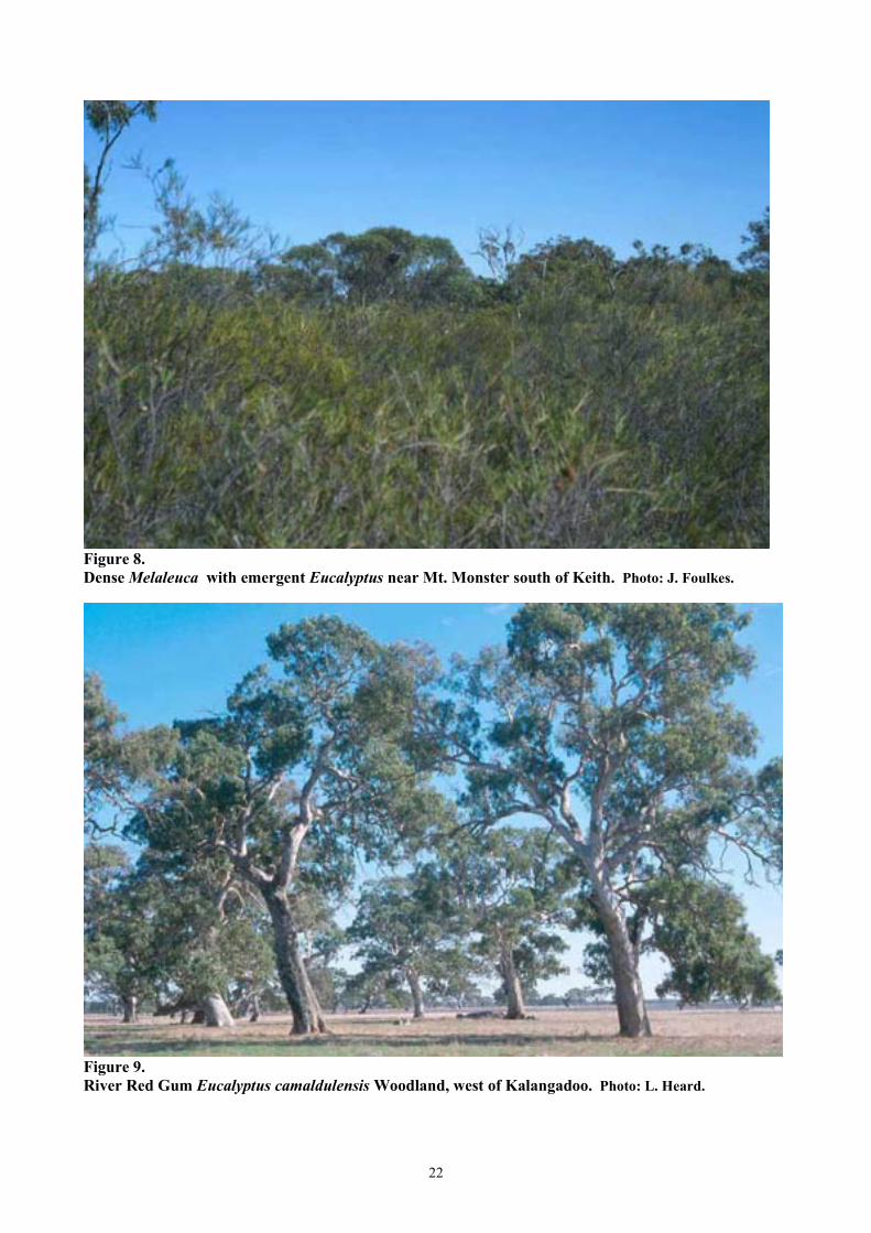
Figure 8.Dense Melaleuca with emergent Eucalyptus near Mt. Monster south of Keith. Photo: J. Foulkes.

Figure 9.River Red Gum Eucalyptus camaldulensis Woodland, west of Kalangadoo. Photo: L. Heard.

22

Figure 10.Swamp in Honans Scrub near Glencoe in the Lower South East. Photo: J. Foulkes.

Figure 11.Granite outcrop near Willalooka in the Upper South East. Photo: T. Croft.

23

Figure 12.Jaffray Swamp northeast of Kingston. Photo: G. Carpenter.

Figure 13.Stringybark Woodland with Xanthorrhoea understorey, in The Bluff NFR, east of Tantanoola. Photo:L. Heard.

24

Figure 14.SA Blue Gum Woodland (Eucalyptus leucoxylon). Photo: A. Robinson.

Figure 15.Cutting Grass Swamp in Marshes Swamp NFR with Stringybark Woodland in the background. Photo:D. Kraehenbuehl.

25

4


GEOLOGY AND GEOMORPHOLOGY By M.C. Benbow

INTRODUCTION

The geological and geomorphological setting of the

South East region of South Australia is in marked

contrast to that of the northern part of the State such as is

exemplified by the Sandy and Stony Deserts (e.g.

Benbow 1999, 2000). The southern continental margin is

a region in which very thick Mesozoic and Tertiary

sediments accumulated, a result of the dismemberment of

Gondwana, which led to the final separation of Australia

from Antarctica (Krieg 1995, Morton 1995). It is

because of the region's proximity to the coast after the

formation of these continents, that there have been

successive transgressions of the sea, resulting in a marine

sedimentary record that includes the fossiliferous

limestones of the Murray and Gambier Basins. Fossils

have enabled these sediments to be placed within a

temporal framework and thus allow better insight into the

region's geological history.

During the Pliocene, quartz sands deposited during a

major episode of transgression and regression gave rise

to the formation of a large coastal strand plain on which

157 coastal dunes have been preserved (e.g. Kotsonis

1995 and references therein). This plain is mainly

preserved to the north of the study area. A legacy of the

rapid fluctuations of sea level and of gradual uplift during

the Quaternary, is the unique succession of calcarenitic

strandlines or coastal dunes that are a major feature of the

region (Sprigg 1952 1979). These have been linked to

the Earth's orbital parameters (i.e. eccentricity and

ellipticity). The Younghusband Peninsula and The

Coorong are the modern analogues of the Quaternary

coastal barriers and backbarrier lagoons.

The South East is also unique in the State, because of the

record in the Mt Gambier region, of recent volcanic

activity (Sheard 1983, 1995). The southern part of the

region is also important as a karst province Twidale et al.

1983, Grimes et al. 1995). This contains a Quaternary

record of the changes of climate and biota and of

prehistoric man's occupation. In fact the Naracoorte

caves collectively contain a fossil record of ~ 500 000

years, a record that is more diverse than anywhere else on

the mainland (Moriarty et al. 2000, R.T. Wells, personal

communication, 2000). The Tertiary and Quaternary

limestones that the karst has developed in, are important

as unconfined aquifers of good quality water that has

various economic uses in a region that is intensely

farmed. The sediments of the Mesozoic Otway Basin

contain economic reserves of gas, including carbon

dioxide, and possibly of oil (Morton and Drexel 1995).

Previous geological compilations of the region are

included in various works of the Geological Survey of

South Australia, for example the 'handbooks' of Parkin

(1958), Glaessner and Parkin, (1969) and more recently

that of Drexel and Preiss (1995 and references therein).

More specific studies include that of the Otway Basin by

Wopfner and Douglas (1971) and the Murray Basin by

Brown and Stephenson (1991). The South East was the

first area in South Australia to be mapped at 1:250 000

scale by the Geological Survey and includes the map

sheets of PENOLA, NARACOORTE and PINAROO

(Sprigg 1951, Rockow 1969, 1971, Rogers 1980, 1981).

More regional 1:500 000 scale-maps of the entire South

East have been published with explanatory notes

providing a useful and updated overview and synthesis

(e.g. Rogers 1995). Previous studies include those of

Sprigg (1952, 1979), Cook et al. (1977) and Schwebel

(1983) on the stranded coastal dunes of the Mt Gambier

coastal plain. Sheard (1983, 1995) published studies on

the volcanoes of the Mt Gambier region and of Twidale

et al. (1983) on other landforms including granite forms,

karst and lunettes. More recently, Grimes et al. (1995

and references therein) have documented aspects of the

karst. Work on the cave history and their deposits and

fossil remains continues (e.g. Moriarty et al. 2000).

GEOLOGY

Early Palaeozoic Stansbury Basin and Delamerian

granites

The oldest rocks of the region are Cambrian

metasediments, which only occur in the subsurface

having been intersected in drillholes (Figures 17,18 and

19). They are unnamed equivalents of the Cambrian

Kanmantoo Group of the Kanmantoo Trough, that

outcrop in the eastern Mt Lofty Ranges and on northern

Kangaroo Island for example. Gravestock (1995, cf

Rogers 1995)) regarded the Cambrian rocks of the South

East as belonging to the Stansbury Basin whilst the

occurrences within the Kanmantoo Trough have been

regarded as being part of the Adelaide Geosyncline (e.g.

see Preiss 1993). Lithologies include marble and

metamorphosed mudstone, sandstone, conglomerate and

volcanics. These Kanmantoo Group equivalents that are

extensive in the subsurface, range in depth from 100-

200m in the north, to 1000-5000m in the south, as in the

Mt Gambier region. There is some evidence in the north

of still older Cambrian rocks that include basic volcanics

and metasediments that pre-date the Kanmantoo Group

equivalents. The Cambrian metasediments were

deposited within a deep basin that formed because of

rifting within older basement rocks, when Australia

formed part of a much larger continental mass that lay in

an equatorial position.

Longlat Enterprises, PO Box 458 KAPUNDA SA 5373 27

4

There are small and scattered outcrops of a range of acid

to basic intrusive rock types, including granite,

adamellite, dacite, rhyolite, basalt and gabbro. These are

the surface expression of the Padthaway Ridge, an

uplifted basement feature that lies to the west of the

Dukes Highway and more or less parallels the coast

(Figures 17 and 18). These rocks are Ordovician in age

and intruded the older Cambrian rocks, at the same time

that they were deformed and metamorphosed during the

Delamerian Orogeny.

Late Palaeozoic Troubridge Basin

This basin formed sub-parallel to the current coast,

during the Late Carboniferous and Early Permian

approximately 300 million years ago when Australia

formed the eastern part of the super-continent of

Gondwana (Figures 16 and 18). A large icecap formed

over a large part of the super-continent, as high as 1 km

in Australia, as it was located in high southern latitudes

and as this was a time of more marked equator-polar

temperature gradients. The mechanism driving these

cooler global climates is believed to be processes within

the Earth, when there were large continental masses (the

icehouse climate mode of Fischer (1984) and Veevers

(1990)). In the study area, glacial sediments of the Cape

Jervis Formation, belonging to the Troubridge Basin,

occur in scattered pockets and become more extensive

toward Adelaide in the north. North-westerly directions

of ice movement are indicated by the scoured pavements

at Hallet Cove and Inman Valley, both in the Basin.

There is very little documented record of this time from

the South East, most of it comes from the more extensive

and outcropping occurrences of the Basin in the Fleurieu

Peninsula region. In the study area there are drillhole

intersections of the Cape Jervis Formation, believed to be

preserved in glacial valleys. Rogers (1995) describes

these sediments as being diamictites, which contain clasts

of granite and metasediment reworked from the Early

Palaeozoic rocks.

Figure 16.Geological and tectonic setting of the South East of South Australia. (After Rogers (1995)).

There are also marine, foraminifera-bearing sediments,including sandstones and mudstones that were depositedduring a major transgression that occurred after thewaning of glaciation, as has also been recorded in theinland Carboniferous-Permian basins.

Mesozoic Otway BasinDuring the Mesozoic the super-continent of Gondwana,located in high southern latitudes, started to fragment due

to internal movements within the Earth. Initial rifting

between Australia and Antarctica commenced in the

Jurassic some 175 million years ago and gave rise to the

formation of a series of basins of the Australian Southern

Rift System, including the Otway Basin which straddles

the South Australian and Victorian border (Stagg et al. 1990, Krieg 1995, Figures 16, 17 and 18). As

fragmentation of Gondwana took place, there were

increases in volcanic activity, which resulted in distinctly

28

higher levels of carbon dioxide in the atmosphere.

Global climates became generally warmer (the

greenhouse climate mode of Fischer (1984) and Veevers

(1990), but because of the continent's high southern

position climate was generally moist and cool if not cold

(e.g. Frakes and Francis 1988, Krieg 1995).

The northern Basin limit, which is orientated

approximately east-west, lies just south of the Padthaway

Ridge in the Kingston-Naracoorte region and the Basin is

made up of a number of similarly orientated troughs or

sub-basins and intervening basement highs. A large part

of the Basin lies offshore in the Southern Ocean. A

considerable thickness of sediment, some 3-5 km in fact,

accumulated in the Basin during the Mesozoic. During

the rift phase of sedimentation in the Early Cretaceous,

much of the sediment was derived from

contemporaneous, inland and offshore, volcanic sources,

including the Wisanger Basalt of Kangaroo Island. They

were deposited in lacustrine and fluvial environments and

belong to the lithostratigraphic unit named the Otway

Supergroup (e.g. Morton 1995).

Toward the end of the Mesozoic, in the Late Cretaceous

around 95 million years ago, crustal extension reached

the point that enabled rupture, the formation of new

ocean crust and drifting and led to the development of the

Southern Ocean (Veevers 1986, Stagg et al. 1990).

During this post-rift phase of separation, the nature of the

sediments deposited in the Otway Basin changed and the

focus of deposition moved toward the southwest.

Quartz-rich sediments, including mudstones and

sandstones of the Sherbrook Group, were deposited in

fluvial and deltaic environments. Apparently, a large and

deep saline lake formed the focus of deposition, with

deltas rimming the lake on both the mainland and

Antarctic sides. Marine influence at this time is minor.

The 1 km thick, black and carbonaceous, Belfast

Mudstone, indicates either a time of maximum basin

subsidence or a eustatic sea level peak. Much of the

sediment was deposited in the offshore Voluta Trough

where most, contemporaneous, basin subsidence

occurred. A feature of the Otway Basin, is the large

number of faults that accommodated the rapid deposition

of a thick pile of sediment (Figures 16 & 18).

29

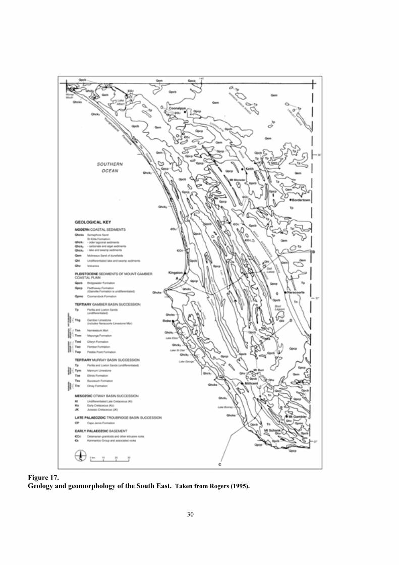
Figure 17.Geology and geomorphology of the South East. Taken from Rogers (1995).

30

Figure 18.Cross sections through the Otway Basin in the South East of South Australia. Taken from Rogers (1995).

31

Figure 19.Cross sections through the Mount Gambier coastal plain in the South East of South Australia. Taken fromRogers (1995).

Cainozoic Gambier and Murray Basins

As Australia began it's northward migration toward the

equator, a series of Cainozoic basins formed in the region

of the Australian Southern Rift System and beyond

(Figures 17 and 19). The Gambier Basin is not included

in the Otway Basin, previously being referred to as the

Gambier Embayment of the Otway Basin (Wopfner and

Douglas 1971). This is because of the change that took

place in the Late Cretaceous and Palaeocene, in structure

and tectonic style, namely from that of an active rift zone

32

to that of a passive, drifting continental margin (Smith et al. 1995). The pocket of Cainozoic sediments is, in

contrast to the Mesozoic sediments, relatively fault-free

and flat lying, the upper part of which is a carbonate

platform. The thickness of Cainozoic sediments

increases from 50-200m near the Basin's inland margin to

around 750m offshore. The boundary of the Gambier

Basin with the much larger Murray Basin to the north is

somewhat arbitrarily placed along the Padthaway Ridge,

near Kingston and east to southeast across to Naracoorte.

In the Naracoorte area, the margin coincides

approximately with the Kanawinka Fault, which also

marks the limit of Otway Basin sediments with very

shallow Palaeozoic sediments on the northeast side

(compare Smith et al. (1995) and Rogers (1995)).

The Murray Basin, in contrast to the Gambier Basin is a

very large, circular shaped, epicratonic basin, in which

similar and equivalent sediments were deposited. The

succession is thinner, with maximum thicknesses being

of the order of 600m, and the access to the sea was

generally more restricted, apart from the time of

maximum transgression in the Late Oligocene to

Miocene.

Sedimentation commenced in the Gambier Basin at the

end of the Palaeocene, 55 million years ago with the

terrigenous clastics of the Wangerrip Group (Figures 17

& 18). Thicknesses are up to ~ 800 m. Sediments

include mudstones and sands that are in part

carbonaceous, and that may contain glauconite. There

are also coal seams in the Dilwyn Formation.

Environments of deposition included rivers, deltas and

inter-distributary bays. The occurrence of the restricted

marine Cyclammina facies (which includes planktonic

foraminifera) indicates the opening of the seaway of the

Southern Ocean. The base of the Group is marked by the

~40m thick Pebble Point Formation notable for it's oolitic

grits, which Gravestock et al. (1986) interpreted as

implying little input of detrital sediment in

interdistributary bay settings.

To the north, in the southern margin of the Murray Basin,

deposition of equivalent sediments, namely the lower

part of the Renmark Group, that is, the Olney Formation

commenced somewhat later in the Eocene. Sediments

include carbonaceous mudstone and sandstone as well as

lignite and these were deposited in non-marine, that is

floodplain, fluvial, swamp and lake environments.

After a brief hiatus, sedimentation in the Gambier Basin

recommenced with a major transgression of the sea, in

the Middle Eocene, ~46 million years ago. The seaway

had opened sufficiently for the deposition of limestone’s

for the first time for well over 400 million years and thus

commenced the construction of a marine carbonate

platform. Sediments deposited in the Middle to Late

Eocene are referred to as the Nirranda Group (Figures 16

& 18). The base of the Group is marked by a

transgressive, thin (ie ~ 10m) quartz grit, that contains

minor amounts of marine fossils and that may have been

deposited as a beach barrier. As the sea deepened,

fossiliferous and glauconitic calcareous mud of the

overlying Narrawaturk Marl was deposited offshore, in

low energy environments, that is, below storm-wave

base. The thickness of this unit is generally less than

15m. To the north, on the landward side of the

Padthaway Ridge, non-marine sediments of the Olney

Formation continued to be deposited in the Murray

Basin. The laterally equivalent Buccleuch Formation

that includes bryozoan limestone and glauconitic marl

indicates some marine influence in the western part of the

Basin in the Late Eocene.

In the Gambier Basin the Narrawaturk Marl passes

upwards and laterally into the Gambier Limestone,

reflecting more open marine environments with better

circulation and less input of terrigenous clastic sediment

from onshore. Deposition of this formation commenced

in the Late Eocene in the offshore, ~40 million years ago

and later near the Basin's margin in the Early Oligocene,

that is ~33 million years ago (Figures 17 & 18). Age of

the top of the formation ranges up into the Middle

Miocene. Formation thickness increases from around

50m onshore to in excess of 400 m offshore, toward the

platform margin. The Gambier Limestone outcrop is

limited to the Mt Gambier region and an upfaulted block

near Naracoorte.

Lithology is predominantly a bryozoan calcarenite or

limestone, with textures including wackestone,

packstone, and grainstone. The Gambier Limestone has

been subdivided into several members based on

differences in lithology. The Greenways Member in the

lower part includes marl and is glauconitic at the base

making it quite similar to the Narrawaturk Marl. The

overlying Camelback Member is a bryozoan carbonate,

while the Green Point Member is, as the name denotes,

distinctive because of it's colour, but it is also distinctly

cherty in nature. In the northern part of the Basin there is

the ~6m thick Naracoorte Limestone Member, a coarser

grained limestone that contains the remains of molluscs

and echinoids. It has also been described as being rubbly

because of subsequent partial dissolution.

33

Figure 20. Stratigraphic column for the Cainozoic of the Gambier and Murray Basins. Taken from Alley (1995).

In the Murray Basin during the Oligocene, there was an

increasing marine influence as can be seen by the fossil

content in the upper part of the Olney Formation. As

deposition of this formation became more restricted, the

Ettrick Formation became the dominant sequence in the

Late Oligocene in the southwest of the Basin, indicating

a transgression at this time. The latter is a sequence that

includes silt and fine-grained sand, and calcareous mud

or marl that is both glauconitic and fossiliferous. As

marine influence increased in the Late Oligocene and

Early Miocene, the Ettrick Formation passed upwards,

particularly in the southwest part of the Basin, into the

more open marine Mannum Limestone. This unit, that is

distinctly sandy in the lower part, is comprised of

bryozoan limestone and marl.

Deposition ceased in both the Gambier and Murray

Basins in the Middle Miocene, around 12-15 million

years ago. The cause of non-deposition is believed to be

due to uplift of the continent's southern margin and the

fact that there was a drop in sea levels globally. Thus

there ensued a time of erosion and weathering, including

the development of karst on the Gambier Limestone (see

below). Terra rosa soils are commonly associated

(Blackburn 1983).

A new phase of sedimentation commenced in both basins

at the end of the Miocene and Early Pliocene, around 5

million years ago. In contrast to the marine carbonates

and muds of the preceding major episode of deposition,

quartz-rich sands, namely the Loxton Sand and Parilla

Sand and their equivalents, became the dominant

lithology of the Pliocene (Figure 17, 18 & 19). Belperio

and Bluck (1990) referred to these sands collectively as

the 'Pliocene Sands' as they are difficult to differentiate

and they form an onlap-offlap sequence. There is

extensive outcropping and sub-cropping Pliocene sands

preserved north of Naracoorte where thickness is

typically 30-50m. These sands are no longer present

beneath the Quaternary coastal plain to southwest, most

likely due to marine erosion.

The Loxton Sand is generally fine grained and it is

calcareous due to it's detrital component of fossil-derived

grains. The formation is also mica bearing. The basal or

lower sands are marine and were deposited offshore to

near shore on a shallow shelf. The upper part is

comprised of beach and aeolian sands, deposited as a

series of beach ridges were formed during regression,

that is as the coastal plain prograded toward the

southwest (see below). Preserved beach ridges on this

strand plain include the Lawloit and Marmon Jabuk

Ranges east of Coonalpyn, in the northeast corner of the

map (Figure 17; see below). The sands of the most

southwesterly range are distinctly calcareous, containing

numerous fragments of broken shell remains.

In contrast, the Parilla Sand is ferruginous quartz sand

that is clayey and fine to medium grained. These

sediments form part of a regressive sequence, that is, they

were deposited as the sea retreated toward the southwest,

by rivers and in lakes. There is also an aeolian or wind-

blown component. Belperio and Bluck (1990) believe

that there may be remnant transgressive dunes preserved.

Much of the unit was derived from reworking of the

older Loxton Sand. However since the strandlines are

evident over so much of the region outcropping fluvial

sands must be very restricted. Sometime in the Late

Pliocene after deposition, there was extensive weathering

resulting in both ferruginisation and silicification,

referred to as the Karoonda Palaeosol (e.g. Firman 1973).

Deposition in the Quaternary commenced with the

Coomandook Formation that was deposited because of a

major transgression in the Early Pleistocene (Figures 17,

19 & 20). The formation occurs over the extent of the

coastal plain, as far inland as the Marmon Jabuk and

West Naracoorte Ranges, and is now largely buried

beneath the younger Quaternary sediments. Average

thickness is 25m or less with a maximum known

thickness of around 75m. The exposures southeast of Mt

Gambier, are comprised of beach sediments that are both

gravelly and shelly. Most of the formation is comprised

of clay, sandstone and fossiliferous limestone that were

deposited in near shore, marine environments. The

source of the formation is believed to have been older

sediments that were reworked. The palaeogeography for

the time of maximum Early Pleistocene transgression

indicates bays and granite headlands (Belperio and Bluck

1990, Figure 20).

34

Figure 21.Cross sections through the Quaternary MtGambier coastal plain. Taken from Cook et al.(1977), Williams et al. (1988) and Huntley et al. (1993).

As the sea retreated after maximum transgression, a

unique series of parallel beach ridges or coastal dunes

were formed, marking temporary stillstands on the Mt

Gambier coastal plain (Sprigg 1952, 1979, see below,

Figures 20 & 21). The Bridgewater Formation is the

name given to the beach and aeolian calcarenites that

were deposited at this time. A number of facies have

been recognised in the calcarenites and these can be

viewed along the crosscutting road and drain exposures

(Belperio 1995). The near shore, transgressive subtidal

facies, is coarse-grained lime sand with skeletal

fragments derived from shells, coralline algae and

foraminifera. Beach calcarenites tend to be a little fine

grained and quartz sand bearing. Up to 3m thick, these

sediments can be traced into the core of the coastal dunes

from their southwest side. The overlying transgressive

dune facies forms the bulk of the formation being which

can be up to at least 75 thick as in the West Naracoorte

Range. These calcarenites are well sorted and fine to

medium grained and the skeletal grains are rounded.

Large scale cross bedding which can be prominent, dips

inland. The source of the calcarenites is from the

continental shelf. Soils developed on the calcarenites of

the ranges include podzols, humic podzols (i.e. grey

sands in the upper part of the profile) and red brown

sand-capped terra rosa (Blackburn 1983)

As each beach ridge was successively built, lake and

lagoonal, muds, dolomite, limestone and sand of the

Padthaway Formation were deposited on their landward

side (Figures 2, 5 & 6). The back-barrier lagoonal

sediments of the Padthaway Formation are poorly sorted,

muddy calcarenites, which contain shells including the

bivalves Andara, Katelysia and Ostrea. The commonly

overlying lacustrine facies include 1-2m thick calcareous

and dolomite mudstone and interbedded green mud

clayey sand. Fossil remains of molluscs, ostracods and

foraminifera may be present in the mudstones, indicative

of fresh to brackish lake waters. Much of the

outcropping sediment is mud and marl, on which dark

grey, to black soils (i.e. rendzinas) have developed

(Blackburn 1983, P.A. Rogers, personal communication,

2000). Where grey sands occur in the upper part of

markedly differentiated profiles, solodic and solodized

solonetz soils have developed. These sediments were

deposited both during coastal dune construction but also

at other times as the coastal plain developed. Thickness

of this formation is typically 10-15m. The name

Glanville Formation is given for the equivalent sediments

that were deposited during the last interglacial, around

100,000 to 120,000 years ago. They have been mapped

south of Kingston between the Reedy Creek and

Woakwine Ranges.

On the coastal plain, outcrops of Bridgewater and

Padthaway Formations alternate successively over the

coastal plain. When the oldest of the stranded coastal

dunes were formed, namely the Coonalpyn and East

Naracoorte Ranges, there were wide embayments with

granite headlands at Mt Boothby and Willalooka. The

orientation of both the Pliocene and Pleistocene coastal

dunes indicates prevailing westerly winds not unlike

those of today.

The coastal dunes formed during the Pleistocene

interglacial peaks, as these were times of globally high

sea level, which was related to the melting of the polar

ice caps. Thus they can be linked to the

ellipticity/eccentricity orbital parameters of the Earth

(Figure 5; Sprigg 1952, 1979, Cook et al. 1977,

Schwebel 1983, Huntley et al. 1993, Williams et al. 1988). Sea level fluctuated by as much as 130m during

the glacial/interglacial cycles. The ridges are preserved

because the region has undergone very gentle uplift

35

Figure 22.Depositional environments of The Coorong. After Belperio (1995).

during the Quaternary, of around 0.07mm per year

(Belperio 1995). The coalescence of the dunes toward

the northwest is indicative of minimal uplift in that

region. Near Mt Schank, the Burleigh Range that

formed during the penultimate interglacial around

200,000 years ago, is distinctly higher than it's

equivalents to the northwest, indicating significant

uplift in this recently volcanically active region. The

oldest coastal ranges, namely the Coonalpyn and West

Naracoorte Ranges (~870,000 years old) being

preserved inland and the youngest, such as the

Woakwine Range (~100,000 years old) formed near the

modern coast. Dating by various means, including

thermoluminescence techniques, of the sediments of

the ranges has been carried out. (e.g. Cook et al. 1977,

Idnurm and Cook 1980, Schwebel 1883, Huntley et al.

1993) supporting the model of Sprigg (1952, 1979).

Calcretes or calcium carbonate-rich palaeosols have

formed within the calcarenites of the Bridgewater

Formation. There may be associated calcified remains

of plant and insect material and these formed a number

of times. For example, the Formation has been divided

into upper and lower members, being separated by the

indurated Ripon Calcrete and capped by the Bakara

Calcrete (e.g. Firman 1973). Their formation is

indicative of arid to semiarid climate conditions,

perhaps of the Pleistocene glacial episodes (Estaban

and Klappa 1983).

After the last glacial episode peaked 18 000 years ago,

sea levels rose to their present level around 6,000 years

ago and the Holocene sediments of the coast were

deposited (Figure 17). Collectively referred to as the

St Kilda Formation they are the modern analogues of

the Pleistocene sediments that form the Mt Gambier

coastal plain. These include the beach and aeolian

sands of the Semaphore Sand of the present day coastal

barrier, namely the ~ 180 km long Younghusband

Peninsula, that fronts the sea. There is a general

increase in the carbonate content and a decrease in

grain size of both beach and dune sands, in a direction

away from the River Murray Mouth, toward the

southeast (e.g. Belperio 1995). Also included in the

coastal deposits are the flint pebble and cobble

sediments of the Port MacDonnell area and the aeolian,

foredune sands of Guichen and Rivoli Bays.

There are a number of lithological facies, that were and

continue to be, deposited behind the coastal barriers, in

the shallow waters of the narrow Coorong and lagoons

and lakes (Figure 22). There are relict sediments,

including shelly muds, that were deposited earlier in

the Holocene, between the Coorong and Lake Bonney,

the Murray mouth and elsewhere. They are relict

because of minor uplift. In The Coorong sediments

'consist of bioclastic magnesium calcite and aragonite

sand and peletal mud derived from molluscs, ostrocods

and foraminifera (Brown 1960)' (Belperio 1995, p235).

In the ephemeral and more saline southern Coorong

waters, and some of the lakes elsewhere, including

Bool Lagoon and Lake Hawdon, mudstones, dolomitic

mudstones and algal deposits continue to be formed.

South of Salt Creek on the east side of The Coorong

there are a number of lakes in which a range of

carbonate types are being currently precipitated,

including aragonite, dolomite and magnesite (e.g. von

der Borch and Loch 1979). There are also coarser

grained, clastic carbonates in the Coorong and

elsewhere and peat is being formed in the Port

MacDonnell area. The life and sedimentary facies of

the seasonally hypersaline lakes are described in the

work of a number of authors (see Belperio 1995).

Aeolian sands of the dunefield in the northern part of

the South East were deposited during the Late

36

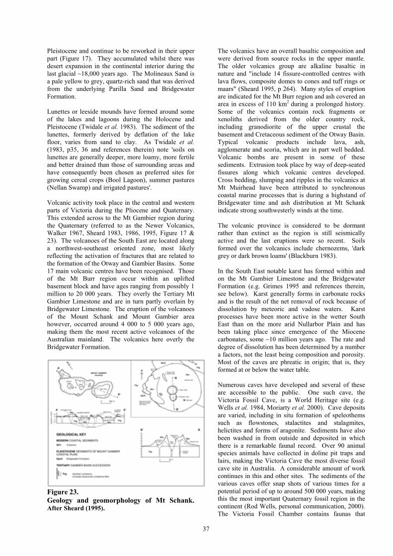
Pleistocene and continue to be reworked in their upper

part (Figure 17). They accumulated whilst there was

desert expansion in the continental interior during the

last glacial ~18,000 years ago. The Molineaux Sand is

a pale yellow to grey, quartz-rich sand that was derived

from the underlying Parilla Sand and Bridgewater

Formation.

Lunettes or leeside mounds have formed around some

of the lakes and lagoons during the Holocene and

Pleistocene (Twidale et al. 1983). The sediment of the

lunettes, formerly derived by deflation of the lake

floor, varies from sand to clay. As Twidale et al. (1983, p35, 36 and references therein) note 'soils on

lunettes are generally deeper, more loamy, more fertile

and better drained than those of surrounding areas and

have consequently been chosen as preferred sites for

growing cereal crops (Bool Lagoon), summer pastures

(Nellan Swamp) and irrigated pastures'.

Volcanic activity took place in the central and western

parts of Victoria during the Pliocene and Quaternary.

This extended across to the Mt Gambier region during

the Quaternary (referred to as the Newer Volcanics,

Walker 1967, Sheard 1983, 1986, 1995, Figure 17 &

23). The volcanoes of the South East are located along

a northwest-southeast oriented zone, most likely

reflecting the activation of fractures that are related to

the formation of the Otway and Gambier Basins. Some

17 main volcanic centres have been recognised. Those

of the Mt Burr region occur within an uplifted

basement block and have ages ranging from possibly 1

million to 20 000 years. They overly the Tertiary Mt

Gambier Limestone and are in turn partly overlain by

Bridgewater Limestone. The eruption of the volcanoes

of the Mount Schank and Mount Gambier area

however, occurred around 4 000 to 5 000 years ago,

making them the most recent active volcanoes of the

Australian mainland. The volcanics here overly the

Bridgewater Formation.

Figure 23.Geology and geomorphology of Mt Schank.After Sheard (1995).

37

The volcanics have an overall basaltic composition and

were derived from source rocks in the upper mantle.

The older volcanics group are alkaline basaltic in

nature and "include 14 fissure-controlled centres with

lava flows, composite domes to cones and tuff rings or

maars" (Sheard 1995, p 264). Many styles of eruption

are indicated for the Mt Burr region and ash covered an

area in excess of 110 km2

during a prolonged history.

Some of the volcanics contain rock fragments or

xenoliths derived from the older country rock,

including granodiorite of the upper crustal the

basement and Cretaceous sediment of the Otway Basin.

Typical volcanic products include lava, ash,

agglomerate and scoria, which are in part well bedded.

Volcanic bombs are present in some of these

sediments. Extrusion took place by way of deep-seated

fissures along which volcanic centres developed.

Cross bedding, slumping and ripples in the volcanics at

Mt Muirhead have been attributed to synchronous

coastal marine processes that is during a highstand of

Bridgewater time and ash distribution at Mt Schank

indicate strong southwesterly winds at the time.

The volcanic province is considered to be dormant

rather than extinct as the region is still seismically

active and the last eruptions were so recent. Soils

formed over the volcanics include chernozems, 'dark

grey or dark brown loams' (Blackburn 1983).

In the South East notable karst has formed within and

on the Mt Gambier Limestone and the Bridgewater

Formation (e.g. Grimes 1995 and references therein,

see below). Karst generally forms in carbonate rocks

and is the result of the net removal of rock because of

dissolution by meteoric and vadose waters. Karst

processes have been more active in the wetter South

East than on the more arid Nullarbor Plain and has

been taking place since emergence of the Miocene

carbonates, some ~10 million years ago. The rate and

degree of dissolution has been determined by a number

a factors, not the least being composition and porosity.

Most of the caves are phreatic in origin; that is, they

formed at or below the water table.

Numerous caves have developed and several of these

are accessible to the public. One such cave, the

Victoria Fossil Cave, is a World Heritage site (e.g.

Wells et al. 1984, Moriarty et al. 2000). Cave deposits

are varied, including in situ formation of speleothems

such as flowstones, stalactites and stalagmites,

helictites and forms of aragonite. Sediments have also

been washed in from outside and deposited in which

there is a remarkable faunal record. Over 90 animal

species animals have collected in doline pit traps and

lairs, making the Victoria Cave the most diverse fossil

cave site in Australia. A considerable amount of work

continues in this and other sites. The sediments of the

various caves offer snap shots of various times for a

potential period of up to around 500 000 years, making

this the most important Quaternary fossil region in the

continent (Rod Wells, personal communication, 2000).

The Victoria Fossil Chamber contains faunas that

accumulated during the full range of a number of

glacial/interglacial cycles (Moriarty et al. 2000).

ECONOMIC GEOLOGY

Petroleum

There has been a long exploration history since algal

remains (coorongite), found along the coast in the

1890's, was believed to be oil-derived. Robe 1

drillhole was sunk in 1915. Katnook 1 drilled in 1987

intersected the first economic gas find in the Basin and

oil was subsequently discovered soon after.

Hydrocarbons continue to be explored in the sediments

of the Otway Basin with use being made of better

quality seismic data that is now available. Economic

quantities of gas occur in at least three reservoirs,

particularly the Pretty Hill Formation, but there are also

occurrences in fractured basement rocks. The

reservoirs occur within deeper trough or sub basin

regions between parallel, northwest-southeast oriented

basement highs and traps include both stratigraphic and

structural types. A number of source rocks are

indicated (Morton 1995, Morton and Drexel 1995).

Kalangadoo 1 and Caroline 1 wells have intersected

CO2 fluids at depth in the volcanic province of the

South East, with the latter having produced commercial

quantities. The origin of the CO2 is volcanic with a

primitive mantle source (e.g. Wopfner and Thornton

1971, Chivas et al. 1987).

Coal

Thin coal seams occur in several Cretaceous

formations of the Otway Basin succession but are of

possible economic value. The younger Eocene lignites

of the Gambier Basin, northeast of Kingston, have been

actively explored by Western Mining Corporation.

Here there is a trough ~30 km long and 5km wide

which contains lignite (~1 000 million tonnes) with

cumulative thicknesses of up to eight or so meters.

Depths of overburden of 40-75m, high moisture, ash

and salt content, together make the deposit

uneconomic. The lignite is similar in character to other

Tertiary lignites of the State.

Groundwater

There are significant quantities of good quality ground

water in the South East but as there is intense land use

in the region, there are considerable pressures on this

resource, not the least being the problems of pollution

and dry land salination (Waterhouse 1977). There are

two main aquifers, the upper one being unconfined

whilst the lower one is confined. The former is the

more important of the two and occurs in the Cainozoic

limestones (e.g. Bridgewater Formation and Mt

Gambier Limestone). Water movement in this aquifer

is from the east to west and at a rate of ~100m per

annum. The water table depth is close to surface over

much of the region, particularly between the coastal

dunes and recharge is primarily by direct infiltration.

There are springs south of Mt Burr in an arcuate line to

the coast, and along or near the coast south of Mt

Gambier, at which water discharge takes place. Water

salinity increases toward the northwest from ~500

mg/L to over 1 4000 mg/L.

The confined aquifer occurs within the older and

deeper, Eocene clastic sediments. The Kingston area

relies more heavily on the aquifer where salinity is

<1500mg/L. There is an increase in salinity toward the

northwest where the sands thin and the overlying and

inter-tonguing muds become more prominent.

Building materials

The Gambier Limestone (Camelback Member) has

been used since 1844 for the construction of houses

and other buildings. The quarries include that of Marte

which produce over 11 000 tonnes per year, making

them the largest dimension stone producers in

Australia.

GEOMORPHOLOGY

The South East region lies within the Central-Eastern

Lowlands, a large low-lying region of Australia (David

and Browne 1950, Gentilli and Brown 1963) as can be

seen on the DTM of Australia of Moore and Simpson

(1982). It can be very broadly divided into two major

regions, the low lying Quaternary Mount Gambier

coastal plain and the more elevated and older, that is

Pliocene, partially dissected and mantled coastal strand

plain to the east of the Kanawinka Fault and

Escarpment. The latter was referred to as the Pinnaroo

Block in the PINNAROO area to the north and as the

Naracoorte Plateau in the south (Firman 1973, Twidale

et al. 1983). In the Mt Burr-Mount Gambier region

there is also the local and distinctly more elevated

region that is occupied by the Quaternary volcanoes.

Pliocene coastal strand plain

A digital terrain model of the South East generated

from AUSLIG data by PIRSA, shows this area to have

elevations that are typically over 100m and up to 184m

as in the Mt Shaugh area on the Lawloit Range (Figure

17). The southwest margin drops away to join the Mt

Gambier coastal plain at the position of the oldest of

the Pleistocene coastal dunes (see below). The

variation in relief is attributable to subsequent erosion

by water and wind, gentle tectonic warping and the

plains original variation in relief, notably the presence

of superimposed coastal dunes. Thus, this elevated

region had its origins as a stranded coastal dune-

mantled plain. Kotsonis (1995, 1999) has recognised

157 stranded dunes on it's surface. Several of these are

prominent in the northeast, namely the Marmon-Jabuk

Range and the Lawloit Range. Less prominent are the

relict ridges recently identified east of Keith and in the

region east of Naracoorte, there are parallel ridges, the

Joanna and Hynman Ranges (e.g. Rogers 1997).

The Pliocene coastal dunes, which are constructed of

quartz sands, are gently arcuate and have an overall

northwest-southeast orientation as can be seen on

NOAH-AVVR and LANDSAT satellite imagery.

They are narrow, that is generally less than 2-3 km

wide and stand up to 30m above the intervening plain.

38

The southwest margin of the Marmon Jabuk Range is

marked by a scarp that is believed to have resulted

from marine erosion during the Early Pleistocene

(Rogers 1980, Figure 17). The two subdued (i.e. 10m

high) ranges east of Naracoorte have resulted from the

erosion of the Mt Gambier Limestone and thus they are

not constructional features. They may mark Pliocene

or Early Pleistocene shorelines where erosion took

place. Rogers (1997) notes the occurrence of relict

Early Pleistocene Coomandook Formation on one of

them.

Quaternary Mount Gambier coastal strand plain

The Mount Gambier coastal plain is unique because of

the succession of superimposed strand lines of Middle

to Late Pleistocene age, first documented by Sprigg

(1951, 1952, Figures 17 & 21). They are comprised of

the calcarenites of the Bridgewater Formation (see

above). The coastal plain extends from the Murray

River mouth region toward the South East into

Victoria. Width of the plain is ~80-95 km and the

elevation gradually increases from sea level to around

50-60m adjacent to the West Naracoorte and

Coonalpyn Ranges that lie close to the plain's eastern

margin. Elevation also decreases toward the northwest,

although the region constrained by the Coonalpyn and

The Black Ranges is slightly higher.

There are 13 named ranges between Robe and

Naracoorte (Figure 19). Individual ranges can be

traced for up to 140 km (e.g. Reedy Creek Range).

They are straight to slightly curved and are oriented

parallel to the modern coast, having an overall

northwest-southeast orientation. Toward the

northwest, southwest of the West Naracoorte Range

and The Black Range, the ranges coalesce; reflecting

the fact that uplift in that direction has been rather

limited (e.g. Belperio 1995). Thus, in the Big

Desolation-Policeman Point region there is a broad

region, 15-25 km wide, that is parallel to the coast and

that stands 15-25m above the adjacent plain. Average

width of most of the dunes in contrast, and height, is

~1-3km and ~15m respectively. The highest coastal

dunes lie adjacent to the Kanawinka Fault. Thus the

Naracoorte West Range lies up to ~75 m above the

coastal plain. Presumably, erosion has diminished the

ranges height since their formation. The range

morphology, including arcuate forms that reflect

palaeo-embayments and headlands. The most obvious

example is the Coonalpyn Range, which has granite

highs at each end that were once headlands.

Toward the southern end of the Mount Gambier coastal

plain, in the region that is slightly more elevated, the

coastal dunes in the region of Mount Burr and Mt

Gambier, are more dismembered or less well defined

and in part show some evidence for coalescence. It is

likely that this region did not undergo the same, even,

gentle uplift as occurred to the immediate north and

northwest. The isolated, linear to irregular shaped,

highs that occur southwest of Naracoorte are likely to

be relict fragments of coastal dunes.

At the coast, there is the parallel, modern or Holocene,

coastal dune that arose as a result of the current

interglacial and eustatic sea-level rise to the current

position 6 000 years ago. This is the currently active

Younghusband Peninsula, which is the latest of the

Quaternary coastal dunes of the Mt Gambier coastal

plain to have formed. It extends from Lacepede Bay to

the Murray River Mouth, ~180km to the northwest.

The average width and height are 0.75-1.0 km and < 45

m respectively. The Peninsula faces onto the

Encounter and Lacepede Bays and Southern Ocean.

Vegetation free (ie mobile) and vegetation-fixed

transgressive dune complexes occur on the peninsula,

which are up to 40m above the beach and include both

parabolic and transverse dune forms and have

associated blowouts or depressions. Locally exposed

there is evidence of aboriginal occupation including

middens of cockleshells. On the east side of The

Coorong, there are also a parallel series of low

discontinuous foredunes with scattered elongate playa

lakes.

To the south there are a series of bays or compartments

that may have eroded the Bridgewater Formation that

forms the modern headlands or capes as at Cape Jaffa

and Cape Dombey (Figure 17). Numerous arcuate

shaped and parallel beach ridges are apparent in the

strand plains of the compartments, reflecting Holocene

progradation of the coast. Thus, Guichen Bay contains

over 80 foredune ridges that stand up to 10m above the

present beach (Thom et al. 1981). This part of the

coastline, as does much of the southern margin of

Australia, is under the influence of the prevailing

westerlies and the high-energy swell regime of the

Southern Ocean.

Modern dunefield

Draped over part of the coastal plain and Pinnaroo

Block landforms, more so in the north and in the

Bordertown area, are low aeolian buildups or sand

sheets that formed at the end of the Pleistocene (Figure

17). They are the southern "outposts" of the extensive

Mallee dunefield. In contrast with the region to the

immediate north, as in the Pinnaroo area (e.g. see

Rogers 1980) there are very few duneforms

recognisable. They include both linear and parabolic

forms northeast of Keith. The older linear dunes that

occur to the north are not apparent in the South East,

indicating that either they are masked by the modern

sheets and dunes or that the older dunefield limits were

more restricted.

The Coorong, lakes, lagoons, lunettes and drainage

The narrow ~ 130km long, shallow Coorong, lies along

much of the landward margin of Younghusband

Peninsula and is the modern analogue of marine

influenced lagoons that once lay behind the previously

active, successively older, coastal dunes (Figure 17).

Waters become progressively more saline toward the

south, as circulation becomes more restricted and

where shallow, interconnected basins have developed.

Water is derived from a number of sources, namely the

39

Murray River, the Southern Ocean, groundwater and

run-off and consequently, water level and salinity

varies seasonally.

To the south of The Coorong, there are also a series of

shallow, behind barrier lakes, namely Lakes Eliza,

George and Bonney. They are groundwater discharge

lakes that do not have a direct link with the ocean and

lake-salinity varies enormously. There are also

shallow lakes or lagoons in between some of the

ranges, such as Bool Lagoon and Salt Lakes.

Drainage is generally poor and the expression of

modern drainage is generally limited in the South East

region of the State. In fact, drainage is so poor in part

of the region that drains have been excavated to gain

access to the sea. There are creeks draining off the

older coastal plain in a general southwesterly direction,

terminating in the lakes and lagoons between the West

Naracoorte and Harper Ranges. The coastal dunes of

the Quaternary strand plain have the effect of limiting

surface drainage and of allowing water to collect and

pond in the intervening mud floored flats, as noted for

example by Twidale et al. (1983). In addition, between

the coastal dunes, the groundwater table outcrops

locally. Thus, numerous small and often linear shallow

mud flats, swamps and lagoons have formed between

the dunes, being more evident during times of winter

rainfall.

Twidale et al. (1983) describe the fact that many of the

lakes have low lying lunettes developed on their lee

side, that is particularly so on their eastern or

southeastern margin. A good example is the lunette of

the Bool Lagoon, which stands up to 20 m above the

lake floor, is 3km long and ~0.3 km wide. Lunettes

may be only centimetres high to >30 m as at Lochaber

Swamp. Their cross sectional form is markedly

asymmetric, with the lake side portion being distinctly

steeper, where wind erosion takes place. It is not

understood why some lakes of a particular region have

these lee side mounds whilst some others do not.

Karst

In the flat, low lying, karstic province of the South

East, there is a range of dissolution features and

collapse structures, namely dolines, cenotes, uvalas and

caves (Twidale et al. 1983, Grimes et al.1995, Figure

17). Spectacular karst has developed, particularly in

the Naracoorte and Mt Gambier regions. There are a

number of caves open to the public, namely

Tantanoola, 'Little Blue Lake', Victoria Fossil,

Umpherston, Engelbrecht and Mitchell Caves and Cave

Gardens. The karst of the Mt Gambier Limestone is

much more extensive than that of the Bridgewater

Formation, having developed over a much longer

period. The karst reaches greater depths toward the

coast because of the increasing thickness of the

limestones in that direction and the lower sea levels

and thus water tables, during the Pleistocene glacial

periods, the water table is commonly intersected in the

caves. There are features such 'Little Blue Lake', 'Hells

Hole' and 'The Shaft' which have attracted divers.

Many of the caves of the Naracoorte area 'include

doline to horizontal passage solution and collapse

structures' (Sheard and Smith 1995, p259). Cave form

is partly determined by jointing in the limestones.

As Twidale et al. (1983, p 30, see their figure 9 taken

after Marker (1975) state 'the underlying limestones

have imposed some of their characteristics on the relief

forms' where there is a thin cover of sediment. Thus

enclosed depressions are common, be they single or

coalesced sinkholes. Extensive exposed karst occurs

south and west of Mt Gambier. Here the Miocene

limestones display pavements and solution cups or

hummocky karst surface features with karren

sculpturing. Along the creeks draining off the old

elevated plain east of Naracoorte there are associated

shallow circular swamps that may be partially infilled

dolines. Swamp dolines or uvulas and circular shallow

depressions occur in the Bool Lagoon and Penola

regions and around the margin of Dismal Swamp

region. Deep funnel dolines have formed on the

margins of elevated terrain such as west of the

Kanawincka Escarpment and the volcanic terrain as

near Glencoe. Along the Gambier Lineament, possibly

the surface expression of the Tartwaup Fault there is a

string of elongated and deep dolines.

Where the Mt Gambier Limestone has been locally

eroded, or where there is a thick cover of younger

sediment, there is no obvious surface expression. The

Bridgewater Formation karst features include minor

caves along the coast, clay pot karst, and pavements

with karren and 'flatteners'.

Granite landforms

There are outcrops of Ordovician granites of the

Padthaway Ridge which display typical granite

weathering landforms (Figures 17, 18 & 19). Many of

these would have been islands, archipelagos and

shallow shoals during the various transgressions of the

Cainozoic and thus may be quite old. They stand out

above the plain up to heights of at least 20 m. They

have been described by Twidale et al. (1983, and

references therein). Joint pattern and spacing is

regarded as being generally more important than

lithologic variation in determining the shape of granite

landform. Differential weathering related to joint

patterns can give rise to inselbergs or steep sided

residual hills surrounded by boulder fields at plain

level.

Angular blocks have formed on resistant quartz

keratophyres as at Bin Bin and Easter Rock. Some

granite hills, such as those at Jip Jip and Crotty Nob,

are mantled by rounded-boulders. A few boulders may

rest on the top of gentle rises. The large radius domes

east of Richardson Rocks and at the Granites have a

scatter of boulders. Domes may have few or no

scattered boulders. The large residual boulders, as at

Richardson Rocks, can have slightly flared sides or

may be whaleback in form as exposed on the beach

40

near Kingston. Larger granite hills may display many

joints and compartments of fresher rock surrounded by

a skin of weathered rock. Flat plateau and depressions

have formed in places where weathering has occurred

at the base of cornerstones of granite compartments.

Old plain levels can be reconstructed based on these

features. Twidale et al. (1983) argue that the stepped

larger hills of Kongai and Tolmer Rocks indicate

multiple episodes of lowering of the landsurface.

During the various Cainozoic transgressions, tide and

wave action is believed to have eroded the domains of

weathered granite and thus sped up the process of

boulder formation rather than having been important in

determining shape.

Volcanic terrain

In the region around Millicent and Mt Gambier there

are preserved volcanic cones of Quaternary age

(Figures 17 & 23). Walker (1967) and Sheard (1983)

have characterised the type of volcanic centres as

composite, ash-cone, maar (explosion crater), scoria

dome and flow. Height above the surrounding plains

ranges from 50-168m. Mt Burr, a composite volcanic

centre, is at 240.5 m AHD, the highest of the cones. In

the older volcanic region of Mt Burr area there are at

least 15 volcanic centres, many of which are

recognised by the occurrence of cracks in the ground

that are the surface expression of deep fissures. Here,

there are apparently three main, parallel alignments of

these centres. The asymmetry of the some of the older

centres, such as Mt Muirhead and The Bluff, is

apparently due to aeolian and marine erosion that took

place during times of Late Pleistocene high sea levels.

Both of the southeastern volcanoes are complex maar-

cone structures and formed because of explosive

volcanicity. Mount Schank is an ash-mantled volcano

that has a main crater, a maar on the southern side and

a buried cone on the northern side. The cone is less

than 1 km in diameter and it stands 70-80m high above

the adjacent plain. Small scoria cones lie in line on the

northwestern flank. The craters at Mt Gambier are

large and open the result of the 'influx of abundant

near-surface ground water into the active vents and

conduits' thereby giving rise to steam-induced volcanic

explosion (Sheard 1983, p9). The Blue Lake of Mount

Gambier is one of a number of fresh water lakes that

have formed or mark a series of craters that have an ~

northwest-southeast alignment over a length of ~3.5

km. Remnant cone height is up to at least 130m above

the adjacent plains.

Lange (1983) has described the broad outlines of the

region's original endemic flora, referring to the earlier

work, particularly that of Crocker (1944) and

Blackburn (1964). A section across the Mt Gambier

coastal plain north of Kingston is instructive and

believed to have wider relevance. There is a distinct

correlation between coastal range and plain geology

and vegetation. The exceptions to this broad pattern is

the flora of the aeolian sand plains, the volcanic

province and the 'fen or freshwater alkaline peat

swamp' (Lange 1983, p101).

41

Historical Vegetation Communities 1

By T. Croft

INTRODUCTION

The map in the back pocket of this report shows the

pre-European vegetation communities across the South

East mapped and reconstructed from existing remnants,

previous literature records, soil maps and early

exploration and land survey records. Here details of

the vegetation communities mapped are compared with

literature references over time to place the current

survey in an historical context.

The historical data summarised here take their

structural classification from the SA Vegetation

Structural Formation categories (Appendix VII), which

were derived from Specht (1972) and Muir (1977).

Generally the taxonomy and nomenclature follows

Jessop (1993) as updated by the SA Flora database

2001. The following communities are listed in the

structural formation order (largest lifeform to smallest)

according to the SA Vegetation Structural Formations.

Where two or more vegetation types occur in the same

structural category then these are listed alphabetically.

Where references to soil types are made, based on

literature sources, these are followed with current

Australian Soil Classification terminology, in brackets,

according to Isbell (1996).

The South East is fortunate in having a number of

historical sources for natural history information,

thanks to early settler and traveller accounts from the

nineteenth century, and Government reports of the mid

twentieth century. These have given us some idea of

the appearance of the region prior to artificial drainage

and subsequent agricultural development of the region.

Most of the early accounts are of the sub-coastal areas,

which gave easier access and good feed for horses.

Joseph Hawdon, one of the overlanders pioneering the

stock route between Melbourne and Adelaide wrote

“… it appears that the whole country from the Glenelg

[River] to this point on the Murray is one bed of

limestone alternately covered with sand, swamp, and

strips of alluvial deposit covered with grass and

sheoak” (Hawdon 1840).

In the mid nineteenth century, Government surveyors

described the South East as “…very peculiar, no large

river exists and there are no high mountains to form a

watershed and force the drainage by a strong fall into

any particular channel. The consequence of this is a

number of lakes, lagoons, and swamps which in winter

are of considerable depth and in summer, by

evaporation and soakage are nearly dry” (Hanson,

Parliamentary Papers 1863). Due to this unique

situation, the South East developed the complex

mosaic of plant communities, described below.

FOREST ASSOCIATIONS

In South Australia, open-forests and low open-forests

are largely restricted to the Mount Lofty Ranges,

Southern Flinders Ranges, western Kangaroo Island,

Koppio Hills of southern Eyre Peninsula and the South

East. They occur most extensively occur in the South

East (Specht 1972).

Crocker (1944) described three types of dry sclerophyll

forests in the South East, each characterised by an

abundance of sclerophyllous shrubs and undershrubs.

These forests reach their maximum development in the

Mount Burr Range.

Eucalyptus arenacea/baxteri (Stringybark) Open

Forest

Early European residents and travellers through the

South East noted the generally sandy ridges to be

thickly timbered with stringybark (Burr 1845, Woods

1862), which at times were stunted (Hawdon 1840).

Crocker (1944) considered Eucalyptus

baxteri/arenacea and Eucalyptus obliqua to form two

distinctly different plant communities in the South East

of South Australia. Early literature referred only to E.

baxteri, however subsequently there has been a split,

with E. baxteri known to occur in the southern wetter

areas (around Mt Gambier) and E. arenacea in the

northern drier areas (around Keith – Bordertown).

There appears to be intergrades of these two species in

the area between these extremes (M. O’Leary, pers.

comm.). For the purposes of this section, E.

arenacea/baxteri will be used. Eucalyptus

arenacea/baxteri Open Forest is a widespread

association, although more prevalent in the south of the

region. It predominates on the sandy ranges with an

understorey typically dominated by Pteridium

esculentum, and sporadically tall shrubs and small trees

such as Banksia marginata, Acacia melanoxylon,

Bursaria spinosa and Acacia mearnsii (Crocker 1944).

Early literature referred only to Eucalyptus baxteri

however subsequently there has been a split, with E.

baxteri known to occur in the southern wetter areas

(around Mt Gambier) and E. arenacea in the northern

drier areas (around Keith – Bordertown). In the

intervening area between these to extremes there

appears to be intergrades between these two species

(pers. comm. M. O’Leary, Plant Biodiversity Centre).

For the purposes of this section Eucalyptus

arenacea/baxteri will be used where the references had

previously used E. baxteri.

1 Biological Survey and Monitoring, SA Department for Environment and Heritage, GPO Box 1047 ADELAIDE SA

5001 43

Eucalyptus viminalis ssp. cygnetensis (Rough-barked

Manna Gum) - Eucalyptus arenacea/baxteri (dune

stringybark) Open Forest

Eucalyptus viminalis ssp. cygnetensis - Eucalyptus

arenacea/baxteri Open Forest is described by Crocker

(1944) as dominating most of the Nangwarry area

where the sand is shallower and the habitat is wetter.

In this community, understorey shrubs were noted to be

more diverse, and include Acacia melanoxylon, A.

mearnsii, Leptospermum myrsinoides, L. continentale,

Banksia marginata, Hibbertia species and Pteridium

esculentum.

Eucalyptus obliqua (Messmate Stringybark) Open

Forest

This association is limited to the Lower South East

where it occurs on deeper red clay (terra rossa) soils

(Petrocalcic, Red Dermosol); transition soils at the

edge of some basaltic hills; and shallow sandy soils

over limestone on the ranges and higher country

(Crocker 1944). It covered a smaller area of the South

East than E. arenacea/baxteri Open Forest. The

understorey was noted to be more open comprising

sclerophyllous shrubs such as Acacia species, and with

generally lesser cover of P. esculentum (Crocker 1944).

Eucalyptus willisii ssp. willisii (Willis’ Peppermint)

Low Open Forest

Eucalyptus willisii ssp. willisii Low Open Forest is

limited to the Lower South East from Compton in the

south to nearly Callendale in the north. In this region it

is located in small sandy depressions of the range

country. It never formed widespread areas, but

occurred in small, scattered suitable sites, usually over

a dense wet shrubland understorey of L. continentale,

Gahnia clarkei and G. radula. It was not a plant

community noted in earlier works.

WOODLAND ASSOCIATIONS

The woodlands of the most of the South East have been

described as savannah communities with

predominantly herbaceous and grassy understorey

(Wood 1937, Crocker 1944). In South Australia, the

savannah woodlands are found on southern Eyre

Peninsula, central Yorke Peninsula, southern Flinders

Ranges, Mid North, Mount Lofty Ranges, limited areas

of Kangaroo Island and the South East (Specht 1972).

In the South East, the savannah woodlands were an

important, distinctive feature occurring over a large

part of the region.

Eucalyptus camaldulensis var. camaldulensis (River

Red Gum) Woodland

River Red Gum formed extensive woodlands through a

large part of the region, particularly in the Lower South

East. In the Upper South East, this woodland

community is more restricted to localised areas along

water courses (e.g. creeks) and fringing swamps

(Specht 1951). It is an association that has been greatly

modified due to the artificial drainage system and

grazing by domestic stock since European settlement

(Crocker 1944). The ground understorey was primarily

dominated by grasses, sedges and rushes, but has

subsequently been replaced by clovers, perennial rye-

grass, phalaris and other introduced pasture species

(Crocker 1944).

Eucalyptus fasciculosa (Pink Gum) Woodland

Eucalyptus fasciculosa woodland is predominantly

found in the Upper South East. Here it occurs on

sandier soils of lower fertility and water retaining

ability (Specht 1951). It was also noted to occur on the

lower slopes of the ranges and adjacent strips of the

interdunal plains, fringing freshwater swamps or on

higher dunes in saline swamps (Litchfield 1956).

Specht (1951) recognised the community as E.

fasciculosa – Xanthorrhoea caespitosa on the “Laffer

sands” (Petrocalcic, Brown Chromosol) as part of the

“desert” community complex of the “Ninety-Mile

Plain”. The understorey comprised a variety of

sclerophyllous shrubs, including Acacia myrtifolia var.

myrtifolia, Hibbertia species, Hakea species, L.

myrsinoides and X. caespitosa. However, on loam

soils, the community occurred as distinct savannah

woodland over native Danthonia and Stipa grasses or

sedges (Litchfield 1956).

In the Lower South East, the community becomes less

frequent, but occurred as far south as County Robe on

better loamy soils, with the trees capable of growing

much larger (Crocker 1944). Like some areas of the

Upper South East, it formed distinct savannah

woodland over Danthonia and Stipa species grasses.

Eucalyptus largiflorens (River Box) Woodland

Eucalyptus largiflorens Woodland has a limited

distribution in the South East. It is restricted to the

Upper South East in the vicinity of the Tatiara Creek

floodplain from the Victorian border to Bordertown.

However, the community becomes more prevalent and

extensive east of the border in the Wimmera district of

western Victoria. This community is considered to be

confined to swampy areas with alkaline, heavy-

textured grey soils with a distinct “crabhole” or gilgai

characteristic, mostly drying out in summer (Specht

1951).

The community is typically of a grassy woodland, with

the understorey composed of grass and herbaceous

species, including Brachycome basaltica var. gracilis,

Calocephalus citreus, Carex inversa var. inversa,

Danthonia duttoniana, D. linkii var. fulva, D. setacea

var. setacea and Eryngium vesiculosum.

Eucalyptus leucoxylon ssp. (South Australian Blue

Gum) Woodland

Eucalyptus leucoxylon ssp. Woodland covered

extensive areas of the South East, although it was

largely absent from the higher rainfall areas of the

southern Lower South East, and lower rainfall areas

(below 450 mm) of the Upper South East. The

community occurs on a variety of more fertile soil

types, including red-brown earths (Calcic, Red

Sodosol), solonized woodland soils (Calcic, Brown

44

Sodosol), and some heavy grey and red soils (Grey and Wimmera district of Western Victoria. The community

Red Vertosol) extending onto the rendzina (Petrocalcic, mainly occurs on heavy textured grey and red soils

Black Dermosol) (Specht 1951). It usually occurs over with lime present in the profile (Specht 1951). It occurs

shallower water tables extending to where E. in areas characteristically waterlogged in winter, which

fasciculosa Woodland and the mallee communities rapidly dry out in summer. These conditions combined

occur. with soil type, result in the soil forming distinct

“crabholes” (gilgais, depressions or cracks) creating

The community is typically a grassy woodland different microclimates on the puffs (rises) and in the

(Crocker 1944, Specht 1951, Litchfield 1956), with “crabholes” (Specht 1951).

Themeda triandra, Danthonia species and Stipa species

usually present, as well as some understorey trees of Generally, the grassy understorey of the Bulloak Low

Banksia marginata (Crocker 1944). North-east of Woodland is dominated by Danthonia species (e.g. D.

Naracoorte and south of Bordertown Allocasuarina linkii var. fulva, D. racemosa var. racemosa), Stipa

luehmannii becomes a prominent understorey tree. species (e.g. S. curticoma, S. scabra ssp. falcata) and

Themeda triandra. However, the separate

Eucalyptus microcarpa (Grey Box) Woodland microclimates of the “puffs” and the “crabholes”

Eucalyptus microcarpa Woodland occurs in the Upper support different ground flora. For instance,

South East between Kybybolite and Bordertown as far Templetonia stenophylla is distinctive of the “puffs”,

west as about Mundulla. The community occurs on while Swainsona procumbens and Carex inversa var.

grey and red soils of heavy texture, in areas considered are distinctive of the “crabholes”.

to have a longer growing season. There is often

Allocasuarina luehmannii Low Woodland occurring Allocasuarina verticillata (Drooping Sheoak) Low

adjacent to E. microcarpa Woodland (Specht 1951). Woodland

The occurrence of grassy A. verticillata Woodland in

The understorey of this grassy woodland comprises a the sub-coastal areas of the South East was a major

sparse low shrub cover and a ground cover of Stipa regional feature observed by early travellers and

species, Danthonia species, Themeda triandra and, in settlers (Hawdon 1840, Burr 1845, Woods 1862). This

spring, herbaceous species. community was noted to be on the sub-coastal low

ranges with out-cropping calcareous substrate, and to

Eucalyptus ovata (Swamp Gum) Woodland be well grassed and thinly timbered (Burr 1845, Woods

Eucalyptus ovata Woodland is primarily a Lower 1862). Wood 1937, considered the Sheoak Low

South East community occurring on low lying meadow Woodland to form the culminating stage of the coastal

podsol (Calcic, Grey Sodosol / Chromosol) and vegetation in wetter areas of the State, such as the

rendzina (Petrocalcic, Black Dermosol) soils (Crocker South East.

1944). Prior to drainage programs in the region it

probably occurred in areas inundated in winter and This low woodland comprised a sparse shrub layer,

spring (Crocker 1944). including Banksia marginata and Bursaria spinosa.

While the understorey was usually described as grassy

This community is principally a grassy woodland with (Hawdon 1840), including Danthonia species (e.g. D.

a sparse low tree and shrub understorey of A. caespitosa, D. geniculata) and Stipa species (e.g. S.

melanoxylon, Allocasuarina verticillata, B. marginata, flavescens). These grasses provided good feed for

Bursaria spinosa, X. caespitosa and groundcover stock and horses, and as a result these areas were

species including Danthonia species (e.g. D. popular with the first pastoralists and early travellers.

semiannularis) and Chorizandra enodis.

Banksia marginata (Silver Banksia / Honeysuckle)

Eucalyptus viminalis ssp. cygnetensis (Rough-barked Low Woodland

Manna Gum) Woodland Banksia marginata Low Woodland formed extensive

This woodland primarily occurs on shallow sand (e.g. areas on dark-grey pipe clay of the interdunal flats,

Nangwarry sand) (Aeric Podosol), throughout the covered in water in winter and holes in summer

region, although its occurrence is more pronounced in (Woods 1862). Woods described the “honeysuckle

the Lower South East (Crocker 1944). It is usually country” in some detail as thickly studded with B.

found around the margins of swamps in a transitional marginata, with “biscuit stones” littering the soil

zone and in areas with a wetter soil profile. The surface in places. These “biscuit stones” were also

understorey usually comprises heathy shrubs, including noted earlier by Burr (1845), and while it is understood

Melaleuca brevifolia and L. continentale. that they formed in solution in the wet conditions, little

is known about them. Banksia marginata Low

Allocasuarina luehmannii (Bulloak/Buloke) Low Woodland is now largely gone through clearance,

Woodland ploughing and grazing, with the exception of a few

This grassy woodland community is restricted to the remnants along road reserves.

Upper South East, north of Naracoorte, principally in

the vicinity of Frances and Wolseley. Here it forms the Eucalyptus arenacea/baxteri (Stringybark) +/- E.

western extension of more extensive areas in the fasciculosa (Pink Gum) Low Woodland

45

In the Upper South East, the Eucalyptus arenacea/baxteri Open Forest gives way to a low

woodland over a diverse sclerophyllous shrub

understorey. This low woodland community has a wide

distribution over the Upper South East sand dunes, and

was described as an open stringybark – heath

community by Litchfield (1956). In the northern

extremes it is found at the tops of the larger sand

dunes, for example in the adjacent Murray Mallee

region at the Baan Hill district north of Ngarkat

Conservation Park. The trees in this community have a

more stunted, almost mallee habit, and do not reach the

height attained in more southerly districts.

The understorey comprises a diverse array of heathy

shrubs about 1.5 metres in height, with prominent

Banksia ornata and Leptospermum myrsinoides

coverage.

Eucalyptus fasciculosa (Pink Gum) - Eucalyptus

leucoxylon ssp. (SA Blue Gum) Low Woodland

Although this community has been considered an

ecotone between E. leucoxylon ssp. and E. fasciculosa

Woodlands (Specht 1951), it does occur in extensive

areas where both eucalypts coexist (Litchfield 1956).

As a result it has been recognised as a distinct

community. It is primarily restricted to the Upper

South East from Willalooka north to Tintinara

(Litchfield 1956). A E. leucoxylon ssp. - E. fasciculosa

Woodland association was also noted in the Bool

Lagoon area and in a strip running south from

Lucindale (Crocker 1944).

Eucalyptus porosa (Mallee Box) Low Woodland

In the northern extremity of the South East, north of

Keith, E. porosa Low Woodland can be found,

extending patchily north into the adjacent Murray

Mallee region. It has only a limited occurrence in the

South East on porous sandy loam soils. The

understorey is composed of a low grassy groundcover

including Themeda triandra, Danthonia species and

Kunzea pomifera. Litchfield (1956) noted the

occurrence of E. porosa Low Woodland, but generally

earlier workers had difficulty in field identification of

the box eucalypt species of the region (i.e. E.

microcarpa, E. odorata, E. porosa).

Melaleuca lanceolata ssp. lanceolata (Dryland Tea-

tree) Low Woodland

This community is widely distributed throughout the

region occurring on alkaline soils, from its most

southerly to northerly extremes. Its distribution is

primarily sub-coastal, but it can be found in more

inland situations. For instance, the community was

considered important on the very shallow soils of the

Woakwine Range south of Beachport, and interspersed

in the Lower South East belt of Eucalyptus diversifolia

Mallee between Robe and Beachport (Crocker 1944).

The community also occurs in stony localities with

exposed calcareous substrate and shallow soils in the

Upper South East north of Naracoorte (Specht 1972).

In these areas, including where the soils become

deeper, Allocasuarina verticillata is commonly

associated, at times as a co-dominant.

The community is primarily an open grassy woodland,

over annual and perennial herbs and grasses. Like the

other grassy woodlands, it has been used for domestic

stock grazing since the earliest days of settlement

(Crocker 1944). Groundcover species included Stipa

flavescens, Danthonia species, Vittadinia species and

Cynoglossum species.

MALLEE ASSOCIATIONS

The mallee associations form a broad band from east to

west across the drier agricultural and southern pastoral

areas of South Australia. In the South East, Eucalyptus

diversifolia Mallee is more prominent towards the

coast, and along with other mallee species becomes

more extensive in the Upper South East.

Eucalyptus behriana (Broad-leaved Box) - E.

dumosa (White Mallee) - E. odorata (Peppermint

Box) Mallee.

This community is strongly linked to heavy gilgai clay

soils in the Upper South East, north and west of

Bordertown, but occurs more frequently towards the

Victorian border (Litchfield 1956). Specht (1951)

noted that E. behriana was often mixed with E. dumosa

and an occasional mallee form of E. odorata. However

in a number of areas, such as following watercourses,

Eucalyptus behriana forms pure stands on its own.

Another variation occurs in the vicinity of “Border

Farm”, where E. behriana forms a distinct grassy

woodland, with Allocasuarina luehmannii as an

understorey tree.

Eucalyptus diversifolia (Coastal White Mallee)

Mallee

Eucalyptus diversifolia Mallee occurs as a widespread

mallee community of the South East strongly linked to

shallow soils over a calcareous substrate. In the Lower

South East, it is more restricted to a subcoastal strip

between Beachport and Robe, on shallow brown and

red-brown soils (terra rossa) (Petrocalcic, Leptic

Tenosol) and deeper yellow-brown and yellow sands

(Arenic, Bleached-Orthic / Orthic Tenosol) of the

Woakwine Range (Crocker 1944). The community

becomes more widespread towards the Upper South

East, particularly towards the Coorong. There it occurs

only on well-drained soils, being entirely absent from

poorly drained habitats (Litchfield 1956). In the Upper

South East, it is usually found as isolated pockets

associated with the calcareous substrate capping the

range country, and adjacent sands.

The understorey is typically composed of an open

shrub layer of a diverse array of shrubs, including X.

caespitosa, Hakea species (e.g. H. rostrata, H. vittata),

Hibbertia species and Acrotriche cordata.

Eucalyptus incrassata (Ridge-fruited Mallee) Mallee

46

This mallee – heath shrubland community is restricted

to the Upper South East, where it forms extensive areas

on light-textured well-drained soils. It is distributed

across the sand belt north of Frances, from western

Victoria north into the Murray Mallee (Litchfield

1956). The community is considered to have a high

affinity for the wide tracts of sandy solodic soils

(Calcic, Brown Sodosol) (Specht 1951, Litchfield

1956).

Eucalyptus leptophylla is often closely associated with

E. incrassata (Litchfield 1956). In other areas, such as

between Swede’s Flat and the grassy woodlands of the

Bordertown district, the community comprises

primarily E. incrassata, E. leptophylla and Melaleuca

uncinata on shallow sand over mottled clay (Specht

1951).

Eucalyptus odorata (Peppermint Box) Mallee

There has been a long history of confusion relating to

the identification of box eucalypts in the Upper South

East, with a number of taxonomic names used (as per

Litchfield 1956, Specht 1951). However from this

confusion and remaining remnants, it can be seen that

the mallee form of Eucalyptus odorata has a restricted

distribution occurring in isolated pockets in the Upper

South East. The community distribution centres include

the slopes of Mount Monster and Wirrega soils (Calcic,

Brown Sodosol) (Litchfield 1956). When present in

other areas it is associated with poorly drained and

seasonally wet areas.

Eucalyptus rugosa (Kingscote Mallee) Mallee

In the most northerly parts of the Upper South East,

Eucalyptus rugosa Mallee, like Eucalyptus diversifolia

Mallee is associated with the range country, and

extends north into the Murray Mallee. Eucalyptus

rugosa Mallee can be found from inland of the

Coorong to east of Keith, and in wetter parts of the

calcareous ranges, usually where there are deeper clay

pockets. This community generally does not occur on

poorly drained soils where it is replaced by E. behriana

- E. dumosa - E. odorata Mallee.

SHRUBLANDS

Leptospermum lanigerum (Silky Tea-tree) Tall

Shrubland

This community occurs in freshwater wetlands on fine

black peat soil (“Badenoch” friable peat) (Organosol)

primarily in the Lower South East (Eardley 1943).

Small areas also occur as far north as Henry Creek,

north of Kingston. The community forms a closed

formation sometimes with Melaleuca squarrosa and

Ozothamnus ferrugineus as co-dominants, so dense that

it is at times difficult to penetrate (Eardley 1943).

This sub-coastal plant community has been highly

impacted by artificial drainage and agricultural

development, particularly since World War Two.

Melaleuca halmaturorum ssp. halmaturorum (SA

Swamp Paperbark) Tall Shrubland

In both coastal (littoral) and inland areas, this

community is closely associated with highly saline

habitats with shallow seasonal watertables (Litchfield

1956), such as the interdunal watercourses and fringing

saltmarshes and saltlakes of the South East. It can be

described as a low open forest, but at other times tall

scrub or shrubland (Litchfield 1956), depending on

sites.

Banksia ornata (Desert Banksia) Shrubland

Banksia ornata Shrubland is a sclerophyllous shrub

community growing up to 1.5 metres high found in the

Upper South East. It occurs on deep, well-drained sand,

where it has formed extensive areas at times. Specht

(1972) documented this shrubland community as part

of the “sclerophyll land systems”. Coaldrake (1951)

described the community as B. ornata - Allocasuarina

pusilla – X. caespitosa with B. marginata (wetter

areas), L. myrsinoides and B. behrii (sandhills) also

present. The understorey was recorded as richer than

other communities with a variety of genera including

Lepidosperma, Adenanthos, Correa, Cryptandra,

Hibbertia, Baeckea, Calytrix, Leucopogon and

Phyllota (Coaldrake 1951).

Leptospermum continentale (Prickly Tea-tree)

Shrubland

This community is more prevalent in the Lower South

East restricted to localised freshwater wetlands. It was

not a plant community generally described by earlier

workers. However, Crocker (1944) noted various heath

formations (e.g. X. caespitosa - H. rostrata) as

“difficult associations to name” due to the diversity of

plant species occurring. These shrubland communities

were generally found on variable low lying acidic

podsolised sands of low fertility.

Melaleuca brevifolia (Short-leaved Honey-myrtle)

Shrubland

Melaleuca brevifolia low shrubland is typically found

on brackish, seasonally waterlogged sandplains of the

Upper South East (Litchfield 1956). In terms of its

distribution this community is known to have occurred

as far south as the Conmurra District of the Lower

South East. In more saline swamp situations, where M.

halmaturorum ssp. halmaturorum dominates, M.

brevifolia forms an intermediate band between the M. halmaturorum ssp. halmaturorum and the adjacent

communities on the rising slopes (Litchfield 1956).

Since agricultural development of the Upper South

East, this community has been severely affected by

rising saline water tables, with extensive loss of cover

(Croft & Carpenter 1998).

Melaleuca gibbosa (Slender Honey-myrtle) - Hakea

rugosa (Dwarf Hakea) Shrubland

Crocker (1944) noted this community occurring in a

limited area south of Lucindale in the Hundred of

Spence, primarily on low-lying areas with shallow grey

soils over calcareous substrate. This area becomes very

wet in winter and spring (Crocker 1944). Elsewhere the

plant community grades to other wetland shrubland

47

communities such as L. continentale and M. brevifolia.

Both M. gibbosa and H. rugosa can be found in these

communities.

Olearia axillaris (Coast Daisy-bush)- Leucopogon

parviflorus (Coast Beard-heath) Shrubland

On the stabilised coastal dunes, O. axillaris-L. parviflorus Shrubland becomes the dominant

community (Woods 1937). This usually begins on the

crest and hind face of the foredune, and continues

across the flat into the face of the hind dune (Woods

1937). The composition of the coastal shrubland can

vary, but is essentially made up of O. axillaris, L. parviflorus, and to a lesser extent Acacia longifolia var.

sophorae (Crocker 1944, Specht 1972).

Other plant species associated include Leucophyta

brownii, Myoporum insulare, Tetragonia implexicoma,

Muehlenbeckia adpressa and Lepidosperma gladiatum (Wood 1937).

Halosarcia pergranulata ssp. pergranulata

(Samphire) Low Shrubland

This samphire shrubland community is considered to

have increased in area since European settlement of the

region, due to rising saline groundwater causing

dryland salinity in the Upper South East. The original

extent of the community was probably limited to saline

areas of the Coorong, in what Angas (1847) described

as “a border of red samphire encircling the shores” of a

shallow pink lagoon.

SEDGELAND

Gahnia filum (Thatching Grass) Sedgeland

Large areas of the interdunal watercourses with dark

calcareous friable (rendzina) soils (Melanic, Calcic

Calcarosol) contained G. filum Sedgeland. The area

where the sedgeland occurred was typically

waterlogged in winter and dry and cracking in summer

(Specht 1972). This sedgeland community was related

to the G. trifida Sedgeland but is more tolerant of salt

and was more prevalent in the Upper South East

(Crocker 1944).

Gahnia trifida (Cutting Grass) Sedgeland

Large areas of the interdunal watercourses with

rendzina soils contained G. trifida Sedgeland. The area

where the sedgeland occurred was typically

waterlogged with freshwater in winter and dry and

cracking in summer (Specht 1972). This sedgeland

community is similar to G. filum Sedgeland but prefers

freshwater and is less tolerant of salt. This community

was more prevalent in the Lower South East (Crocker

1944).

Baumea juncea (Bare Twig-rush) - Chorizandra

enodis (Black Bristle-rush) Sedgeland

Eardley (1943) described this community as a sedge

meadow. It occurs in areas where soil is waterlogged

for a large portion of the year. This community occurs

in small, scattered locations, mainly in the east of the

region as far north as Bangham.

GRASSLANDS

Phragmites australis (Reed) - Typha domingensis

(Rush) Grassland

This wetland community typically surrounded the open

water of ponds, permanent swamps and banks of

drainage lines in the region.

In the Eight Mile Creek area Eardley (1943) described

Phragmites australis and Typha domingensis as the

dominants of the reed-swamp formation “surrounding

the open water of ponds or banking that of the creeks

and rapidly invading the clear channels”.

Themeda triandra (Kangaroo Grass) Tussock

Grassland

Extensive areas of T. triandra Tussock Grassland are

known to have existed in parts of south-eastern

Australia at the time of European settlement (e.g. basalt

plains of Victoria), but have now been nearly all

cleared for agriculture. Similar areas of T. triandra

Tussock Grassland are suspected to have existed in the

Lower South East, primarily on basalt soils (e.g.

around Mount Schank and Mount Gambier). Early

descriptions and maps of these areas described them as

extensive “beautiful country” with luxurious grass

cover, studded with Acacia melanoxylon and gum trees

“like a nobleman’s park” (Angas 1847). From these

descriptions, the trees were probably sparsely

distributed, emergent from essentially a grassland.

These areas were the first to be settled and developed

following European settlement in the region, and the

full extent of this community before settlement took

place is still uncertain.

48


METHODS

1 2 By L. M. B. Heard and J. N. Foulkes

VEGETATION SURVEY

The vegetation survey occurred in two components.

The main survey was carried out in September 1991

and an additional survey of a small number of quadrats

was carried out in November 1997. The quadrat

selection process and nomenclature used for these two

components are described in the following sections.

Quadrat Selection And Nomenclature

Main Survey - 1991

The native vegetation in the South East has been

extensively fragmented due to European settlement,

agricultural and drainage practices an initial level of

stratification had been imposed. Vegetation quadrats

were therefore selected from these remnant patches

using the Environmental Association (Laut et al.

1977a) boundaries as a guide to further stratification.

At this stage, the use of aerial photography

interpretation was involved in conjunction with

knowledge of the area from literature, botanical

experts and other resources. Colour aerial photos

(1:40,000 scale) were examined under a stereoscope

and quadrats were then selected to sample the widest

range of different vegetation associations across the

Environmental Associations within the study area.

Effort was made to pick up as many remnants as

possible representing north–south and east–west

variations across a map-sheet. This was done to

replicate vegetation types, to match across map-sheet

boundaries and to provide a roughly even coverage

across the study area.

While colour aerial photography at 1:40,000 scale

provides a reasonable level of detail, the darker tones

(foliage colour) and variety of textures (heights,

canopy size and spacing) of dense to mid-dense woody

vegetation (forest, woodland, mallee and some

shrublands) with dense shrub understoreys were the

most readily recognised. This was not the case for

those communities dominated by a sparse cover of

woody overstorey (grassy woodlands) or non-woody

overstorey (low shrublands, sedgelands and

grasslands) where the tones were lighter and the

textures (through lower heights or smaller canopy size

and spacing) were not easily apparent. Effort was

made to pick up a cross-section of these communities.

However, if these communities only existed as small

remnants or linear features then recognition and

selection were extremely difficult, and ultimately, only

limited examples were selected.

Other factors that influenced quadrat selection were

the distribution of existing survey quadrats and

requirements to assist in other State Government

department work. In terms of existing quadrats,

reference was made to the South East Coastal Survey

locations. Tones and textures in coastal vegetation

associations similar to these survey quadrat locations

were avoided to prevent unnecessary duplication of

survey effort. In terms of requirements to assist other

State Government work, a priority was established to

target remnants that were to be assessed by

Biodiversity Assessments, DWLBC (formerly the

Native Vegetation Management Branch, Department

of Environment and Planning) for vegetation clearance

or heritage agreement purposes.

Practical survey logistics also had some influence on

the selection process. Based on previous survey work

in the Murray Mallee, where 5 – 7 quadrats were

surveyed per team per day, it was estimated that the

five survey teams could sample 10 – 12 quadrats per

map-sheet. It was estimated that between 400 – 450

quadrats were required for the 42 map-sheets involved

(Figure 24).

In choosing a quadrat, preference was given to

quadrats that appeared to be in good condition

(minimal disturbance - as perceived from the summer

capture aerial photography) and that reflected the

range of vegetation tones and textures observed.

Quadrat locations were generally selected to be away

from ecotones or disturbed areas and placed where

access would not be too difficult. As a result, quadrats

were generally selected in larger remnants, where less

disturbances was perceived, and within 200 metres of

access tracks.

The quadrat naming system determined for this survey

was designed to be carried out on a 1:50,000 map-

sheet basis. Quadrat names identify each quadrat by

the map-sheet it was on, the number of the remnant

vegetation block to be visited on that map-sheet and

the quadrat within that particular block to be surveyed.

For example, SAN0202 indicated that the quadrat was

on the Santo map-sheet, it was in the second block of

remnant vegetation to visit on that map-sheet, and it

was the second quadrat within that block to be

surveyed. If survey teams put in additional quadrats

during the course of a survey, a slight variation to the

quadrat selection naming system was used. The prefix

by map-sheet name was still used, however the team

1 Environmental Analysis and Research Unit, Department for Environment and Heritage, PO Box 550, MARLESTON,

5033. 2 Biological Survey and Monitoring, Department for Environment and Heritage, GPO Box 1047 ADELAIDE, 5001.

number and field sequence in which the quadrat was survey and requesting permission to survey vegetation

recorded made the numeric part of the code. For quadrats on their land. Telephone contact was used

example, GAM1A12 indicates the quadrat is on the extensively in the field to contact landholders to clarify

Gambier map-sheet, surveyed by team 1A (survey th

if it was possible to survey quadrats on their land and

week 1 and team A) and was the 12 quadrat the team discuss access details.

had surveyed for that week.

DATA COLLECTION

In the course of quadrat selection, notations were Each quadrat consisted of a 30 x 30 metre quadrat

provided on the aerial photographs beside selected from which details of the vegetation and physical

quadrats indicating the quadrat code and what it was attributes were recorded. The dimensions of the

interpreted to be from aerial photography. This quadrat could be altered to accommodate the

allowed the survey team to make on-ground decisions vegetation type, such as a longitudinal dune ridge or a

regarding the best location to reflect the vegetation swamp edge (e.g. 90 x 10m), however it was important

types selected, while also allowing them the to maintain the quadrat area (i.e. 900m2). Exceptions

opportunity to add in further quadrats if necessary. were made in situations such as road corridors where

the community types to be sampled did not extend for

At the completion of the quadrat selection process, 586 90m. Surveyors were asked to locate quadrats well

quadrats had been selected (excluding coastal quadrats within representative vegetation types to avoid

that duplicated those already surveyed by the South ecotones and/or disturbance effects from boundaries.

East Coastal Survey). This represented approximately The information collected at each quadrat follows

1 quadrat per 460 hectares of native vegetation. This Heard and Channon (1997) with the major exceptions

number of selected quadrats was significantly greater to this listed below in Table 6.

than the original estimation of 400 – 450, reflecting the

complexity of the vegetation within the study area. Prior to the survey, a customised Survey Manual4

The greater number of selected quadrats allowed for documenting the methodology and code descriptions

some flexibility in situations where quadrats were not was produced and provided to all team members

accessible (due to weather conditions or lack of access specifically for this study area. Training in the survey

approval from private landholders) and/or where method was provided in a pre-survey meeting.

quadrats had inadvertently been selected in severely

degraded vegetation. Interesting plant species observations outside the

specified quadrats were only recorded during the 1997

Additional Survey Quadrats - 1997 survey. These were recorded on opportunistic data

For the additional vegetation survey work carried out sheets with brief descriptions of the vegetation

in November 1997, vegetation quadrats were selected association and locality details.

based on gaps identified in the 1991 vegetation survey

data set. Gaps had been identified through the floristic

vegetation mapping process and through assessment

for the vertebrate fauna survey (February 1997).

LANDHOLDER CONTACT

Following the actual selection of quadrats, details

associated with the quadrat such as its code, hundred

name and section number and comments about each

quadrat were entered into a “planning” database. This

“planning” database was used to store and query

collated information to assist in the landholder contact

process, determining field logistics (such as allocation

of quadrats for survey teams) and, following the

survey, to update and download information to the

Survey database.

Using the hundred name and section number, details

on each quadrat's ownership were collated with the

assistance of Local Councils, accessing their ratepayer

contact records, and the use of Property Assist 3, DEH

and Department of Administrative Information

Systems (DAIS). These details were then used to send

letters to landholders providing details about the

3 formerly Land Ownership Tenure System (LOTS),

4 Internal document only, GIS Section, Department for

Department of Lands. Environment and Planning-Heard (1991). 50

Figure 24.The titles and extent of 1:50 000 topographic mapsheet coverage across the study area.

51

Table 6.

Data Collection differences between South

East Vegetation Survey 1991 and Heard and

Channon (1997).

/

Not collected

Not collected

Not collected

use

Map

(1997)

Not collected

-

code

–

Vertebrate

–

/

adaptation of

code

N 1 -

Five

SA

Resolution (estimate of

precision of the location

based on Latitude

Longitude converted to

metres)

South East - 1991

Adjoining land

Reliability (estimate of

accuracy of the location

based Australian

Grid - ranges in metres)

Heard and Channon

Quadrat Landform

Pattern

Outcrop Cover

Outcrop Lithology

Cover Abundance

Some slight adaptation

of Braun-Blanquet

descriptions and

inclusion of R Solitary

plants.

description

Impact

(presence / absence)

Cover Abundance

further refinement

Braun-

Blanquet

descriptions, removal of

Code R and inclusion of

- not many, 10

individuals.

Vertebrate Presence

Life cycles Life stages (refined and

improved lifecycle

categories and

definitions)

Individual

Overstorey

Measurements. Five

estimates for;

-Height,

-Crown Depth,

-Canopy Diameter, and

-Gap.

Ten Individual

Overstorey

Measurements. Ten

estimates for;

-Height,

-Crown Depth,

-Canopy Diameter, and

-Gap.

Structural Formation

(using Muir’s table)

Structural Formation

(using Structural

Formation Table)

SURVEY LOGISTICS

The project area was divided into three sub-regions,

one for each week of the survey period with a base

camp located within a reasonable distance of all

quadrats. Each team was allocated 2-3 1:50,000 map-

sheets within each survey week’s sub-region,

depending on the number of selected quadrats per

map-sheet and the distances to travel to these quadrats.

As a rule, quadrats allocated to teams were within an

80-100 km radius of the base camp.

Each survey week consisted of five consecutive survey

days throughout which the survey teams were all based

at the same location. The main purpose of centralising

the group was to enable all teams with access to the

survey plant determiner, who provided advice on plant

species identifications at the conclusion of each day’s

surveying. This significantly increased the accuracy

and efficiency of the fieldwork, as well as ensuring

consistency in data collection.

PLANT SPECIES IDENTIFICATION AND DATA

MANAGEMENT

During the course of the survey a plant determiner was

present each evening to clarify plant identifications for

all vouchered specimens. At the completion of the

survey, these identifications were verified by a plant

determiner who was able to view all the survey

collections together and check any suspect

identification thoroughly. Final identifications could

then be resolved and appropriate data sheets updated

accordingly.

Following this intensive post-survey plant verification

process, data sheets were also checked for

completeness and clarity. At this stage, identification

and taxonomic problems were recognised with some

species. Discussions were held with Dr P. Lang, the

SA FLORA Database Manager, to resolve these

difficulties before data entry, to maintain the integrity

and accuracy of the data. All vouchered specimens

were lodged with the South Australian State

Herbarium at the Plant Biodiversity Centre.

Data collected from the survey was then entered into

the Survey database using a series of customised data

entry screens.

In addition to manual data entry, some entry was

partially automated, such as quadrat codes and

Australian Map Grid (AMG) coordinates. After the

vegetation survey AMG coordinates were generated

using Geographic Information System (GIS) software

(ESRI ARC/INFO) after point locations taken from

pin-pricked aerial photos were transferred to 1:40,000

mylar films and digitised. This technique was used to

avoid transcription error while keeping the quadrats’

locations relative to the road features and the remnant

vegetation blocks on the standard 1:40,000 aerial

photos (which is the base for the standard 1:50,000

map-sheet series). The 1:40,000 aerial photos and the

resulting 1:50,000 map-sheet series is the base for the

native vegetation cover and floristic vegetation

mapping within the agricultural zone.

On completion of the data entry phase, validation

reports were produced for each data-sheet and these

were checked against the original field data-sheets.

Unique listings were also used to check that values

were in expected ranges for a number of database

fields. Updates were undertaken, and where possible

automated, to reduce further error. Computer

generated checks were re-run to make sure that updates

were completed and that new errors had not been

introduced.

52

Since the 1991 vegetation survey, the Survey database

has been upgraded several times to its current Oracle

database form.

DATA ANALYSIS

The aim of the data analysis process is to find patterns

in the distribution of plant species within the study

area, reflecting those observed in the field, while

providing an objective basis for such floristic

groupings. The analysis then forms the basis for

floristic vegetation mapping across the study area.

Based on previous analysis work the exploratory data

analysis package PATN (Belbin 1991) was selected.

Pattern analysis provides an objective, repeatable

summary of the data available at each quadrat, by

applying, either singly or collectively, analytical

procedures to the multivariate dataset. The procedures

include sorting, classification and ordination of the

data set.

For the South East the original data analysis was

carried out in 1992. As the northern and eastern

boundaries for this survey region were based on an

artificially imposed boundary (1:50,000 map-sheets)

not a natural environmental boundary the need for a

broader data set, hence larger floristic analysis

boundary was chosen. Additional data sets were

available for the adjacent Murray Mallee region and

along the South East Coast. This resulted in the

analysis boundary being expanded to include quadrats

in the two southernmost rows of the adjacent Murray

Mallee Survey (15 map-sheets – 7026 I-IV, 6926 I-

IV, 6826 I-IV and 6726 I-IV)(refer to Figure 32 in the

Results Chapter - Vegetation) and to take in the South

East Coastal Survey data set. A similar buffer of

quadrats along the SA - Victorian boundary was not

available. Overall, 762 quadrats were included in the

data set (refer to Table 7). A further 18 quadrats were

surveyed in 1997 were not included in the analysis.

Data from the individual surveys, indicated in Table 7,

were extracted from the Survey database and loaded

into INFO (the relational database associated with

ESRI ARC/INFO), where data manipulations were

conducted on each individual dataset to check for data

inconsistencies (i.e. duplicate species) and correct

these accordingly.

53

Table 7.Biological Survey data used in South Eastfloristic vegetation analysis.

(

to

Survey

Name

Survey

Number)

Survey Dates

(Approximate)

No. of Quadrats

Contributing

the Analysis

South East September 1991 340

(29)

Murray July 1990 241

Mallee (16) (majority),

April 1990

(minority)

South East Feb - March 1982, 181

Coast (4) April and August

1983,

October -

November 1986,

July 1987

Total 762

As these surveys, now combined into one analysis data

set, had been conducted at different times, several

factors impacted on the data set. These factors were

changes in plant taxonomy and nomenclature over

time, changes in survey assessment procedures

(relative cover collected during the 1980s compared

with cover abundance collected in the 1990s) and

seasonal effects. Pre-analysis preparation involved

aligning all the plant species to (1992) taxonomy and

nomenclature and, for the South East Coast survey

only, converting relative cover scores to cover

abundance codes.

In reference to the seasonal effect, with quadrats

surveyed over a number of years and seasons within a

year there was the potential for varying degrees of

annual species representation. To overcome any bias

that may cluster quadrats based on the presence of

annual species it was necessary to distinguish between

annuals and perennials to allow analyses to include or

exclude them. Annuals species were defined as those

that were not visible at all times of the year. This

definition of annuals was broader than the usual

definition, as it included perennial species that dieback

over summer. An exception to this was the inclusion

of Bridal Creeper (Myrsiphyllum asparagoides) as a

perennial as it could still be confidently identified.

Previous analyses (Southern Mount Lofty Ranges and

Murray Mallee) had found that the exclusion of

annuals had resulted in the most meaningful floristic

groups. Such analyses also had the advantage of

producing a classification that is useful in all seasons.

Files that tagged species to be either perennial or

annual were put together using previous files compiled

for the Murray Mallee with reference to Jessop and

Toelken (1986), Cunningham et al. (1992) and with

assistance from Dr P. Lang (refer to Appendix II for

perennial/annual species status assigned to each

species).

The data could be analysed by either presence/absence

of plant species at each quadrat or by the cover

abundance score of each plant species. It was

preferable to use species cover abundance, as this

generally reflects how people perceive the vegetation

communities as they observed them in the field. This

was also in accordance with previous analyses

conducted in South Australia’s agricultural zone. To

facilitate this cover abundance codes were converted to

numeric values, as indicated in Table 8 during the pre-

analysis preparation stage.

Table 8.Cover/Abundance codes* with numeric valuesused in floristic analysis.

Codes Definition Numeric

Value

R solitary plants 0.01

T sparsely or very sparsely 0.10

present; cover very small

1 plentiful but of small cover 1.0

(less than 5%)

2 very numerous, or covering 2.0

at least 5% of the area

3 any number of individuals 3.0

covering 25-50% of the area

4 any number of individuals 4.0

covering 50-75% of the area

5 covering more than 75% of 5.0

the area * some adaptation of codes and descriptions from Braun-

Blanquet (1965). Note that further refinements and adaptations

have since been made. These are provided in Heard and

Channon (1997).

As PATN required the unique quadrat codes to

conform to an eight-character (alphanumeric) field

length, some alteration to longer quadrat codes was

required. In particular, the South East Coastal Survey

quadrat codes were abbreviated without altering the

meaning of the code and its unique identity. This also

provided an opportunity to prefix the South East Coast

and Murray Mallee quadrat codes with unique

identifiers to make the separate sources of data readily

discernible. This was particularly helpful when

attempting to draw conclusions at the dendrogram

stage of the analysis. The prefix used for the Murray

Mallee quadrats was the floristic group codes from the

Murray Mallee analysis, while an asterisk prefixed the

Coastal Survey quadrats.

The three survey data sets combined to make up the

total analysis of 23, 212 plant species records of 954

plant species (including both annual and perennial

species).

The data analysis procedures using PATN involved the

three main phases of pre-processing, analysis and post-

processing. A number of analyses were undertaken

considering a range of variations in masks of quadrats

and species (annuals included or excluded) and

varying cut-off points in the dendrogram. The analysis

process that provided the most biologically meaningful

results is described in the following paragraphs.

Phase-one, the pre-processing stage involved masking

annual species out. In addition to annuals, some

selected species, which were only recorded to genus

level, were also masked out. In total, 591 perennial

species were included in the analysis, including

introduced species. Further masking removed species-

poor quadrats. A cut-off of less than four perennial

species was used to mask out such quadrats. This

masking was conducted based on the experience

gained during the analysis of the Murray Mallee

vegetation data (Foulkes and Gillen 2000). In that

study, it was found that species-impoverished quadrats,

which had no floristic similarity, clustered together and

formed artificial groups. Twenty-nine quadrats were

masked out on this basis.

The analytical process chosen within PATN followed

that used in previous studies, particularly the Murray

Mallee analysis was based on the methodology

followed that described by Belbin (1991) with

variations consistent with the Murray Mallee analysis.

The PATN module ASO (Association between

quadrats) was used to create a Bray-Curtis association

matrix which was clustered using the flexible UPGMA

fusion option (FUSE module) with a beta value = 0. A

dendrogram, using the DEND module, was created

illustrating the relationships of the quadrats to each

other. At this point, the dendrogram was read into

INFO (ARC/INFO) and used as the basis to sort a file

of available field survey assessed vegetation

descriptions. These were only available for the South

East Survey, 1991. A hard copy print out of the

vegetation descriptions was produced in the

dendrogram order as a tool to aid examination of the

dendrogram and assist the determination of the number

of groups required to reflect field perceptions.

After this initial process, several more quadrat masks

were created, each removing quadrats that were found

anomalous, hence problematic to the overall data set.

An additional eight quadrats were removed, resulting

in data for 725 quadrats contributing to the final

determination of floristic groupings.

Following the final dendrogram cut at 29 groups, the

group definition (GDEF) module was used to list the

quadrat membership of each group. Each group’s

species composition was determined from the group

statistics (GSTA) module for qualitative data for all

the perennial species recorded in the group. Even

though the data input was quantitative, the group

statistics file derived from the qualitative option did

provide the average cover abundance score for each

species defining the individual groups and the

54

frequency of each species within that group. The in- were greater than 15 hectares 5 in area. All data was

house program GROUPSTAT was used to re-format plotted, on a 1:50,000 map-sheet tile basis, onto

GSTA files and provide statistics for each species transparent mylar sheets at 1:40,000 scale, to match the

within each group. This information was sorted in colour aerial photography. Using the most recent

order of floristic group number and proportion of aerial photography available at that time (1987),

occurrence of species within the group. An indicator checks were made with regard to the accuracy of this

value derived from Observed (O) – Expected (E) / E landcover mapping. Lakes, native vegetation,

was produced for both the average abundance and plantations, areas subject to inundation down to 1

proportion of occurrence. GROUPSTAT also collated hectare in size were added. These changes were

individual counts of the original cover abundance recorded onto the mylar bases, and then corresponding

codes (R, T, 1-5) for each species. This collation of adjustments were made to the digital data. A series of

information then provided a comprehensive basis for checks followed the digitising to ensure coding was

listing indicator/character species that described these correct and that map-sheet linework and coding

floristic groups. This information was used as the matched adjacent map-sheets. An updated set of

basis for floristic group summaries. In reference to the 1:40,000 mylar bases were then produced to be the

indicator value calculated for average abundance and foundation for the floristic vegetation mapping.

proportion of occurrence data, it would have been

more appropriate to have O-E/E calculated using Yates Analyses of the survey quadrat data generated 29

Correction. Yates Correction on O-E/E smoothes the floristic groups. To test the validity of these groups

out the variations (extremes) that result due to the comparison was made with vegetation groups

disparity in membership (number of sites) that occurs documented in major literature sources. Major

between groups (e.g. group 4 has 155 members references used in this comparison were Crocker

compared to group 18 that has 5 members. (1944), Coaldrake (1951), Specht (1972), Mowling et

al. (1980), Davies (1982) and Sparrow (1991). This

The final floristic groupings, were examined using comparison list was also used to aid mapping.

Minitab, a statistical software package that produced

frequency (count) tables for each of the different In addition to this, a variety of vegetation information

environmental variables. These tables were then sources for the study area were collated to assist in the

reviewed to determine trends and general ranges within mapping process. Reports were produced, from the

the environmental variables for each group. data set, on a map-sheet basis summarising for each

quadrat the floristic group number and title with

During this stage, structural formation data was also physical attributes such as landform, strew type,

collated to provide average canopy heights and canopy surface soil type and environmental associations.

cover estimates based on field assessment. Where Using geographic information systems (ARC/INFO)

adequate height and canopy measurements, including software and the digital coverage of the quadrat

canopy type, were available from fieldwork an average locations (AMG coordinates) with the floristic groups

projective foliage cover was calculated for the group. from the analysis assigned, maps of each floristic

This information plus the environmental variable group’s distribution across the study area were

information was collated and incorporated into each produced. These maps were useful to consider in

floristic group’s summary. conjunction with the floristic group summaries when

interpreting the aerial photographs.

VEGETATION MAPPING

Floristic vegetation mapping in the agricultural zone Other tools generated using ARC/INFO included a

usually involves two major two phases. The initial Thiessen analysis and a regional overview map. A

phase involves compiling a digital landcover layer that Thiessen analysis was used to predict the floristic

indicates the distribution (presence/absence) of group for each landcover polygon according to

remnant native vegetation and provides the foundation mathematical calculations (triangulation). A reference

for the location of survey quadrats and the production plot of the results of this provided a handy tool when it

of accurate vegetation maps. The second phase was difficult to interpret the tone and textures

involves the floristic mapping based on colour aerial (particularly for small blocks of native vegetation) on

photography. aerial photographs with limited to no other information

from literature references or local knowledge.

In the South East study area the digital landcover layer Regional maps with environmental association

was composed of six landcover types, namely remnant boundaries (Laut et al. 1977), map-sheet boundaries,

native vegetation cover, built up areas, plantations, Forestry SA reserves and NPWSA parks and reserves

coastal sand-dunes, lakes and areas subject to

inundation. The boundaries of these landcover types

were digitised from DEH 1:50,000 maps, where they 5 This area specification came from the National

Wilderness Inventory (Leslie et al. 1991) project work,

which supplied the first cut of the digital landcover

layer. 55

overlaying landcover were also produced. These Throughout the mapping, new floristic groups were

provided a study area overview for ready reference. added to the list of those determined from the PATN

analysis. New groups were determined to cover

Further research of the literature was made to locate several situations. These included known vegetation

specific vegetation details on a block basis where communities missing from the survey data set, similar

available. Of particular use were Davies (1982), vegetation communities occurring at locations disjunct

Coaldrake (1951), Mowling et al. (1980), Neagle from their typical distribution or where appropriate

(1995), South Eastern Wetlands Committee (1983) and floristic groups for highly disturbed areas of vegetation

the Coorong vegetation mapping (Remote Sensing were unable to be readily determined. Examples of the

Applications Branch 1982c). Vegetation data from the vegetation communities missed in the survey included

Biodiversity Assessment section’s inspection in the mapping are Eucalyptus microcarpa Woodland

assessments for Clearance Applications and Heritage and Allocasuarina leuhmannii Woodland. An

Agreements, which had been previously collated for example of a new group added due to it appearing to

this area, were accessed. Other resources included the be disjunct from the main distribution occurred for the

numerous NPWSA management plans that contained samphire shrublands, which was represented in the

vegetation details for NPWSA parks and reserves, analysis by quadrats only along the Coorong. Where

maps of Forestry SA Native Forest Reserves (Woods samphire shrublands were present further inland from

and Forests Department 1985) and vegetation maps of the Coorong, it was possible that the community was

the coastal area (DEP 1982a,b; Robinson 1983). Other floristically different. To distinguish these areas they

local sources of information for specific areas were were coded differently initially. Subsequently these

also accessed where possible. This included T. two samphire groups have been combined. Situations

Osborne’s roadside vegetation data for the Millicent where appropriate floristic groups could not be readily

District Council (Osborne 1993). A regional determined were common where timbered areas had

geological map and specific soils maps, where been subjected to extensive grazing over many

available, were used for reference. decades. While tree cover was apparent on the aerial

photograph it was extremely difficult to estimate what

Vegetation information found in the variety of the understorey may have been, particularly when

resources indicated above was interpreted and unable to ground truth the individual locations. To

transcribed across onto the mylar film beside the attempt to overcome the problem a code was created

relevant blocks of native vegetation to facilitate specifically to represent areas of tree cover with an

mapping. Using stereo pairs of colour aerial understorey that now mainly consists of introduced

photographs, viewed through a stereoscope, the grasses and pasture species.

vegetation was mapped extrapolating out from each

quadrat. Extrapolation relied heavily on the In the course of the original regional mapping process

recognition of the textural (height, canopy size and a further 24 floristic groups were added to the 29

spacing) and tonal (foliage colour) qualities defined by the PATN analysis. A further six groups

characteristic of each type of floristic group and any have been added as a result of mapping updates from

identifiable landform, soil and surface stone other intensive area studies e.g. Bunbury Conservation

characteristics. This information was extrapolated into Reserve. In compiling this regional mapping for the

surrounding blocks of native vegetation (polygons) National Vegetation Information System (NVIS) the

where no quadrat had been surveyed. Floristic 59 groups have been reduced to 57 groups.

boundaries were mapped onto mylar film, that

displayed the digital data of roads and landcover To aid the mapping process ground truthing was

boundaries, where a change of floristic vegetation was conducted where possible. Unfortunately due to time

perceived and floristic group codes were recorded. constraints, the ground-truthing was limited to visual

assessment of roadsides, NPWSA parks and reserves

In a large number of situations the vegetation was not accessible to 2WD vehicles and distant observations

homogeneous, but consisted of pockets of up to five from roadsides of vegetation within private land.

floristic groups scattered throughout another floristic Ground-truthing was particularly useful for recognising

group or in some cases a merging of two groups. In and mapping uncommon communities.

either case, it was impossible to map each individual

change, and therefore multiple floristic groups were On finalisation of the floristic mapping for each map-

recorded, resulting in a mosaic. For these mosaics up sheet the floristic boundaries and any changes to

to five groups were recorded, ordered from the most landcover boundaries were digitised and coded.

dominant to the least dominant group. Subsequently Checks were made at this stage only for oddities in

the data set has been reviewed as part of a program to coding. On completion of the spatial data entry for the

bring regional data sets together across the state. This whole study area, the map-sheets were appended into a

has resulted in only the first three floristic groups in a regional coverage. Customised plots extending

mosaic now being available. beyond an individual map-sheet boundary were then

produced to facilitate checking map edges (edge

matching) as well as allow complete coding checks.

56

After checks and updates were completed, the regional

coverage was inserted into the appropriate GIS map-

library. Appropriate lookup tables providing floristic

group descriptions (dominant species and structure)

were compiled.

Subsequent updates have occurred to the mapping for

four map-sheets in the Bordertown area, the boundary

between the South East and Murray Mallee study

areas, Tilley Swamp, Stoneleigh Park Heritage

Agreement and Bunbury Conservation Reserve. These

updates have generally followed the principles of the

original mapping methods.

The vegetation data is stored and maintained as part of

the Environmental Databases of South Australia

(EDBSA) by the Department for Environment and

Heritage.

FAUNA SURVEY

A sub-set of 96 vegetation survey quadrats were

sampled for vertebrate fauna over a period of four

weeks using three teams of four workers each week.

Each team included a mammalogist, an ornithologist, a

herpetologist and a general helper.

Of the 96 quadrats, 78 were a sub-set of quadrats from

the South East floristic survey, 10 were a sub-set of the

South East Coast Survey that were first sampled in

1982 and eight new quadrats which had not previously

been sampled for flora.

Single quadrats were selected from the vegetation

quadrats to proportionately represent the vegetation

group centroids detected from the 1992 preliminary

analysis of the vegetation data. This ensured an even

distribution of quadrats across the area and that the

geographical distribution of each floristic group was

sampled. These quadrats were then field inspected and

marked with photo-point posts to finalise the quadrat

selection.

At any one vegetation survey quadrat the quadrat used

for fauna sampling was generally in the dominant

vegetation type, although at some quadrats more minor

vegetation types were sampled. In this way, all

significant representative habitat types in each

geographical area were sampled.

The distribution of the fauna survey quadrats is shown

in Figure 25 and individual quadrats are listed in

Appendix I. The full methodology for conducting a

survey are described in Owens (2000), however, a

brief explanation is outlined below.

At each quadrat, reptiles and small mammals were

sampled using a single fenced pitfall line, 50m long

and comprising six pitfall traps ten metres apart. Each

pit was 15cm in diameter and 40cm deep. A separate

line of 15 Elliott traps and 2 cage traps was run in

association with each pitline, about 20m away. Where

water or rock prevented digging of some or all pits, a

reduced depth pit was used or extra Elliott traps were

set and additional effort put into physical searching

and spotlighting. Each quadrat was sampled for four

days and four nights.

In addition to the above standard Biological Survey of

South Australia trapping effort, a systematic hair

tubing study was undertaken for the first time. At each

survey quadrat, four 45mm diameter, 200mm long

PVC tubes baited with peanut paste and rolled oats

were installed at each quadrat: two at ground level and

two at 1.5m above ground level. The tubes were

collected after five weeks and hair samples were

removed from the double-sided tape and stored

separately.

Mammals and reptiles were also recorded by active

searching for individuals or signs such as burrows and

scats. This was carried out for one to two hours at

each quadrat. Spotlight searches for mammals and

reptiles were made at night where time and habitat

permitted. Birds were observed and recorded for one

to two hours during early morning or late afternoon at

each quadrat. The ornithologist recorded all birds

within or flying over the quadrat during the search

period.

All information was recorded on standard data sheets.

This included location, method of capture or sighting,

microhabitat, numbers of individuals and weight for

small mammals.

Fauna species encountered outside the specified

quadrats were recorded as 'opportunistic' sightings on

separate data sheets. These records enabled

compilation of a more thorough inventory of the biota

of each area, including species' use of smaller or more

heterogeneous habitat types not sampled by the

quadrats.

Attempts were made to sample bats on or near

designated survey quadrats. Specific habitat required

for trapping bats were sought to increase the likelihood

of success. Suitable bat survey areas consisted of

closed woodland of sufficient age for tree hollows to

exist, old farm buildings and sheds, or tanks and dams

adjacent suitable habitat. Mist nets were erected and

monitored for a few hours in the evenings, in suitable

weather conditions, and harp traps were left up all

night. The locations were trapped for bats for a total

of 25 harp trap nights and 36 hours of mist-netting.

Bats were also surveyed using the ANABAT system;

whereby ultrasonic calls are recorded onto cassette

tape in the field and compared with reference calls

post-survey.

Generally, one specimen of each small reptile,

amphibian and mammal species from each campsite

was preserved as a Museum specimen depending on

the abundance or rarity of the species and the advice of

57

Museum curators. Standard collection, killing and

preservation methods were employed with approval

from the Department for Environment and Heritage

Wildlife Animal Ethics Committee. Samples of liver

tissue were taken from all specimens collected and

stored in liquid nitrogen for the South Australian

Museum (Evolutionary Biology Unit). Specimens and

samples are permanently stored at the South Australian

Museum for future taxonomic studies.

INVERTEBRATES

A line of micro-pitfall plastic vials (2cm diameter,

10cm deep, filled with 70% alcohol) was laid parallel

to each macro-pitfall line to collect invertebrates for

the South Australian Museum. Invertebrates found in

the macro-pitfalls were preserved in alcohol for later

identification. Invertebrate data did not however form

part of the data analysed. Identifications of these

samples are not yet available.

A summary of the trapping effort is shown in Table 9

and the daily minimum and maximum air temperatures

recorded at each campsite are tabulated in Appendix

II. Figures 26-29 illustrate the range of activities

undertaken during the fieldwork.

58

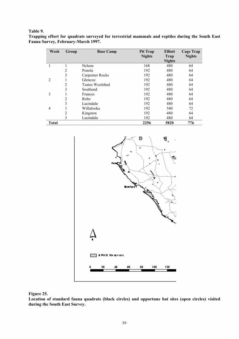
Table 9.Trapping effort for quadrats surveyed for terrestrial mammals and reptiles during the South EastFauna Survey, February-March 1997.

Week Group Base Camp Pit Trap Nights

Elliott Trap

Nights

Cage Trap Nights

1 1 Nelson 168 480 64 2 Penola 192 480 64 3 Carpenter Rocks 192 480 64

2 1 Glencoe 192 480 64 2 Teates Woolshed 192 480 64 3 Southend 192 480 64

3 1 Frances 192 480 64 2 Robe 192 480 64 3 Lucindale 192 480 64

4 1 Willalooka 192 540 72 2 Kingston 192 480 64 3 Lucindale 192 480 64

Total 2256 5820 776

Figure 25.Location of standard fauna quadrats (black circles) and opportune bat sites (open circles) visitedduring the South East Survey.

59

RBRANDLE

Placed Image

RBRANDLE

Note

Accepted set by RBRANDLE

PHOTOGRAPHIC MONITORING POINTS

At each fauna survey quadrat, a permanent

photographic monitoring point was established

according to the South Australian Biological Survey

protocol as described in Owens (2000). These photo

points consist of two steel droppers driven into the

ground, spaced 10 m apart.

Details of the physical environment, vegetation types

and locations of all vegetation survey quadrats are

shown by 1:100,000 map-sheets in Appendix I, with

fauna survey and photo-point quadrats indicated.

DATA MANAGEMENT AND TAXONOMY

Survey data are stored in the Survey database (an

Oracle relational database), accessed via Oracle and

MS Access software. Data were extensively

crosschecked and edited in an MS Excel spreadsheet

prior to importing to PATN.

All taxonomy was thoroughly checked although

taxonomy is regularly updated through the database.

Dubious records were attributed to ‘Genus sp.’ if the

observer or observation was not considered reliable,

and subsequently excluded from the analysis.

FAUNA

A similar system of voucher number usage to that used

for plants enabled later verification or correction of

collected fauna specimens' identifications. Vertebrate

fauna taxonomy is according to Robinson et al. (2000)

and updates by the relevant Museum Curators. No

sub-specific designations were used in the analysis and

reporting as consistent differentiation of certain sub-

species is not possible with a range of observers with

varying skills.

DATA ANALYSIS

The dataset used in the analysis consisted not only of

the data from this survey but fauna data from a number

of other smaller scale surveys conducted in the region

upto 1997 (Table 10). These data were combined to

enable a comprehensive analysis of the fauna

communities present. The fauna quadrat data were

analysed by classification techniques using PATN

exploratory data analysis software (Belbin 1994) to

detect trends and patterns in the data. Vegetation,

mammal, bird and reptile data were separately

extracted from the survey database as listings of

quadrats and species, on which the discussed

taxonomic standardizations were performed. These

data were then formatted into quadrat by species

matrices for input into PATN using a pivot table

generated by MS Excel. Data were analysed using

PATN (Belbin 1994) with a Kulczynski association

measure, then, clustered using unweighted pair-group

arithmetic averaging (UPGMA) with beta (β) set at -

0.1 (Belbin 1994). The final number of groups was

determined by examination of the dendrogram and

two-way table. An indicator value was calculated

using a Yates Correction for continuity (Zar 1984).

Proportional occurrence was also calculated for each

species in each group in Microsoft Excel using the

following formula;

This indicator value was used to determine which

species drove the composition of each group. The

members of each fauna PATN group were also

matched against the floristic type to aid in the

description of habitat preferences or associations with

each fauna assemblage.

Amphibian species were recorded too inconsistently to

warrant any analysis. Similarly, opportunistic data,

being non site-specific, could not be systematically

analysed. These additional data are included in the

discussion of the results.

60

Table 10.

Previous biological surveys conducted in the region whose data contributed the overall analysis of

Date

the fauna of the South East.

Survey Name (Survey No.) No. Quadrats

Bunbury Conservation Reserve (99) December 1997 12

Messent Conservation Park (68) December 1994 12

SE Box and Buloke (84) December 1995 18

Deep Swamp (85) January 1996 12

Gum Lagoon Conservation Park (76) September 1995 and October 1996 29 (mammals and reptiles)

52 (birds)

Tilley Swamp (90) December 1996 16

10*SE Fire Study (64) August, September and October 1994

* bird data not included in analysis

Presence/absence data only were used in the fauna masked out: large snakes and goannas, legless lizards,

analyses, as abundance data were not recorded in a blind snakes, ‘Genus sp.’ records and species with a

systematic manner. frequency of one. Quadrats with only one species after

this mask were also omitted. Thus, the final matrix

Mammals contained 162 quadrats and 28 species.

The initial mammal matrix contained 201 quadrats and

45 species. A number of species were masked out of Birds

the analyses; introduced herbivores, bats, ‘Genus sp.’ The complete bird matrix contained 3168 records; 102

records and species with a frequency of one. Quadrats species and 173 quadrats. Data from the SE Fire Study

with a single species after this mask were retained. (Survey 64) was not available at time of preparation of

The final matrix contained records from 165 quadrats this report. All 'Genus sp.' records were masked out,

and 17 species. as were any species that are very mobile, waterbirds

and night birds. The final matrix contained 61 species

Reptiles and 173 quadrats.

The initial reptile matrix contained 195 quadrats and

59 species (676 records). Several species were

61

Figure 26.Standard survey pit-fall line placed through heathy understorey. Photo: J. Foulkes.

Figure 27.Volunteer checking Elliot trap line in Stringybark woodland survey quadrat. Photo: J. Foulkes.

62

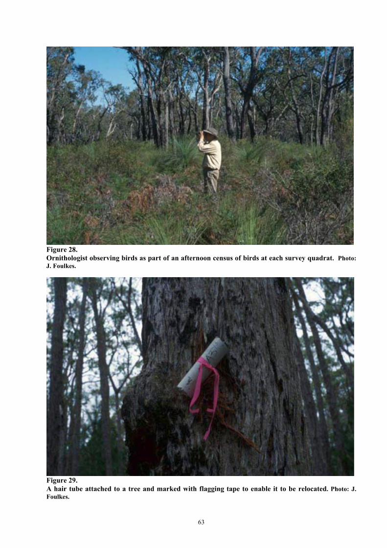
Figure 28.Ornithologist observing birds as part of an afternoon census of birds at each survey quadrat. Photo:J. Foulkes.

Figure 29.A hair tube attached to a tree and marked with flagging tape to enable it to be relocated. Photo: J.Foulkes.

63

a biological survey of the south east south australia

Documents