393-400 promenade des anglais web:...

Spillover Effects of Counter-cyclical Market Regulation: Evidence from the 2008 Ban on Short Sales

March 2010

Institute

EDHEC Risk Institute

393-400 promenade des Anglais06202 Nice Cedex 3Tel.: +33 (0)4 93 18 78 24Fax: +33 (0)4 93 18 78 41E-mail: [email protected]: www.edhec-risk.com

Abraham LiouiProfessor of Finance, EDHEC Business School and Member, EDHEC Risk Institute

2

The ban on shorting had negative effects on the hedge fund industry. It also had a negative impact on the returns and the market quality of the stocks placed off limits by the ban. We look at the impact of the ban on broad market indices in the US and in Europe (the United Kingdom, France, and Germany). Since these indices and their performance are of great concern to the asset management and hedge fund industries, it is important for practitioners and policymakers to understand the impact of changing the rules of the game (banning short sales) on the return distribution of these indices and to assess the potential spillover effects of a counter-cyclical regulation affecting only one segment of the financial market. We show that the ban had a broad impact on the markets. It was responsible for a substantial increase in market volatility. The impact of the ban on the higher moments of index returns is not systematic (skewness and kurtosis of the return distribution of only few indices were affected) or robust (using some robust measures of higher moments makes the impact of the ban disappear). Thus, the ban did not ease the downward pressure in the financial markets. The market seems not to believe that short sellers or the hedge fund industry were responsible for the turmoil of 2008.

The present position paper is a substantial revision of “The Undesirable Effects of Banning Short Sales," an April 2009 position paper from EDHEC Risk Institute.1

In this version, the main changes are as follows: • The sample period has been extended. • Instead of individual stocks, the reaction of the broad indices is compared to the reaction of financial indices. • For each country one short dummy, which corresponds exactly to the length of the short ban period in the country, is used. • For the US, the ban experience of summer 2008 is properly controlled for.• A new measure of liquidity (daily trading volume) has been added as a control variable.

Abstract

1 - A. Lioui. April 2009. “The Undesirable Effects of Banning Short Sales,” EDHEC Risk Institute position paper.

The author wishes to thank Noël Amenc for suggesting this topic. Noël Amenc, René Garcia, Felix Goltz, and Lionel Martellini provided very useful remarks and suggestions on preliminary drafts of this paper. The usual caveats apply. The work presented herein is a detailed summary of academic research conducted by EDHEC Risk Institute. The opinions expressed are these of the author. EDHEC Risk Institute declines all reponsibility for any errors or omissions.

Abraham Lioui is professor of finance at EDHEC Business School. He has published widely in and refereed for leading journals and is regularly invited to the programme committee of the European Finance Association’s annual conference. His research interests in finance revolve around the valuation of financial assets, portfolio management, and risk management. His economics research looks at the relationship between monetary policy and the stock market.

About the Author

3

Table of Contents

4

Introduction ........................................................................................................................................ 5

1. Data and Empirical Method ....................................................................................................... 8

2. Results ........................................................................................................................................... 12

3. Concluding Remarks ................................................................................................................... 22

References ......................................................................................................................................... 15

EDHEC Risk Institute Position Papers and Publications (2007-2010) .................................. 16

5

On 18 September 2008 the SEC surprised the US financial markets by issuing an emergency order prohibiting the short selling of about 1,000 stocks of financial institutions from the NYSE, the AMEX, and the NASDAQ. Market authorities in the UK, France, Germany, and elsewhere took similar steps. The preamble to the SEC press release stated:

“The Securities and Exchange Commission, acting in concert with the UK Financial Services Authority, took temporary emergency action to prohibit short selling in financial companies to protect the integrity and quality of the securities market and strengthen investor confidence”.

The press release also attempts to justify the move:

“Under normal market conditions, short selling contributes to price efficiency and adds liquidity to the markets. At present, it appears that unbridled short selling is contributing to the recent, sudden price declines in the securities of financial institutions unrelated to true price valuation”.

The SEC, in short, is blaming short sellers for the sharp drop in the prices of financial stocks. It suggests that these drops have little to do with fundamentals. It is no secret that the hedge fund industry was the target of this measure. And the industry—long/short equity, convertible arbitrage, and relative value managers—did indeed suffer from this disruption of its activity.

This episode comes after a period of great deregulation of short selling. By 6 July 2007 the SEC had removed some of the major obstacles, the uptick rule in particular, that had once stood in the way

of short selling. This decision was made after a transition period, starting in May 2005, during which the uptick rule was removed only for a pilot group of stocks. Diether, Lee, and Werner (2009) showed explicitly that the removal of this rule did not affect the daily returns of these stocks. Boehmer, Jones, and Zhang (2008) showed that the repeal of the uptick rule neither destabilised prices nor contributed to the great increase in volatility of the summer of 2007. These conclusions dovetail with the SEC statement that short sellers contributed to market efficiency “under normal conditions”.

Recent empirical evidence2 suggests that, on the whole, the ban had a negative impact on the returns and market quality of the off-limits stocks. In this paper, our purpose is to assess the broader impact (spillover effects) on the markets of this counter-cyclical regulation. We thus look at the impact of the ban on market indices in the US and in European markets (the United Kingdom, France, and Germany) where short selling was banned. Since these indices are the underlying assets of extremely active derivatives markets (options and futures among others), it is important for both practitioners and policymakers to understand the impact of changing the rules (banning short sales) on the return distribution of these indices.

Before we summarise our empirical findings, it is useful to set up the potential effects of such regulatory action. Most of the academic literature on short selling focuses on the impact of short sale constraints on the stocks subject to these constraints. Miller’s (1977) seminal work predicts that, under symmetric information, short sale constraints will cause over-pricing, reduce volatility, and make skewness less negative.

Introduction

2 - See Autore, Billingsley, and Kovacs (2009) and the references therein.

6

These effects are a direct consequence of keeping the pessimistic traders out ofthe market. Diamond and Verrecchia (1987) have shown that, under rational expectations, Miller’s mechanism may not be at play. Rational investors will integrate into the prices the fact that traders with negative information are being kept out of the market. Recently, Bai, Chang, and Wang (2006) even showed that, under asymmetric information, prices may fall, volatility may increase, and return skewness may worsen. After all, prices become less informative when short sellers are kept out of the market and there will thus be less demand for the constrained assets.

Empirical evidence lends credence to the notion that restrictions on short sales will cause the stocks subject to these restrictions to suffer excessive volatility, more negative skewness, and higher kurtosis. The market quality of the stocks placed off limits deteriorates, volatility increases, and, at best, return skewness is not affected by the measure. Short sellers are thus clearly considered informed sophisticated traders.3

It seems that there are no studies that address the effects of limits on short sales that may spill over to all segments of the market. Bai, Chang, and Wang (2006), for example, develop their theory in a market where one risk-free asset (not constrained) and one risky asset (constrained) are traded. All the same, the impact of the ban on standard market indicators can be looked into and fundamental questions can be answered. Did the ban increase the overall dispersion of investor opinions? The diagnostic could be done by looking at the impact of the ban on the volatility of the indices. Did the ban curb the general market pessimism prevailing around the ban announcement?

Looking at the impact of the ban on the skewness of index returns could tell us. Finally, for the off-limits stocks, there may be configurations in which these limitations lead to a market crash.

Hong and Stein (2003) and Bai, Chang, and Wang (2006) show that, when the uncertainty as perceived by uninformed investors increases, there may be a sudden discrete drop in the prices and a subsequent huge increase in volatility. So it would be interesting to assess the impact of the ban on the tailbehaviour (kurtosis) of the returns of these indices.

Our empirical findings can be summarised as follows. The ban has had a considerable impact on the daily volatility of the indices. This impact is the symptom of an increase in the dispersion of investors’ beliefs about future prices. There is no evidence that this ban affected other features of the return distribution of the indices. In particular, if the markets were under downward pressure, the ban did not manage to ease it.

A reasonable conclusion is that short sellers are key figures in the financial markets. Moreover, market participants do not seem to believe that there was any particular condition that justified the measure taken by the SEC and others. Last, the hedge fund industry is certainly not to be blamed for trying to make money by exploiting the overvaluation of badly managed financial institutions. The rest of the paper is organised as follows. In the next section we describe our data and our empirical method. We then describe the results. In the final section we reflect on the possible lessons to be learned from this regulatory episode and discuss the potential risks of the

Introduction

3 - Ample empirical evidence confirms this. See, for example, Purnanandam and Seyhun (2009).

7

Introduction

recent (February 2010) regulatory move of the SEC and the EU market regulatory authority.

8

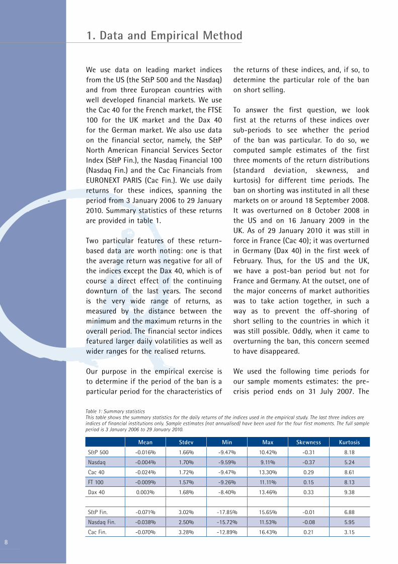
We use data on leading market indices from the US (the S&P 500 and the Nasdaq) and from three European countries with well developed financial markets. We use the Cac 40 for the French market, the FTSE 100 for the UK market and the Dax 40 for the German market. We also use data on the financial sector, namely, the S&P North American Financial Services Sector Index (S&P Fin.), the Nasdaq Financial 100 (Nasdaq Fin.) and the Cac Financials from EURONEXT PARIS (Cac Fin.). We use daily returns for these indices, spanning the period from 3 January 2006 to 29 January 2010. Summary statistics of these returns are provided in table 1.

Two particular features of these return-based data are worth noting: one is that the average return was negative for all of the indices except the Dax 40, which is of course a direct effect of the continuing downturn of the last years. The second is the very wide range of returns, as measured by the distance between the minimum and the maximum returns in the overall period. The financial sector indices featured larger daily volatilities as well as wider ranges for the realised returns.

Our purpose in the empirical exercise is to determine if the period of the ban is a particular period for the characteristics of

the returns of these indices, and, if so, to determine the particular role of the ban on short selling.

To answer the first question, we look first at the returns of these indices over sub-periods to see whether the period of the ban was particular. To do so, we computed sample estimates of the first three moments of the return distributions (standard deviation, skewness, and kurtosis) for different time periods. The ban on shorting was instituted in all these markets on or around 18 September 2008. It was overturned on 8 October 2008 in the US and on 16 January 2009 in the UK. As of 29 January 2010 it was still in force in France (Cac 40); it was overturned in Germany (Dax 40) in the first week of February. Thus, for the US and the UK, we have a post-ban period but not for France and Germany. At the outset, one of the major concerns of market authorities was to take action together, in such a way as to prevent the off-shoring of short selling to the countries in which it was still possible. Oddly, when it came to overturning the ban, this concern seemed to have disappeared.

We used the following time periods for our sample moments estimates: the pre-crisis period ends on 31 July 2007. The

1. Data and Empirical Method

Mean Stdev Min Max Skewness Kurtosis

S&P 500 -0.016% 1.66% -9.47% 10.42% -0.31 8.18

Nasdaq -0.004% 1.70% -9.59% 9.11% -0.37 5.24

Cac 40 -0.024% 1.72% -9.47% 13.30% 0.29 8.61

FT 100 -0.009% 1.57% -9.26% 11.11% 0.15 8.13

Dax 40 0.003% 1.68% -8.40% 13.46% 0.33 9.38

S&P Fin. -0.071% 3.02% -17.85% 15.65% -0.01 6.88

Nasdaq Fin. -0.038% 2.50% -15.72% 11.53% -0.08 5.95

Cac Fin. -0.070% 3.28% -12.89% 16.43% 0.21 3.15

Table 1: Summary statisticsThis table shows the summary statistics for the daily returns of the indices used in the empirical study. The last three indices are indices of financial institutions only. Sample estimates (not annualised) have been used for the four first moments. The full sample period is 3 January 2006 to 29 January 2010.

9


crisis period up to the ban on short selling ends on 17 September 2008. The ban period ends on 8 October 2008 for the US and, for the UK, on 16 January 2009. For the US and the UK, the post-ban period ends on 29 January 2010, the end of our sample period. Outliers are likely to be in the last two years of our sample and therefore using an extended sample for the ban period limits their impact.

Marsh and Niemer (2008) and Lioui (2009) have also compared sample estimates of moments of the returns of the off-limits stocks. However, as noted by Lioui (2009), the sample estimates are very sensitive to the outliers and this problem may be compounded by the short duration of the ban period. As a consequence, we also computed robust estimates of the skewness and the kurtosis of the returns on the indices. But rather than using a particular method to eliminate outliers, we use measures based on quintiles obtained from the empirical distribution, as advocated by Kim and White (2004). The robust measures are thus less subject to the arbitrariness of outlier identification.

The robust measure of skewness we use is:

Robust skewness =

Q3 +Q1 − 2Q2

Q3 −Q1 (1)

where Qi is the ith quartile of the return distribution, Q1 = F −1 0.25( ) , Q2 = F −1 0.5( ) and

Q3 = F −1 0.75( ) , where F is the cumulative distribution. This measure, known as the Bowley (1920) measure, is equal to 0 for a symmetric distribution. The denominator re-scales the coefficient so that the maximum value for this measure is 1, representing extreme right skewness, and the minimum value is –1, representing extreme left skewness.

The robust measure of kurtosis we use is:

Robust kurtosis =

F −1 0.975( ) − F −1 0.025( )F −1 0.75( ) − F −1 0.25( )

− 2.91 (2)

where F is the cumulative distribution function. This measure was first suggested by Crow and Siddiqui (1967) and it takes on the value of 2.91 for standard normal distribution. The two robust measures here have the desirable properties mentioned by Kim and White (2004).

In a second step, we attempt to determine whether the crisis or the ban or both were responsible for the events during the period of the ban. For each index, we built a time series of the three first moments: standard deviation, skewness and kurtosis. Daily volatility is obtained by using a rolling window of the sixty previous days: for each day, we calculated the standard deviation of the returns of the previous sixty days. We did the same for the skewness and the kurtosis. Since two successive observations have fifty-nine overlapping observations, the time series obtained are highly persistent. It is thus natural to use an AR(1) process as a baseline data-generating process. This AR(1) formulation is augmented by other variables that we describe hereafter.

We want to disentangle the effects of the ban from those of other events that took place over the same period. To distinguish between the effects of the financial crisis, which began in the summer of 2007, and those of the ban, which began in September 2008, we built several dummy variables. Crisis7 is a crisis dummy (equal to 0 from 3 January 2006 to 31 July 2007, and to 1 until 29 January 2010). For the S&P 500, the Nasdaq, the S&P Fin. and the Nasdaq Fin., the short dummies are defined as follows: the first short dummy (short1) is equal to 0 from 3 January 2006 to 14 July 2008, and from 16 August 2008 to 29 January 2010; it is equal to 1 from 15 July 2008 to 15 August 2008. The second dummy (short2) is equal to 0 from 3 January 2006 to 17 September 2008 and from 9 October 2008 to 31 January 2010;

10

it is equal to 1 from 18 September 2008 to 8 October 2008. For the CAC, Dax, FT 100 and Cac Fin., the first short dummy (short1) is equal to 0 from 3 January 2006 to 17 September 2008 and from 9 October 2008 to 29 January 2010; it is equal to 1 from 18 September 2008 to 8 October 2008. The second dummy is defined as follows: for the Cac, Cac Fin., and the Dax, it is equal to 0 from 3 January 2006 to 17 September 2008; it is equal to 1 from 18 September 2008 to 29 January 2010. For the FTSE 100, short2 is equal to 0 from 3 January 2006 to 17 September 2008; it is equal to 1 from 18 September 2008 to 16 January 2009; it is equal to 0 again from 17 January 2009 to 29 January 2010.

For each country/index we thus have a dummy that covers the exact ban period starting on 18 September 2008. We also have an additional short dummy whose intent is as follows. For the US, and thus the S&P 500, the Nasdaq, and the corresponding financial sector indices, we have a dummy that covers the short ban experience following the emergency order of 15 July 2008. Since the two short ban episodes were close, it seemed to us useful to isolate the impact of the first short ban period from that of the second. For France (Cac 40) and Germany (Dax 40), the ban was still in place at the end of the sample period. Nevertheless, it turns out that, for market volatility at least (as shown below), the pattern of the moments of these two indices was similar to that of the US indices. One observes an inverse U shape from September 2008 to the end of the sample. When a dummy that covers only the ban period for France, for example, is taken, the impact of the ban would be negligible ex post as a result of the inverse U shape. As a consequence, it is likely that if the ban were responsible for any change in volatility, it would have been in the days

just after the SEC banned short sales. We therefore added a second dummy for France and Germany. Rather than choosing an arbitrary period, the second short dummy for the Cac 40 and the Dax 40 corresponds simply to the ban period in the US. Finally, the UK provides a hybrid case, since the ban was overturned but later than in the US. For comparison purposes, we also used a second dummy for the UK, which corresponds to the ban period in the US.

In addition to the dummy variables, we added several control variables that attempt to capture current market conditions. First, for each index moment (standard deviation, skewness, and kurtosis), we added the corresponding market return. We also added the log of the trading volume as a measure of local market liquidity. Such data were not available for the Dax 40 and the financial sector indices, so they were not introduced. To capture counterparty risk we used the credit spread defined, in keeping with the literature, as the spread on a BAA and an AAA corporate bond yields. It is the usual proxy for the default risk premium. Since this variable is extremely persistent, we used the innovation in this spread (the first difference) as a measure of the changes in market default risk premium (cs in the tables). The TED spread is the interest rate difference between the prime rate and the T-bill rate. Since it is extremely persistent, we also used the innovation in this spread (first difference) as a measure of the changes in market liquidity (ted in the tables). As Brunnermeier (2009) notes, it is a good measure of the changes in (money) market liquidity.


11


For each index i, we thus run the following regression:

where momi ,t is the sample or, whenever

relevant, the robust estimate of the moment, and crisis7, short1, and short2 are the dummies related to the crisis and the short sale ban periods as described above. cs and ted are the innovation in the credit spread and the TED spread respectively.

In the following section we present the results.

momi ,t = α i ,0 + α i ,1 × momi ,t −1 + α i ,2 × index i ,t + α i ,3 × ln(volumei ,t )

+α i ,4 × cs i ,t + α i ,5 × tedi ,t + α i ,6 × crisis 7i ,t

+α i ,7 × short1i ,t + α i ,8 × short 2i ,t + ε i ,t

12

2. Results

As noted in the introduction, the aim of the ban on short selling was to stop the fall in the prices of the stocks of financial companies. The repercussions of this measure on the stock markets are analysed by looking, successively, at the impact on the daily volatility, skewness, and kurtosis of the index returns.

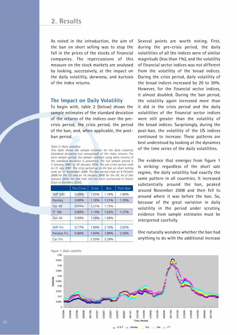
The Impact on Daily VolatilityTo begin with, table 2 (below) shows the sample estimates of the standard deviation of the returns of the indices over the pre-crisis period, the crisis period, the period of the ban, and, when applicable, the post-ban period.

Table 2: Daily volatilityThis table shows the sample estimate for the daily volatility (standard deviation not annualised) of the index returns. For each sample period, the sample estimate using daily returns of the standard deviation is presented. The full sample period is 3 January 2006 to 29 January 2010. The pre-crisis period ends on 31 July 2007. The crisis period up to the ban on short selling ends on 17 September 2008. The ban period ends on 8 October 2008 for the US and on 16 January 2009 for the UK. As of late January 2010, the ban had still not been overturned in France (Cac) or Germany (Dax).

Pre-Crisis Crisis Ban Post-Ban

S&P 500 0.69% 1.05% 1.18% 1.66%

Nasdaq 0.88% 1.18% 1.31% 1.70%

Cac 40 0.94% 1.21% 1.72%

FT 100 0.80% 1.14% 1.62% 1.57%

Dax 40 0.99% 1.16% 1.68%

S&P Fin. 0.77% 1.80% 2.10% 3.02%

Nasdaq Fin. 0.86% 1.64% 1.88% 2.50%

Cac Fin. 2.55% 3.28%

Several points are worth noting. First, during the pre-crisis period, the daily volatilities of all the indices were of similar magnitude (less than 1%), and the volatility of financial sector indices was not different from the volatility of the broad indices. During the crisis period, daily volatility of the broad indices increased by 20 to 30%. However, for the financial sector indices, it almost doubled. During the ban period, the volatility again increased more than it did in the crisis period and the daily volatilities of the financial sector indices were still greater than the volatility of the broad indices. Surprisingly, during the post-ban, the volatility of the US indices continued to increase. These patterns are best understood by looking at the dynamics of the time series of the daily volatilities.

The evidence that emerges from figure 1is striking: regardless of the short sale regime, the daily volatility had exactly the same pattern in all countries. It increased substantially around the ban, peaked around November 2008 and then fell to around where it was before the ban. So, because of the great variation in daily volatility in the period under scrutiny, evidence from sample estimates must be interpreted carefully.

One naturally wonders whether the ban had anything to do with the additional increase

Figure 1: Daily volatility

in daily volatility in the period of the ban, which was also a period of ongoing financial crisis. The regression approach, as it happens, is meant to disentangle the two effects. We used the time series of daily volatility as the explained variable, and several explanatory variables as in equation (1). The results are shown in table 3.

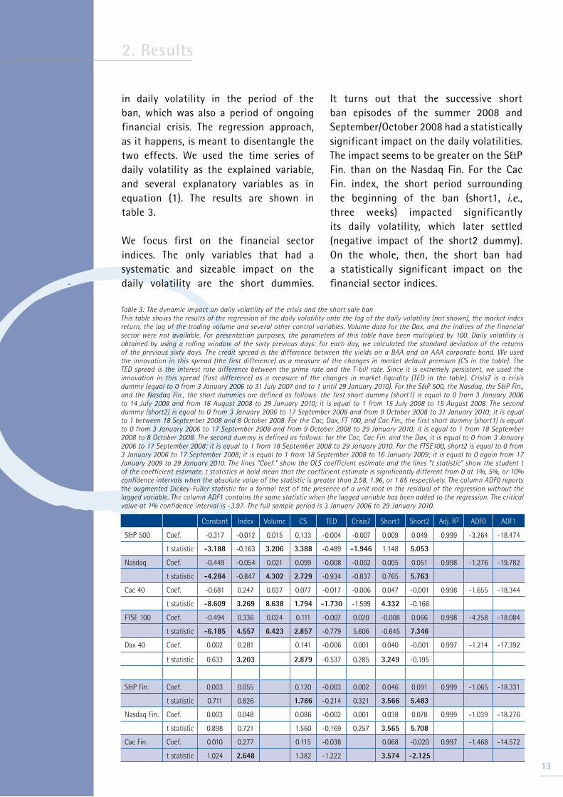
We focus first on the financial sector indices. The only variables that had a systematic and sizeable impact on the daily volatility are the short dummies.

It turns out that the successive short ban episodes of the summer 2008 and September/October 2008 had a statistically significant impact on the daily volatilities. The impact seems to be greater on the S&P Fin. than on the Nasdaq Fin. For the Cac Fin. index, the short period surrounding the beginning of the ban (short1, i.e., three weeks) impacted significantly its daily volatility, which later settled (negative impact of the short2 dummy). On the whole, then, the short ban had a statistically significant impact on the financial sector indices.

2. Results

13

Table 3: The dynamic impact on daily volatility of the crisis and the short sale banThis table shows the results of the regression of the daily volatility onto the lag of the daily volatility (not shown), the market index return, the log of the trading volume and several other control variables. Volume data for the Dax, and the indices of the financial sector were not available. For presentation purposes, the parameters of this table have been multiplied by 100. Daily volatility is obtained by using a rolling window of the sixty previous days: for each day, we calculated the standard deviation of the returns of the previous sixty days. The credit spread is the difference between the yields on a BAA and an AAA corporate bond. We used the innovation in this spread (the first difference) as a measure of the changes in market default premium (CS in the table). The TED spread is the interest rate difference between the prime rate and the T-bill rate. Since it is extremely persistent, we used the innovation in this spread (first difference) as a measure of the changes in market liquidity (TED in the table). Crisis7 is a crisis dummy (equal to 0 from 3 January 2006 to 31 July 2007 and to 1 until 29 January 2010). For the S&P 500, the Nasdaq, the S&P Fin.,and the Nasdaq Fin., the short dummies are defined as follows: the first short dummy (short1) is equal to 0 from 3 January 2006 to 14 July 2008 and from 16 August 2008 to 29 January 2010; it is equal to 1 from 15 July 2008 to 15 August 2008. The second dummy (short2) is equal to 0 from 3 January 2006 to 17 September 2008 and from 9 October 2008 to 31 January 2010; it is equal to 1 between 18 September 2008 and 8 October 2008. For the Cac, Dax, FT 100, and Cac Fin., the first short dummy (short1) is equal to 0 from 3 January 2006 to 17 September 2008 and from 9 October 2008 to 29 January 2010; it is equal to 1 from 18 September 2008 to 8 October 2008. The second dummy is defined as follows: for the Cac, Cac Fin. and the Dax, it is equal to 0 from 3 January 2006 to 17 September 2008; it is equal to 1 from 18 September 2008 to 29 January 2010. For the FTSE100, short2 is equal to 0 from 3 January 2006 to 17 September 2008; it is equal to 1 from 18 September 2008 to 16 January 2009; it is equal to 0 again from 17 January 2009 to 29 January 2010. The lines “Coef.” show the OLS coefficient estimate and the lines “t statistic” show the student t of the coefficient estimate. t statistics in bold mean that the coefficient estimate is significantly different from 0 at 1%, 5%, or 10% confidence intervals when the absolute value of the statistic is greater than 2.58, 1.96, or 1.65 respectively. The column ADF0 reports the augmented Dickey-Fuller statistic for a formal test of the presence of a unit root in the residual of the regression without the lagged variable. The column ADF1 contains the same statistic when the lagged variable has been added to the regression. The critical value at 1% confidence interval is -3.97. The full sample period is 3 January 2006 to 29 January 2010.

Constant Index Volume CS TED Crisis7 Short1 Short2 Adj. R2 ADF0 ADF1

S&P 500 Coef. -0.317 -0.012 0.015 0.133 -0.004 -0.007 0.009 0.049 0.999 -3.264 -18.474

t statistic -3.188 -0.163 3.206 3.388 -0.489 -1.946 1.148 5.053

Nasdaq Coef. -0.449 -0.054 0.021 0.099 -0.008 -0.002 0.005 0.051 0.998 -1.276 -19.782

t statistic -4.284 -0.847 4.302 2.729 -0.934 -0.837 0.765 5.763

Cac 40 Coef. -0.681 0.247 0.037 0.077 -0.017 -0.006 0.047 -0.001 0.998 -1.655 -18.344

t statistic -8.609 3.269 8.638 1.794 -1.730 -1.599 4.332 -0.166

FTSE 100 Coef. -0.494 0.336 0.024 0.111 -0.007 0.020 -0.008 0.066 0.998 -4.258 -18.084

t statistic -6.185 4.557 6.423 2.857 -0.779 5.606 -0.645 7.346

Dax 40 Coef. 0.002 0.281 0.141 -0.006 0.001 0.040 -0.001 0.997 -1.214 -17.392

t statistic 0.633 3.203 2.879 -0.537 0.285 3.249 -0.195

S&P Fin. Coef. 0.003 0.055 0.120 -0.003 0.002 0.046 0.091 0.999 -1.065 -18.331

t statistic 0.711 0.826 1.786 -0.214 0.321 3.566 5.483

Nasdaq Fin. Coef. 0.003 0.048 0.086 -0.002 0.001 0.038 0.078 0.999 -1.039 -18.276

t statistic 0.898 0.721 1.560 -0.169 0.257 3.565 5.708

Cac Fin. Coef. 0.010 0.277 0.115 -0.038 0.068 -0.020 0.997 -1.468 -14.572

t statistic 1.024 2.648 1.382 -1.222 3.574 -2.125

14

Looking now at the broad indices, the results seem somewhat different. First, it seems that the September ban on short selling had the greatest impact on the volatility of the US markets; the impact of the summer 2008 episode, marginal, was not statistically significant. Although the regressions do not contain the same variables for every index, it is worth noting that the impact of the ban on these broad indices was roughly half of the impact on the financial sector indices. Similarly, for the UK, the ban had a substantial and statistically significant impact on the volatility of the FTSE 100. That the ban period was slightly longer in the UK than in the US does not seem to be relevant (short1 for the UK is not significant). Finally, for the Cac 40 and the Dax 40, the impact of the September ban was immediate and the fact that the ban was still in place more than one year later made no difference to its impact.

As table 3 also shows, two other variables, innovation in the credit spread and trading volume, seem to have had a positive impact on the daily volatility. This result is comforting since these two variables were intended to capture the impact of two major phenomena present over the period of the ban: the lack of confidence following the Lehman Brothers bankruptcy (credit spread) and the liquidity shortage (trading volume). Since the short dummies survive the presence of these two variables, these dummies do in fact capture the marginal impact of the regulatory action on the daily volatilities. The impact of the TED is negative, meaning that daily volatility decreases when TED innovation is positive. After all, an increase in the TED means a reduction in market-wide liquidity. As less capital is available for trading on financial markets, the market fluctuates less wildly. The impact of the innovation in TED, as it happens,

was systematically negative although not always significant.

In sum, the empirical evidence supports the view that the effects of the ban appeared not only in the financial sector but also in the broader markets. What perspective does this evidence provide on the existing theories of short selling and market equilibrium? The reaction of the financial sector indices is consistent with a theory accounting explicitly for asymmetric information. In this case, uninformed investors will generally reduce demand for stocks placed off limits to short sellers, a reduction that will, in turn, reduce the prices and increase the volatility of these stocks. The reaction of the broad indices may also reflect a growing lack of confidence of the uninformed or less sophisticated investors following the measures taken by the market authorities. The markets clearly view the real world as a world of asymmetric information and, as such, the market authorities must be aware that regulatory actions do not have a unique equilibrium implication.

Another explicit motivation for the ban was to ease the downward pressure on the financial stocks targeted by short sellers. Pessimism prevailed at the time; it is worth looking at the impact of the ban on these prevailing views. We address this issue below; that is, we attempt to determine whether the ban had an impact on the skewness of the index returns.

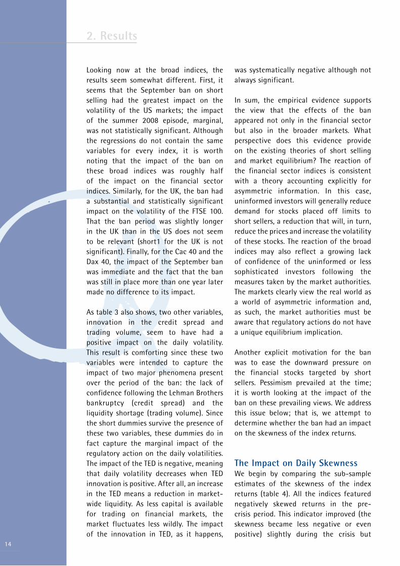
The Impact on Daily SkewnessWe begin by comparing the sub-sample estimates of the skewness of the index returns (table 4). All the indices featured negatively skewed returns in the pre-crisis period. This indicator improved (the skewness became less negative or even positive) slightly during the crisis but

2. Results

worsened again for the US during the ban, while it pursued its improvement for the European indices. There is no particular difference between the broad indices and the financial sector indices. As a consequence, sample estimates of skewness make it hard to draw a conclusion about the impact of the ban on the skewness. The evidence from robust measures of skewness is not consistent with these findings. In table 5 we show the robust measure of skewness.

Table 5: Robust daily skewnessThis table shows a robust estimation for the daily skewness for the index returns. We use the robust measure of skewness introduced in Kim and White (2004), who define it as follows:

SK =

Q3 +Q1 − 2Q2

Q3 −Q1

where Qi is the ith quartile of the return distribution,

Q1 = F −1 0.25( ) , Q2 = F −1 0.5( ) and Q3 = F −1 0.75( ), where F is the cumulative distribution. The pre-crisis period ends on 31 July 2007. The crisis period up to the ban on short selling ends on 17 September 2008. The ban period ends on 8 October 2008 for the US and on 16 January 2009 for the UK. As of late January 2010, the ban had still not been overturned in France (Cac) or Germany (Dax). The full sample period is 3 January 2006 to 29 January 2010.

Crisis Pre-Crisis Ban Post-Ban

S&P 500 -0.15 -0.09 -0.10 -0.10

Nasdaq -0.13 -0.12 -0.12 -0.07

Cac 40 0.03 0.00 -0.03

FTSE 100 0.08 0.03 0.00 0.01

Dax 40 -0.04 -0.14 -0.11

S&P Fin. -0.06 -0.08 -0.08 -0.07

Nasdaq Fin. -0.11 -0.06 -0.07 -0.08

Cac Fin. 0.18 0.02

2. Results

15

Table 4: Daily skewnessThis table shows the sample estimates for the daily skewness of the index returns. For each sample period, the sample estimate (the third central moment divided by the cube of the standard deviation) using daily returns is presented in the table on the left. The table shows the statistic used to test whether the obtained value of skewness is significantly different from 0. The statistic is

T × sample estimate , which is distributed as an N(0,6) under normality (Bai and Ng 2005). The pre-crisis period ends on 31 July 2007. The crisis period up to the ban on short selling ends on 17 September 2008. The ban period ends on 8 October 2008 for the US and on 16 January 2009 for the UK. As of late January 2010, the ban had still not been overturned in France (Cac) or Germany (Dax). The critical value for the test at 5% confidence is 1.96. The full sample period is 3 January 2006 to 29 January 2010.

Pre-Crisis Crisis Ban Post-Ban Pre-Crisis Crisis Ban Post-Ban

S&P 500 -0.58 -0.40 -1.05 -0.31 S&P 500 -4.68 -4.22 -11.27 -4.06

Nasdaq -0.29 -0.17 -0.80 -0.37 Nasdaq -2.37 -1.83 -8.66 -4.79

Cac 40 -0.46 -0.21 0.29 Cac 40 -3.65 -2.24 3.78

FTSE 100 -0.51 -0.10 0.22 0.15 FTSE 100 -4.09 -1.11 2.49 2.00

Dax 40 -0.43 -0.59 0.33 Dax 40 -3.44 -6.23 4.24

S&P Fin. -0.56 0.13 -0.26 -0.01 S&P Fin. -4.44 1.34 -2.71 -0.15

Nasdaq Fin. -0.21 0.47 -0.06 -0.08 Nasdaq Fin. -1.66 4.95 -0.67 -1.06

Cac Fin. 0.44 0.21 Cac Fin. 2.16 1.91

16

The skewness of returns of the US indices improved during the crisis/ban periods, whereas it worsened for European indices. These contradictory results make it clear how careful one should be when comparing sample or even robust estimates for

different sampling periods. A glance at the time series of this indicator explains why sample or robust estimates have no hope of reliably capturing the impact of the ban.

2. Results

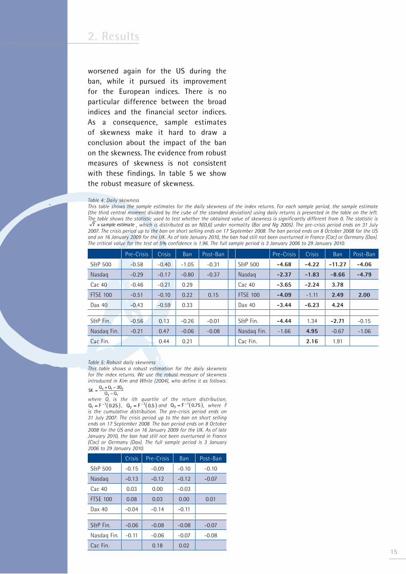
Table 6: The dynamic impact on daily skewness of the crisis and the short sale banThis table shows the results of the regression of the daily skewness onto the lag of the daily skewness (not presented), the market index return, the log of the trading volume and several other control variables. Daily skewness is obtained by using a rolling window of the sixty previous days: for each day, we calculated the skewness of the returns of the previous sixty days. The legend for table 3 applies here.


S&P 500 Coef. 0.303 1.157 -0.014 -0.217 -0.042 0.015 0.018 0.001 0.953 -3.650 -21.418

t statistic 0.963 4.841 -0.994 -1.648 -1.381 1.235 0.689 0.020

Nasdaq Coef. 0.139 0.501 -0.007 -0.197 -0.034 0.006 0.000 -0.026 0.963 -3.335 -22.258

t statistic 0.491 2.899 -0.515 -2.021 -1.508 0.890 -0.001 -1.067

Cac 40 Coef. -0.157 1.751 0.008 -0.076 -0.003 0.019 0.038 0.004 0.927 -4.899 -22.245

t statistic -0.788 9.159 0.704 -0.699 -0.113 2.008 1.350 0.512

FTSE 100 Coef. -0.176 1.720 0.007 -0.307 -0.026 0.019 0.037 0.030 0.924 -4.565 -21.594

t statistic -0.766 8.122 0.690 -2.771 -1.029 2.402 1.226 2.180

Dax 40 Coef. -0.034 2.600 0.173 0.057 0.015 -0.037 0.035 0.894 -5.923 -24.423

t statistic -3.579 9.450 1.124 1.650 1.233 -0.974 2.682

S&P Fin. Coef. -0.011 0.548 -0.078 -0.005 0.017 0.048 -0.017 0.956 -3.622 -21.426

t statistic -1.571 4.408 -0.625 -0.171 1.947 1.942 -0.570

Nasdaq Fin. Coef. -0.006 0.554 -0.116 0.022 0.011 0.046 -0.037 0.967 -3.252 -22.698

t statistic -1.159 4.673 -1.186 0.975 1.610 2.309 -1.540

Cac Fin. Coef. 0.029 0.394 -0.056 -0.141 0.094 -0.029 0.950 -3.506 -13.575

t statistic 2.200 2.936 -0.521 -3.517 3.282 -2.142

Figure 2: Daily skewness

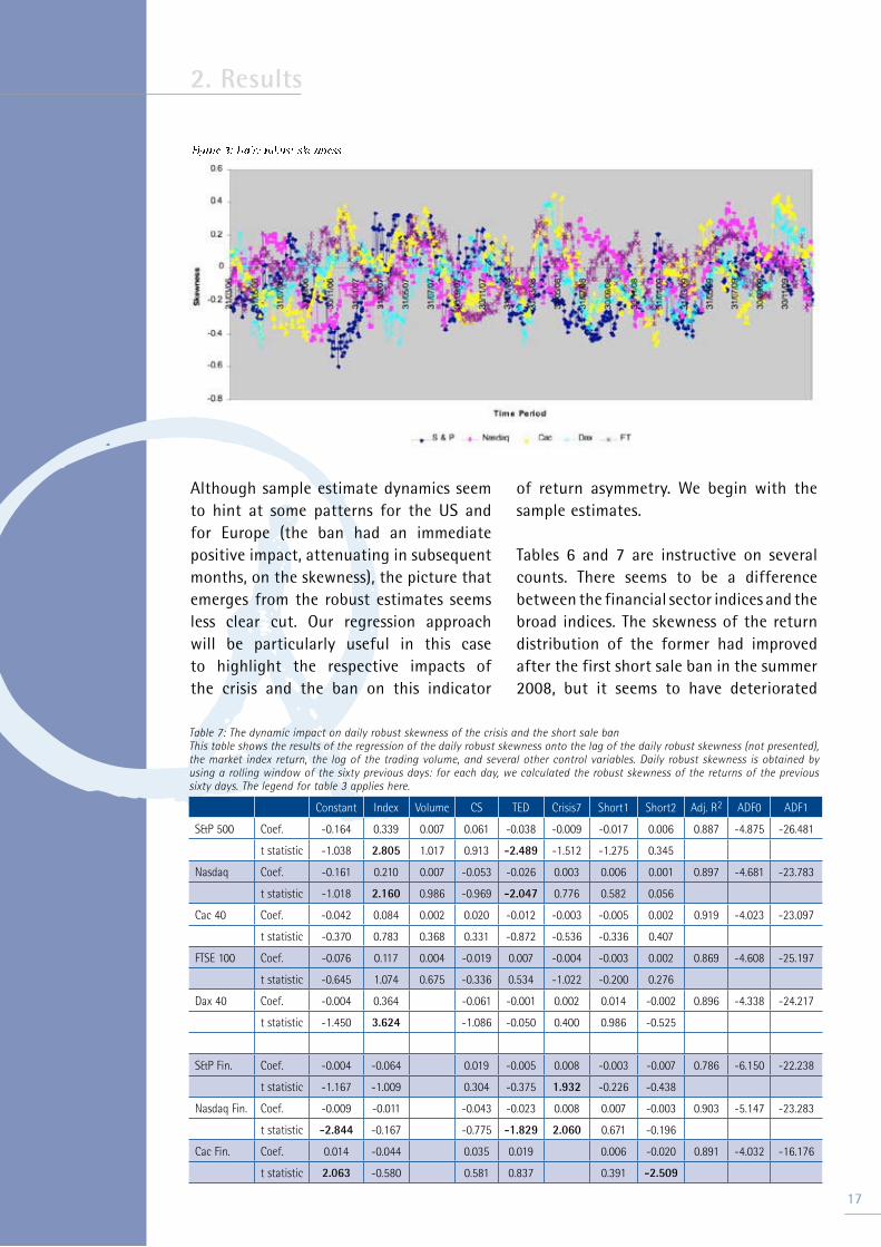
Although sample estimate dynamics seem to hint at some patterns for the US and for Europe (the ban had an immediate positive impact, attenuating in subsequent months, on the skewness), the picture that emerges from the robust estimates seems less clear cut. Our regression approach will be particularly useful in this case to highlight the respective impacts of the crisis and the ban on this indicator

of return asymmetry. We begin with the sample estimates.

Tables 6 and 7 are instructive on several counts. There seems to be a difference between the financial sector indices and the broad indices. The skewness of the return distribution of the former had improved after the first short sale ban in the summer 2008, but it seems to have deteriorated

2. Results

17

Figure 3: Daily robust skewness

Table 7: The dynamic impact on daily robust skewness of the crisis and the short sale banThis table shows the results of the regression of the daily robust skewness onto the lag of the daily robust skewness (not presented), the market index return, the log of the trading volume, and several other control variables. Daily robust skewness is obtained by using a rolling window of the sixty previous days: for each day, we calculated the robust skewness of the returns of the previous sixty days. The legend for table 3 applies here.


S&P 500 Coef. -0.164 0.339 0.007 0.061 -0.038 -0.009 -0.017 0.006 0.887 -4.875 -26.481

t statistic -1.038 2.805 1.017 0.913 -2.489 -1.512 -1.275 0.345

Nasdaq Coef. -0.161 0.210 0.007 -0.053 -0.026 0.003 0.006 0.001 0.897 -4.681 -23.783

t statistic -1.018 2.160 0.986 -0.969 -2.047 0.776 0.582 0.056

Cac 40 Coef. -0.042 0.084 0.002 0.020 -0.012 -0.003 -0.005 0.002 0.919 -4.023 -23.097

t statistic -0.370 0.783 0.368 0.331 -0.872 -0.536 -0.336 0.407

FTSE 100 Coef. -0.076 0.117 0.004 -0.019 0.007 -0.004 -0.003 0.002 0.869 -4.608 -25.197

t statistic -0.645 1.074 0.675 -0.336 0.534 -1.022 -0.200 0.276

Dax 40 Coef. -0.004 0.364 -0.061 -0.001 0.002 0.014 -0.002 0.896 -4.338 -24.217

t statistic -1.450 3.624 -1.086 -0.050 0.400 0.986 -0.525

S&P Fin. Coef. -0.004 -0.064 0.019 -0.005 0.008 -0.003 -0.007 0.786 -6.150 -22.238

t statistic -1.167 -1.009 0.304 -0.375 1.932 -0.226 -0.438

Nasdaq Fin. Coef. -0.009 -0.011 -0.043 -0.023 0.008 0.007 -0.003 0.903 -5.147 -23.283

t statistic -2.844 -0.167 -0.775 -1.829 2.060 0.671 -0.196

Cac Fin. Coef. 0.014 -0.044 0.035 0.019 0.006 -0.020 0.891 -4.032 -16.176

t statistic 2.063 -0.580 0.581 0.837 0.391 -2.509

18

during the second short sale ban period. The deterioration is not statistically significant. For the broad indices (S&P 500 and Nasdaq), the ban seems to have no impact on the skewness of their returns. Some improvement occurred for the skewness of the FTSE 100. The September 2008 episode had no impact on the skewness of the returns of six of the eight indices.

The ban has no statistically significant impact on the skewness of the index returns. No other variable seems to have any systematic impact on the skewness dynamics. At this point, then, it would be fair to conclude that the ban had no significant impact on the skewness of the indices. The analysis above offers two lessons. First, the standard approach to analysing the impact of the ban is to compare sample estimates over different periods. We showed that the choice to use sample estimates or robust sample estimates can determine the outcome. Second, if there was downward pressure on the markets, the ban on short selling did nothing to relieve it.

As with the case of volatility, this empirical evidence confirms once again

that the market works in a world of great asymmetric information.

The last issue we look into is the impact of the ban on extreme movements. This dimension is crucial for risk management.

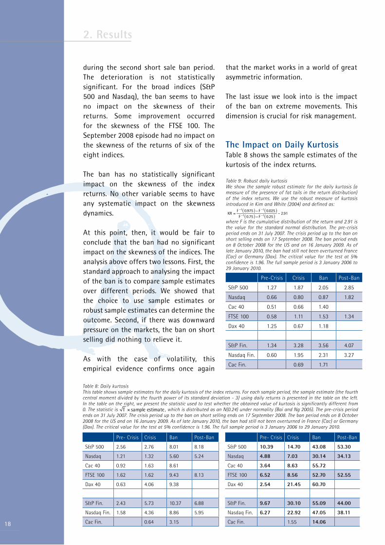
The Impact on Daily KurtosisTable 8 shows the sample estimates of the kurtosis of the index returns.

Table 9: Robust daily kurtosisWe show the sample robust estimate for the daily kurtosis (a measure of the presence of fat tails in the return distribution) of the index returns. We use the robust measure of kurtosis introduced in Kim and White (2004) and defined as:

KR =

F −1 0.975( ) − F −1 0.025( )F −1 0.75( ) − F −1 0.25( )

− 2.91

where F is the cumulative distribution of the return and 2.91 is the value for the standard normal distribution. The pre-crisis period ends on 31 July 2007. The crisis period up to the ban on short selling ends on 17 September 2008. The ban period ends on 8 October 2008 for the US and on 16 January 2009. As of late January 2010, the ban had still not been overturned France (Cac) or Germany (Dax). The critical value for the test at 5% confidence is 1.96. The full sample period is 3 January 2006 to 29 January 2010.

Pre-Crisis Crisis Ban Post-Ban

S&P 500 1.27 1.87 2.05 2.85

Nasdaq 0.66 0.80 0.87 1.82

Cac 40 0.51 0.66 1.40

FTSE 100 0.58 1.11 1.53 1.34

Dax 40 1.25 0.67 1.18

S&P Fin. 1.34 3.28 3.56 4.07

Nasdaq Fin. 0.60 1.95 2.31 3.27

Cac Fin. 0.69 1.71

2. Results

Table 8: Daily kurtosis This table shows sample estimates for the daily kurtosis of the index returns. For each sample period, the sample estimate (the fourth central moment divided by the fourth power of its standard deviation - 3) using daily returns is presented in the table on the left. In the table on the right, we present the statistic used to test whether the obtained value of kurtosis is significantly different from 0. The statistic is T × sample estimate , which is distributed as an N(0.24) under normality (Bai and Ng 2005). The pre-crisis period ends on 31 July 2007. The crisis period up to the ban on short selling ends on 17 September 2008. The ban period ends on 8 October 2008 for the US and on 16 January 2009. As of late January 2010, the ban had still not been overturned in France (Cac) or Germany (Dax). The critical value for the test at 5% confidence is 1.96. The full sample period is 3 January 2006 to 29 January 2010.

Pre- Crisis Crisis Ban Post-Ban Pre- Crisis Crisis Ban Post-Ban

S&P 500 2.56 2.76 8.01 8.18 S&P 500 10.39 14.70 43.08 53.30

Nasdaq 1.21 1.32 5.60 5.24 Nasdaq 4.88 7.03 30.14 34.13

Cac 40 0.92 1.63 8.61 Cac 40 3.64 8.63 55.72

FTSE 100 1.62 1.62 9.43 8.13 FTSE 100 6.52 8.56 52.70 52.55

Dax 40 0.63 4.06 9.38 Dax 40 2.54 21.45 60.70

S&P Fin. 2.43 5.73 10.37 6.88 S&P Fin. 9.67 30.10 55.09 44.00

Nasdaq Fin. 1.58 4.36 8.86 5.95 Nasdaq Fin. 6.27 22.92 47.05 38.11

Cac Fin. 0.64 3.15 Cac Fin. 1.55 14.06

An unambiguous conclusion that can be drawn here is that extreme movements were more frequent during the ban than in the pre-crisis period. For some broad indices (S&P 500, Cac 40) there was a

substantial increase in kurtosis during the ban period. Robust estimates of kurtosis, as shown in table 9, lead to similar conclusions.

2. Results

19

Table 10: The dynamic impact on daily kurtosis of the crisis and the short sale banThis table shows the results of the regression of the daily kurtosis onto the lag of the daily kurtosis, the market index return, the log of the trading volume, and several other control variables. Daily kurtosis is obtained by using a rolling window of the sixty previous days: for each day, we calculated the kurtosis of the returns of the previous sixty days. The legend for table 3 applies here.


S&P 500 Coef. -1.554 -1.013 0.082 -0.067 0.059 -0.123 -0.037 0.106 0.924 -4.908 -20.480

t statistic -1.155 -0.992 1.323 -0.120 0.456 -2.231 -0.337 0.757

Nasdaq Coef. -0.632 -0.727 0.037 -0.091 0.040 -0.046 -0.021 0.186 0.946 -4.167 -21.843

t statistic -0.664 -1.249 0.821 -0.278 0.533 -1.959 -0.329 2.265

Cac 40 Coef. -1.990 1.799 0.116 -0.632 -0.062 -0.030 0.428 0.002 0.943 -4.782 -21.017

t statistic -3.933 3.787 4.222 -2.316 -0.993 -1.366 6.049 0.110

FTSE 100 Coef. -0.625 0.646 0.040 0.000 -0.025 -0.011 0.407 0.036 0.929 -5.404 -21.125

t statistic -1.098 1.252 1.476 0.002 -0.408 -0.588 5.481 1.039

Dax 40 Coef. 0.170 -0.767 -0.649 -0.184 0.032 0.216 -0.022 0.903 -4.230 -25.201

t statistic 3.708 -0.766 -1.151 -1.457 0.744 1.545 -0.515

S&P Fin. Coef. 0.377 0.168 0.091 0.082 -0.095 0.190 0.038 0.887 -6.167 -20.538

t statistic 5.937 0.409 0.222 0.878 -3.107 2.283 0.380

Nasdaq Fin. Coef. 0.265 0.450 -0.032 0.080 -0.049 0.192 0.102 0.922 -4.987 -20.525

t statistic 5.529 1.462 -0.124 1.384 -2.647 3.407 1.617

Cac Fin. Coef. 0.356 1.182 -0.078 -0.253 0.568 -0.048 0.933 -4.412 -13.409

t statistic 5.292 3.081 -0.251 -2.211 6.412 -1.438

Table 11: The dynamic impact on daily robust kurtosis of the crisis and the short sale banThis table shows the results of the regression of the daily robust kurtosis onto the lag of the daily robust kurtosis, the market index return, the log of the trading volume, and several other control variables. Daily robust kurtosis is obtained by using a rolling window of the sixty previous days: for each day, we calculated the robust kurtosis of the returns of the previous sixty days. The legend for table 3 applies here.


S&P 500 Coef. -0.642 0.417 0.033 0.456 -0.033 -0.046 -0.017 -0.012 0.901 -4.635 -21.866

t statistic -1.097 0.932 1.220 1.841 -0.578 -2.028 -0.358 -0.195

Nasdaq Coef. -0.180 0.636 0.009 0.437 -0.065 -0.011 -0.027 0.089 0.949 -3.631 -24.324

t statistic -0.389 2.243 0.435 2.729 -1.752 -1.048 -0.877 2.249

Cac 40 Coef. -0.449 -0.065 0.025 -0.224 -0.009 -0.013 0.012 0.013 0.933 -4.396 -22.561

t statistic -1.286 -0.199 1.328 -1.191 -0.208 -0.866 0.256 0.891

FTSE 100 Coef. -0.313 0.327 0.015 0.243 0.022 0.007 -0.004 0.056 0.943 -4.539 -22.760

t statistic -0.785 0.902 0.814 1.278 0.505 0.488 -0.076 2.242

Dax 40 Coef. 0.024 1.528 0.334 -0.011 -0.011 0.095 0.013 0.937 -4.000 -20.462

t statistic 1.656 3.574 1.403 -0.200 -0.593 1.578 0.695

S&P Fin. Coef. 0.052 -0.005 -0.151 0.065 -0.021 0.004 0.059 0.917 -4.406 -22.432

t statistic 3.479 -0.026 -0.792 1.503 -1.588 0.119 1.260

Nasdaq Fin. Coef. 0.033 0.490 -0.091 0.101 -0.015 0.022 0.114 0.934 -4.075 -22.054

t statistic 3.048 2.423 -0.542 2.652 -1.392 0.678 2.750

Cac Fin. Coef. 0.035 0.185 0.275 0.022 0.048 -0.014 0.888 -3.988 -14.639

t statistic 1.734 0.831 1.516 0.329 1.192 -0.707

20

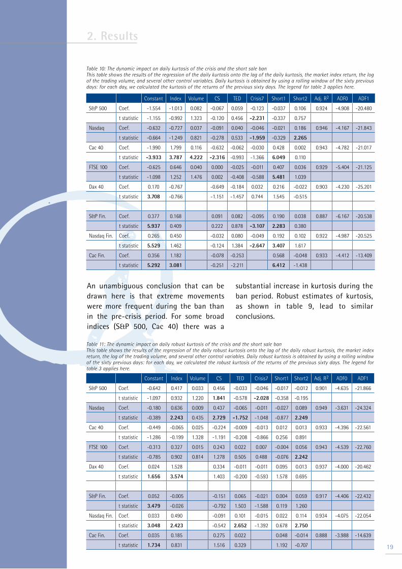
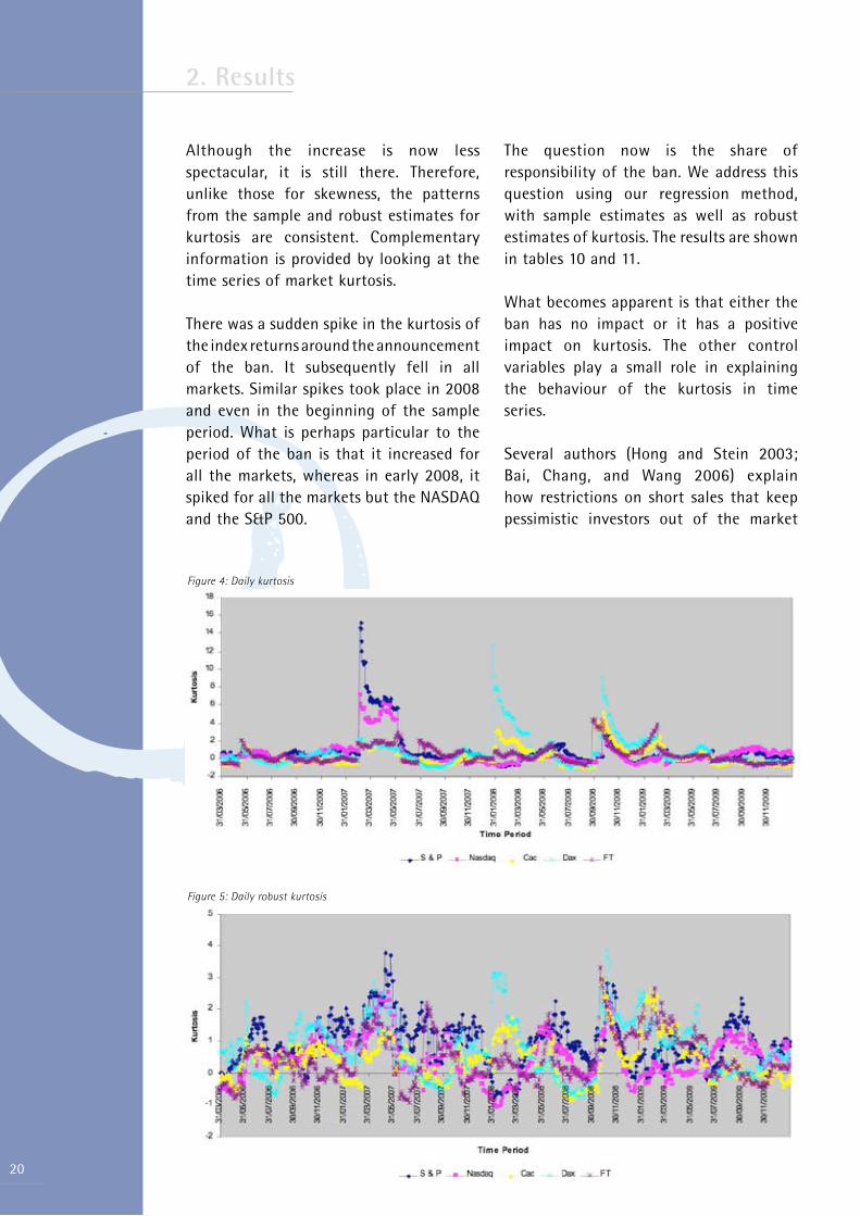
Although the increase is now less spectacular, it is still there. Therefore, unlike those for skewness, the patterns from the sample and robust estimates for kurtosis are consistent. Complementary information is provided by looking at the time series of market kurtosis.

There was a sudden spike in the kurtosis of the index returns around the announcement of the ban. It subsequently fell in all markets. Similar spikes took place in 2008 and even in the beginning of the sample period. What is perhaps particular to the period of the ban is that it increased for all the markets, whereas in early 2008, it spiked for all the markets but the NASDAQ and the S&P 500.

The question now is the share of responsibility of the ban. We address this question using our regression method, with sample estimates as well as robust estimates of kurtosis. The results are shown in tables 10 and 11.

What becomes apparent is that either the ban has no impact or it has a positive impact on kurtosis. The other control variables play a small role in explaining the behaviour of the kurtosis in time series.

Several authors (Hong and Stein 2003; Bai, Chang, and Wang 2006) explain how restrictions on short sales that keep pessimistic investors out of the market

2. Results

Figure 4: Daily kurtosis

Figure 5: Daily robust kurtosis

may result in a market dynamic that leads to severe crashes or at least to discrete negative jumps in stock prices. Our empirical evidence from the financial sector indices on the behaviour of the kurtosis seems to be in line with these conclusions. For other reasons, the market, broadly speaking, also experienced a surge in tail events.

It is worth noting that the hitherto described behaviour of the moments is driven mainly by the actions of investors who, though usually bullish, decided to bail out of the markets. That is, the behaviour of the indices was not affected by the migration of short sellers from the underlying market to the options market; as Battalio and Schultz (2009) show, there was no such migration.

2. Results

21

22

The ban on short selling increased the daily volatilities of the markets; the impact of the ban was greater than the impact of the ongoing financial crisis. Skewness and kurtosis, by contrast, changed over the ban period but for reasons other than the institution of the ban. For individual stocks, increased volatility could be interpreted as an increase in idiosyncratic risk. For the aggregate market, one possible interpretation could be that this excess volatility is the outcome of the fluctuating sentiment of the markets: investors in the markets change their beliefs about future economic prospects too often and thus (over)react to any signal they receive.

What perspective do these findings offer on the SEC’s recent move (late February 2010) to introduce circuit breakers that will trigger bans on shorting stocks whose prices fall by more than 10% in one day? Trading halts in financial markets are most often believed to be effective. Yet the halt must concern all traders, not just short sellers. As it stands, the new regulation means that the pressure will simply come from long bullish investors deciding to bail out of the markets rather than from short sellers.

No such measure has been taken by the regulatory body of the EU since, in several countries (France, for example), short selling is still banned. The February announcement of the EU market authorities simply states the thresholds above which the investors must declare their short sale positions. There seems to be a common belief that such regulation will reduce the opacity of this market. It may well, but it will certainly not make it less concentrated, a failure which means that the problem of the manipulative power of short sellers, if it exists, has still not been tackled. In addition, these differences in regulation may cause a migration of

trading from one market to another and create artificial price discrepancies and thus pseudo-arbitrage opportunities.

These regulatory episodes offer new opportunities for the hedge fund industry. Some strategies could probably exploit the differences in regulation from one country to another. This time, we hope, hedge funds will not be blamed for taking what they are given.

3. Concluding Remarks

• Autore, D., R. Billingsley, and T. Kovacs. 2009. Short sale constraints, dispersion of opinions, and market quality: Evidence from the short sale ban on US financial stocks. Working paper.

• Bai, Y., E. Chang, and J. Wang. 2006. Asset prices under short-sale constraints. Working paper.

• Bai, J., and S. Ng. 2005. Tests for skewness, kurtosis, and normality for time series data. Journal of Business and Economic Statistics 23 (1): 49-60.

• Battalio, R., and P. Schultz. 2009. Regulatory uncertainty and market liquidity: The 2008 short sale ban's impact on equity option markets. Working paper.

• Boehmer, E., C. M. Jones, and X. Zhang. 2008. Unshackling short sellers: The repeal of the uptick rule. Working paper, Columbia University.

• Bowley, A. L. 1920. Elements of statistics. New York: Charles Scribner’s Sons.

• Brunnermeier, M. K. 2009. Deciphering the liquidity and credit crunch 2007–2008. Journal of Economic Perspectives 23:77–100.

• Crow, E. L., and M. Siddiqui. 1967. Robust estimation of location. Journal of the American Statistical Association 62:353-89.

• Diamond, D. W., and R. E. Verrecchia. 1987. Constraints on short-selling and asset price adjustment to private information. Journal of Financial Economics 18:277-311.

• Diether, K. B., K. H. Lee, and I. M. Werner. 2009. It’s SHO time! Short-sale price tests and market quality, forthcoming, Journal of Finance.

• Hong, H., and J. Stein. 2003. Differences of opinion, short-sales constraints, and market crashes. Review of Financial Studies 16:487–525.

• Kim, T., and H. White. 2004. On more robust estimation of skewness and kurtosis. Finance Research Letters 1:56-70.

• Lioui, A. 2009. The undesirable effects of banning short sales. Position paper, EDHEC Risk Institute.

• Marsh, I., and N. Niemer. 2008. The impact of short sales restrictions. Working paper.

• Miller, M. 1977. Risk, uncertainty, and divergence of opinion. Journal of Finance 32:1151-68.

• Purnanandam, A., and N. Seyhun. 2009. Do short sellers trade on private information or false information? Working paper.

References

23

24

2010 Position Papers• Amenc, N., P. Schoeffler, and P. Lasserre. Organisation optimale de la liquidité des fonds d’investissement (March).

2010 Publications• Amenc, N., F. Goltz, and A. Grigoriu. Risk control through dynamic core-satellite portfolios of ETFs: Applications to absolute return funds and tactical asset allocation (January).

• Amenc, N., F. Goltz, and P. Retkowsky. Efficient indexation: An alternative to cap-weighted indices (January).

• Goltz, F., and V. Le Sourd. Does finance theory make the case for capitalisation-weighted indexing? (January).

2009 Position Papers• Amenc, N., and S. Sender. A Welcome European Commission Consultation on the UCITS Depositary Function, a Hastily Considered Proposal (September).

• Sender, S. IAS 19: Penalising changes ahead (September).

• Amenc, N. Quelques réflexions sur la régulation de la gestion d'actifs (June).

• Giraud, J.-R. MiFID: One Year On (May).

• Lioui, A. The undesirable effects of banning short sales (April).

• Gregoriou, G., and F.-S. Lhabitant. Madoff: A riot of red flags (January).

2009 Publications• Sender, S. Reactions to an EDHEC Study on the Impact of Regulatory Constraints on the ALM of Pension Funds (October).

• Amenc, N., L. Martellini, V. Milhau and V. Ziemann. Asset-Liability Management in Private Wealth Management (September).

• Amenc, N., F. Goltz, A. Grigoriu, and D. Schroeder. The EDHEC European ETF survey (May).

• Sender, S. The European pension fund industry again beset by deficits (May).

• Martellini, L., and V. Milhau. Measuring the benefits of dynamic asset allocation strategies in the presence of liability constraints (March).

• Le Sourd, V. Hedge fund performance in 2008 (February).

• La gestion indicielle dans l'immobilier et l'indice EDHEC IEIF Immobilier d'Entreprise France (February).

• Real estate indexing and the EDHEC IEIF Commercial Property (France) Index (February).

• Amenc, N., L. Martellini, and S. Sender. Impact of regulations on the ALM of European pension funds (January).

• Goltz, F. A long road ahead for portfolio construction: Practitioners' views of an EDHEC survey. (January).

EDHEC Risk Institute Position Papers and Publications (2007-2010)

2008 Position Papers • Amenc, N., and S. Sender. Assessing the European banking sector bailout plans (December).

• Amenc, N., and S. Sender. Les mesures de recapitalisation et de soutien à la liquidité du secteur bancaire européen (December).

• Amenc, N., F. Ducoulombier, and P. Foulquier. Reactions to an EDHEC study on the fair value controversy (December). With the EDHEC Financial Analysis and Accounting Research Centre.

• Amenc, N., F. Ducoulombier, and P. Foulquier. Réactions après l’étude. Juste valeur ou non : un débat mal posé (December). With the EDHEC Financial Analysis and Accounting Research Centre.

• Amenc, N., and V. Le Sourd. Les performances de l’investissement socialement responsable en France (December).

• Amenc, N., and V. Le Sourd. Socially responsible investment performance in France (December).

• Amenc, N., B. Maffei, and H. Till. Les causes structurelles du troisième choc pétrolier (November).

• Amenc, N., B. Maffei, and H. Till. Oil prices: The true role of speculation (November).

• Sender, S. Banking: Why does regulation alone not suffice? Why must governments intervene? (November).

• Till, H. The oil markets: Let the data speak for itself (October).

• Amenc, N., F. Goltz, and V. Le Sourd. A comparison of fundamentally weighted indices: Overview and performance analysis (March).

• Sender, S. QIS4: Significant improvements, but the main risk for life insurance is not taken into account in the standard formula (February). With the EDHEC Financial Analysis and Accounting Research Centre.

2008 Publications• Amenc, N., L. Martellini, and V. Ziemann. Alternative investments for institutional investors: Risk budgeting techniques in asset management and asset-liability management (December).

• Goltz, F., and D. Schröder. Hedge fund reporting survey (November).

• D’Hondt, C., and J.-R. Giraud. Transaction cost analysis A-Z: A step towards best execution in the post-MiFID landscape (November).

• Amenc, N., and D. Schröder. The pros and cons of passive hedge fund replication (October).

• Amenc, N., F. Goltz, and D. Schröder. Reactions to an EDHEC study on asset-liability management decisions in wealth management (September).

• Amenc, N., F. Goltz, A. Grigoriu, V. Le Sourd, and L. Martellini. The EDHEC European ETF survey 2008 (June).


25

26

• Amenc, N., F. Goltz, and V. Le Sourd. Fundamental differences? Comparing alternative index weighting mechanisms (April).

• Le Sourd, V. Hedge fund performance in 2007 (February).

• Amenc, N., F. Goltz, V. Le Sourd, and L. Martellini. The EDHEC European investment practices survey 2008 (January).

2007 Position Papers • Amenc, N. Trois premières leçons de la crise des crédits « subprime » (August).

• Amenc, N. Three early lessons from the subprime lending crisis (August).

• Amenc, N., W. Géhin, L. Martellini, and J.-C. Meyfredi. The myths and limits of passive hedge fund replication (June).

• Sender, S., and P. Foulquier. QIS3: Meaningful progress towards the implementation of Solvency II, but ground remains to be covered (June). With the EDHEC Financial Analysis and Accounting Research Centre.

• D’Hondt, C., and J.-R. Giraud. MiFID: The (in)famous European directive (February).

• Hedge fund indices for the purpose of UCITS: Answers to the CESR issues paper (January).

• Foulquier, P., and S. Sender. CP 20: Significant improvements in the Solvency II framework but grave incoherencies remain. EDHEC response to consultation paper n° 20 (January).

• Géhin, W. The Challenge of hedge fund measurement: A toolbox rather than a Pandora's box (January).

• Christory, C., S. Daul, and J.-R. Giraud. Quantification of hedge fund default risk (January).

2007 Publications• Ducoulombier, F. Etude EDHEC sur l'investissement et la gestion du risque immobiliers en Europe (November/December).

• Ducoulombier, F. EDHEC European real estate investment and risk management survey (November).

• Goltz, F., and G. Feng. Reactions to the EDHEC study "Assessing the quality of stock market indices" (September).

• Le Sourd, V. Hedge fund performance in 2006: A vintage year for hedge funds? (March).

• Amenc, N., L. Martellini, and V. Ziemann. Asset-liability management decisions in private banking (February).

• Le Sourd, V. Performance measurement for traditional investment (literature survey) (January).


EDHEC Risk Institute is part of EDHEC Business School, one of Europe’s leading business schools and a member of the select group of academic institutions worldwide to have earned the triple crown of international accreditations (AACSB, EQUIS, Association of MBAs). Established in 2001, EDHEC Risk Institute has become the premier European centre for applied financial research.

In partnership with large financial institutions, its team of 47 permanent professors, engineers and support staff implements six research programmes and ten research chairs focusing on asset allocation and risk management in the traditional and alternative investment universes. The results of the research programmes and chairs are disseminated through the three EDHEC Risk Institute locations in London, Nice and Singapore.

EDHEC Risk Institute validates the academic quality of its output through publications in leading scholarly journals, implements a multifaceted communications policy to inform investors and asset managers on state-of-the-art concepts and techniques, and forms business partnerships to launch innovative products. Its executive education arm helps professionals to upgrade their skills with advanced risk and investment management seminars and degree courses, including the EDHEC Risk Institute PhD in Finance and the EDHEC Risk Institute Executive MSc in Risk and Investment Management.

Copyright © 2010 EDHEC Risk Institute

For more information, please contact: Carolyn Essid on +33 493 187 824 or by e-mail to: [email protected]

EDHEC Risk Institute393-400 promenade des AnglaisBP 311606202 Nice Cedex 3 - France

EDHEC Risk Institute—EuropeNew Broad Street House - 35 New Broad StreetLondon EC2M 1NHUnited Kingdom

EDHEC Risk Institute—Asia9 Raffles Place#57-12 Republic PlazaSingapore 048619

www.edhec-risk.com

Institute

393-400 promenade des anglais web:...

Documents