Who decides on trade policy? ∗

Joachim Jarreau†

May 9, 2014

Abstract

This paper studies the impacts and determinants of trade policy. Using

detailed panel data on applied tari� protection, I estimate sector-level trade

elasticities, then calibrate a structural gravity model of world trade and com-

pute the impacts of trade policy over 2001-2007. I compute the impacts of

trade agreements which were applied and of those which were not. I �nd that

the expected market access gains, re�ected in domestic mill price increases,

is a stronger determinant of the signing of PTAs than the real income gains

expected by countries. This result suggests that distortions exist in the set-

ting of trade policy. I also �nd that larger expected gains from multilateral

liberalization reduce the probability to engage in preferential agreements.

Keywords: International trade, Preferential trade agreements, Counter-

factual Estimation, Trade creation and diversion.

JEL classi�cation: F13, F12, F47.

∗I would like to thank James Anderson, Scott Baier, Lionel Fontagné, Nuno Limao, DanielMirza, Marcelo Olarreaga, Joao Santos Silva, Vincent Vicard and participants at GSIE seminarat Paris 1 University and RIEF conference at Bocconi University for very helpful comments anddiscussions.†Aix-Marseille school of economics (joachim.jarreau@gmail.com).

1 Introduction

Preferential trade agreements (PTAs) are growing fast in number, while multilateral

trade negotiations are stalling. From 1995 through 2010, the number of PTAs in-

creased fourfold to reach 300 PTAs presently in force (WTO, 2011); the geographical

coverage of PTAs has expanded both within and between continents, and with the

participation of developed and developing countries. At the same time, negotiations

to open trade multilaterally have not made signi�cant progress in recent years.

Given the non-optimality of preferential trade liberalization, and the distorsions

associated to it, these facts are worrying. They raise the question of why coun-

tries favor discriminatory trade opening, when theory suggests a unilateral and non-

discriminatory opening of trade to be optimal. We examine this question by looking

at the immediate gains countries may expect from alternative trade policies. These

gains are of two types: market access gains, which translate into higher production

prices, and real income gains, which bene�t consumers by lowering the domestic

price index. Our results show that the former are a stronger determinant of trade

policy than the latter.

Our approach consists in letting the data on trade policies talk about what guides

countries' decisions. We use an exhaustive database of tari� protection for the period

2001-2007, and rely on a simple Armington model of international trade to compute

the implied changes in trade and real income for world countries.

First, we characterize each country's trade policy in our period of interest, mea-

suring the impacts of its policy all else equal. We ask in particular if these trade

policies tend to reinforce distorsions in the trade structure of countries, by making

trade more preferential. Results show disparities across countries: about half the

countries in our sample have had a policy which made their trade more multilateral,

all else equal. This runs counter to the intuition that the overwhelming trend in re-

cent years has been toward more preferentialism, as suggested by the multiplication

of PTAs. Rather, our analysis suggests that some countries tend to favor one or the

other modes of liberalization, depending on the relative gains they expect from each

process.

2

This observation naturally leads us to ask about the determinants of trade policy

choices of countries. What explains that countries choose to engage in PTAs, or to

open trade in a non-preferential manner? Previous literature has emphasized that

the choice of trade policy results from confronting di�erent interests (Grossman and

Helpman, 1995): producers in di�erent sectors tend to favor or oppose an agreement

depending on the structure of protection and productivity di�erences between po-

tential partners, causing them to expect market access gains, or increased import

competition. Consumers expect real income gains through lower prices, however

they may also expect losses by diversion if distorsions in the tari� structure become

important. Computing the impacts of alternative trade policy choices for produc-

ers and for consumers, we confront these impacts with the list of actually signed

agreements. Results indicate that expected real income gains from signing a PTA

predict those agreements that were actually signed; moreover, potential gains from

multilateral opening reduce the probability of signing, which con�rms the existence

of a tradeo� between the two modes of liberalization. However, we also �nd that

the two gains do not carry the same weight in a country's trade policy: gains in

production prices have an impact that is about two times larger on the probability

of signing.

Finally, we also show that the losses by diversion faced by countries are also a

signi�cant predictor of the signing of PTAs, which con�rms a contagion or �domino

e�ect� (Baldwin, 1993) being one of the main forces behind the proliferation of PTAs.

In other words, countries sign PTAs also for the motive of avoiding the losses from

non-preferential access to a partner's market.

Our approach focuses on terms-of-trade impacts of trade policy. By using a multi-

sector, endowment model of international trade with Armington di�erentiation, we

restrict the analysis to the short-term e�ects of trade barrier changes, leaving aside

longer-term e�ects through adjustments of the production structure or technology

improvements. Previous literature has shown these terms-of-trade motives to be

predominant in driving trade policy (Baier and Bergstrand, 2004). Our results

con�rm this aspect, and more importantly, show that structural estimates of terms-

of-trade have explanatory power for trade policy, above and beyond proxies based

3

on distance and income levels. The use of the Armington endowments model is also

justi�ed by its good performance to explain trade data (Anderson and Yotov, 2010b,

2012).

We �rst present the model and its relation to other models belonging to the

�structural gravity� class. We then analyze in a simple example how the impact of

preferential tari� reductions on prices and real income varies with the trade elas-

ticity, the relative size of trading partners and pre-FTA trade patterns. Then, we

parameterize the model to quantify PTA e�ects, which boils down to estimating

sector-level trade elasticities. This parameter is crucial as it is a su�cient statistic

which allows to predict the adjustment of trade and prices to trade policy shocks,

in structural gravity models. We estimate these parameters using disaggregated

bilateral applied tari� panel data, which allows to control for the endogeneity of

trade policy through the use of country-sector �xed e�ects (Baier and Bergstrand,

2007). Once armed with these elasticity estimates and with our data on applied tar-

i� changes, we compute PTA e�ects by counterfactual estimation. This allows us to

compute the trade and real income impacts implied trade policies as implemented by

world countries during the period. Then, we use the method to confront the e�ects

of actual trade policies to those of alternative policies, namely trade agreements and

multilateral trade liberalizations.

A large literature has studied the determinants of trade policy. The seminal

paper by Grossman and Helpman (1995) builds a political economy framework where

governments take into account both voter's interests and industry special interests

in deciding over trade agreements. By contrast, we do not enter into the political

economy structure of countries, as we do not observe whether groups are organized

into lobbies, nor whether there is coordination across sectors in trying to in�uence

trade policy. Rather, we make the implicit hypothesis that net gains to each group,

aggregated across sectors, should matter for the government's decisions. This should

be the case if the possibility of transfers across groups exists, so that adversely

impacted groups can be compensated for their losses. Our results indicate that this

is the case only in part. Our results are also related to those in Goldberg and Maggi

(1999), who run an empirical test of the model by Grossman (1994). These authors

4

quantify the weight of welfare in the US government's objective function and �nd

it to be very close to 1 (0.99), implying that the US government is close to being a

perfect welfare maximizer in its design of tari� structure. By contrast, our analysis

based on the signing of PTAs �nds robust evidence that world countries' trade

policies substantially di�er from the welfare-maximizing, overweighting producers'

interests over those of consumers.

The use of an endowments model of trade based on Armington di�erentiation

and Dixit- Stiglitz preferences places our paper in the so-called �structural gravity�

literature (Anderson and Yotov, 2011; Egger et al., 2011)). It has been recognized

that di�erent one-sector models of trade, based on CES preferences, such as Krug-

man (1979); Eaton and Kortum (2002); Melitz (2003) have in common to generate

a gravity equation with a similar structure for trade �ows. One consequence is that

these models generate the same functional form for the impacts of trade cost changes

on prices and real income levels, conditional on trade elasticities and on initial trade

levels (Arkolakis et al., 2012). Thus, estimating trade elasticities becomes the key to

predict price movements in these models, as this parameter encompasses the di�er-

ent margins of adjustment described in these models. This motivates our approach,

which consists in estimating sector-level trade elasticities, in order to compute the

impacts of various trade policy scenarios on price and real income levels. The valid-

ity of these results beyond the Armington model will be discussed in detail in the

text.

In addition, relying on sector-level elasticity estimates instead of a single PTA

parameter allows us to account for heterogeneity in PTA e�ects due to the width

and depth of tari� reductions.1

Finally, by assuming �xed endowments the model features an inelastic export

supply curve, similarly to models of terms-of-trade manipulation and optimal tari�s

(Broda, Limao and Weinstein, 2008, Ludema and Mayda, 2011). Therefore, as

in these models, there is a positive association between market power and tari�s:

1Another di�erence is that we solve the model in full general equilibrium, allowing for exportprices to a�ect trade through countries' income, contrary to antecedents in which trade changesare computed while implicitly keeping countries' income as �xed (Anderson and Wincoop, 2003;Anderson and Yotov, 2010a; Baier and Bergstrand, 2009; Egger et al., 2011).

5

countries have an incentive to set higher tari�s on imports from partner countries in

which their market share is higher, while opening trade in priority with those where

their market power is lower.2

The rest of the paper is as follows. In section (2), we present the model, and

discuss its relation to the class of structural gravity models, and the possible gener-

alization of our results in this framework. We then use a simple, 3-country version

of the model to analyze its implications for the e�ects of PTAs on trade, real income

and welfare. In section (4), we estimate the trade elasticities. In section (5), we

compute the price and real income impacts of trade policy implemented by world

countries during our period of study. Then, in section (6), we study the determinants

of the signing of PTAs. Section (7) concludes.

2 Model

This section presents the multi-sector Armington model, and the method used to

calibrate it and to solve it in comparative statics simulation exercises. We then

discuss the relationship between this model and other models of trade featuring

additional margins of adjustment to trade cost changes, such as the Krugman (1979),

Eaton and Kortum (2002) and Melitz (2003) models. We make the point that the

changes in prices and real income levels which we compute in our model can, under

some conditions, be generalized to these richer frameworks.

Model structure

The model features multiple sectors, covering agriculture, mining and manufacturing

activities.3 We model preferences with a Cobb-Douglas structure across sectors and

CES (constant elasticity of substitution) across varieties within each sector. Goods

in each sector k are produced using a speci�c factor, of which each country i has a

2However, contrary to those models, there is no optimal positive tari�, because the gain toconsumers always dominates over losses to domestic producers. This is due to the hypothesis ofimperfect substitution between domestic and imported goods. Thus, issues related to negotiationsover tari�s are not considered here.

3In the empirical application, each sector corresponds to one code in revision 3 of the Interna-tional Standard Industrial Classi�cation (ISIC), maintained by the UN.

6

�xed endowment Lik. Within each sector, we make the Armington assumption that

goods are di�erentiated by country of origin (consumers perceive varieties produced

in di�erent countries as imperfect substitutes).

Demand is thus given by:

ckij = (pki )−σk .

(τ kijP kj

)1−σk

.Ekj , (1)

where ckij is the demand of country j's consumers for the i variety of good k, pki is

the f.o.b (free on board) price of that variety, τ kij is the iceberg trade cost on trade

from i to j in sector k (which is to include geographic and trade policy components

of trade costs), P kj is country j's price index in that sector and σk is the elasticity of

substitution between varieties of that good. Ekj is country j's expenditure on good k,

given by Ekj = αk.Yj, where αk is the Cobb-Douglas parameter share of expenditure

on good k and Yj is country j's total income4.

Sectors are thus modeled as largely independent in the model: labor cannot be

reallocated across sectors, and consumers spend a �xed share of their expenditure

on each sector (Cobb-Douglas assumption)5. We thus abstract from factor-based

comparative advantage e�ects, as well as from inter-sectoral linkages (e.g. vertical

relations). One reason for doing this is that, as documented below, results on price

responses to trade cost changes in the one-sector Armington model are, under some

conditions, valid under a larger class of one-sector models. This is still true of

price responses in each sector of our model, which functions like a superposition of

one-sector Armington models. This restrictive assumption allows to estimate price

responses to trade policy changes using a limited list of statistics (trade elasticity,

trade levels, tari� changes); which would not be possible if accounting for inter-

sectoral linkages.

4Note: parameters of the demand function αk and σk are assumed to be identical across coun-tries.

5This modeling choice is motivated by the fact that our sectors (as de�ned by ISIC codes) aresu�ciently distinct to allow little substitution.

7

The nominal bilateral trade �ow between i and j in sector k is given by

Xkij =

(pki .τ

kij

P kj

)1−σk

.Ekj . (2)

with P kj the ideal price index for j's consumers in country k, given by:

(P kj )(1−σk) =

∑i

(pki .τkij)

1−σk . (3)

A quantity Qki of good k is produced by a representative �rm in country i, using

a speci�c factor Lki which is in �xed supply. Without loss of generality, one can set

the factor requirement to 1, which yields identity between sector-level wages wki and

the f.o.b. price of the good:

wki = pki (4)

The market clearing condition for each variety of each good is written as:

∑j

Xkij = pki .Q

ki , (5)

where the sum is over all destinations, including domestic sales of the good.

Finally, each country's total income Yj is equal to the total value of sales in all

sectors:

Yj =∑k

pkj .Qkj (6)

The structural gravity equation

Anderson and Wincoop (2003) de�ne the aggregate of demand-weighted trade costs

faced by an exporter as the exporter's `multilateral resistance'. This multilateral

price (we use here both terms interchangeably) is de�ned as:

(Πki )

1−σk =∑j

(τ kijP kj

)1−σk Ekj

Y kw

, (7)

8

where Y kw is the total nominal value of world production of good k: Y k

w =∑i p

kiQ

ki .

Using this de�nition and equation 5, one obtains the relationship between f.o.b prices

and multilateral resistance terms as:

(pki )σk =

Y kw

Qki

.(Πki )

1−σk . (8)

Combining this expression with the trade demand equation 2, one obtains the

gravity equation for nominal trade �ows:

Xkij =

(τ kij

P kj Πk

i

)1−σk

.Ekj Y

ki

Y kw

. (9)

which expresses bilateral trade as a function of bilateral trade costs, multilateral

prices (Πki ) and (P k

j ) (labeled exporter and importer multilateral resistance terms,

respectively, by Anderson and Wincoop (2003)), and the income and expenditure

levels of the exporter and importer, Ekj and Y k

i .

One advantage of this expression is that its structure is common to distinct

trade models. More precisely, trade models such as Krugman (1979), Eaton and

Kortum (2002) and Melitz (2003), all yield a �gravity equation� for trade, where

bilateral trade �ows are a constant-elasticity function of bilateral trade costs and of

multilateral price terms for the exporting and importing countries. Across models,

the trade elasticity (equal to 1 − σk in the case considered here) will depend on

di�erent parameters of the model.6

Thus, the trade elasticity can be estimated using equation 9, using a measure of

time-varying bilateral trade costs and country-sector �xed e�ects which control for

the exporter and importer terms P kj and Ek

j , Πki and Y k

i . This obtained estimate

of the trade elasticities, σk, should thus be viewed not as speci�c to the Armington

used here, but valid under more general assumptions which are compatible with the

structural gravity equation.

In turn, the relative price changes in response to trade cost changes, are also

6For example, in the Armington model used here, as in the Krugman (1979) model, it is simplya function of the CES elasticity of substitution. In Eaton and Kortum (2002) and in Melitz(2003), it depends on the CES elasticity and on the parameter governing the distribution of �rmsproductivities.

9

invariant across a class of models, conditional on the value of trade elasticities and

initial trade values. This motivates our empirical strategy: we �rst estimate sector-

level trade elasticities, then compute price and income changes resulting from trade

cost changes (preferential agreements), in a comparative statics exercise whose va-

lidity extends beyond the Armington model. This result is discussed in the section

2.1.

Resolution method Once estimates of the trade elasticities for each sector are

obtained (section 4), the comparative statics exercises in sections 5 and 6 are carried

by solving the model �rst in the reference year 2001 with data for applied tari�s in

that year and total production by country and sector7; then in alternative scenarios

where changes in tari�s are applied, while production values and non-tari� com-

ponents of trade costs are maintained constant. For each set of tari� values, the

model is solved using an iteration algorithm. Equations 8, 3 and 6 are solved in

the variables pki , Pkj and Yj, iterating until the relative error in each component of

the equations is lower than 0.1%. The system admits a unique equilibrium once a

normalization is imposed: we set Yw =∑j Yj = 1.

In each scenario, changes in prices and income levels are then measured as the

relative change between the equilibrium in benchmark year 2001 and the new equi-

librium after tari� changes are applied.

2.1 Validity of our results in more complex models

Results for relative price changes in response to trade cost changes, obtained in the

Armington model presented above can be generalized to a broader class of models

of trade. The basic intuition behind this result is that a number of one-sector

models of trade generate trade equations with the same �gravity� structure for the

trade equation, where the trade elasticity - the elasticity of trade with respect to

trade costs and wages - is a function of di�erent parameters of the model, re�ecting

di�erent margins of adjustment to trade shocks.

In turn, changes in the f.o.b. prices of variety and the ideal price index in each

7See section 4 for details on the data used.

10

country, resulting from a change in trade costs, will be driven by the constant-

elasticity dependence of trade to prices. Thus, the relative changes in prices, con-

ditional on the trade elasticity (as well as on initial trade levels) will be unchanged

across these models. Note that this does not imply equivalence across these models,

but rather, that the trade elasticity is a su�cient statistic to compute a number of

price changes.

Arkolakis et al. (2012) present a set of conditions de�ning a class of models

where this result holds. These include the Krugman (1980) model of trade with

symmetric �rms in monopolistic competition in each country; the Eaton and Kortum

(2002) model of Ricardian comparative advantage, and the Melitz (2003) model with

heterogeneity in �rm productivity.

The three required �macro-level restrictions� are: that trade is balanced; that

the share of pro�ts in a country's total revenues is constant; and that the import

demand system is of the form:

Xij =ξij.Ni.(wiτij)

ε. Yj∑′i ξi′j.N

′i .(w

′iτi′j)

ε(10)

where Xij is trade value from country i to j, Ni is the number of �rms operating

in country i, ξij is a function of parameters distinct from τ ; Yj is country j's income

level; and ε is the �trade elasticity�, which is a function of di�erent parameters in

di�erent models 8

It is relatively straightforward to show that this set of conditions leads to the

following system of equations:

wi =∑l

λilwlYl(wiτil)ε

Yi∑r λrl(wrτrl)ε

(11)

and8Condition 10 is called R3' in Arkolakis et al. (2012) and is more restrictive than condition

R3 under which their most central result on the welfare gains from trade is derived. This centralresult states that welfare change from a shock to trade costs, conditional on the change in import

penetration, is constant across a class of models. This does not mean that these models generatethe same welfare changes from a given trade policy shock, as the import penetration reaction candi�er across models. Thus, in order to derive the stronger result, of interest to us, that relativeprice changes, for a given shock on trade costs, are invariant, condition R3' is necessary.

11

Pj = [∑i

λij(wiτij)ε]−1/ε (12)

where z denotes the ratio of �nal to initial value of variable z, z′/z, resulting

from a arbitrary change in trade costs; and λij = Xij

Ejis the initial share of imports

from i in country j's total expenditure.

This system de�nes the relative change in wages wi as an implicit function of

initial trade shares and relative changes in trade costs.

Our Armington model of trade veri�es these assumptions: trade is balanced;

pro�ts are zero, due to the hypothesis of perfect competition; and trade �ows are

given by the expression 10, with the number of �rms and the parameter ξ being

uniformly one; and ε = 1− σ, with σ our CES elasticity of substitution.

This ensures that the relative changes in wages (or equivalently, f.o.b. prices) wi

and in the consumption price index Pj are given by conditions 11 and 12, in this

class of models, and thus that these changes, conditional on trade elasticities and

trade shares, are invariant across these models.

These models include some of the models often used in the trade literature.

One important common characteristic of these models is that they assume CES

preferences9. In particular, this implies that markups will be constant: pro- or

anti-competitive e�ects of trade openness are thus not accounted for.10

3 Impact of a PTA on prices: a simple example

In this section, we use a simple example with a three-country, one-sector version of

the Armington model, to illustrate the impacts of preferential trade liberalization

on production prices and real income in this model.

We consider the following stylized model with three countries denoted A, B and

C, producing and trading di�erentiated varieties of the same one good. We assume

9In principle, condition 10 does not imply that preferences are CES, as this condition charac-terizes the import demand function as a result of both preferences and supply side responses. Inpractice, commonly used models verifying 10 all assume CES preferences.

10See e.g. Neary and Mrazova (2013) for a discussion of the relation between demand elasticitiesand pro-competitive e�ects in a more general framework.

12

that A is at an equal distance from B and C, with a larger distance between B and

C. In practice, we set initial trade costs as:

τij = 1 if i = j

τAB = τAC = 1.5

τBC = 2

tradecostij = (1 + AV ij).τij (13)

where AV is the ad-valorem equivalent of trade policy barriers applied by j

on imports from i. That is, bilateral trade costs result from a combination of a

�geographical� component and of policy barriers applied by countries.11

We initially set the size of countries A, B, C to 1, 10 and 5; a country's size being

here equal to its labor endowment, or equivalently to the volume of its production.

We assume that countries initially apply a MFN, non-discriminatory tari� to all

imports, and set it to 30%. We consider the case of a bilateral PTA signed between

countries A and B, which sets tari�s between these two countries to 0.

We focus on the impact of the PTA on prices in country A. The questions of

interest to us, here and in the rest of the paper, are the impact of the PTA on the

producer price pA; the consumer price index PA; and the country's real income YA =

pA.QA

PA.12

Figure 1 represents the relative change in production price pA: we have here two

parameters varying, the size of the partner country B, which goes from 1 to 20; and

the elasticity of substitution σ, which varies between 1 and 10.

The �gure shows that the impact of the PTA on production price changes sign

11This is similar to the functional form which will be used to model trade costs in the empiricalpart, where the geographic component will account in particular for distance and contiguity.

12In the case of policy barriers being in the form of tari�s, the real income of a country includes

the share of revenues from trade barriers which is rebated:YA =pA.QA+ρ.

∑i=B,C

AViXiA

PAwith ρ the

share of revenue rebated. We will check that modifying ρ does not modify qualitatively our results.

13

depending on these two parameters. In particular, in the low substitution case,

the impact is positive, while it becomes mostly negative in the high-σ region. This

re�ects two competing e�ects: on one hand, the PTA grants preferential access to

country B's market, which allows A's producers to raise their production price, the

more so, the more inelastic the demand for their variety is. On the other hand, the

PTA entails reciprocal tari� reductions, which implies a competition e�ect on A's

domestic market: this tends to bring the price of A's variety lower, with this e�ect

being larger if competing varieties from A and B are more substitutable.

These two e�ects are generally larger when the size of the partner country in-

creases. Thus, in a low-σ sector, one would expect producers in country A to prefer a

PTA with a large partner (all else equal); while in a high-σ where import competition

dominates, they would prefer a PTA with a smaller partner country.

Figure 2 displays the impact of the PTA on country A's consumer price index

(the CES ideal price index). The impact is negative as the PTA lowers the aggregate

price of consumption in the country; it is displayed in absolute value here. The �gure

shows that consumers stand to gain from the PTA, the more so when σ is low and

the size of the partner country increases. Interestingly, the gradient of the impact

is not aligned with that of the production price impact: for example, in the high-σ

region, the gain increases with the partner's size, while the impact on production

price becomes more negative. This illustrates the divergence of interests in trade

policy: in a country trading a good with high trade elasticity, a policy focused on

maximizing production prices would prefer a PTA with a small partner country,

while favoring the gains to consumers would lead to choose a PTA with a large

country.

Figure 3 displays the impact of the PTA on country A's real income. It shows

that the larger gains in real income are obtained in the high-σ, high-Q region. The

PTA lowers the consumer price index in country A, through cheaper imports from

partner country B and through the import competition e�ect, which also lowers the

domestic variety's price. These e�ects are larger in the high-σ region and dominate

the negative impact on domestic prices, causing a larger real income gain. This

illustrates the divergence between the objectives of maximizing production prices

14

versus real income.

010

20

0246810−0.04

−0.03

−0.02

−0.01

0

0.01

0.02

0.03

0.04

Q

PTA impact on production price

sigma

Rel

ativ

e pr

ice

chan

ge

Figure 1: PTA impact on country A's production price

0

10

20

02468100

0.02

0.04

0.06

0.08

0.1

0.12

0.14

0.16

Q

PTA impact on price index (abs. value)

sigma

Rel

ativ

e pr

ice

chan

ge

Figure 2: PTA impact on country A's consumer price index

Another example of this divergence is given on �gure 4, which focuses on changes

in production prices and in the consumer price index, in the case σ = 8, as a function

of the partner country's size Q. The �gure highlights the non-linearities in price

15

0

10

20

02468100

0.05

0.1

0.15

0.2

0.25

Q

PTA impact on Real income

sigma

Rel

ativ

e pr

ice

chan

ge

Figure 3: PTA impact on country A's real income

changes in this model and shows that the maxima of the two price functions do not

coincide.

This highlights again the divergence between the two objectives: assuming that a

country would face the alternative of signing a PTA with two countries di�ering only

by their size, the optimal choice would di�er depending on whether policymakers

favor the objective of maximizing production prices, or consumers' real income level.

The rest of the paper will attempt to use the information on the PTAs signed

by world countries as indicative of the underlying objective pursued by signing gov-

ernments. The same Armington model, but with more countries, multiple sectors

will be used. Variations in initial trade level and sectoral composition, distance to

potential PTA partners and third countries, will generate variations in the potential

impact of a PTA on signing countries' production prices and real income. Our ap-

proach consists in confronting these impacts to the observed choice of PTAs to infer

information on the objective functions governing trade policy choices.

16

0 5 10 15 20 25 30 35 40−0.035

−0.03

−0.025

−0.02

−0.015

−0.01

−0.005

0

0.005

Size of partner country

Rel

ativ

e pr

ice

chan

ge

PTA impact on price index, production price

prod. price impactPrice index impact

Figure 4: Incidence on importer's price index

17

4 Estimation of sector elasticities

Empirical speci�cation The estimation of the e�ects of PTAs is done in two

steps. In this section we estimate elasticities of substitution at sector level to

parametrize the model. Next we estimate the e�ects of trade policy changes. Taking

the log of equation (9) yields

lnXkij = ln

Y ki

Y kW

+ lnEkj

Y kW

+ (1− σk).(ln τ kij − ln(P kj .Π

ki )). (14)

A functional form of trade costs is needed to estimate this equation. In line with

the common practice in the literature, we assume the following log-linear stochastic

form:

τ kij = (1 + Tari�kij).dρk

ij .eαkContigij .eβ

kComlangij .eukij , (15)

where Tari�kij is the ad-valorem equivalent of tari� barriers on i's products exported

to j in sector k, dij is the distance between i and j and ukij represent unobserved

bilateral trade cost determinants. We also add two dummy variables: Contigij,

which is unity if countries/regions i and j are contiguous, and Comlangij, which is

unity if i and j share an o�cial language.

Plugging the functional form of trade costs into (14) and adding time subscripts

to stress the point that some of the variables are time varying give us:

lnXkijt = ln

Y kit

Y kWt

+ lnEkjt

Y kWt

+ (1− σk).(ln(1 + Tarifkijt)− ln(P kjt)− ln(Πk

it))

+ (1− σk).(ρk.dij + αContigij + βComlangij) + εkijt, (16)

where εkijt is the stochastic error term. We estimate this equation separately for

each sector. We introduce exporter-time (λit) and importer-time (λjt) �xed e�ects,

which enables us to control fully for unobserved sector-level country shares of world

production and expenditure, as well as for country multilateral price terms for each

sector. Thus our speci�cation is the following:

lnXkijt = βk ln(1+Tari�kijt)+γ

k ln dij+δkContigij+η

kComlangij+λit+λjt+εkijt. (17)

18

In this equation, coe�cient βk gives us directly the estimate of (1− σk), while γ

gives us the estimate of the product (1− σk).ρk, of which we can deduce ρ; we can

similarly obtain the e�ects of contiguity and common language on trade costs.

Data We estimate the sector-level gravity equation using nominal bilateral trade

values from the BACI trade database.13 Trade data at product Harmonized System

(HS)-6 digit level are aggregated at the International Standard Industrial Classi�-

cation (ISIC) rev.2 level (79 sectors). We see this level of aggregation as consistent

with the de�nition of sectors in the model.14 All world trade is considered, aggre-

gating �ows into 68 countries/regions to keep the model tractable. This estimation

strategy, which reduces the high dimensionality of data, is common in the literature

(see Anderson and van Wincoop, 2003 and Anderson and Yotov, 2010).

Data on distance, contiguity and languages are taken from the distance CEPII

database.15 Tari� data are obtained from the CEPII MacMap database (Bouet et

al., 2008). This data set contains data on bilateral applied tari� protection for the

years 2001, 2004 and 2007. Data on ad-valorem and speci�c tari�s, and on tari�

quotas, are converted into ad-valorem equivalents using unit values data for the

year 2001. Thus, our tari� variable is a comprehensive measure of applied tari�

protection, which enables us to track changes in tari� protection due to preferential

agreements.16 Importantly, this enables us to observe precisely the content of PTAs,

and to observe variations across PTAs in sector coverage, extent of tari� reductions

and time period of implementation.17 Note that running our estimates on three-year

intervals allows us to obtain stable estimates, while the use of yearly data has been

shown to yield unstable gravity estimates, due to delays in the adjustment to trade

13The BACI trade data set is built by the CEPII (see www.cepii.fr/anglaisgraph/bdd/baci.htm).

14Recall that the model assumes a Cobb-Douglas structure of demand over sectors. Estimatingthe model at a product level (e.g. HS-6 classi�cation) would thus implicitly impose a substitutionelasticity of 1 over HS-6 products, while the �ne level of detail of this classi�cation implies thatthis elasticity is certainly higher.

15See http://www.cepii.fr/francgraph/bdd/distances.htm.16Tari� values at product level are aggregated at the level of ISIC-sectors using the `Regions of

Reference' method, thus weighting tari� lines by trade values for the region to which the importerbelongs. This mitigates biases in simple trade-weighted aggregates. For more on this see Bouet et

al. (2008).17Note that we also observe changes in applied tari�s which occur outside the framework of

PTAs.

19

shocks (Olivero and Yotov, 2012). This also allows to �lter out business cycle e�ects.

In estimating equation (17), we face the problem of endogeneity of trade policy,

here of the tari� variable. However, this problem is signi�cantly reduced by the

use of detailed tari� data, instead of aggregate trade policy indicators such as PTA

dummies. Indeed, tari� data at sector level o�er considerably more variation. We

exploit the fact that trade policy is decided at aggregate level (through multilateral

and preferential agreements) so that most tari� changes at sector level can be seen

as exogenous from the point of view of the industry.18 This variation comes from

di�erences (1) in initial pre-PTA tari� level; (2) in coverage of PTAs (that implement

partial reduction of tari�s across products); and (3) in implementation of tari�

reductions over time.

Note also that our use of detailed tari� data allows for a more direct estimation

of elasticities, in contrast to studies focusing on the e�ect of distance or borders on

trade (see e.g. Anderson and Yotov, 2011, Hummels, 1999). Here sector elasticities

are directly obtained from the coe�cients on tari� variables (the coe�cients are

1− σk), so that the knowledge of the elasticity of trade costs to distance and other

variables is not needed.

Estimation method We use an Ordinary Least Squares estimator with Country-

Year Fixed E�ects (OLS-CYFE) to estimate the 72 sector-level elasticities. The

country-year �xed e�ects (λit and λjt) control fully for importer and exporter time-

varying variables: import price indices, exporter f.o.b prices, exporter and importer

shares of production and expenditure demand in world total; and any other omitted

variable such as those related to institutions.

Results. Table (8) in appendix A displays the estimation results. The table dis-

plays the value of the tari� coe�cient (corresponding to 1 − σk in the model), the

associated standard error and the number of observations used for the estimation.

Consistently with the CES preferences in our model, which imply that σk ≥ 1 in all

sectors, we �nd negative coe�cients in all sectors.

18Note that this is true in particular for manufacturing sectors which are considered here, giventhat all trade agreements considered apply a quasi-total tari� dismantlement in manufacturing.

20

The values we obtain are in the range [1,20; 13.9], with a mean value at 5.37.

This is consistent with estimates from other studies; for instance, the Feenstra (1994)

method applied to 56 ISIC sectors yields estimates ranging from 3.1 to 28, with mean

6.7 (Imbs and Mejean, 2009).

An additional check of the consistency of our sector-level estimates consists in

comparing our results with the classi�cation of traded goods in homogeneous versus

di�erentiated goods, proposed by Rauch (1999). Indeed, the elasticity of substi-

tution σk is in average 3.69 higher among homogeneous sectors than among the

di�erentiated ones 19

19Our ISIC rev.2 sectors are classi�ed as homogeneous if they contain more SITC productsclassi�ed as homogenous than di�erentiated.

21

5 Price and real income impacts of PTAs, 2001-2007

Armed with our estimates of the parameters of the model, we start in this section

by estimating the impact, on production prices and real income levels, of the trade

policy that was implemented by world countries during the 2001-2007 period. In

the next section, we will estimate the impacts of alternative trade policies.

5.1 Price impacts of PTAs

First, we ask whether PTAs bene�t at all to countries which sign them. Theoretical

insights have shown that a country may face a loss from distortions created in

import prices, so that a preferential trade opening may in some cases be detrimental

to domestic welfare. We use our model and data on tari� protection changes for

the 2001-2007 period to compute the implied impacts of PTAs active in this period,

looking at changes in real income of signing countries.

Recall that this exercise gives us a lower bound estimate of the total e�ect of

preferential liberalization on real income, as these estimates only take into account

the changes in tari� barriers implemented by PTA partners. Moreover, the model

focuses on the e�ects of changing terms-of-trade, while additional potential gains

through changes in specialization and productivity improvements are not taken into

account.

Second, we decompose those changes in real income into two components: pro-

duction prices and the consumption price index.20

This decomposition aims to distinguish the two sources of bene�ts from PTAs: on

one hand, it lowers import prices, as well as domestic prices through the competition

e�ect. This bene�ts consumers in the country, by raising their income in real terms.

On the other hand, reciprocal tari� reductions in the partner country increases access

to this market, which allows domestic producers to raise their mill price.

Tables 1 and 2 display the results of this exercise for the list of all active agree-

20Production prices and the consumption price index are aggregated across sectors. The aggre-gate production price is the average of sector prices weighted by the sector share in total productionvalue. The aggregate ideal price index is the Cobb-Douglas aggregate of sector-level CES priceindices.

22

ments during the period.21

These results show a large variation in the real income impacts of PTAs and in

the distribution of these impacts across agents within partner countries. Consumer

gains - in the form of a reduction of the domestic price index - vary between -0.82

and 2.2%. Producer gains - increased market access, allowing a rise in production

prices - vary between -0.15 and 1.56%. The amplitude of the price impacts of PTAs

is varying with trade shares between partners, trade composition, pre-agreement

tari� levels, and with the magnitude of tari� reductions. In particular, section 3

illustrates how the trade elasticity and the relative size of trade partners modify the

price impacts.

21We use the data for the list of signed PTAs which is maintained by José de Sousa,http://jdesousa.univ.free.fr/data.htm. Among all PTAs which were signed up to 2007, we con-sider as �active� during the period 2001-2007, those for which the average tari� decrease in thatperiod exceeded 10%. This allows to put aside those where most of the tari� dimanstlement tookplace out of our time window.

23

Table 1: Price and real income impacts of PTAs (%), 2001-2007Country Partner Import prices s.d. Production prices s.d. Real income s.d.Algeria Egypt -0.00 0.00 -0.00 0.00 0.00 0.00Algeria EU -1.53 0.06 -0.02 0.02 1.51 0.05Argentina Brazil -0.18 0.01 0.17 0.01 0.35 0.02Argentina Bolivia -0.06 0.03 0.05 0.02 0.11 0.01Argentina Chile -0.53 0.05 0.23 0.02 0.76 0.06Bolivia Paraguay -0.06 0.01 0.06 0.01 0.12 0.01Bolivia Uruguay -0.04 0.00 0.03 0.01 0.06 0.01Bolivia Argentina -0.53 0.05 0.37 0.07 0.90 0.05Bolivia Brazil -0.63 0.04 0.37 0.04 1.00 0.06Bolivia Mexico -0.45 0.01 0.05 0.01 0.50 0.02Brazil Bolivia -0.03 0.00 0.04 0.01 0.07 0.01Brazil Uruguay -0.01 0.00 0.01 0.01 0.02 0.01Brazil Argentina -0.08 0.01 0.08 0.01 0.16 0.01Brazil Chile -0.07 0.00 0.04 0.01 0.11 0.01Chile Uruguay -0.03 0.00 0.03 0.02 0.06 0.02Chile Brazil -0.16 0.01 0.16 0.03 0.33 0.03Chile Korea -0.05 0.01 0.03 0.02 0.08 0.02Chile Argentina -0.56 0.05 0.54 0.05 1.10 0.09Chile China -0.12 0.01 0.07 0.03 0.19 0.03Chile EFTA -0.07 0.01 -0.04 0.02 0.03 0.02Chile EU -1.06 0.03 -0.01 0.04 1.05 0.05Chile USA -1.07 0.04 -0.02 0.02 1.04 0.05China Chile -0.00 0.00 0.01 0.00 0.02 0.01China Indonesia -0.04 0.01 0.00 0.00 0.04 0.01China Malaysia -0.08 0.03 0.04 0.00 0.12 0.03China Thailand -0.09 0.01 0.01 0.00 0.10 0.01China Hong-Kong -0.43 0.04 -0.15 0.02 0.28 0.03Colombia Mexico -0.63 0.01 0.04 0.02 0.68 0.02EFTA Chile 0.00 0.02 0.01 0.00 0.01 0.02EFTA Turkey -0.02 0.03 -0.00 0.00 0.02 0.03EU Chile 0.01 0.00 0.02 0.00 0.01 0.00EU Egypt 0.01 0.00 0.01 0.00 0.01 0.00EU Algeria 0.01 0.00 0.01 0.00 0.01 0.00Egypt Ghana -0.06 0.28 -0.02 0.09 0.05 0.20Egypt Algeria -0.07 0.28 -0.02 0.09 0.05 0.20Egypt South Africa -0.09 0.30 -0.03 0.09 0.07 0.21Egypt Morocco -0.13 0.32 -0.02 0.10 0.11 0.23Egypt Lebanon -0.15 0.29 -0.03 0.09 0.12 0.20Egypt Tunisia -0.18 0.33 -0.01 0.10 0.17 0.24Egypt Syria -0.16 0.30 -0.06 0.09 0.10 0.21Egypt Jordan -0.20 0.30 -0.03 0.09 0.16 0.22Egypt Turkey -0.28 0.33 -0.05 0.10 0.22 0.24Egypt EU -2.21 0.38 -0.15 0.11 2.06 0.29Bootstrap standard errors. The table considers the impact of all PTAs active in the period 2001-2007, on eachcountry's prices, real income and welfare. Each line displays the impact for the �rst named country, implied by itsPTA with the second country.

24

Table 2: Price and real income impacts of PTAs (%), 2001-2007 (Cont'd)Country Partner Import prices s.d. Production prices s.d. Real income s.d.Ghana Egypt -0.02 0.00 0.00 0.01 0.02 0.01Ghana Morocco -0.03 0.00 0.01 0.01 0.04 0.01Hong-Kong China 0.82 0.06 1.57 0.12 0.75 0.07Indonesia China -0.03 0.00 0.11 0.02 0.14 0.01Jordan Egypt -0.07 0.01 0.21 0.03 0.28 0.03Jordan Morocco -0.01 0.00 0.05 0.01 0.06 0.01Jordan Tunisia -0.03 0.00 0.06 0.01 0.09 0.01Jordan Lebanon -0.10 0.01 0.05 0.01 0.15 0.01Jordan Syria -0.20 0.03 -0.00 0.01 0.20 0.03Kenya South Africa -0.14 0.02 0.00 0.01 0.14 0.02Korea Chile -0.07 0.02 -0.01 0.01 0.06 0.03Lebanon Egypt -0.02 0.00 0.15 0.01 0.16 0.01Lebanon Tunisia -0.00 0.00 0.06 0.01 0.07 0.00Lebanon Morocco -0.00 0.00 0.04 0.00 0.04 0.00Lebanon Jordan -0.05 0.01 0.08 0.01 0.14 0.01Malaysia China -0.23 0.03 0.19 0.02 0.43 0.03Malaysia Thailand -0.52 0.06 0.01 0.01 0.53 0.05Mexico Colombia -0.00 0.00 0.08 0.01 0.09 0.01Mexico Bolivia 0.00 0.00 0.01 0.00 0.01 0.00Morocco Egypt -0.04 0.00 0.05 0.02 0.09 0.02Morocco Ghana -0.01 0.00 0.01 0.00 0.01 0.00Morocco Jordan -0.02 0.00 0.01 0.00 0.03 0.01Morocco Lebanon -0.02 0.00 -0.00 0.00 0.02 0.01Morocco Syria -0.03 0.00 -0.00 0.00 0.03 0.01Morocco Turkey -0.06 0.00 0.01 0.01 0.07 0.01Morocco Tunisia -0.12 0.01 0.07 0.01 0.19 0.01Morocco USA -0.45 0.02 0.07 0.01 0.52 0.01Paraguay Bolivia -0.10 0.03 0.16 0.02 0.26 0.03South Africa Kenya 0.00 0.00 0.01 0.01 0.00 0.01South Africa Egypt 0.00 0.00 0.01 0.01 0.00 0.01Syria Egypt 0.02 0.00 0.06 0.01 0.04 0.01Syria Jordan 0.01 0.00 0.06 0.02 0.04 0.01Syria Morocco 0.01 0.00 0.01 0.00 0.01 0.00Thailand Malaysia 0.32 0.06 0.76 0.07 0.44 0.03Thailand China -0.01 0.01 0.28 0.02 0.30 0.02Tunisia Egypt -0.06 0.01 0.07 0.02 0.13 0.02Tunisia Turkey -0.01 0.00 0.01 0.01 0.03 0.00Tunisia Jordan -0.03 0.00 0.01 0.00 0.04 0.00Tunisia Lebanon -0.03 0.00 0.00 0.00 0.03 0.00Tunisia Morocco -0.11 0.01 0.05 0.00 0.16 0.01Turkey EFTA 0.01 0.00 0.05 0.02 0.04 0.02Turkey Egypt -0.00 0.00 0.05 0.02 0.05 0.02Turkey Morocco -0.00 0.00 0.02 0.01 0.02 0.01Turkey Tunisia -0.00 0.00 0.01 0.01 0.02 0.02USA Chile 0.01 0.00 0.04 0.00 0.03 0.00USA Morocco 0.00 0.00 0.01 0.00 0.01 0.00Uruguay Brazil -0.05 0.01 0.19 0.03 0.24 0.02Uruguay Bolivia -0.02 0.00 0.06 0.02 0.09 0.02Uruguay Chile -0.22 0.01 0.14 0.02 0.35 0.02Bootstrap standard errors. The table considers the impact of all PTAs active in the period 2001-2007, on eachcountry's prices, real income and welfare. Each line displays the impact for the �rst named country, implied by itsPTA with the second country. 25

5.2 Did world trade become more or less discriminatory?

The results just presented document the impacts of preferential trade policy. This

represents only a share of overall trade policy, as many countries also implement

trade barriers reductions outside of trade agreements. This can take the form of

MFN tari� reductions, of reductions of applied tari�s below the bound level (for

WTO members), or more generally of unilateral barrier reductions granted on non-

preferential imports. The theory predicts di�erent impacts from preferential versus

non-preferential tari� reductions: preferential trade opening can be detrimental to

the country's welfare, if trade diversion prevails. Moreover, we expect �multilateral�

opening to be generally more bene�cial in real income terms, but less positive for

production prices, as it generally does not entail an easier access to partner countries'

markets.

At this point, we would like to know whether world trade tends to evolve rather

�preferentially� or �multilaterally�; and whether we can understand what factors lead

a country to opt rather for the preferential, or the multilateral option.

We start by examining this question at the level of national trade policies. For

each country in our model, we consider its unilateral trade policy - i.e., all changes

in its tari� structure - and ask what would have been the impact all else equal.

Results in table 3 show contrasted pro�les across countries. Out of the 42 coun-

tries we consider, 23 have had a trade policy that favored the preferential mode of

liberalization, in the sense that it made their trade grow faster with their preferential

partners. The other 19 countries have had a trade policy that oriented their trade

relatively more toward multilateralism.

The table also displays the real income and welfare impacts of each country's

trade policy. One observes, reassuringly, that most countries have implemented a

policy that yielded real income and welfare gains. In particular, this is the case

also for countries that mostly lead a preferential policy still obtained a positive

gain from it, con�rming that detrimental e�ects due to diversion are generally small

compared to the gains of preferential opening. Thus, these results o�er a more

contrasted picture of the evolution of trade policy, than a casual look at the explosion

26

of PTAs might suggest. Most countries implement preferential and multilateral trade

barrier reductions concurrently, with the relative importance of the two processes

varying across countries. Results on welfare e�ects of these policies suggest that

these countries are choosing their trade policy in their best interest: there is no

signi�cant di�erence in the welfare and real income impacts of trade policies between

the �preferentialist� and �multilateralist� countries.22 The relative attractiveness

of opening trade multilaterally or preferentially varies across countries with the

structure of their trade, the importance of trade diversion to be expected from

signing a PTA, and the levels of tari�s in the country and in its partners; this should

result in di�erent trade policy choices. Testing the optimality of these choices will

be the objective of next section.

22Grouping countries by the sign of the relative trade growth of preferential over non-preferentialtrade, we �nd that the income e�ect of trade policy is .13% lower in the �rst group (s.e. 0.63), andwelfare e�ect 3.03% lower (s.e. 2.84).

27

Table 3: Trade and real income impacts of countries' trade policyTrade growth (%) Trade policy impact (%) on

Preferential Non-pref. Real income

Morocco 14.59 -9.64 5.55Bolivia 11.10 -4.01 2.41Brazil 14.63 -0.28 1.19Chile 4.69 -8.01 3.39Algeria 3.77 -4.98 1.65South Africa 6.40 -2.24 0.86Argentina 4.96 -1.89 2.06China 11.22 5.18 2.95Tunisia 5.67 1.22 3.42Malaysia -0.25 -4.56 3.10Ghana 4.81 0.85 1.86Indonesia 1.16 -2.18 0.38Colombia 2.23 -0.20 0.81Thailand 6.36 4.26 1.08EFTA -0.50 -2.34 -0.93Canada -0.08 -1.30 -0.19Lebanon 0.47 -0.57 0.19Japan 0.59 0.10 -0.02Korea 1.63 1.15 0.21Kenya -0.51 -0.90 4.53EU 0.53 0.33 0.03Venezuela 1.34 1.21 0.25Ivory Coast -0.15 -0.02 -0.30Syria -0.09 0.11 -0.03Cameroon 0.08 0.42 0.07Jordan 1.34 1.83 3.04Congo -0.28 0.51 0.26USA 0.11 1.03 0.03Taiwan 0.75 1.93 1.63Nigeria -0.04 1.29 8.71Russia -3.65 -0.69 0.97Israel -0.15 3.00 0.56India 10.44 13.69 6.18Senegal -3.33 0.22 -0.13Ecuador -1.50 2.37 0.35Uruguay -3.19 2.37 2.15Turkey -1.24 4.61 0.21Paraguay -4.99 2.42 1.64Mexico 2.81 12.09 1.68Egypt 4.68 17.93 4.78This table considers the impact of each country's trade policy on its trade structure,income, all else equal. Trade changes with preferential and non-preferential partnersare computed. Real income is the ratio of nominal income to the domestic aggregateCES price index.

28

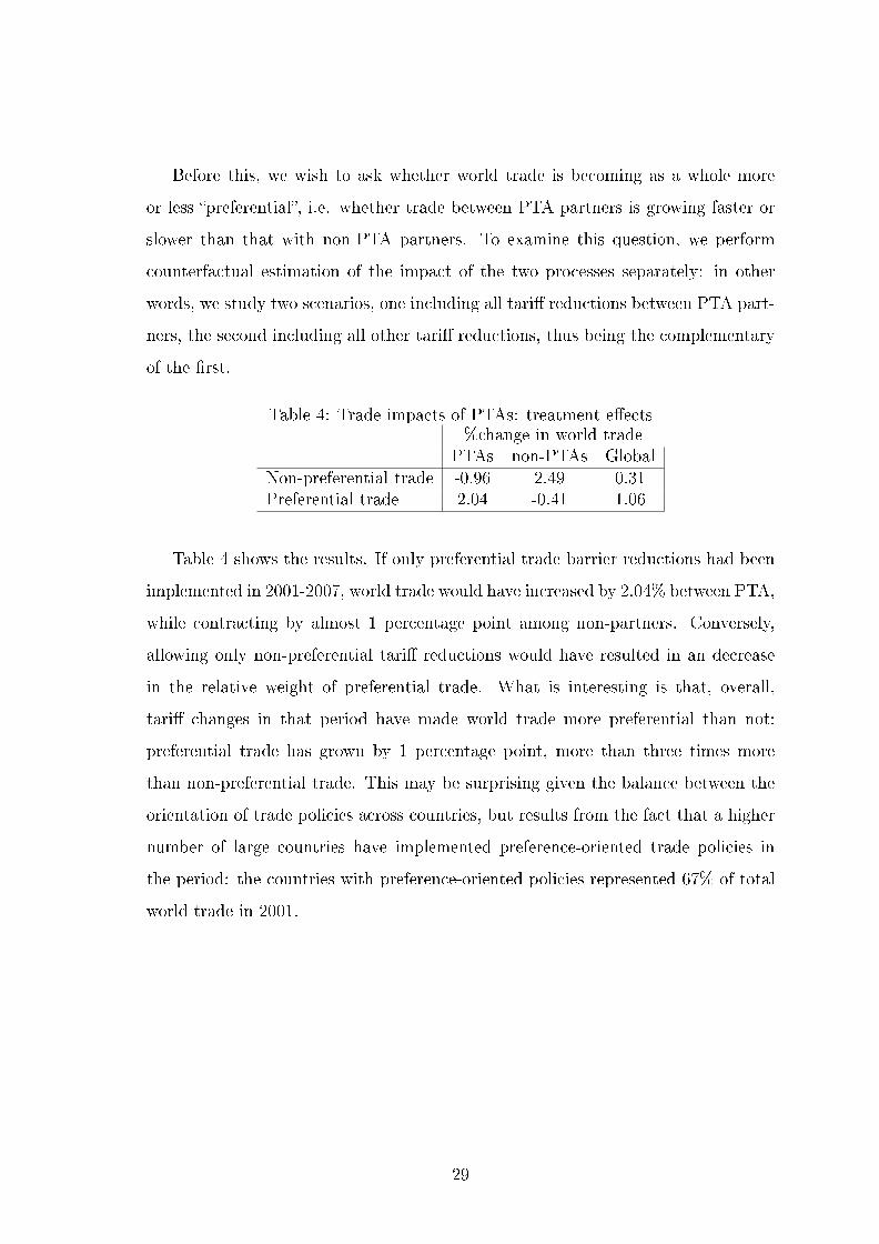
Before this, we wish to ask whether world trade is becoming as a whole more

or less �preferential�, i.e. whether trade between PTA partners is growing faster or

slower than that with non-PTA partners. To examine this question, we perform

counterfactual estimation of the impact of the two processes separately: in other

words, we study two scenarios, one including all tari� reductions between PTA part-

ners, the second including all other tari� reductions, thus being the complementary

of the �rst.

Table 4: Trade impacts of PTAs: treatment e�ects%change in world trade

PTAs non-PTAs GlobalNon-preferential trade -0.96 2.49 0.31Preferential trade 2.04 -0.41 1.06

Table 4 shows the results. If only preferential trade barrier reductions had been

implemented in 2001-2007, world trade would have increased by 2.04% between PTA,

while contracting by almost 1 percentage point among non-partners. Conversely,

allowing only non-preferential tari� reductions would have resulted in an decrease

in the relative weight of preferential trade. What is interesting is that, overall,

tari� changes in that period have made world trade more preferential than not:

preferential trade has grown by 1 percentage point, more than three times more

than non-preferential trade. This may be surprising given the balance between the

orientation of trade policies across countries, but results from the fact that a higher

number of large countries have implemented preference-oriented trade policies in

the period: the countries with preference-oriented policies represented 67% of total

world trade in 2001.

29

6 Do countries sign the most bene�cial PTAs?

We now use our model to examine the following questions: among all possible trade

agreements, how do countries choose the ones they sign? Which of the objectives

of increasing the country's real income level, or the level of its production prices, is

being best served by these choices? Finally, do they optimally choose between the

options of preferential and multilateral trade liberalization?

To answer these questions, we perform a simulation exercise in which we compute

the impacts, for each country in our sample, of all possible bilateral trade agreements

with each other country. We model these agreements as follows: the two countries

agree to reduce their tari�s to half the lowest of their two tari�s in each sector. This

is intended to capture the reciprocity that applies to most agreements.

Our approach here rests on several hypotheses. First, we assume that the content

of a PTA is su�ciently constrained by rules, so that the pro�le of tari� reductions in

any prospective agreement, conditional on initial protection levels, can be predicted

with a relative degree of accuracy. The most prominent such rule is article XXIV,

paragraph 8b of the GATT (now WTO), which requires that in a PTA �duties

and other restrictive regulations of commerce (...) are eliminated on substantially

all the trade between the constituent territories�. In practice, this means that two

countries may not sign a �partial� agreement, which would cover only a number

of selected sectors. Exceptions are , however, generally admitted to this rule, by

which a small number of product lines are being exempted from tari� dismantlement

following negotiations between parties. The number of exceptions is generally small,

both because of the GATT/WTO rule and because of con�icting interests between

negotiating governments, as each country attempts to preserve protection for its

strategic industries, while trying to gain market access for all its exporters.

Second, our simulation exercise focuses on one speci�c aspect of PTA impacts:

the terms-of-trade e�ects of preferential liberalization. Potential determinants of

trade policy also include economic factors not accounted for in our framework: in

particular specialization gains; as well as non-economic factors. For example, PTAs

may favor, or be facilitated by, political links and alliances between partners.

30

Regarding economic determinants, our hypothesis is that terms-of-trade e�ects

captured in our model constitute the most immediate e�ects of changing trade barri-

ers; while specialization or productivity gains may take longer to materialize. Assum-

ing that governments have a short-term horizon, one can thus expect terms-of-trade

e�ects to play a role in their decisions. In order to test that our results are not

driven by a correlation between these two components of PTA gains, we will per-

form robustness checks where variables capturing specialization gains are included

as controls in our regressions.

As for political determinants, we do not observe them. Our working assumption

is that such political links are not systematically correlated with our estimated price

impact, which are functions of trade costs and initial trade and protection levels.

Empirical speci�cation We model the probability of two countries signing a

PTA with the following functional form:

Pr[PTAij = 1] = F (β1.pijj + β2.P

ijj + β3.

(Yj/Pj)ML

) (18)

where F is the logistic function; Pr[PTAij = 1] is the probability of a PTA being

signed between countries i and j; p ijj and P ij

j are the predicted impacts (relative

price changes) of a PTA with country i on country j's aggregate production price

pj and consumer price index Pj, respectively. (Yj/Pj)ML) represents the predicted

impact of a multilateral reduction of tari� barriers for country i (expressed in relative

terms). This latter variable is intended to test whether the options of preferential

versus multilateral trade liberalization appear as substitutes in trade policy.

Prospective impacts p ijj , P ij

j are computed by starting from the observed level

of protection for all countries in our model in 2001, and simulating the impact of all

potential bilateral PTAs between any pair countries, while maintaining status quo

on all other trade barriers. PTAs are modeled as described at the beginning of this

section. (Yj/Pj)ML) is computed as the result of a multilateral opening of country

j's trade, modeled as a uniform cut of 50% on all tari�s barriers. The dependent

variable is a binary indicator of a PTA being signed between two countries after

2001.

31

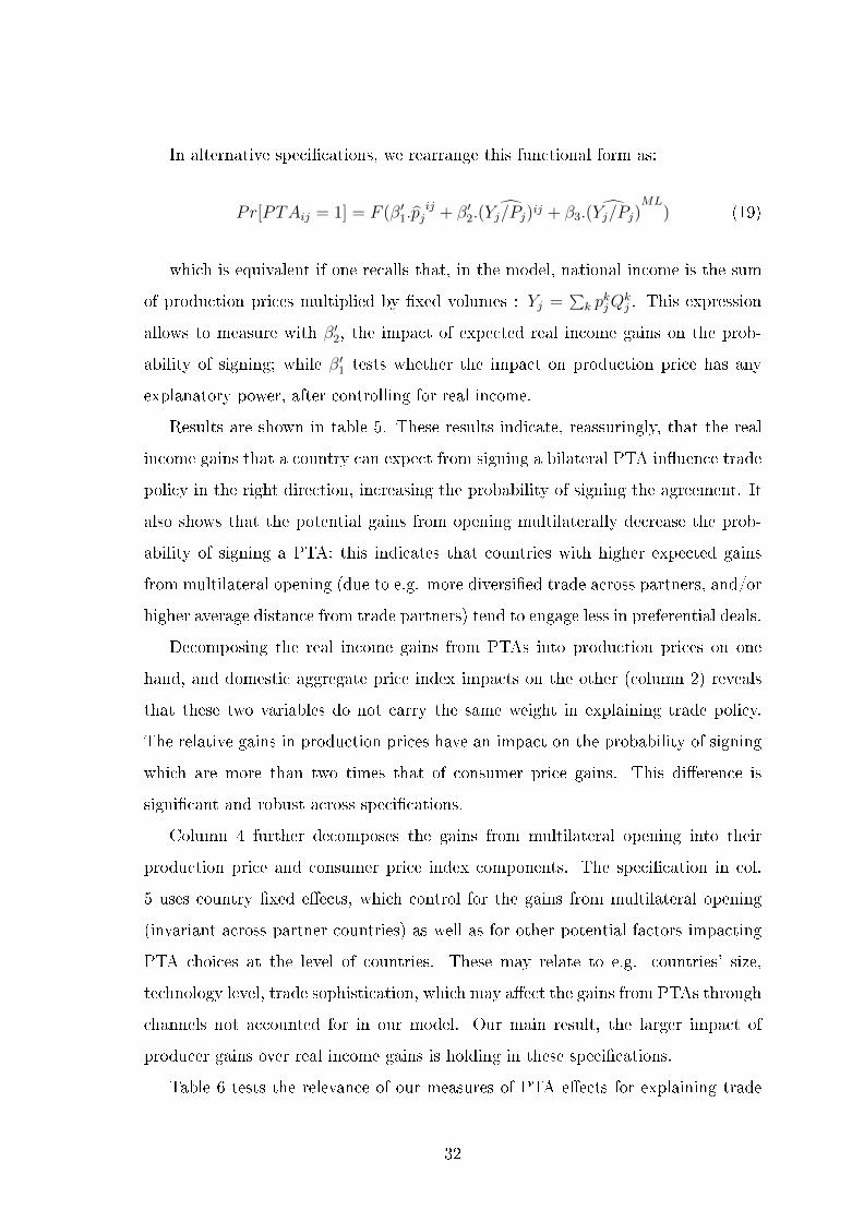
In alternative speci�cations, we rearrange this functional form as:

Pr[PTAij = 1] = F (β′1.pijj + β′2.

(Yj/Pj)ij + β3.(Yj/Pj)

ML) (19)

which is equivalent if one recalls that, in the model, national income is the sum

of production prices multiplied by �xed volumes : Yj =∑k p

kjQ

kj . This expression

allows to measure with β′2, the impact of expected real income gains on the prob-

ability of signing; while β′1 tests whether the impact on production price has any

explanatory power, after controlling for real income.

Results are shown in table 5. These results indicate, reassuringly, that the real

income gains that a country can expect from signing a bilateral PTA in�uence trade

policy in the right direction, increasing the probability of signing the agreement. It

also shows that the potential gains from opening multilaterally decrease the prob-

ability of signing a PTA: this indicates that countries with higher expected gains

from multilateral opening (due to e.g. more diversi�ed trade across partners, and/or

higher average distance from trade partners) tend to engage less in preferential deals.

Decomposing the real income gains from PTAs into production prices on one

hand, and domestic aggregate price index impacts on the other (column 2) reveals

that these two variables do not carry the same weight in explaining trade policy.

The relative gains in production prices have an impact on the probability of signing

which are more than two times that of consumer price gains. This di�erence is

signi�cant and robust across speci�cations.

Column 4 further decomposes the gains from multilateral opening into their

production price and consumer price index components. The speci�cation in col.

5 uses country �xed e�ects, which control for the gains from multilateral opening

(invariant across partner countries) as well as for other potential factors impacting

PTA choices at the level of countries. These may relate to e.g. countries' size,

technology level, trade sophistication, which may a�ect the gains from PTAs through

channels not accounted for in our model. Our main result, the larger impact of

producer gains over real income gains is holding in these speci�cations.

Table 6 tests the relevance of our measures of PTA e�ects for explaining trade

32

policy. In a seminal paper, Baier and Bergstrand (2004) develop a model of trade

which they use to derive a list of determinants of the potential gains from a PTA;

they then show that this list allows to correcly predict a number of the agreements

which were actually signed. Their model includes several dimensions of the gains

from PTAs, including specialization gains. By contrast, our approach is restricted to

more speci�c gains from PTAs, namely terms-of-trade gains; but we measure these

gains structurally. To test if our model adds some elements to ther understanding

of countries' trade policy, we run in table 6 regressions including the two lists of

variables.

Natural is a dummy for two countries being on the same continent. It captures

the gains from singing PTAs with so-called `natural partners', yielding higher gains

because of the more intense trade relations. Remote is a proxy measure of the

distance of two partners from the rest of the world countries, distance which increases

the PTA gains as diversion e�ects are reduced. Finally, drgdp is a measure of the

gap in income levels between two countries and captures the similarity between two

economies.

Results show that although these variables have some power to explain PTAs,

they do not exhaust the determinants of countries' trade policy; in particular, our

measures of PTA price impacts remain signi�cant.

Finally, table 7 introduces a measure of the losses faced by a country if one

of its trade partners engages with a PTA with a third country. Baldwin (1993)

has proposed that contagion or �domino e�ects� may explain the �proliferation�

of preferential agreements, as trade diversion from PTAs creates an incentive for

non-members to join existing agreements, or to form new ones. Here we test this

hypothesis by using a proxy measure of the loss to third countries: for each pair (A,B)

of countries, we compute the real income changes for A in scenarios where B signs

an agreement with a third country. These changes are negative, due to diversion.

We take the maximum loss incurred by A across all potential PTAs signed by B, and

use this as a proxy measure of the �diversion threat�. This measure is introduced

in our speci�cation in column 1, and decomposed in column 2 into the production

and price index components. Results indicate that the magnitude of this potential

33

loss relates to the probability of signing an agreement, which tends to con�rm the

contagion hypothesis. Column 3 we build the PTA �net impacts� on prices, de�ned

as the impact of signing an agreement, minus the loss in the case no agreement is

signed and the partner country engages in another PTA. The larger imp

Table 5: Determinants of PTA signing(1) (2) (3) (4) (5)

Pr[PTA = 1]Real income impact of bilateral PTA 0.63a 0.63a 0.81a

(0.10) (0.10) (0.14)

PTA impact on production prices 1.42a 0.79c 1.44a 1.32b

(0.48) (0.47) (0.49) (0.52)

PTA impact on domestic price index -0.63a -0.63a

(0.10) (0.10)

Real income impact of multilateral opening -0.25a -0.24a -0.24a

(0.06) (0.06) (0.06)

ML opening: prod. prices -0.33(0.26)

ML opening: domestic price index 0.24a

(0.06)Country �xed-e�ects yesObservations 1722 1722 1722 1722 1148Pseudo R2 0.053 0.056 0.056 0.056 0.136Standard errors in parentheses.c p<0.1, b p<0.05, a p<0.01

Logit regression on the probability of a PTA being signed between two countries in or after 2001.Impact of each PTA on production f.o.b. prices and on the domestic price index (CES price index)are used in % variation. They are computed at sector level, then aggregated consistently with themodel structure. See text for the de�nition of PTAs in the simulation exercise.

34

Table 6: Determinants of PTAs: robustness checks(1) (2) (3)

Pr[PTA = 1]PTA impact: production prices 1.21b 1.21b 1.17b

(0.48) (0.48) (0.48)

PTA impact: domestic price index -0.64a -0.64a -0.57a

(0.10) (0.10) (0.11)

Real income impact of multilateral opening -0.24a -0.25a -0.24a

(0.06) (0.06) (0.06)

Natural 0.49b 0.50b 0.56a

(0.21) (0.21) (0.22)

Remote -0.15 -0.15(0.54) (0.54)

Drgdp 0.09(0.06)

Observations 1722 1722 1722Pseudo R2 0.062 0.062 0.065Standard errors in parentheses.c p<0.1, b p<0.05, a p<0.01

Regressions in this table add to the former speci�cation used in table 5 the determinants of PTAsas identi�ed in Baier and Bergstrand (2004). Natural is 1 if the two countries are on the samecontinent. Remote is the average distance of the two partners to other countries outside the pair.Drgdp is the absolute value of the di�erence of the log of real GDPs of the two partners.

35

Table 7: Determinants of PTAs: diversion e�ects(1) (2) (3)

Pr[PTA = 1]Real income impact of bilateral PTA 0.47a 0.49a

(0.12) (0.13)

Diversion: real income impact -6.82a

(2.49)

Diversion: production prices -4.33a

(1.31)

Diversion: domestic prices 0.14(3.45)

Production prices: net impact 1.36a

(0.39)

Domestic prices: net impact -0.59a

(0.10)

Real income impact of multilateral opening -0.24a -0.22a -0.23a

(0.06) (0.06) (0.06)Observations 1722 1722 1722Pseudo R2 0.060 0.065 0.060Standard errors in parentheses.c p<0.1, b p<0.05, a p<0.01

Regressions in this table add estimates of the potential losses by diversion faced byone country if the partner country implements another PTA with a third country.These impacts are decomposed into e�ects on production prices, domestic CES priceindex and overall real income impact. �Net impacts� are the di�erence between theimpact of signing a PTA, and the impact if the partner country signs with a thirdcountry.

36

7 Conclusion

What determines trade policy has been a recurrent question in the literature. In

this paper we have proposed an original approach to it, based on observing trade

policies in the data and looking at the implied trade and income e�ects. First, we

looked at all tari� changes implemented by world countries during 2001-2007, and

used a general equilibrium model to compute the implied impacts on trade patterns,

and on country real GDP and welfare levels. Although simple, our model essentially

captures terms-of-trade e�ects of preferential and multilateral trade liberalization,

thus allowing to quantify trade creation and diversion e�ects. This exercise reveals

that both preferential and multilateral liberalizations are being implemented con-

currently by most world countries; overall, about half the countries in our sample

have been running a trade policy more multilateral than preferential, thus reducing

distorsions in their tari� structure. Next, we found tthe choice of trade policy to be

strongly related to both producer and consumer interests, with the former having a

weight about two times larger. In contrast to previous estimates in the literature,

this result shoows the presence of important distorsions in the setting of trade pol-

icy. It suggests that the excessive weight put on market access gains leads countries

to exhibit a bias in favor of preferential trade liberalization, despite larger expected

gains from multilateral opening.

37

References

Anderson, J. and E. v. Wincoop (2003). Gravity with gravitas: A solution to the

border puzzle. American Economic Review 93 (1), 170â�192.

Anderson, J. and Y. V. Yotov (2010a). The changing incidence of geography. Amer-

ican Economic Review 100 (3), 2157â�86.

Anderson, J. and Y. V. Yotov (2011). Terms of trade and global e�ciency e�ects of

free trade agreements, 1990-2002. NBER Working Papers # 17003 .

Anderson, J. E. and Y. V. Yotov (2010b). Specialization: Pro- and anti-globalizing,

1990-2002. NBER Working Paper 16301, National Bureau of Economic Research,

Inc.

Anderson, J. E. and Y. V. Yotov (2012). Gold standard gravity. NBER Working

Paper 17835, National Bureau of Economic Research, Inc.

Arkolakis, C., A. Costinot, and A. Rodriguez-Clare (2012). New trade models, same

old gains? American Economic Review 102 (1), 94�130.

Baier, S. and J. Bergstrand (2007). Do free trade agreements actually increase

members' international trade? Journal of International Economics 71 (1), 72â�95.

Baier, S. and J. Bergstrand (2009). Bonus vetus OLS: a simple method for ap-

proximating international trade-cost e�ects using the gravity equation. Journal

of International Economics 77 (1), 77�85.

Baier, S. L. and J. H. Bergstrand (2004). Economic determinants of free trade

agreements. Journal of International Economics 64 (1), 29�63.

Baldwin, R. (1993). A domino theory of regionalism. NBER working paper # 4465 .

Eaton, J. and S. Kortum (2002). Technology, geography and trade. Economet-

rica 70 (5), 1741â�1779.

38

Egger, P., M. Larch, K. E. Staub, and R. Winkelmann (2011). The trade e�ects

of endogenous preferential trade agreements. American Economic Journal: Eco-

nomic Policy 3 (3), 113â�43.

Goldberg, P. K. and G. Maggi (1999, December). Protection for sale: An empirical

investigation. The American Economic Review 89 (5), 1135�1155. ArticleType:

research-article / Full publication date: Dec., 1999 / Copyright  c© 1999 Ameri-

can Economic Association.

Grossman, G. (1994). "Import Competition from Developed and Developing

Countries". Review of Economics and Statistics 64, 271â�281.

Grossman, G. M. and E. Helpman (1995). The politics of free-trade agreements.

American Economic Review 85 (4), 667�90.

Imbs, J. and I. Mejean (2009). Elasticity optimism. CEPR Discussion Paper 7177,

C.E.P.R. Discussion Papers.

Krugman, P. (1979). "Increasing returns, monop�listic competition and interna-

tional trade". Journal of International Economics 9 (4), 469â�479.

Melitz, M. J. (2003, November). The Impact of Trade on Intra-Industry Realloca-

tions and Aggregate Industry Productivity. Econometrica 71 (6), 1695�1725.

Neary, J. P. and M. Mrazova (2013, December). Not so demanding: Preference struc-

ture, �rm behavior, and welfare. Economics Series Working Paper 691, University

of Oxford, Department of Economics.

Rauch, J. E. (1999). Networks versus markets in international trade. Journal of

International Economics 48 (1), 7�35.

WTO (2011). World Trade Report 2011. The World Trade Organization, Geneva.

39

Appendices

A Estimation of sector elasticities

40

Table 8: Sector elasticities estimatesSectors Coe�. std. Obs. Sectors Coe�. std. Obs.ISIC error ISIC error

(1) (2) (3) (1) (2) (3)101 -3.75 2.88 1602 251 -5.97 0.55 7833102 -4.1 2.52 1250 252 -7.98 0.58 8390103 -4.1 2.52 1250 261 -8.06 0.63 6871111 -1.24 0.22 8025 269 -3.22 0.77 7651112 -0.33 0.29 5584 271 -4.19 0.78 7634113 -1.95 0.26 7839 272 -7.15 0.93 7097121 -0.86 0.48 2056 281 -4.63 0.73 5981122 -0.21 0.29 4697 289 -4.19 0.58 8885131 -10.8 2.41 3924 291 -6.31 0.72 9006132 -10.8 2.41 3924 292 -5.46 1.26 8967141 -5.96 0.99 4321 293 -5.14 0.59 6367142 -4.96 1.23 5356 300 -6.8 1.44 7819151 -1.93 0.24 8811 311 -6.48 0.99 7236152 -1.34 0.31 4312 312 -5.3 0.83 7147153 -1.03 0.17 5942 313 -7.7 0.83 5818154 -0.88 0.21 8059 314 -4.5 0.75 5359155 -0.34 0.11 5826 315 -4.02 0.59 6313160 -0.66 0.21 3794 319 -4.43 0.84 6734171 -2.76 0.58 7772 321 -9.44 1.3 6341172 -3.66 0.51 8150 322 -0.76 0.62 6548173 -2.72 0.59 7144 323 -3 0.65 6968181 -2.8 0.38 8400 331 -5.71 1 8203182 -1.16 0.87 2448 332 -2.09 0.82 5801191 -4.98 0.57 6929 333 -2.53 0.83 4508192 -3.6 0.48 6390 341 -3.96 0.47 6633200 -1.58 0.5 5542 342 -2.84 0.63 4572201 -4.13 1.1 5112 343 -6.94 0.67 7262202 -3.62 0.56 7099 351 -4.1 1.4 3596210 -7 0.69 7445 352 -12.97 2.01 2571221 -6.71 0.74 6998 353 -7.99 1.66 4541222 -4.48 0.59 5799 359 -2.56 0.56 5032231 -4.75 4.03 1164 361 -5.07 0.49 7348232 -3.69 0.99 6004 369 -0.79 0.21 8759233 -5.19 2.59 1713 372 -2.38 1.23 1836241 -8.77 0.87 9059 500 -1.2 0.6 4370242 -1.31 0.43 9535 742 -6.63 3.27 1366243 -4.47 1.05 4772 749 -9.91 1.57 1763

921 -3.27 0.76 4362Notes: Estimation of sector-level CES demand elasticities based on equa-tion (2). Heteroscedasticity-robust standard errors are reported in paren-theses. Estimations use importer-year and exporter-year �xed-e�ects. Thetable reports coe�cients obtained on the tari� variable, which correspondsto the factor 1− σ in the model. R2 vary in the range of 0.6-0.86.

41