uncertainty budgeting in system design...y standard deviation of qoi y;b budget on the standard...

Sensitivity Analysis Methods for Uncertainty

Budgeting in System Design

Max M. J. Opgenoord∗ and Karen E. Willcox†

Massachusetts Institute of Technology, Cambridge, MA, 02139

Quantification and management of uncertainty are critical in the design of engineer-ing systems, especially in the early stages of conceptual design. This paper presents anapproach to defining budgets on the acceptable levels of uncertainty in design quantitiesof interest, such as the allowable risk in not meeting a critical design constraint and theallowable deviation in a system performance metric. A sensitivity-based method analyzesthe effects of design decisions on satisfying those budgets, and a multi-objective optimiza-tion formulation permits the designer to explore the tradespace of uncertainty reductionactivities while also accounting for a cost budget. For models that are computationallycostly to evaluate, a surrogate modeling approach based on high dimensional model repre-sentation (HDMR) achieves efficient computation of the sensitivities. An example problemin aircraft conceptual design illustrates the approach.

Nomenclature

C Cost of changing the distributions ofthe input variables

CL Cruise aircraft lift coefficientCb Budget on the cost of changes in the

input distributionsF Objective function for optimization

problemG Nonlinear constraint for optimization

problemKn Input space mapped to the unit hy-

percubeMTOW Maximum Takeoff WeightN Number of samplesOPR Overall pressure ratioP Risk of QoI exceeding rP0 Risk of QoI exceeding r for nominal

input variable distributionsPb Budget on the risk of the QoIP ′ Updated risk for changes in the distri-

butions of the input variablesSi, Sij , . . . Sensitivity indicesTmetal Turbine metal temperature(Tt4)CR Turbine inlet total temperature for

cruiseVi, Vij , . . . Variance of component functions of

HDMRf Probability density function

fY (r) Value of the probability density func-tion of y at y = r

g Engineering system representation,prescribing the relation between theinput variables and the QoI

g0, gi, gij , . . . Component functions of HDMR sur-rogate

n Number of input variablesp Risk of QoI y exceeding the value rsfus Maximum allowable fuselage shell

bending stressswt Maximum allowable wing and tail spar

cap stressx, xi, xj Input variablesy Quantity of interest (QoI)

Symbols

α, β, γ Weighting parameters for the objec-tive function

αir Weighting coefficient for first-ordercomponent functions

βijpq Weighting coefficient for second-ordercomponent functions

µ Vector containing the mean of each in-put variable

µY Mean of QoIσ Vector containing the standard devia-

tion of each input variable

∗Graduate student, Department of Aeronautics and Astronautics, [email protected], Student Member AIAA†Professor of Aeronautics and Astronautics, [email protected], Associate Fellow AIAA

1 of 25

American Institute of Aeronautics and Astronautics

σY Standard deviation of QoIσY,b Budget on the standard deviation of

the QoI

ϕi Basis functionsξ Running parameter for basis functions

I. Introduction

This paper presents a sensitivity-based methodology to support decision-making in the design of multi-disciplinary engineering systems, with a focus on the challenge of quantifying and managing uncertainty.

We consider the early stages of the design phase, where quantification of uncertainty permits designers toidentify critical areas of design risk and to allocate resources accordingly.Uncertainties abound in engineeringdesign and decision: technical uncertainties due to novel configurations and new technologies, programmaticuncertainties in cost and schedule, design requirements and/or operating conditions that may evolve overtime, and uncertainties introduced due to the use of simplified models. These uncertainties pose a seriousrisk to the critical decisions made in engineering design, especially when considering novel systems for whichexperience and historical data are lacking. Despite a growing recognition of the importance of accountingfor uncertainties, systematic methods to quantify and manage uncertainty remain a significant challenge,especially for systems that comprise many interacting subcomponents and/or disciplines.

Past work has addressed the challenge of forward propagation of uncertainty: Given uncertain parametersand uncertain system inputs, what is the corresponding uncertainty in the outcome? Uncertain outcomesare typically characterized by uncertainty associated with the design quantities of interest (QoI).1,2, 3 Theliterature categorizes uncertainty as epistemic, owing to insufficient or imperfect knowledge, or aleatory,which arises from natural randomness and is therefore irreducible.2,4, 5, 6 Other work has distinguished amongseveral types of uncertainty, including the many sources associated with the use of computer-based simulationmodels in system design.7 In this paper, we use probabilistic models to represent uncertainty in designparameters and QoI.2,8, 9 Other ways of characterizing uncertainty include using a probability box to capturethe imprecision in the available uncertainty information.10 Regardless of the method chosen to representuncertainty, forward propagation of uncertainty typically involves repeated model evaluations to conduct theneeded sampling; thus, a great deal of recent work has focused on methods to reduce computational expense,including the use of less-expensive surrogate models to approximate system response.11,12,13,14,15,16

Sensitivity analysis targets the inverse question: What are the uncertain parameters and inputs thatcontribute the most to output variability, and how would reducing uncertainty in these parameters lead toreduction in output uncertainty? In the context of engineering system design, sensitivity analysis permits bet-ter understanding of the effects of uncertainty in order to make well-informed decisions aimed at uncertaintyreduction.8,17 Existing sensitivity analysis approaches typically use variance as a measure of uncertainty.The process of apportioning output variance across model factors in a global sensitivity analysis can be car-ried out by both a Fourier Amplitude Sensitivity Test (FAST) method, and the Sobol’ method.18,19,20,21,22

The FAST method is based on Fourier transforms, while the Sobol’ method utilizes Monte Carlo simulation.In addition to variance-based sensitivity analysis, work has also been done in the development of methodsfor global and regional sensitivity analysis using information entropy as a measure of uncertainty. One suchmethod uses the Kullback-Leibler (K-L) divergence, or relative entropy, to quantify the distance between twoprobability distributions.23 These distributions correspond to estimates of the QoI before and after somemodel parameter has been fixed at a particular value (e.g., its mean value). The K-L divergence between thetwo distributions then serves to quantify the impact of the factor that has been fixed: the larger the valueof the K-L divergence, the more substantial the contribution of that parameter to uncertainty in the QoI.

In addressing design under uncertainty, robustness—which according to Knoll and Vogel is “the propertyof systems that enables them to survive unforeseen or unusual circumstances”24—and reliability—which de-scribes a system’s “probability of success in satisfying some performance criterion”1—are typically treatedseparately. The origins of robust design stem back to the pioneering work of Taguchi, with the aim of re-ducing the sensitivity of products and processes to various noise factors, such as manufacturing variability,environmental conditions, and degradation over time.25,26,27 In Ref. 28, an integrated framework for opti-mization under uncertainty is developed that accounts for both design objective robustness and probabilisticdesign constraints.

This paper develops a broadly applicable sensitivity-based methodology that, given a model of the sourcesof uncertainty, provides systematic guidance to a decision-maker in identifying and selecting uncertaintyreduction options and design choices. Our goal is to allocate the resources of cost, schedule and risk,

2 of 25


while also identifying opportunities to tailor the design so as to minimize uncertainty in key areas whileretaining flexibility in others. Underlying our proposed approach is the view that uncertainty is a currency:a designer can tolerate a particular level of uncertainty, typically characterized by specified acceptable levels(i.e., budgets) of risk, reliability and/or robustness. The key challenge then becomes how to “spend” theuncertainty—where to focus uncertainty reduction efforts so as not to waste valuable resources reducinguncertainty in parameters that contribute little to output uncertainty, but instead to target the most sensitiveparameters and manage resources in a systematic way. This modeling of the design process is consistentwith decomposition-based formulations of the design problem, such as analytical target cascading (ATC),where the system is modeled using hierarchical levels and design targets are cascaded from upper levelsto lower levels.29,30,31 Similar ideas are explored in Chen et al., who propose a method that reverses thecomputational flow in a design code.32 That work builds on the univariate reduced quadrature method ofPadulo et al.,33 which represents the QoI standard deviation as a function of the first four moments of aunivariate input distribution.

Our work builds on the mathematical framework of Ref. 34, which views the system design problem asa stochastic estimation process as shown in Figure 1. The term “stochastic estimation process” is used toconvey the idea that the design process can be modeled as an iterative process of resolving uncertainty. Thatis, at any point in time the design is represented through a set of state variables, each with an associateduncertainty. Design effort results in the generation of new information (“measurements”), which can be usedto update the uncertain design state. This process continues until the uncertainty is resolved to acceptablelevels. In this paper, we advance that work by formalizing the idea of uncertainty budgeting. In particular,we formulate and solve a multi-objective optimization problem that seeks optimal strategies to manage theuncertainty and design risk. A second contribution of the paper is to introduce a tailored surrogate modelingapproach that permits analysis of complex system models. The remainder of the paper is organized asfollows. Section II provides a description of the problem formulation and background on the sensitivityanalysis methods. Section III describes the uncertainty budgeting methodology and formulates the resourceallocation optimization problem. Section IV presents a surrogate modeling approach that can be used toreduce the computational expense of solving the uncertainty budgeting optimization problem. Section Vdemonstrates the approach by presenting illustrative examples in conceptual aircraft design focusing onpropulsion uncertainty and uncertainty coming from multiple disciplines. Finally, Section VI concludes thepaper.

II. Problem Formulation and Background

This section defines the problem formulation in Section II.A, and introduces background on high dimen-sional model representation (HDMR) and analysis of variance (ANOVA) in Section II.B.

II.A. Problem formulation

In the initial stages of designing a complex system, the key inputs for that design are still uncertain. In aircraftdesign, for instance, engine technology has a major influence on the design, but may not be fixed at the startof the design phase because of possible future advances.36 However, the designers still have requirements forthe system, and the risk of not meeting those requirements must be quantified and mitigated. Furthermore,key QoI describing the performance and cost of the design are also uncertain during early design stages. Thisuncertainty must be managed to acceptable levels as the design process evolves. In this work, we formalizethe view that uncertainty is a currency: a designer can tolerate a particular level of uncertainty; the decisionthen becomes how to “spend” the uncertainty. To formulate this mathematically, we define cost budgetsand uncertainty budgets. The uncertainty budget allocates quantitative limits on the acceptable risk in notmeeting design requirements and on the acceptable variability in the design QoI (i.e., it specifies the desiredreliability and robustness of the design). The cost budget allocates quantitative limits on the resources thatcan be expended on uncertainty reduction (e.g., money, time, computational resources).

We consider a general system, represented as

y = g(x),

where y is the system QoI, x are the system input variables, and g is the mapping from input x to QoI y.Throughout this paper this system mapping is considered as a general black box—it could be, for example,

3 of 25


Set TargetsDefine Input

VariableDistributions

GenerateDesigns

EvaluateQuantitiesof Interest

QuantifyUncertainty

PerformSensitivityAnalysis

Requirements,Constraints

X1

f(X1)

X2

f(X2) Y = g (x)

Y

f(Y )

DesignFeedback

UncertaintyFeedback

ResourceAllocation

Robustness, Reliability, Cost

Variance, Risk

QOI

Figure 1. Modeling the system design as a stochastic estimation process with feedback. Figure adapted fromRef. 35.

a computational model or an experiment; however, it is assumed that there is freedom in choosing the inputvalues (i.e., the function g(x) can be evaluated for input x). In the following we develop the methodologyfor a single scalar QoI, although the approach is straightforward to apply to the case of multiple QoI.

We represent the uncertainty in the input variables probabilistically, that is, we consider x to be arandom variable and we describe each component of x using a probability density function (PDF). ThePDFs for each input variable are specified by the designer and could be determined from historical dataor expert opinion. In current engineering practices, such PDFs are typically not readily available and thisis often put forward as a barrier against using probabilistic methods. In some cases, sufficient informationand data will be available to infer a reasonable PDF—for example, when considering uncertainty associatedwith an advanced technology, one can often draw on experimental results that provide informed choices ofparameter ranges and probable values. However, in many cases, engineering judgement will be required todefine suitable PDFs for the input parameters. While this is certainly an important challenge that must beaddressed, current design practices simply ignore uncertainty, or they account coarsely for it by using safetyfactors on the resulting design choices.a

The uncertainty in inputs induces uncertainty in the output QoI; thus, y is also modeled as a randomvariable. The PDF of y is estimated using Monte Carlo simulation to propagate uncertainty through thesystem. We then set budgets on allowable cost and uncertainty. In this work we consider a budget onthe allowable standard deviation of the QoI, a budget on the allowable probability of not meeting designrequirements, and a budget on the allowable cost of the changes in the input variables. Every design changehas an associated cost—whether it be a cost associated with a change in the mean values of the inputvariables, or a cost associated with a reduction in input uncertainty. The problem therefore becomes aconstrained optimization problem to find the best resource allocation strategy that satisfies both cost anduncertainty budgets. This is described mathematically in Section III. Our approach to formulating andsolving this problem uses a global sensitivity analysis (GSA), built on the theory of high dimensional modelrepresentation (HDMR). The next subsection gives background on HDMR and GSA.

aAs Richard Feynman eloquently puts it: “I can live with doubt and uncertainty and not knowing. I think it is much moreinteresting to live not knowing than to have answers that might be wrong. If we will only allow that, as we progress, we remainunsure, we will leave opportunities for alternatives.”

4 of 25


II.B. High Dimensional Model Representation (HDMR) and Global Sensitivity Analysis(GSA)

HDMR is an analysis tool used in representing the relationship between inputs and outputs in a generalmodel.37,38,39 In this method, the function g(x) is expanded into independent component subfunctions interms of the input variables,

g (x) = g0 +

n∑i=1

gi (xi) +∑

1≤i<j≤n

gij (xi, xj) + . . .

+∑

1≤i1<...<il≤n

gi1i2...il (xi1 , xi2 , . . . , xil) + . . .+ g12...n (x1, x2, . . . , xn) . (1)

Here, g0 represents the mean response of g (x) over the input space, while the component subfunction gi (xi)captures the contribution of the ith input variable alone. We use the notation xi to denote the ith inputvariable and we consider the case of n input variables, x = [x1, . . . , xn]>. The component subfunctiongij (xi, xj) represents the correlated contribution of the ith and jth input variable to g (x), and so on.

The decomposition as written in Eq. (1) is not unique.4 It can however be uniquely defined by imposingthe vanishing condition,40,41,42 which states that the integral of an HDMR component function with respectto any of its own variables is zero:43∫ 1

0

fs (xs) gi1i2...ik (xi1 , xi2 , . . . , xik) dxs = 0 ∀s ∈ {i1, i2, . . . , ik} , (2)

where fs (xs) is the probability density function of the sth input variable. Note that for ease of presentationand without loss of generality, the variables xi have been rescaled by a suitable transformation such that0 ≤ xi ≤ 1 ∀i. The HDMR representation with constraint (2) is called the ANOVA-HDMR; as described inthe following, the resulting functional decomposition of g(x) provides a quantitative basis on which to assesshow the various inputs contribute to QoI uncertainty.44,45

Because of the orthogonality constraints in Eq. (2), the variance of the QoI can be expressed as

V (y) =∑i

Vi +∑

1≤i<j≤n

Vij + . . .+ V12...n, (3)

where Vi is the portion of the QoI variance associated with the subfunction gi,

Vi = V (gi (xi)) = V [E (y|xi)] , (4)

and Vij is the portion of the QoI variance associated with the subfunction gij ,

Vij = V (gij (xi, xj)) = V [E (y|xi, xj)]− V [E (y|xi)]− V [E (y|xj)] . (5)

Similar expressions can be built up for Vijk and further. Dividing by the total variance, the decompositionof sensitivity indices is obtained, ∑

i

Si +∑

1≤i<j≤n

Sij + . . .+ S12...n = 1, (6)

where Si = Vi/V , Sij = Vij/V , and so on for the higher-order terms. The main effect sensitivity index Sirepresents the normalized expected reduction in total variance if the variance of the ith input variable werereduced to zero. Computing these sensitivity indices is termed a global sensitivity analysis (GSA).44

III. Uncertainty Budgets in System Design

Figure 2 illustrates our overall uncertainty quantification method. Section III.A describes the initial prob-lem setup. Section III.B formulates a multi-objective optimization problem to solve the resource allocationproblem and Section III.C discusses the solution to the optimization problem.

5 of 25


Initial problem setupUncertainty

reduction costs

Initial distributions

Uncertainty andcost budgets on QoIBaseline Global Sensitivity

Analysis (GSA)

Choose relevantinput parameters

Resource allocationoptimization

Optimizer

Evaluate standarddeviation, cost and

risk for updateddistribution

Evaluate objectivefunction and checkif budgets are met

Results visualization& assessment

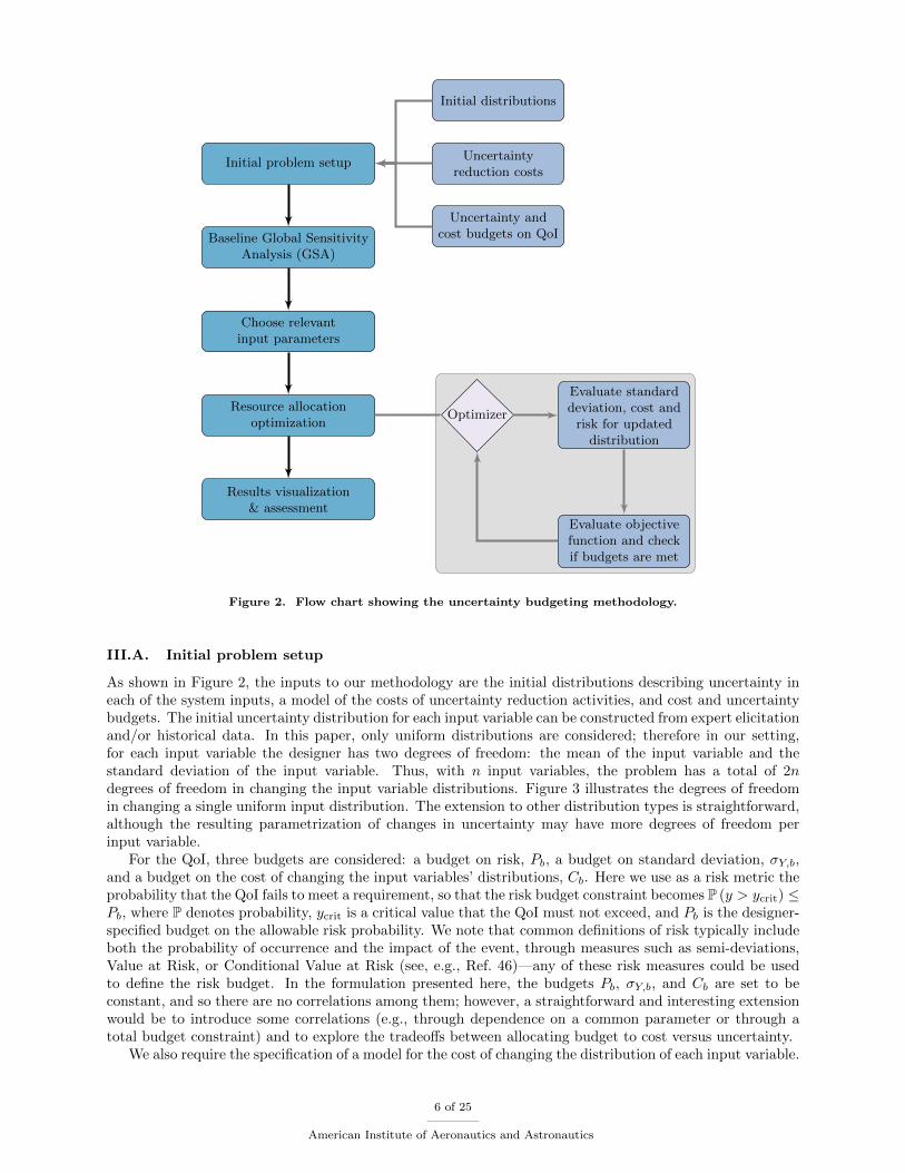
Figure 2. Flow chart showing the uncertainty budgeting methodology.

III.A. Initial problem setup

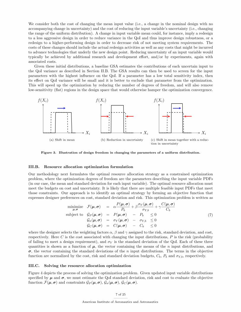
As shown in Figure 2, the inputs to our methodology are the initial distributions describing uncertainty ineach of the system inputs, a model of the costs of uncertainty reduction activities, and cost and uncertaintybudgets. The initial uncertainty distribution for each input variable can be constructed from expert elicitationand/or historical data. In this paper, only uniform distributions are considered; therefore in our setting,for each input variable the designer has two degrees of freedom: the mean of the input variable and thestandard deviation of the input variable. Thus, with n input variables, the problem has a total of 2ndegrees of freedom in changing the input variable distributions. Figure 3 illustrates the degrees of freedomin changing a single uniform input distribution. The extension to other distribution types is straightforward,although the resulting parametrization of changes in uncertainty may have more degrees of freedom perinput variable.

For the QoI, three budgets are considered: a budget on risk, Pb, a budget on standard deviation, σY,b,and a budget on the cost of changing the input variables’ distributions, Cb. Here we use as a risk metric theprobability that the QoI fails to meet a requirement, so that the risk budget constraint becomes P (y > ycrit) ≤Pb, where P denotes probability, ycrit is a critical value that the QoI must not exceed, and Pb is the designer-specified budget on the allowable risk probability. We note that common definitions of risk typically includeboth the probability of occurrence and the impact of the event, through measures such as semi-deviations,Value at Risk, or Conditional Value at Risk (see, e.g., Ref. 46)—any of these risk measures could be usedto define the risk budget. In the formulation presented here, the budgets Pb, σY,b, and Cb are set to beconstant, and so there are no correlations among them; however, a straightforward and interesting extensionwould be to introduce some correlations (e.g., through dependence on a common parameter or through atotal budget constraint) and to explore the tradeoffs between allocating budget to cost versus uncertainty.

We also require the specification of a model for the cost of changing the distribution of each input variable.

6 of 25


We consider both the cost of changing the mean input value (i.e., a change in the nominal design with noaccompanying change in uncertainty) and the cost of reducing the input variable’s uncertainty (i.e., changingthe range of the uniform distribution). A change in input variable mean could, for instance, imply a redesignto a less aggressive design in order to reduce variance in the QoI and thus improve design robustness, or aredesign to a higher-performing design in order to decrease risk of not meeting system requirements. Thecosts of these changes should include the actual redesign activities as well as any costs that might be incurredto advance technologies that underly the new design point. Reducing uncertainty of an input variable wouldtypically be achieved by additional research and development effort, and/or by experiments, again withassociated costs.

Given these initial distributions, a baseline GSA estimates the contributions of each uncertain input tothe QoI variance as described in Section II.B. The GSA results can then be used to screen for the inputparameters with the highest influence on the QoI. If a parameter has a low total sensitivity index, thenits effect on QoI variance will be small and it is better to exclude that parameter from the optimization.This will speed up the optimization by reducing the number of degrees of freedom, and will also removelow-sensitivity (flat) regions in the design space that would otherwise hamper the optimization convergence.

Xi

f(Xi)

(a) Shift in mean

Xi

f(Xi)

(b) Reduction in uncertainty

Xi

f(Xi)

(c) Shift in mean together with a reduc-tion in uncertainty

Figure 3. Illustration of design freedom in changing the parameters of a uniform distribution.

III.B. Resource allocation optimization formulation

Our methodology next formulates the optimal resource allocation strategy as a constrained optimizationproblem, where the optimization degrees of freedom are the parameters describing the input variable PDFs(in our case, the mean and standard deviation for each input variable). The optimal resource allocation mustmeet the budgets on cost and uncertainty. It is likely that there are multiple feasible input PDFs that meetthose constraints. Our approach is to identify an optimal strategy by forming an objective function thatexpresses designer preferences on cost, standard deviation and risk. This optimization problem is written as

minimizeµ,σ

F(µ,σ) = αP (µ,σ)

Pb+ β

σY (µ,σ)

σY,b+ γ

C(µ,σ)

Cbsubject to GP (µ,σ) = P (µ,σ) − Pb ≤ 0

Gσ(µ,σ) = σY (µ,σ) − σY,b ≤ 0

GC(µ,σ) = C(µ,σ) − Cb ≤ 0

(7)

where the designer selects the weighting factors α, β and γ assigned to the risk, standard deviation, and cost,respectively. Here C is the cost associated with changing the input distributions, P is the risk (probabilityof failing to meet a design requirement), and σY is the standard deviation of the QoI. Each of these threequantities is shown as a function of µ, the vector containing the means of the n input distributions, andσ, the vector containing the standard deviations of the n input distributions. The terms in the objectivefunction are normalized by the cost, risk and standard deviation budgets, Cb, Pb and σY,b, respectively.

III.C. Solving the resource allocation optimization

Figure 4 depicts the process of solving the optimization problem. Given updated input variable distributionsspecified by µ and σ, we must estimate the QoI standard deviation, risk and cost to evaluate the objectivefunction F(µ,σ) and constraints GP (µ,σ), Gσ(µ,σ), GC(µ,σ).

7 of 25


Initial distributionsANOVA-HDMR

surrogate

Initial (quasi)Monte Carlo sam-pling on ANOVA-HDMR surrogate

Cost Functions

Optimizer

Evaluate standarddeviationσY (µ,σ)

Evaluate costC(µ,σ)

Evaluaterisk P (µ,σ)

Optimalsolution?

Final distributions

Evaluate objective function F(µ,σ) andconstraints GP (µ,σ), Gσ(µ,σ), GC(µ,σ)

g0, gi, gij P0, fY (r)

µ,σ

∆σY ,∆µY

σY (µ,σ) P (µ,σ) C(µ,σ)

No

F(µ,σ),GP (µ,σ),Gσ(µ,σ),GC(µ,σ)

µ,σYes

Figure 4. Flow chart for the resource allocation optimization.

In order to solve the optimization problem, the updated standard deviation and risk must be estimatedfor changes in the input distribution (as provided by the optimizer). For the standard deviation, this requiresestimating

σ′Y2

=

∫(g (x)− g′0)

2f ′x (x) dx (8)

where g′0 =

∫g (x) f ′x (x) dx, (9)

where f ′x (x) is the updated joint probability distribution for the inputs x and σ′Y2

is the correspondingupdated QoI variance. These integrals can be evaluated using quadrature methods. The risk can be estimated

8 of 25


via Monte Carlo simulation on the updated distribution, using the unbiased estimator p:

P (Y > r) ≈ p =1

Ns

Ns∑i=1

I (Yi) , (10)

with I (Yi) =

1, if Yi > r

0, if Yi ≤ r

where Ns is the total number of Monte Carlo samples, and I (Yi) is the indicator function.The uncertainty budgeting methodology presented in this section applies to general models—it requires

only the ability to query the model output for specified input values. However, the sampling requiredto evaluate the QoI standard deviation and risk over many potential input distributions will in generalrequire many model evaluations; that is, solving the optimization problem (7) may be expensive. A primarysource of cost is in computing, at each optimization iteration, the integrals that define the expected values,standard deviation and probability of failure. If, for example, one uses standard tensor product quadraturewith Nq quadrature points in each dimension, then this would require evaluating the black-box systemmodel (Nq)

ntimes, where n is the number of input variables. Although these computations can easily be

parallelized, for n > 3 one would need to use a more advanced (sparse) quadrature scheme in order to keepthe computational costs manageable. A second source of cost is in computing the gradients required at eachoptimization iteration. Using a finite difference approximation for the gradient requires 2n(Nq)

n additionalfunction evaluations in the tensor product quadrature case, since each integral is recomputed for each of the2n optimization variables.

To alleviate the computational cost of these model evaluations, one may use a surrogate model to estimatethe objective functions and constraints. While any surrogate model could be used, as described in the nextsection, HDMR and local sensitivity analysis permit derivation of surrogate models that are tailored to thetask at hand. In addition, one of the attractive features of the HDMR surrogate presented in the nextsection is that the gradient can be derived analytically and computed by evaluating the integrals only alongthe faces of the hypercube. For example, for a uniform distribution, this reduces the number of functionevaluations to compute the gradients to be 2n(Nq)

(n−1). For more detail on an efficient strategy to computethe gradients, see Ref. 47.

IV. Surrogate Modeling

This section presents a surrogate modeling approach that can be used to reduce the computationalexpense of solving the uncertainty budgeting optimization problem. Section IV.A describes a surrogatemodel based on HDMR, used to estimate the updated standard deviation. Section IV.B describes a localapproximation that provides a surrogate risk estimate.

IV.A. HDMR-based surrogate

For many systems, it is the case that main (single-variable) effects and two-way interactions dominatethe input–output relationship. In such cases, third-order and higher-order terms in the HDMR can beneglected without incurring a large error, permitting an accurate surrogate to be derived via truncation ofthe HDMR.37,38 This leads to the approximation

g (x) ≈ g0 +

n∑j=1

gi (xi) +∑

1≤i<j≤n

gij (xi, xj) . (11)

Following Ref. 43, one can then build a surrogate model by representing the component functions usingexpansions of an appropriate set of basis functions:

gi (xi) ≈∑r=1

αirϕr (xi) , (12)

gij (xi, xj) ≈∑p=1

∑q=1

βijpqϕpq (xi, xj) , (13)

9 of 25


where gi is represented by ` basis functions ϕ1, . . . , ϕ`, and αir is the coefficient corresponding to the rthbasis function. Similarly, gij is represented by the basis functions ϕpq with corresponding coefficients βijpq.In this work, we use ϕpq (xi, xj) = ϕp (xi)ϕq (xj) and we use the same number of basis functions, `, for allinput variables, but this need not be the case. We employ orthonormal polynomials as basis functions, sothat the coefficients defining the surrogate model are found as40

αir =

∫Kn

g (x)ϕr (xi) fx (x) dx ∀ r ∈ {1, . . . , `} , (14)

βijpq =

∫Kn

g (x)ϕp (xi)ϕq (xj) fx (x) dx ∀ {p, q} ∈ {1, . . . , `} . (15)

Here Kn is the n-dimensional unit hypercube with Kn = {(x1, x2, . . . , xn) | 0 ≤ xi ≤ 1}.To construct the HDMR-based surrogate model requires finding all αir and βijpq by evaluating the integrals

in Equations (14) and (15). We evaluate these integrals using Gauss-Legendre quadrature. For a low numberof inputs (e.g., less than five) and a relatively smooth response, the behavior of the QoI can typically becharacterized over the input space using on the order of tens or hundreds of samples. However, as the numberof inputs increases, one would most likely be better off using (quasi) Monte Carlo sampling to resolve theintegrals, as in the RS-HDMR method.43,48 Regardless of the method of integration, the same set of samplescan be re-used to find all αir and βijpq. For instance, if Gauss-Legendre quadrature is used, the function g(x)is evaluated (Nq)

ntimes, with Nq being the number of quadrature points in each dimension. We then use

that set of samples to evaluate each αir and each βijpq. We choose basis functions that are appropriate forthe specified input PDFs; for example, for uniform distributions, we employ shifted Legendre polynomialson the domain [0, 1].

IV.B. Local sensitivity surrogate for risk estimation

For the risk estimation, one can use the HDMR-based surrogate derived in Section IV.A; however, performingMonte Carlo sampling for every change in the input distributions may still be expensive, especially if the riskbudget is a small probability value (since estimating a low probability to within acceptable error typicallyrequires many more Monte Carlo samples than estimating the standard deviation). In order to obtain therisk of the QoI more efficiently, one can additionally employ local sensitivity estimates for risk as in Ref. 34.Firstly, we evaluate the risk for the baseline input distributions once using Monte Carlo sampling on thesurrogate model, and we evaluate the surrogate risk estimator p defined in (10), where note now that theQoI y is estimated using the surrogate model rather than the original model g. We denote this baseline riskestimate by P0. Local sensitivity estimates then provide an approximation for the change in risk due to achange in the mean of the QoI, ∆µY , as

∆Pµ ≈ −∆µY fY (r) , (16)

and for the change in risk due to a change in the standard deviation of the QoI, ∆σY , as

∆Pσ ≈∆σYσY

(µY − r) fY (r) . (17)

The risk associated with the updated distribution, P ′, can then be found cheaply using the approximation

P ′ = P0 −∆µY fY (r) +∆σYσY

(µY − r) fY (r) . (18)

This local approximation will become inaccurate for large changes in mean or standard deviation. In par-ticular, for certain combinations of parameters, using Eq. (18) can result in negative risk. In that case, weeither set the risk to zero or we invoke a full Monte Carlo estimation of the risk.

Using the surrogate models presented in this section introduces errors into the estimation of the standarddeviation and risk, and consequently into the solution of the optimization problem. The described surrogatestrategies are based on assumptions that have been empirically validated for a wide range of problems in theliterature, but for a general model, the magnitude of these modeling errors will be unknown. It is importantto note, however, that the surrogate models are used to accelerate the optimization process, but after runningthe optimization, all solutions of interest are evaluated a posteriori using the full model. In this way, we

10 of 25


leverage the surrogate models to make the approach computationally tractable (avoiding repeated MonteCarlo simulations inside the optimization loop) and to find potentially interesting areas of the decision space,but we evaluate and investigate potential uncertainty reduction options using our highest fidelity models.Nonetheless, it is important to note that using the surrogate model may result in suboptimal solutions, sincethe surrogate model may miss a few potentially optimal decision areas in the space of input variables.

V. Results

The uncertainty budgeting method is applied to an illustrative example that considers conceptual designof a commercial jetliner. The example aircraft is sized using the Transport Aircraft Sizing and OPTimizationtool (TASOPT). TASOPT comprises low-order physics-based aircraft sizing models with minimal relianceon empirical and historical data, which makes it appropriate to simulate the changes in design QoIs withrespect to changes in input variables.49 The example problem considers a baseline aircraft based on theBoeing 737-800. We consider a sizing mission with a range of 2950 nautical miles, 180 passengers, and acruise altitude of 35,000 ft. The first example considers just two uncertain input parameters, so that we canextensively visualize the design space and optimization results; we then consider a more challenging examplewith six uncertain parameters.

V.A. Problem setup: Propulsion system uncertainty

Our first illustrative example considers the effects of uncertainty in engine technologies on early conceptualaircraft design decisions. The aircraft Maximum Take-off Weight (MTOW ) is used as the QoI y; thisis a quantity that represents many aspects of the overall vehicle design. The uncertainties in propulsiontechnology are represented by taking the uncertain input variables to be x = [Tmetal, (Tt4)CR]

>, where

Tmetal is the maximum allowable temperature of the metal in the turbine blades, and (Tt4)CR is the totaltemperature at the inlet of the turbine at cruise conditions. (Tt4)CR is directly related to the thermalefficiency of the engine and is at the same time restricted by Tmetal. Therefore, it is expected that uncertaintyin these two variables will have a large influence on the fuel efficiency and thereby the maximum takeoffweight of the aircraft. It is also expected that there is an interaction between the two variables.

The corresponding distributions for Tmetal and (Tt4)CR are estimated using a combination of informationfrom Federal Aviation Administration (FAA) databases and expert elicitation from FAA consultants.50

Tmetal and (Tt4)CR are modeled as uniform random variables such that Tmetal ∼ U [1172, 1272] K and(Tt4)CR ∼ U [1541.5, 1641.5] K. The initial mean value of Tmetal is therefore 1222 K with a standard de-viation of 28.87 K, and the initial mean of (Tt4)CR is 1591.5 K with a standard deviation of 28.87 K. Withtwo input variables with uniform distributions, there are in total four degrees of freedom in changing thedistributions of the input variables, since both the mean and standard deviation of each parameter can bealtered.

Budgets are set on risk, standard deviation and cost. The risk budget is set such that the probability ofMTOW exceeding 1.802 × 105 lb is at most 4%, while the standard deviation of MTOW is required tobe at most 450 lb. The cost of changing the distributions of the input variables must remain below 18 costunits. Thus, the budget constraints are written as

P(MTOW > 1.802 · 105 lb) ≤ 4% = Pb, σY ≤ 450 lb = σb, C ≤ 18 = Cb. (19)

The notional cost model for Tmetal and (Tt4)CR is shown in Figure 5. Note that the x-axis has beennormalized by their maximum allowable changes due to the different scales of the two input variables.This cost model is used in the optimization process to quantify the cost of making changes in the inputdistributions. The cost model for changes in mean is asymmetric, because it requires more effort to increasethe mean temperature and thus it is more expensive. For Tmetal, an increase in mean value would, forinstance, require using a new material for the turbine, which would be a major design overhaul and mighteven require developing a new alloy with better thermal properties. The cost budget of 18 units in thisexample was selected arbitrarily, but chosen to be consistent with the cost model and the problem’s levelsof uncertainty. When applying this approach in practice, the cost model and budget would be informed bydata about personnel requirements, time, equipment, and other resources required to make these changes tothe design. In these cases, the cost models and budgets would most likely be cast in units of actual dollars.

To determine an appropriate number of samples to use in the Monte Carlo simulations, we run a con-vergence study. Figure 6 shows the estimated mean and standard deviation of the MTOW as a function of

11 of 25


the number of samples in the Monte Carlo run. Each plotted point represents an average computed over tenindependent Monte Carlo simulation runs. From the plot, it can be seen that acceptable levels of accuracyare achieved with 5000 samples; this number will be used in the following results.

Relative change in standard deviation,σXi

/max(σXi)

0 0.2 0.4 0.6 0.8 1

Cost

0

5

10

15

20

25

Tmetal(Tt4)CR

(a) for changes in the input standard deviation

Relative change in mean,∆µXi

/max(∆µXi)

-1 -0.5 0 0.5 1

Cost

0

5

10

15

20

25

Tmetal(Tt4)CR

(b) for changes in the input mean

Figure 5. Notional cost model for the two-parameter example.

V.B. Surrogate and sensitivity analysis

We construct an HDMR-based surrogate model using the method described in Section IV. This requiresestimating the coefficients αir and βijpq by evaluating the integrals in Equations (14) and (15). Since theinputs Tmetal and (Tt4)CR are modeled using uniform distributions, we employ shifted Legendre polynomialsfor the basis functions. The first three shifted Legendre polynomials are

ϕ1 (ξ) =√

3 (2ξ − 1) ,

ϕ2 (ξ) = 6√

5

(ξ2 − ξ +

1

6

),

ϕ3 (ξ) = 20√

7

(ξ3 − 3

2ξ2 +

3

5ξ − 1

20

),

(20)

with 0 ≤ ξ ≤ 1. Furthermore, because the number of inputs is low, the integrals in Equations (14) and (15)are solved efficiently using Gauss-Legendre quadrature, requiring a minimum number of TASOPT runs. Inthis case, only 49 TASOPT runs are required to build the surrogate model.

For purposes of illustration, we assess the convergence of the root mean squared error between thesurrogate QoI estimate and the TASOPT QoI estimate for different numbers of quadrature points andorders of basis functions. We use the error definition from Sobol’,42 defined as

δ (g, g) =1

V

∫[g(x)− g(x)] dx (21)

with V =

∫[g (x)− g0]

2dx.

Here g is the actual function mapping input to QoI (here the TASOPT simulation), g is the truncatedANOVA-HDMR surrogate model, and V is the variance associated with the actual QoI.

Figure 7 shows the convergence of the error δ (g, g), where we solve the integral in Eq. (21) using quasiMonte Carlo sampling with 5000 samples. For this problem, a choice of Nq = 7 quadrature points in eachdimension and fifth-order basis functions leads to a surrogate model with acceptably low error (below 10−5).As mentioned above, this surrogate is constructed with just 49 TASOPT evaluations. To further illustratethe accuracy of the surrogate model, TASOPT is evaluated at 225 points in the interior in order to compareestimates of MTOW over the design space. Figure 8 shows the resulting contours of MTOW estimated byTASOPT and by the surrogate model.

12 of 25


Number of MC samples, NMC

2000 4000 6000 8000 10000

MeanofM

TOW

[lb]

179220.2

179220.3

179220.4

179220.5

179220.6

Standard

deviationofM

TOW

[lb]

502.8

503

503.2

503.4

503.6

MeanStandarddeviation

Figure 6. Convergence of the Monte Carlo simu-lation for different numbers of Monte Carlo sam-ples.

Nquad,1D

3 5 7 9 11

δ(g,g)

10-6

10-5

10-4

10-3

10-2

10-1

100

Order of basis = 3Order of basis = 4Order of basis = 5Order of basis = 6Order of basis = 7Order of basis = 8

Figure 7. Convergence of δ (g, g) for different numbersof quadrature points and different orders of basis func-tions.

Figure 9 shows the GSA results using the HDMR-based surrogate model. The results show that Tmetal

accounts for an expected 10% of the MTOW variance, while (Tt4)CR is responsible for 75%. (Tt4)CR isdirectly related to the fuel efficiency of the engine; it is therefore expected that it contributes a largerportion of the uncertainty in the maximum take-off weight. Lastly, in line with expectations, a considerableinteraction term between the two variables accounts for the remaining 15% of the variance in MTOW . Bothinput parameters have considerable influence on the uncertainty in the QoI and therefore both are includedin the resource allocation optimization.

Tmetal [K]1180 1200 1220 1240 1260

(Tt4) C

R[K

]

1560

1580

1600

1620

1640

MTOW

[lb]

×105

1.785

1.79

1.795

1.8

1.805

Figure 8. MTOW estimated by surrogate model(solid lines) compared to TASOPT (dashed lines).The circles indicate the quadrature points used tocreate the surrogate model.

Tmetal: 10%

(Tt4)CR: 75%

Tmetal, (Tt4)CR: 15%

Figure 9. Sensitivity analysis results from theHDMR-based surrogate model.

V.C. Design space visualization

Visualization of the design space can provide the designer with useful insight into the effects on QoI un-certainty and cost of changing the input distribution parameters. We explore the design space via a seriesof two-dimensional plots, as shown in the pairwise contour plot for risk in Figure 10(a) and for standarddeviation in Figure 10(b). These slices are generated by evaluating the risk, cost, and standard deviation ofthe QoI in the same way as in Figure 4, only now for a specified µ and σ. We vary µ and σ to generate

13 of 25


a contour plot. We slice through the design space by varying two design parameters (e.g., the mean andstandard deviation of one particular input variable) and fixing the other design parameters at the meanvalue of their respective nominal distributions. For problems with higher-dimensional inputs, we note thatthis visualization will be much more challenging, since the two-dimensional plots will represent only a tinyfraction of the overall design space. In higher dimensional cases, more sophisticated visualization techniqueswill be needed, such as those described in Ref. 51.

The general shape of these contours is consistent with expectations based on knowledge of the designproblem: as the input standard deviation is reduced, the risk is reduced because the output distributionis more concentrated around the mean. However, the plots also show a large area where the risk is zero;therefore, it is expected that there are multiple ways to achieve a minimum-risk solution. Furthermore,Figure 10(b) shows that, for this problem, a reduction in input standard deviation has a larger effect on theQoI standard deviation than a shift in input mean.

14 of 25


0 10 20

7T

met

al[K

]

1210

1220

1230

0 10 20

7(T

t4) C

R[K

]

1580

1590

1600

1210 1220 1230

1580

1590

1600

< Tmetal [K]0 10 20

<(T

t4) C

R[K

]

0

10

20

7 Tmetal [K]1210 1220 1230

0

10

20

7 (Tt4)CR [K]1580 1590 1600

0

10

20

0

0.02

0.04

0.06

0.08

0.1

0.12

0.14MTOW

Risk < 0:04

(a) Risk

0 10 20

7T

met

al[K

]

1210

1220

1230

0 10 20

7(T

t4) C

R[K

]

1580

1590

1600

1210 1220 1230

1580

1590

1600

< Tmetal [K]0 10 20

<(T

t4) C

R[K

]

0

10

20

7 Tmetal [K]1210 1220 1230

0

10

20

7 (Tt4)CR [K]1580 1590 1600

0

10

20

100

200

300

400

500

600MTOW

<Y < 450 lb

(b) Standard deviation (lb)

Figure 10. Pairwise contour plot of QoI risk and QoI standard deviation as a function of changes in inputmeans and input standard deviations.

Applying the budget constraints to the estimated surfaces of risk, standard deviation and cost defines afeasible region with respect to each budget constraint. Overlaying the results allows for visualizing the feasible

15 of 25


design space, i.e., the range of input distribution changes for which all budget constraints are met. This isshown in Figure 11, where the darkest area indicates the feasible region. Other shaded areas correspond toregion where only one or two of the three budget constraints are met. For this problem, it can be seen thatthe feasible region is mostly constrained by the cost and standard deviation budgets. This is consistent withthe previous result that showed a large area of low-risk solutions.

Figure 11. Feasible area in the design space, satisfying risk, standard deviation and cost budgets. Also shownare the areas that satisfy one or two of the three budgets.

V.D. Resource allocation optimization

The initial uncertainty distributions on Tmetal and (Tt4)CR lead to the distribution of MTOW shown inFigure 12. The corresponding initial estimate of standard deviation is σY = 503.13 lb and of risk is p = 5.49%.Both the standard deviation and the risk exceed the specified uncertainty budgets. We now solve theoptimization problem (7) to determine redesign options that will reduce uncertainty to below the specifiedlevels, while also satisfying the allowable cost budget. We solve the optimization problem using the Methodof Moving Asymptotes52 within NLoptb.53 Because the design space is non-convex, we run each optimizationfrom several different initial conditions. While this helps to avoid being trapped in a local minimum, it doesnot guarantee that we find a globally optimal solution.

bNLopt is a nonlinear optimization library by Steven G. Johnson, available at http://ab-initio.mit.edu/wiki/index.php/

NLopt.

16 of 25


http://ab-initio.mit.edu/wiki/index.php/NLopt

http://ab-initio.mit.edu/wiki/index.php/NLopt

MTOW [lb] ×105

1.78 1.785 1.79 1.795 1.8 1.805 1.81

No.ofsamples

0

200

400

600

800

1000

1200

Figure 12. Histogram of MTOW using 10,000 quasi Monte Carlo samples (dashed line indicates the not-exceed-value for risk).

Figures 13(a) and 13(b) show optimal solutions for two cases: minimum standard deviation (α = γ =0, β = 1), and equal weighting among risk, standard deviation and cost (α = β = γ = 1). The radar plotsindicate the relative changes in mean values and standard deviations from the baseline initial values for eachdesign variable. Figure 13(a) indicates that relatively large changes to the original input distributions arerequired to achieve the minimum-standard-deviation solution. This solution is achieved by a 32% standarddeviation reduction for Tmetal while shifting its mean to 1210 K, and a standard deviation reduction of 74%for (Tt4)CR while shifting its mean to 1584 K. This results in 0% risk, a QoI standard deviation of 109 lb, andan associated cost of 18 cost units. In this case, the active cost constraint is preventing further reductions inQoI standard deviation. In this solution, the required standard deviation reduction for (Tt4)CR is larger thanfor Tmetal, which is consistent with the GSA results in Figure 9, although the cost models play an importantrole in determining the optimal uncertainty reduction balance across inputs.

The optimal solution for equal weighting among risk, standard deviation, and cost (Figure 13(b)) showsless dramatic changes in the input distributions than the solution for minimum standard deviation. For thisproblem, this result is due to cost now playing a role in the objective function. We can see, for instance, thatthe mean of (Tt4)CR is barely changed, because it is expensive to do so (see Figure 5). The equally-weightedoptimal solution is achieved by a standard deviation reduction of 15% for Tmetal with its mean shifting to1212 K, and a standard deviation reduction of 32% for (Tt4)CR with its mean unaltered. These changesresult in 0% risk, a QoI standard deviation of 306 lb, and an associated cost of 3.6 cost units.

(

µµin

)

Tmetal

(

µµin

)

(Tt4)CR

(

σσin

)

Tmetal

(

σσin

)

(Tt4)CR

1.0

2.0

1.0

1.0

1.0

0

α = 0β = 1γ = 0

Baseline

(a) Minimum standard deviation

(

µµin

)

Tmetal

(

µµin

)

(Tt4)CR

(

σσin

)

Tmetal

(

σσin

)

(Tt4)CR

1.0

2.0

1.0

1.0

1.0

0

α = 1β = 1γ = 1

Baseline

(b) Equally important

Figure 13. Optimum resource allocation strategy for two different objective functions. Left: minimum standarddeviation (α = γ = 0, β = 1). Right: equal weighting among risk, standard deviation and cost (α = β = γ = 1).Scales: 0 K < µTmetal

< 2444 K, 0 K < µ(Tt4)CR< 3183 K, 0 K < σTmetal

< 28.87 K, 0 K < σ(Tt4)CR< 28.87 K.

Instead of looking at an individual optimization result for a single combination of α, β and γ, a Paretofront gives the designer more insight into the tradespace of uncertainty reduction options. We generatea Pareto front by running the optimization for different values of α, β and γ. In Figure 14, the Paretofront is projected onto the cost–standard deviation plane for MTOW , with the radar plots depicting thecorresponding solution values for the optimization variables for three different points. The minimum-costsolution is that for which there are almost no changes in the input distribution and for which the requirements

17 of 25


are just barely met (i.e., the standard deviation is exactly 450 lb and the risk is close to 4%). This minimum-cost solution requires only a small standard deviation reduction in Tmetal of 6% while shifting its mean to1219.4 K, and a standard deviation reduction in (Tt4)CR of 7% with no change in its mean. These updatedinput distributions then result in a QoI standard deviation of 450 lb with a risk of 3.3% and an associated costof 0.23 cost units. In contrast, the minimum-standard-deviation solution requires considerable changes in theinput distribution and just barely meets the cost budget, as already explained and shown in Figure 13(a).

Standard deviation of QoI100 150 200 250 300 350 400 450

Cost

0

2

4

6

8

10

12

14

16

18

Risk

0

0.005

0.01

0.015

0.02

0.025

0.03

µ Tmetal

µ (Tt4)CR

σ Tmetal

σ (Tt4)CR

α = 0β = 0γ = 1

µ Tmetal

µ (Tt4)CR

σ Tmetal

σ (Tt4)CR

α = 0β = 1γ = 0

µ Tmetal

µ (Tt4)CR

σ Tmetal

σ (Tt4)CR

α = 0.33β = 0.33γ = 0.33

Figure 14. Pareto front projected onto the cost – standard deviation plane of MTOW .

Lastly, we plot the changes in distributions for some of the optimal solutions. Figure 15 shows the initialand updated input distributions that correspond to the equally-weighted optimized solution. Figure 16compares the initial QoI PDF and the QoI PDF resulting from the optimal uncertainty reduction choices,for the minimum-cost solution and equally-weighted solution. For the purposes of illustration, the QoI PDFsare estimated using kernel density estimation with 10,000 samples drawn from the surrogate. The verticalline indicates the do-not-exceed-value r, which is used to evaluate the risk of the solutions. Figure 16 showsthat the change in QoI distribution for the minimum-cost solution is small, but leads to a sufficient reductionin risk to satisfy the budget constraints. For the equally-weighted solution, the change is more significant;the standard deviation is considerably smaller and the risk approaches zero.

V.E. Assessment of optimization results

A final step in the methodology is to evaluate the most interesting (according to designer preferences) resultsfrom the optimization, using the original model in place of the surrogate. In our case, this assessment isperformed by evaluating the uncertainty in TASOPT estimates of MTOW, using the updated distributionsfor Tmetal and (Tt4)CR. As an illustration, we execute this process for four different objectives: minimumrisk, minimum standard deviation, minimum cost, and equal cost/risk/standard deviation weighting. Ineach case, we evaluate TASOPT at 5,000 input samples using quasi Monte Carlo sampling, and estimate thevariance and risk of the MTOW QoI. Table 1 compares the results to those estimated using the surrogatemodel. The relative errors are all small, indicating that the surrogate modeling approach introduces littleerror.

18 of 25


Tmetal [K]1180 1200 1220 1240 1260

PDFofTmetal

0

0.002

0.004

0.006

0.008

0.01

0.012

InitialOptimized

(a) Tmetal

(Tt4)CR [K]1540 1560 1580 1600 1620 1640

PDFof(T

t4) C

R

0

0.002

0.004

0.006

0.008

0.01

0.012

0.014

0.016

InitialOptimized

(b) (Tt4)CR

Figure 15. Initial PDFs for input variables Tmetal and (Tt4)CR compared to updated PDFs for the equally-weighted optimal solution (α = β = γ = 1).

Tmetal [K] ×105

1.78 1.79 1.8 1.81

PDFofM

TOW

×10-3

0

0.2

0.4

0.6

0.8

1

1.2

InitialOptimized

(a) α = β = 0, γ = 1 (for minimum cost)

Tmetal [K] ×105

1.78 1.79 1.8 1.81

PDFofM

TOW

×10-3

0

0.2

0.4

0.6

0.8

1

1.2

1.4

1.6

InitialOptimized

(b) α = β = γ = 1 (for all equally important)

Figure 16. Initial MTOW QoI PDF compared to updated PDF for two different optimal solutions.

Table 1. Risk and standard deviation estimates of optimal strategies; TASOPT estimates compared to surro-gate model estimates.

Surrogate TASOPT

Objective Risk σY [lb] Risk σY [lb]

Minimum Risk 0 109.5 0 109.5

Minimum σY 0 109.4 0 109.5

Minimum Cost 0.033 449.6 0.033 449.7

Equally important 0 305.7 0 305.6

V.F. Aircraft system uncertainty

We consider now a more complex example that includes a larger number of uncertain parameters drawnfrom different disciplines across the aircraft system design problem. Propulsion uncertainty is representedby the variables Tmetal, (Tt4)CR and OPR, the overall pressure ratio of the engine. Structural uncertainties

19 of 25


are represented by uncertainty in the maximum allowable fuselage shell bending stress, sfus, and in themaximum allowable wing and tail spar cap stress, swt. The lift coefficient during cruise, CL, represents anaerodynamic uncertainty. As quantities of interest, we use both PFEI and MTOW .

To create the six-dimensional surrogate model is more challenging than in the two-dimensional case,since using a tensor product quadrature rule as before, would require (Nq)

6sampling points. Instead if we

neglect the higher-order terms in the HDMR—using the so-called cut-HDMR38—the required number ofsamples reduces to

(62

)(Nq)

2. We build up a surrogate for this six-dimensional input space using Nq = 7

quadrature points in each dimension and fifth-order basis functions. This yields an acceptable error withonly 735 TASOPT function evaluations.

For the resource allocation problem, we place similar budgets on the design as in Section V.A:

P(MTOW > 1.810 · 105 lb) ≤ 5% = Pb1 , σY1≤ 600 lb = σY,b1 , C ≤ 25 = Cb

P(PFEI > 8.47 KJ/kg · km) ≤ 4% = Pb2 , σY2≤ 0.16 KJ/kg · km = σY,b2 ,

where the subscript 1 corresponds to the MTOW QoI and the subscript 2 refers to the PFEI. However, werelax the budgets slightly because there is more uncertainty in the initial design with respect to the problemin Section V.A and the consideration of two QoIs introduces additional budget constraints. We again use anotional cost model for the parameters, as shown in Figure 17.

Relative change in standard deviation,σXi/max(σXi)

0 0.2 0.4 0.6 0.8 1

Cost

0

5

10

15

20

25

Tmetal

(Tt4)CROPRsfusswtCL

(a) for changes in the input standard deviation

Relative change in mean,∆µXi/max(∆µXi)

-1 -0.5 0 0.5 1

Cost

0

5

10

15

20

25

Tmetal

(Tt4)CROPRsfusswtCL

(b) for changes in the input mean

Figure 17. Notional cost model for the six-parameter example.

We now consider multiple QoIs and therefore reformulate Eq. (7) into

minimizeµ,σ

F(µ,σ) =∑2j=1 αj

P (µ,σ)

Pbj+∑2j=1 βj

σYj(µ,σ)

σY,bj+ γ

C(µ,σ)

Cbsubject to GP1

(µ,σ) = P1(µ,σ) − Pb1 ≤ 0

GP2(µ,σ) = P2(µ,σ) − Pb2 ≤ 0

Gσ1(µ,σ) = σY1(µ,σ) − σY,b1 ≤ 0

Gσ2(µ,σ) = σY2

(µ,σ) − σY,b2 ≤ 0

GC(µ,σ) = C(µ,σ) − Cb ≤ 0.

(22)

20 of 25


MTOW [lb] ×105

1.74 1.76 1.78 1.8 1.82 1.84 1.86

No.ofsamples

0

2000

4000

6000

8000

(a) MTOW

PFEI [KJ/kg · km]7.6 7.8 8 8.2 8.4 8.6 8.8 9

No.ofsamples

0

2000

4000

6000

8000

(b) PFEI

Figure 18. Histograms of MTOW and PFEI using 60,000 quasi Monte Carlo samples in the six-parameterexample (dashed line indicates the do-not-exceed-value for risk).

For the initial input parameter distributions, the resulting standard deviation of MTOW is estimated tobe 1553 lb, while the standard deviation of PFEI is estimated to be 0.172 KJ/kg · km. These initial inputparameter distributions lead to a distribution of MTOW and PFEI as in Figure 18. The correspondinginitial risk estimate for MTOW is 15% and the risk estimate for PFEI is 11%.

Table 2. Optimal mean and standard deviation for input parameters for six-parameter example.

Parameter µ σ

Tmetal [K] 1212.9 18.3

(Tt4)CR [K] 1591.5 15.6

OPR [−] 26.24 0.50

sfus [Psi] 3.000e4 135

swt [Psi] 3.000e4 59.0

CL [−] 0.5772 1.03e-3

Using these budgets and initial distributions, we perform the resource allocation optimization. Figure 19presents the results where the objective function is to minimize the sum of the MTOW standard deviationand the PFEI standard deviation. The optimization results for this objective function are listed in Table 2.We see that indeed all budgets are satisfied in Table 2. The general trend shows mostly large uncertaintyreductions in the structural parameters (sfus and swt) and the aerodynamics parameter CL. There are stilluncertainty reductions in the engine parameters, because they have such a large influence on the uncertaintyin the QoIs; however, according to our cost model (Figure 17), changes in those engine parameters are costlyand are therefore kept to a minimum. This trend is also seen in the minimum-cost solution, where thechanges in the engine parameters are kept to a minimum.

Again, given our optimized input distributions we assess the accuracy of the approximations used duringthe optimization problem solution. Therefore, we rerun the original model in place of the surrogate model,with the optimized input distributions. This assessment is performed by running a quasi Monte Carlo

21 of 25


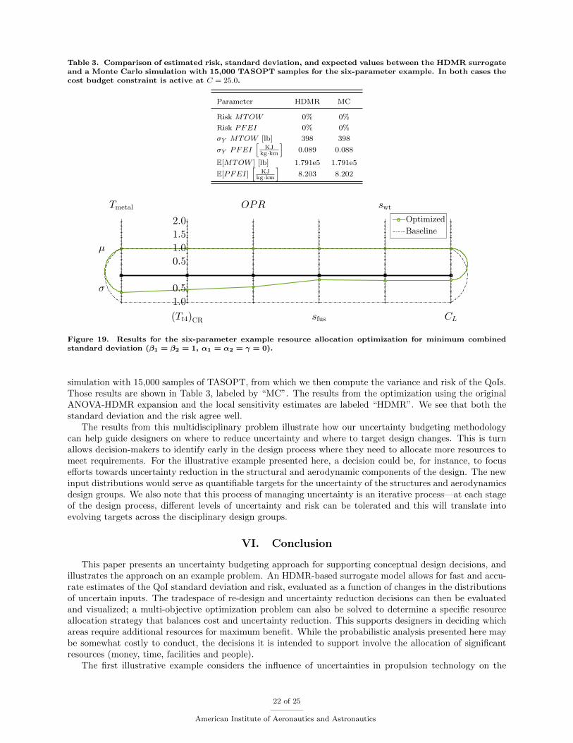
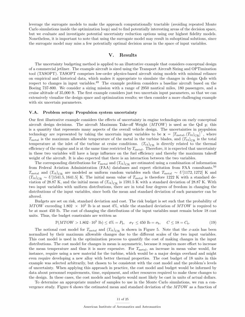
Table 3. Comparison of estimated risk, standard deviation, and expected values between the HDMR surrogateand a Monte Carlo simulation with 15,000 TASOPT samples for the six-parameter example. In both cases thecost budget constraint is active at C = 25.0.

Parameter HDMR MC

Risk MTOW 0% 0%

Risk PFEI 0% 0%

σY MTOW [lb] 398 398

σY PFEI[

KJkg·km

]0.089 0.088

E[MTOW ] [lb] 1.791e5 1.791e5

E[PFEI][

KJkg·km

]8.203 8.202

Tmetal

(Tt4)CR

OPR

sfus

swt

CL

µ

σ

0.5

1.0

1.5

2.0

0.5

1.0

Optimized

Baseline

Figure 19. Results for the six-parameter example resource allocation optimization for minimum combinedstandard deviation (β1 = β2 = 1, α1 = α2 = γ = 0).

simulation with 15,000 samples of TASOPT, from which we then compute the variance and risk of the QoIs.Those results are shown in Table 3, labeled by “MC”. The results from the optimization using the originalANOVA-HDMR expansion and the local sensitivity estimates are labeled “HDMR”. We see that both thestandard deviation and the risk agree well.

The results from this multidisciplinary problem illustrate how our uncertainty budgeting methodologycan help guide designers on where to reduce uncertainty and where to target design changes. This is turnallows decision-makers to identify early in the design process where they need to allocate more resources tomeet requirements. For the illustrative example presented here, a decision could be, for instance, to focusefforts towards uncertainty reduction in the structural and aerodynamic components of the design. The newinput distributions would serve as quantifiable targets for the uncertainty of the structures and aerodynamicsdesign groups. We also note that this process of managing uncertainty is an iterative process—at each stageof the design process, different levels of uncertainty and risk can be tolerated and this will translate intoevolving targets across the disciplinary design groups.

VI. Conclusion

This paper presents an uncertainty budgeting approach for supporting conceptual design decisions, andillustrates the approach on an example problem. An HDMR-based surrogate model allows for fast and accu-rate estimates of the QoI standard deviation and risk, evaluated as a function of changes in the distributionsof uncertain inputs. The tradespace of re-design and uncertainty reduction decisions can then be evaluatedand visualized; a multi-objective optimization problem can also be solved to determine a specific resourceallocation strategy that balances cost and uncertainty reduction. This supports designers in deciding whichareas require additional resources for maximum benefit. While the probabilistic analysis presented here maybe somewhat costly to conduct, the decisions it is intended to support involve the allocation of significantresources (money, time, facilities and people).

The first illustrative example considers the influence of uncertainties in propulsion technology on the

22 of 25


overall conceptual design of a commercial aircraft. The results highlight the kinds of useful conclusionsthat may be drawn from the analysis. In the case considered, the uncertainties in engine technology arerepresented by Tmetal—the maximum allowable temperature of the metal in the turbine—and (Tt4)CR—thetotal temperature at the inlet of the turbine. For the specific analysis case studied, (Tt4)CR has the largestinfluence on the uncertainty in the Maximum Take-off Weight (MTOW ) of the aircraft, while the interactionbetween Tmetal and (Tt4)CR is also responsible for a substantial part of the uncertainty in MTOW . Theresource allocation optimization leads to solutions for which the standard deviation of (Tt4)CR is reducedmore than the standard deviation of Tmetal, reflecting this higher sensitivity. A second example considersthe influence of system-wide uncertainties—in propulsion technology, material properties, and aerodynamicperformance parameters—on the overall conceptual aircraft design. The resource allocation optimizationshows that for the specific problem analyzed, the best strategy is to “spend” the uncertainty budget bytargeting a large uncertainty reduction in the material properties and the aerodynamic performance, andonly a small uncertainty reduction in the propulsion technology. This result would permit a design group toassign quantitative re-design targets to each disciplinary sub-group.

In both cases, the optimization yields strategies for which the changes in mean value are much smaller(relatively speaking) than the changes in input standard deviation. While the solutions found here reflectour particular problem set up and our chosen notional cost model, which places a large penalty on changesin the mean design point, this general result is consistent with many conceptual design problems where thecost of design changes are large. This paper aims not to recommend a specific aircraft design choice, butrather to provide a general methodology by which the designer can systematically explore these tradeoffsbetween design modifications and uncertainty reduction. We note that the bulk of multidisciplinary designoptimization methods focus on finding a single “optimal design”—even if uncertainty is included, the problemis still usually formulated as finding a single optimal design that minimizes some statistic of the QoI. However,the analysis enabled by our methodology suggests that focusing on uncertainty reduction rather than justdesign changes may be a more productive approach. A potential area of future work is to integrate theuncertainty budgeting methodology with a multi-level design formulation, such as ATC. This would enableconsideration of more complex systems, as well as greater insight into the role of cascading uncertaintiesbetween subsystem levels. Another area of future work is to develop more sophisticated budget models, suchas those that include correlation between cost and uncertainty budgets, and to use sensitivity results fromthe optimization solution to determine the relative gains of increasing or decreasing budget limits.

Acknowledgements

This work was supported in part by the NASA LEARN program through grant number NNX14AC73A,technical monitor Justin S. Gray, and by the United States Department of Energy Applied MathematicsProgram, Awards DE-FG02-08ER2585 and DE-SC0009297, program manager Steven Lee, as part of theDiaMonD Multifaceted Mathematics Integrated Capability Center.

References

1Haldar, A. and Mahadevan, S., Probability, Reliability and Statistical Methods in Engineering Design, John Wiley &Sons, Inc., New York, NY, 2000.

2Roy, C. J. and Oberkampf, W. L., “A Comprehensive Framework for Verification, Validation, and Uncertainty Quantifi-cation in Scientific Computing,” Computer Methods in Applied Mechanics and Engineering, Vol. 200, 2011, pp. 2131–2144.

3Mavris, D. N., Bandte, O., and DeLaurentis, D. A., “Robust Design Simulation: A Probabilistic Approach to Multidis-ciplinary Design,” Journal of Aircraft , Vol. 36, No. 1, 1999, pp. 298–307.

4Smith, R., Uncertainty Quantification: Theory, Implementation, and Applications, SIAM, Philadelphia, 2014.5Oberkampf, W. L., DeLand, S. M., Rutherford, B. M., Diegert, K. V., and Alvin, K. F., “Error and Uncertainty in

Modeling and Simulation,” Reliability Engineering and System Safety, Vol. 75, 2002, pp. 333–357.6Ang, A. H.-S. and Tang, W. H., Probability Concepts in Engineering: Emphasis on Applications to Civil and Environ-

mental Engineering, John Wiley & Sons, Inc., Hoboken, NJ, 2nd ed., 2007.7Kennedy, M. C. and O’Hagan, A., “Bayesian Calibration of Computer Models,” Journal of the Royal Statistical Society,

Series B , Vol. 63, No. 3, 2001, pp. 425–464.8Cacuci, D., Ionescu-Bujor, M., and Navon, I., Sensitivity And Uncertainty Analysis: Applications to Large-Scale Systems

(Volume II), Chapman & Hall, 2005.9Helton, J. C., Johnson, J. D., Sallaberry, C. J., and Storlie, C. B., “Survey of Sampling-Based Methods for Uncertainty

and Sensitivity Analysis,” Reliability Engineering and System Safety, Vol. 91, 2006, pp. 1175–1209.

23 of 25


10Aughenbaugh, J. M. and Paredis, C. J., “The Value of Using Imprecise Probabilities in Engineering Design,” Journal ofMechanical Design, Vol. 128, No. 4, 2006, pp. 969–979.

11Venter, G., Haftka, R. T., and Starnes, J. H., “Construction of Response Surface Approximations for Design Optimiza-tion,” AIAA Journal , Vol. 36, No. 12, 1998, pp. 2242–2249.

12Eldred, M. S., Giunta, A. A., and Collis, S. S., “Second-Order Corrections for Surrogate-Based Optimization with ModelHierarchies,” 10th AIAA/ISSMO Multidisciplinary Analysis and Optimization Conference, AIAA Paper 2004-4457 , Albany,NY, 2004.

13Simpson, T. W., Peplinski, J. D., Koch, P. N., and Allen, J. K., “Metamodels for Computer-Based Engineering Design:Survey and Recommendations,” Engineering with Computers, Vol. 17, No. 2, 2001, pp. 129–150.

14Alexandrov, N. M., Lewis, R. M., Gumbert, C. R., Green, L. L., and Newman, P. A., “Approximation and ModelManagement in Aerodynamic Optimization with Variable-Fidelity Models,” Journal of Aircraft , Vol. 38, No. 6, 2001, pp. 1093–1101.

15Queipo, N. V., Haftka, R. T., Shyy, W., Goel, T., Vaidyanathan, R., and Tucker, P. K., “Surrogate-based Analysis andOptimization,” Progress in Aerospace Sciences, Vol. 41, No. 1, 2005, pp. 1–28.

16Lee, S. H. and Chen, W., “A Comparative Study of Uncertainty Propagation Methods for Black-box-type Problems,”Structural and Multidisciplinary Optimization, Vol. 37, No. 3, 2009, pp. 239–253.

17Saltelli, A., Chan, K., and Scott, E. M., Sensitivity Analysis, John Wiley & Sons, Inc., New York, NY, 2000.18Homma, T. and Saltelli, A., “Importance Measures in Global Sensitivity Analysis of Nonlinear Models,” Reliability

Engineering & System Safety, Vol. 52, No. 1, 1996, pp. 1–17.19Sobol’, I. M., “Sensitivity Estimates for Nonlinear Mathematical Models,” Mathematical Modeling and Computational

Experiment , Vol. 1, No. 4, 1993, pp. 407–414.20Sobol’, I. M., “Theorems and Examples on High Dimensional Model Representation,” Reliability Engineering & System

Safety, Vol. 79, No. 2, 2003, pp. 187–193.21Chan, K., Saltelli, A., and Tarantola, S., “Sensitivity Analysis of Model Output: Variance-Based Methods Make the

Difference,” Proceedings of the 1997 Winter Simulation Conference, 1997.22Saltelli, A. and Bolado, R., “An Alternative Way to Compute Fourier Amplitude Sensitivity Test (FAST),” Computational

Statistics and Data Analysis, Vol. 26, 1998, pp. 445–460.23Liu, H., Chen, W., and Sudjianto, A., “Relative Entropy Based Method for Probabilistic Sensitivity Analysis in Engi-

neering Design,” Journal of Mechanical Design, Vol. 128, No. 2, 2006, pp. 326–336.24Knoll, F. and Vogel, T., Design for Robustness, IABSE (International Association for Bridge and Structural Engineering),

Zurich, Switzerland, 2009.25Taguchi, G., The System of Experimental Design: Engineering Methods to Optimize Quality and Minimize Costs (2

vols.), UNIPUB/Kraus International Publications and American Supplier Institute, White Plains, NY and Dearborn, MI, 1987.26Phadke, M. S., Quality Engineering Using Robust Design, Prentice Hall, Englewood Cliffs, NJ, 1989.27Chen, W., Allen, J. K., Tsui, K.-L., and Mistree, F., “Procedure for Robust Design: Minimizing Variations caused by

Noise Factors and Control Factors,” Journal of Mechanical Design, Vol. 118, No. 4, 1996, pp. 478–485.28Du, X., Sudjianto, A., and Chen, W., “An integrated framework for optimization under uncertainty using inverse reliability

strategy,” Journal of Mechanical Design, Vol. 126, No. 4, 2004, pp. 562–570.29Kim, H. M., Michelena, N. F., Papalambros, P. Y., and Jiang, T., “Target Cascading in Optimal System Design,” Journal

of Mechanical Design, Vol. 125, No. 3, 2003, pp. 474–480.30Kokkolaras, M., Mourelatos, Z. P., and Papalambros, P. Y., “Design optimization of hierarchically decomposed multilevel

systems under uncertainty,” Journal of mechanical design, Vol. 128, No. 2, 2006, pp. 503–508.31Kokkolaras, M., “Reliability Allocation in Probabilistic Design Optimization of Decomposed Systems using Analytical

Target Cascading,” 12th AIAA/ISSMO Multidisciplinary Analysis and Optimization Conference, Victoria, British Columbia,Canada, Paper No. AIAA-2008-6040 , September 10–12 2008.

32Chen, X., Molina-Cristobal, A., Guenov, M., Datta, V. C., and Riaz, A., “A Novel Method for Inverse UncertaintyPropagation,” EUROGEN 2015 , Glasgow, UK, September 14–16 2015.

33Padulo, M., Campobasso, M. S., and Guenov, M. D., “Novel uncertainty propagation method for robust aerodynamicdesign,” AIAA journal , Vol. 49, No. 3, 2011, pp. 530–543.

34Curran, C. and Willcox, K., “Sensitivity Analysis Methods for Mitigating Uncertainty in Engineering System Design,”56th AIAA/ASCE/AHS/ASC Structures, Structural Dynamics, and Materials Conference, Kissimee, FL, Paper No. AIAA-2015-0899 , January 5–9 2015.

35He, Q., Uncertainty and Sensitivity Analysis Methods for Improving Design Robustness and Reliability, Ph.D. thesis,Massachusetts Institute of Technology, June 2014.

36Torenbeek, E., Synthesis of subsonic airplane design : an introduction to the preliminary design, of subsonic generalaviation and transport aircraft, with emphasis on layout, aerodynamic design, propulsion, and performance, Delft UniversityPress Nijhoff Sold and distributed in the U.S. and Canada by Kluwer Boston, Delft The Hague Hingham, MA, 1982.

37Rabitz, H., Alis, O. F., Shorter, J., and Shim, K., “Efficient input-output model representations,” Computer PhysicsCommunications, Vol. 117, No. 1, 1999, pp. 11–20.

38Rabitz, H. and Alis, O. F., “General foundations of high-dimensional model representations,” Journal of MathematicalChemistry, Vol. 25, No. 2-3, 1999, pp. 197–233.

39Alıs, O. F. and Rabitz, H., “Efficient implementation of high dimensional model representations,” Journal of MathematicalChemistry, Vol. 29, No. 2, 2001, pp. 127–142.

40Wang, S.-W., Georgopoulos, P. G., Li, G., and Rabitz, H., “Random sampling-high dimensional model representation(RS-HDMR) with nonuniformly distributed variables: application to an integrated multimedia/multipathway exposure anddose model for trichloroethylene,” The Journal of Physical Chemistry A, Vol. 107, No. 23, 2003, pp. 4707–4716.

24 of 25


41Li, G. and Rabitz, H., “General formulation of HDMR component functions with independent and correlated variables,”Journal of Mathematical Chemistry, Vol. 50, No. 1, 2012, pp. 99–130.

42Sobol, I. M., “Theorems and examples on high dimensional model representation,” Reliability Engineering & SystemSafety, Vol. 79, No. 2, 2003, pp. 187–193.

43Li, G., Wang, S.-W., and Rabitz, H., “Practical approaches to construct RS-HDMR component functions,” The Journalof Physical Chemistry A, Vol. 106, No. 37, 2002, pp. 8721–8733.

44Saltelli, A., Global sensitivity analysis : the primer , John Wiley, Chichester, England Hoboken, NJ, 2008.45Sobol, I. M., “Global sensitivity indices for nonlinear mathematical models and their Monte Carlo estimates,” Mathematics

and computers in simulation, Vol. 55, No. 1-3, 2001, pp. 271–280.46Shapiro, A., Dentcheva, D., and Ruszczynski, A., Lectures on stochastic programming. Modeling and theory, Vol. 9 of

MPS/SIAM Series on Optimization, Society for Industrial and Applied Mathematics (SIAM), Philadelphia, PA; MathematicalProgramming Society (MPS), Philadelphia, PA, 2nd ed., 2014.

47Opgenoord, M. M. J., Uncertainty Budgeting Methods for Conceptual Aircraft Design, SM thesis, Massachusetts Instituteof Technology, Cambridge, MA, February 2016.

48Li, G., Hu, J., Wang, S.-W., Georgopoulos, P. G., Schoendorf, J., and Rabitz, H., “Random sampling-high dimensionalmodel representation (RS-HDMR) and orthogonality of its different order component functions,” The Journal of PhysicalChemistry A, Vol. 110, No. 7, 2006, pp. 2474–2485.

49Drela, M., “N3 Aircraft Concept Designs and Trade Studies – Appendix,” Tech. Rep. NASA CR-2010-216794/VOL2,2010.

50Amaral, S., A Decomposition-Based approach to Uncertainty Quantification of Multicomponent Systems, Ph.D. thesis,Massachusetts Institute of Technology, June 2015.

51Kanukolanu, D., Lewis, K., and Winer, E., “A multidimensional visualization interface to aid in trade-off decisions duringthe solution of coupled subsystems under uncertainty,” Journal of Computing and Information Science in Engineering, Vol. 6,No. 3, 2006, pp. 288–299.

52Svanberg, K., “A class of globally convergent optimization methods based on conservative convex separable approxima-tions,” SIAM journal on optimization, Vol. 12, No. 2, 2002, pp. 555–573.

53Johnson, S. G., “The NLopt nonlinear-optimization package,” http://ab-initio.mit.edu/nlopt.

25 of 25


uncertainty budgeting in system design...y standard deviation of qoi y;b budget on the standard...

Documents