1 News about the future and �uctuations

� old idea: expectations drive business cycle

� uncertainty about the economy�s fundamentals, which will determine thelong run equilibrium

� partial equilibrium ideas:

� consumption: permanent income hypothesis future income expecta-tions matter for consumption decisions

� investment: high expected returns

� problem: how to �t these ideas in general equilibrium setup

1.1 Evidence

� basic fundamental for long-run growth: TFP

� can expectations about long-run TFP drive cycle?

� how to measure expectations?

� Beaudry and Portier (2006): use the stock-market

"�TFPt�St

#=

"a11 (L) a12 (L)a21 (L) a22 (L)

# ""1t"2t

#

Two identi�cation approaches:

1. Short run:

a12;0 = 0:

2. Long run:

a12 (1) = 0:

0

5 10 15 200-0.1

0.1

0.2

0.3

0.4

0.5

0.6

0.7

0.8 11

10

9

8

7

6

50 5 10 15 20

quarters quarters

% d

evia

tion

% d

evia

tion

Impulse responses to shocks ε2 and ε1 in the (TFP, SP) VAR

TFP Stock prices

~

Image by MIT OpenCourseWare. Adapted from Figure 2 in Beaudry, Paul, and Franck Portier. “Stock Prices, News, and Economic Fluctuations.’’ NationalBureau of Economic Research Working Paper No. 10548, June 2004.

0 2 4 6 8 10 12 00

2 4 6 8 10 12

0 2 4 6 8 10 12 0 2 4 6 8 10 12

0.5

0.45

0.4

0.35

0.3

0.25

0.2

0.15

0.1

1.4

1.2

1

0.8

0.6

0.4

0.2

0

1.4

1.2

1

0.8

0.6

0.4

0.2

0

3

2.5

2

1.5

1

0.5

Consumption (a)

quartersquarters

quarters quarters

% d

evia

tion

% d

evia

tion

% deviation

% deviation

The figure displays the response of consumption, investment, output (measured as C + I) and hoursto a unit ε2 shock (the shock that does not have instantaneous impact on TFP in the short run identification). The unit of the vertical axis is percentage deviation from the situation without shock. (See the main text for more details)

Impulse responses to ε2 in the baseline (TFP, SP) VAR

Hoursoutput (C+I)

Image by MIT OpenCourseWare. Adapted from Figure 8 in Beaudry, Paul, and Franck Portier. “Stock Prices, News, and Economic Fluctuations.’’National Bureau of Economic Research Working Paper No. 10548, June 2004.

0.70.60.50.40.30.20.1

0

5 10 15 20 25 30 35 400

-0.1-0.2

5 10 15 20 25 30 35 400

10

8

6

4

2

0

-2

-15 10 15 20 25 30 35 400

1.4

1.2

1

0.8

0.6

0.4

0.2

0

5 10 15 20 25 30 35 400

12

10

8

6

4

2

0

-25 10 15 20 25 30 35 400

1

0.8

0.6

0.40.2

0

-0.2

-0.4

5 10 15 20 25 30 35 400

1.41.2

10.80.60.40.2

0-0.2

5 10 15 20 25 30 35 400

1.81.61.41.2

10.80.60.40.2

5 10 15 20 25 30 35 400

1.4

1.2

1

0.8

0.6

0.4

0.2

0

% D

evia

tion

% D

evia

tion

% D

evia

tion

% D

evia

tion

% D

evia

tion

% D

evia

tion

% D

evia

tion

% D

evia

tion

quarters quarters quarters quarters

quarters quarters quarters quarters

TFP Stock prices Consumption Hours

TFP Stock prices Consumption Hours

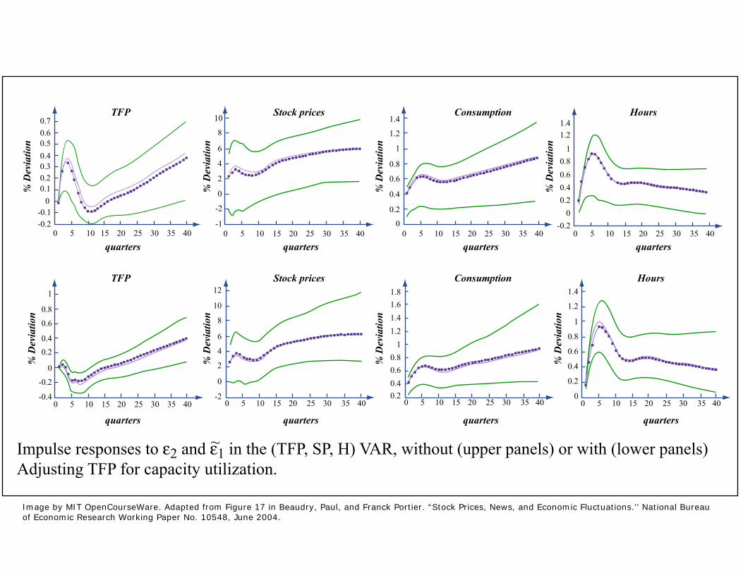
Impulse responses to ε2 and ε1 in the (TFP, SP, H) VAR, without (upper panels) or with (lower panels) Adjusting TFP for capacity utilization.

~

Image by MIT OpenCourseWare. Adapted from Figure 17 in Beaudry, Paul, and Franck Portier. “Stock Prices, News, and Economic Fluctuations.’’ National Bureauof Economic Research Working Paper No. 10548, June 2004.

1

0.8

0.6

0.4

0.2

00 5 10 15 20 25 30

0

0.1

0.2

0.3

0.4

0.5

0.6

0.7

0.8

0.9

0 5 10 15 20 25 30

Shar

e of

F.E

.V.

Shar

e of

F.E

.V.

0.1

1

0.9

0.8

0.7

0.6

0.5

0.4

0.3

0.2

0 5 10 15 20 25 30

Shar

e of

F.E

.V.

quarters

0.1

1

0.9

0.8

0.7

0.6

0.5

0.4

0.3

0.2

0 5 10 15 20 25 30

Shar

e of

F.E

.V.

quarters

quarters quarters

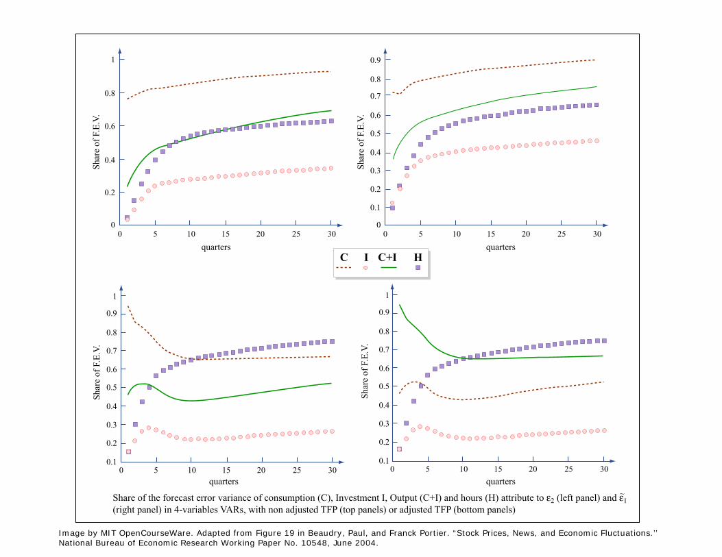
Share of the forecast error variance of consumption (C), Investment I, Output (C+I) and hours (H) attribute to ε2 (left panel) and ε1 (right panel) in 4-variables VARs, with non adjusted TFP (top panels) or adjusted TFP (bottom panels)

C I HC+I

~

Image by MIT OpenCourseWare. Adapted from Figure 19 in Beaudry, Paul, and Franck Portier. “Stock Prices, News, and Economic Fluctuations.’’National Bureau of Economic Research Working Paper No. 10548, June 2004.

Main conclusions:

� both identi�cations give similar shocks

� response of C and Y builds up, then permanent

� response of H has hump then dies out slowly

1.2 Neoclassical growth model

Preferences

E1Xt=0

�tU (Ct; Nt)

Technology

Ct +Kt � (1� �)Kt�1 � AtF (Kt�1; Nt)

� what happens when agents receive news about future At+s?

� what type of cycles does this generate?

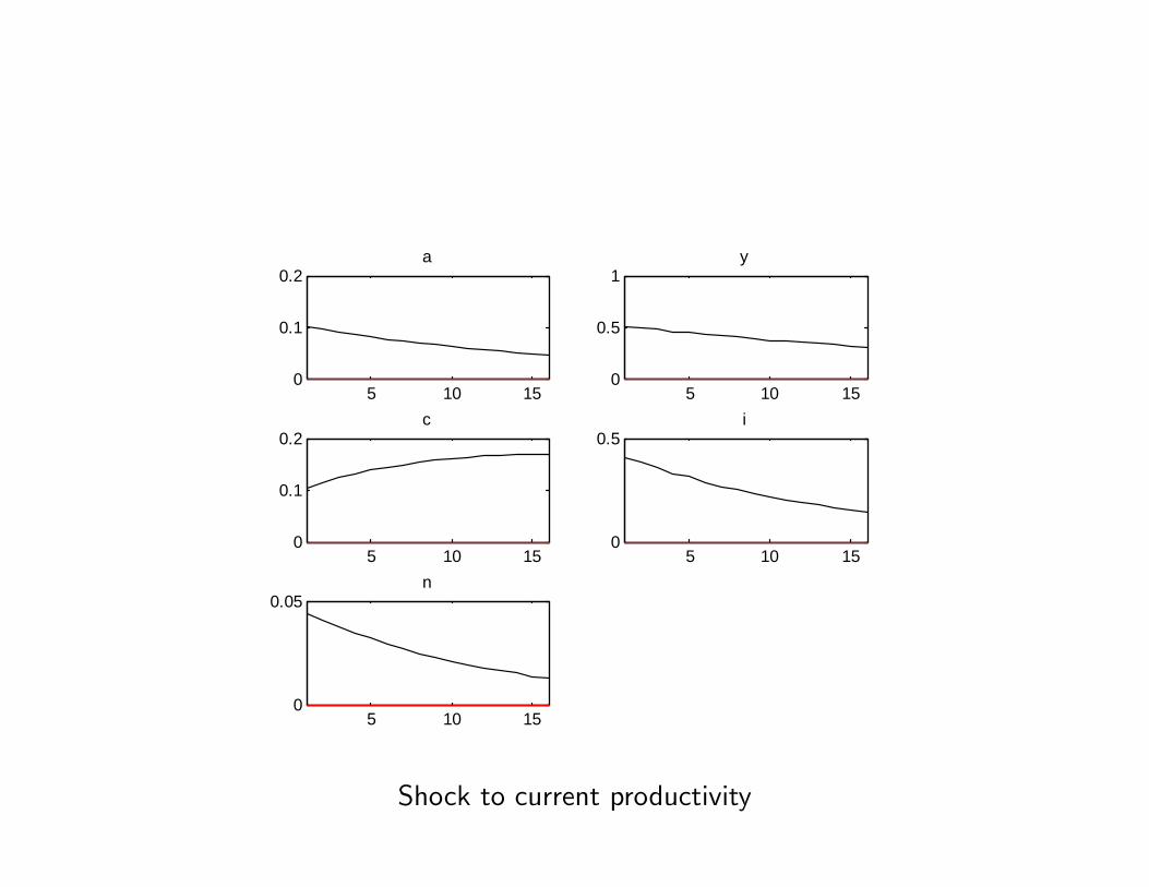
Basic parametrization

U (Ct; Nt) = logCt �1

1 + �N1+�t

AtF (Kt�1; Nt) = AtK�t�1N

1��t

At = eat

at = �at�1 + �t

� = 0:99

� = 1

� = 0:36

� = 0:95

� = 0:025

5 10 150

0.1

0.2a

5 10 150

0.5

1y

5 10 150

0.1

0.2c

5 10 150

0.5i

5 10 150

0.05n

Shock to current productivity

� Now introduce news about the future

� Simplest way: agents observe shock realization T periods in advance

at = �at�1 + �t�T

� What happens at the time of the announcement?

� Consumption increases, investment and hours fall!

� Danthine, Donaldson and Johnsen (1997), Beaudry and Portier (2005):nothing that looks like business cycles.

2 4 6 8 10­0.2

0

0.2a

2 4 6 8 10­1

0

1y

2 4 6 8 100

0.1

0.2c

2 4 6 8 10­1

0

1i

2 4 6 8 10­0.2

0

0.2n

1.2.1 Mechanism

Basic mechanism driven by intra-temporal optimality condition

(1� �) 1CtAtK

�t�1N

��t = N

�t

or (in terms of real wages)

1

CtWt = N

�t

together with the resource constraint

It + Ct = AtK��1t�1 N

1��t

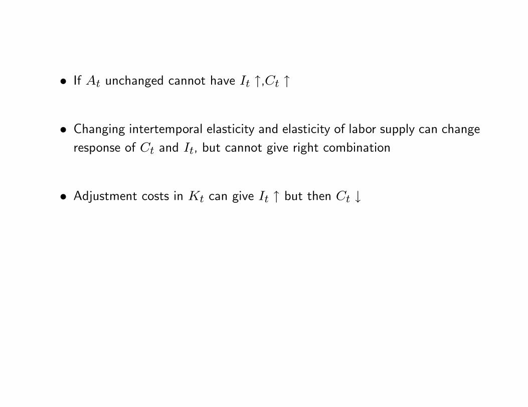
� If At unchanged cannot have It ",Ct "

� Changing intertemporal elasticity and elasticity of labor supply can changeresponse of Ct and It, but cannot give right combination

� Adjustment costs in Kt can give It " but then Ct #

� No hope for neoclassical model with news about the future?

� Several attempts

� Jaimovich and Rebelo (2006): three ingredients

� adjustment costs in investment

� variable capacity utilization

� preferences with �weak wealth e¤ects on labor supply�

3

2.5

2

1.5

1

0.5

00 2 4 6 8 10

Consumption

3

Hours

OutputInvestment

2.5

2

1.5

1

0.5

00 2 4 6 8 10

00 2

2

4

4

6

6

8

8

10

10

00.5

0 2

1

4

21.5

6

32.5

8

3.5

10

4

Response to TFP News Shock, Our Model

Percentage deviations from steady state

Image by MIT OpenCourseWare. Adapted from Figure 2 in Jaimovich, Nir, and Sergio Rebelo. "Can News about the Future Drive the Business Cycle?"National Bureau of Economic Research Working Paper No. 12537, September 2006.

Preferences

X�t

�Ct �N�tXt

�1�� � 11� �

� Xt is a geometric discounted average of past consumption levels

Xt = C t X

1� t�1 :

� The parameter 2 [0; 1]: speed at which the wealth e¤ect kicks in

� Suppose Xt � 1 then quasi-linear (GHH)

Wt = �N��1t

no income e¤ect here. Inconsistent with LR growth

� Here income e¤ect that phases in slowly

� In the long run

Wt = �N��1t Ct

Simplistic interpretation:

1. quasi-linear in short run: no income e¤ect

2. log in the long run: income and substitution cancel

but 1 is wrong!

Decomposition: income e¤ect

X�t

�Ct �N�tXt

�1�� � 11� �

XR�t (Ct �WNt) = B0

� Suppose real wage constant at W , interest rate constant at R = 1=�

� e¤ects of an increase in B0

1

0.8

0.6

0.4

0.2

0

-0.2

-0.4

-0.6

2 4 6 8 10 12 14 16 18 20 22 24Periods

% D

evia

tions

from

Ste

ady

Stat

e

Response of Hours - Income Effect

GHHgamma = 0.01 gamma = 0.5

gamma = 0.6

gamma = 0.7

gamma = 0.8

gamma = 0.9

gamma = KPR

gamma = 0.05

gamma = 0.1

gamma = 0.2

gamma = 0.3

gamma = 0.4

Image by MIT OpenCourseWare.

Mechanism

�rst order condition for labor supply in the following form

�tWt = �XtN��1t ;

and

�t =

�Ct �N�tXt

��� � �t C �1t X1� t�

Ct �N�tXt��� ;

where �t is a complicated forward looking object.

Agents forecast that work will be painful in the future, so they work more today

1.2.2 Habits and labor supply

Christiano, Ilut, Motto and Rostagno

E1Xt=0

�t log (Ct � bCt�1)�

1

1 + �N1+�t

!(habit)

Kt = (1� �)Kt�1 +

0@1� a2

It

It�1

!21A It (CEE Adj. Costs)Yt = AtK

�t N

1��t = It + Ct

At = eat

at = �at�1 + �t�T

0.7 0.9

0.8

0.7

0.6

0.5

0.4

0.3

0.2

0.6

0.5

0.4

0.3

0.2

0.1

2 24 46 68 8

Output Investment Consumption

Pk

Perc

ent

Perc

ent

Perc

ent

Perc

ent

0.4

0.2

0

-0.2

-0.4

-0.62 4 6 8

Perc

ent

2 4 6 8

0.6

0.5

0.4

0.3

0.2

0.1

0

2 4 6 8

1000

800

600

400

200

0

-200

2 4 6 8

1.5

1

0.5

0

-0.5

Hours workedRiskfree rate with payoff in

t+1 (annual)B

ass p

oint

s

t t t

ttt

Perturbed RBC ModelBaseline RBC Model

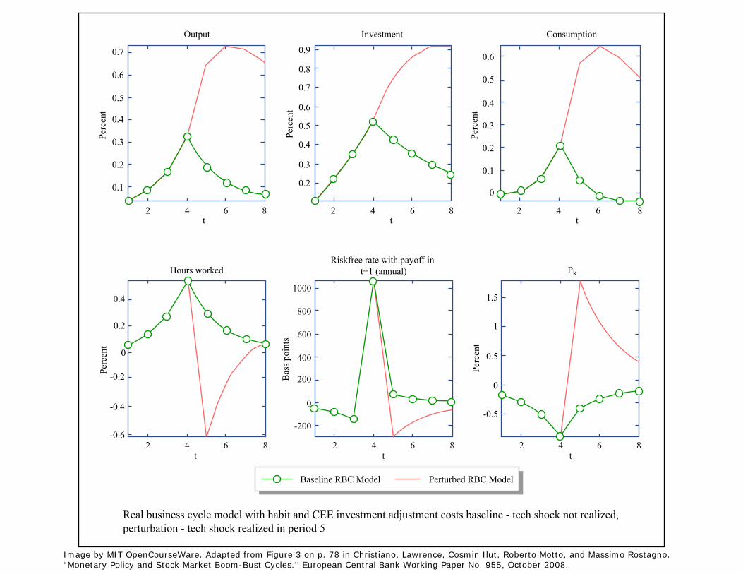
Real business cycle model with habit and CEE investment adjustment costs baseline - tech shock not realized, perturbation - tech shock realized in period 5

Image by MIT OpenCourseWare. Adapted from Figure 3 on p. 78 in Christiano, Lawrence, Cosmin Ilut, Roberto Motto, and Massimo Rostagno.“Monetary Policy and Stock Market Boom-Bust Cycles.’’ European Central Bank Working Paper No. 955, October 2008.

Perc

ent

0.05

0.1

0.15

0.2

0.25

0.3

Output

t2 4 6 8

Perturbed RBC Model Baseline RBC Model

2

Perc

ent

0.10.05

0.150.2

0.250.3

0.350.4

0.450.5

4

Hours worked

t6 8

Bas

is p

oint

s

0

200

400

600

800

1000

Riskfree rate with payoffin t+1 (annual)

t2 4 6 8

Perc

ent

-0.8

-0.7

-0.5-0.6

-0.2

-0.3

-0.4

Pk

t2 4 6 8

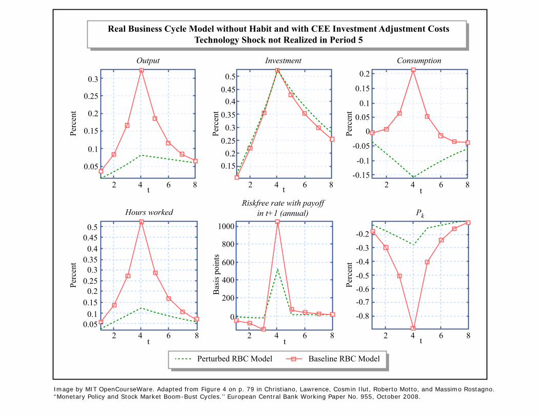
Real Business Cycle Model without Habit and with CEE Investment Adjustment CostsTechnology Shock not Realized in Period 5

Perc

ent

0.150.2

0.25

0.350.3

0.40.45

0.5

Investment

t2 4 6 8 2

Perc

ent

-0.15

-0.1

0

0.1

0.05

-0.05

0.15

0.2

4

Consumption

t6 8

Image by MIT OpenCourseWare. Adapted from Figure 4 on p. 79 in Christiano, Lawrence, Cosmin Ilut, Roberto Motto, and Massimo Rostagno.“Monetary Policy and Stock Market Boom-Bust Cycles.’’ European Central Bank Working Paper No. 955, October 2008.

Perc

ent

-0.1-0.05

00.050.1

0.150.2

0.250.3

Output

t2 4 6 8

2

Perc

ent

-0.1

0

0.1

0.2

0.3

0.4

0.5

4

Hours worked

t6 8

Perc

ent

-0.4-0.3-0.2-0.1

00.10.20.30.40.5

Investment

t2 4 6 8 2

Perc

ent

-0.05

0

0.05

0.1

0.15

0.2

4

Consumption

t6 8

Bas

is p

oint

s

0

200

400

600

800

1000

Riskfree rate with payoffin t+1 (annual)

t2 4 6 8

Perc

ent

-0.8

-0.6

-0.4

-0.2

0

0.2Pk

t2 4 6 8

Perturbed RBC Model Baseline RBC Model

Real Business Cycle Model with Habit and Without Investment Adjustment Costs TechnologyShock not Realized in Period 5

Image by MIT OpenCourseWare.Adapted from Figure 5 on p. 80 in Christiano, Lawrence, Cosmin Ilut, Roberto Motto, and Massimo Rostagno.“Monetary Policy and Stock Market Boom-Bust Cycles.’’ European Central Bank Working Paper No. 955, October 2008.

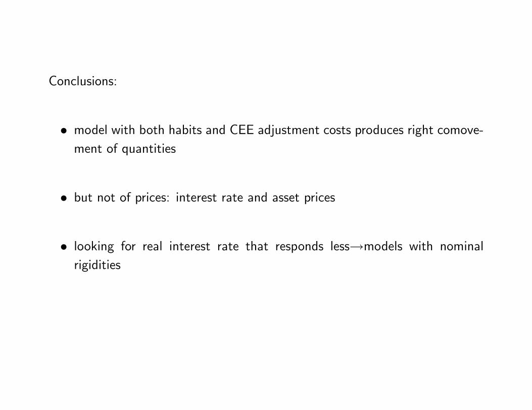
Conclusions:

� model with both habits and CEE adjustment costs produces right comove-ment of quantities

� but not of prices: interest rate and asset prices

� looking for real interest rate that responds less!models with nominalrigidities

Importance of habit formation

�tWt = N�t

�t =1

Ct � bCt�1� �bEt

"1

Ct+1 � bCt

#

� high consumption in the future increases incentive to work today.

� wealth e¤ects here? See problem set

1.3 Nominal rigidities

� two period economy

� households of consumers-producers

� monopolistic competition, price-setting

� uncertainty about productivity

� preferences2Xt=1

�t logCit �

�

1 + �N1+�it

!;

Cit is the CES aggregate

Cit =

Z 10C��1�ijt di

! ���1

;

with � > 1

� Technology

Yit = AtNit:

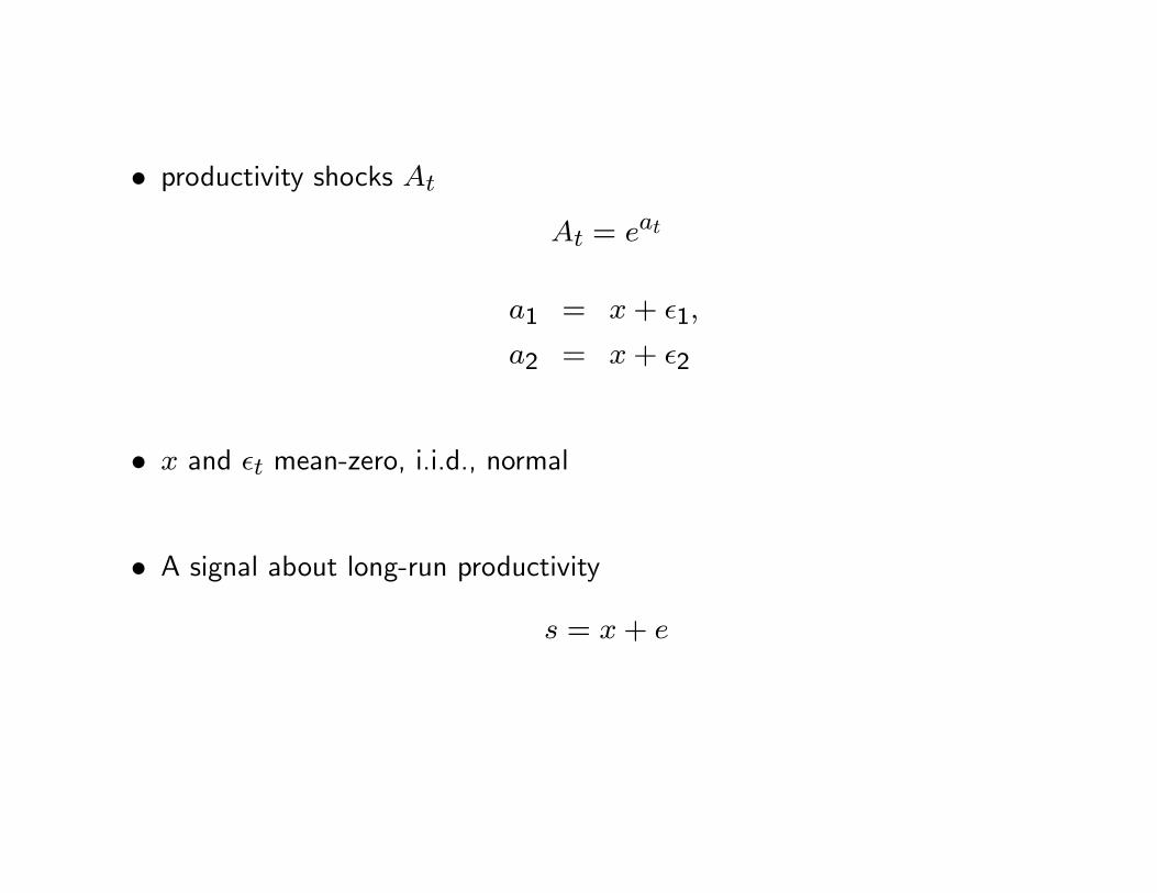
� productivity shocks AtAt = e

at

a1 = x+ �1;

a2 = x+ �2

� x and �t mean-zero, i.i.d., normal

� A signal about long-run productivity

s = x+ e

� nominal balances with central bank at nominal rate R

� household set Pit then consumers buy

� intertemporal BC

(P2Ci2 � Pi2Yi2) +R � (P1Ci1 � Pi1Yi1) � 0;

� Pt is the price index

Pt =�Z

P 1��it di

� 11��

:

Flexible price equilibrium

� optimality for price-setting

(1� �) 1

PtCit

PitYitPit

+ ��1

At

YitPitN�it = 0:

� symmetric equilibrium, Yt = AtNt, this condition gives

Nt =�� � 1��

� 11+�

= 1

(choosing � = (� � 1) =�).

� quantitiesCt = Yt = At:

� what about consumers�decisions?

� consumer Euler equation

1

C1= RE

"P1P2

1

C2ja1; s

#

� Ct = At log-normal

r + p1 � E [p2ja1; s] = E [a2ja1; s]� a1 �1

2V ar [a2ja1; s] :

� all changes in E [y2] go to the real interest rate

� notice role of p1: neutralizes r

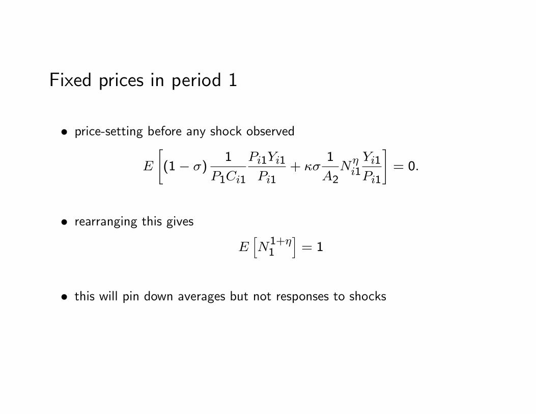
Fixed prices in period 1

� price-setting before any shock observed

E

"(1� �) 1

P1Ci1

Pi1Yi1Pi1

+ ��1

A2N�i1Yi1Pi1

#= 0:

� rearranging this gives

EhN1+�1

i= 1

� this will pin down averages but not responses to shocks

� quantities: equilibrium in period 2 identical

� in period 1 now Euler equation (set p2 = 0)

c1 = E [a2ja1; s]�1

2V ar [a2ja1; s]� r � p1:

� suppose r �xed, p1 �xed by assumption

� now �sentiment shocks�a¤ect consumption

0

0.2

0.4

0.60.8

1

5 10 15 20

Perc

ent

0.5

1

1.5

5 10 15 20

Perc

ent

Output

0

0.5

1

5 10 15 20

Perc

ent

Hours worked

Investment

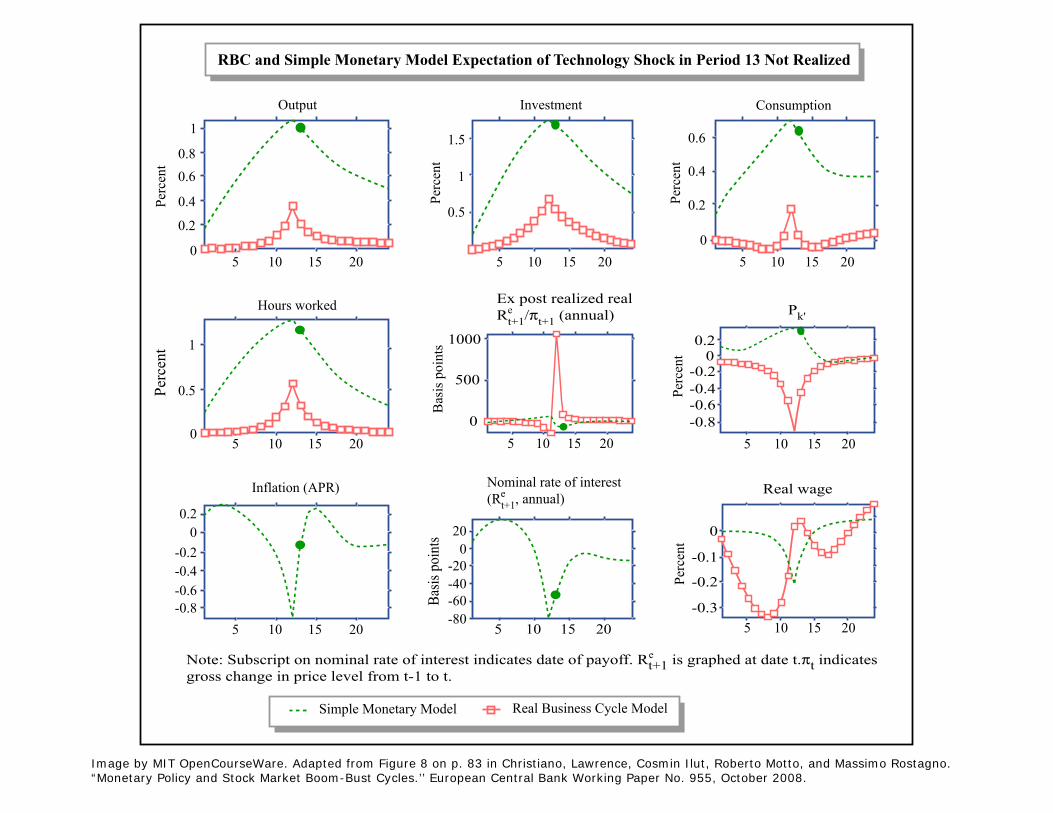
RBC and Simple Monetary Model Expectation of Technology Shock in Period 13 Not Realized

0

500

1000

5 10 15 20B

asis

poi

nts

Pk'

0.2

0

0.4

0.6

5 10 15 20

Perc

ent

Consumption

Simple Monetary Model Real Business Cycle Model

-0.6-0.8

-0.4-0.2

00.2

5 10 15 20

Inflation (APR)

-80-60-40-20

020

5 10 15 20

Basis

poi

nts

-0.8-0.6-0.4-0.2

00.2

5 10 15 20

Perc

ent

Real wage

-0.3

-0.2

-0.1

0

5 10 15 20

Perc

ent

Nominal rate of interest(Rt+1, annual)e

Ex post realized realRt+1/πt+1 (annual)e

eNote: Subscript on nominal rate of interest indicates date of payoff. Rt+1 is graphed at date t.πt indicatesgross change in price level from t-1 to t.

Image by MIT OpenCourseWare. Adapted from Figure 8 on p. 83 in Christiano, Lawrence, Cosmin Ilut, Roberto Motto, and Massimo Rostagno.“Monetary Policy and Stock Market Boom-Bust Cycles.’’ European Central Bank Working Paper No. 955, October 2008.

� pin down p1EhN1+�1

i= E

he(1+�)(y1�a1)

i= 1;

� thanks to log-normality this equation can be solved explicitly and gives

�r � p1 �1

2V ar [a2ja1; s] +

1

2(1 + �) (� + � � 1)2 �2x +

+1

2(1 + �) (� � 1)2 �2� +

1

2(1 + �) �2�2e = 0

� where

E [a2ja1; s] = �a1 + �s

� simple implication anticipated changes in r are neutral

� if instead we follow rule, e.g.

r = �0 + �1y1

then economy response changes

� we�ll go back to monetary policy

MIT OpenCourseWarehttp://ocw.mit.edu

14.461 Advanced Macroeconomics IFall 2009

For information about citing these materials or our Terms of Use, visit: http://ocw.mit.edu/terms.