uncertainties of predictions from parton distribution

PHYSICAL REVIEW D, VOLUME 65, 014013

Uncertainties of predictions from parton distribution functions. II. The Hessian method

J. Pumplin, D. Stump, R. Brock, D. Casey, J. Huston, and J. KalkDepartment of Physics and Astronomy, Michigan State University, East Lansing, Michigan 48824

H. L. LaiDepartment of Physics and Astronomy, Michigan State University, East Lansing, Michigan 48824

and Ming-Hsin Institute of Technology, Hsin-Chu, Taiwan

W. K. TungDepartment of Physics and Astronomy, Michigan State University, East Lansing, Michigan 48824

and Theory Division, CERN, Geneva, Switzerland~Received 1 April 2001; published 12 December 2001!

We develop a general method to quantify the uncertainties of parton distribution functions and their physicalpredictions, with emphasis on incorporating all relevant experimental constraints. The method uses the Hessianformalism to study an effective chi-squared function that quantifies the fit between theory and experiment. Keyingredients are a recently developed iterative procedure to calculate the Hessian matrix in the difficult globalanalysis environment, and the use of parameters defined as components along appropriately normalized eigen-vectors. The result is a set of 2D eigenvector basis parton distributions~whered'16 is the number of partonparameters! from which the uncertainty on any physical quantity due to the uncertainty in parton distributionscan be calculated. We illustrate the method by applying it to calculate uncertainties of gluon and quarkdistribution functions,W boson rapidity distributions, and the correlation betweenW andZ production crosssections.

DOI: 10.1103/PhysRevD.65.014013 PACS number~s!: 12.38.2t

ntta

soon

dra

risean

ra

cesiv

cecsuich

sr-

ade

ofDg

ofteld’sndalri-bal

m,c-ri-

k-e

odmu-isby

eD

ofor

elynd

I. INTRODUCTION

The partonic structure of hadrons plays a fundamerole in elementary particle physics. Interpreting experimendata according to the standard model~SM!, precision mea-surement of SM parameters, and searches for signalphysics beyond the SM, all rely on the parton picturehadronic beam particles that follows from the factorizatitheorem of quantum chromodynamics~QCD!. The partondistribution functions ~PDF’s! are nonperturbative—anhence at present uncalculable—functions of momentum ftion x at a low-momentum transfer scaleQ0. They are deter-mined phenomenologically by a global analysis of expemental data from a wide range of hard-scattering procesusing perturbative QCD to calculate the hard scatteringto determine the dependence of the PDF’s onQ by therenormalization-group based evolution equations.

Considerable progress has been made in several paefforts to improve our knowledge of the PDF’s@1–3#, butmany problems remain open. In the conventional approaspecific PDF sets are constructed to represent the ‘‘bestmate’’ under various input assumptions, including selectvariations of some of the parameters@4–6#. From these re-sults, however, it is impossible to reliably assess the untainties of the PDF’s or, more importantly, of the physipredictions based on PDF’s. The need to quantify thosecertainties for precision SM studies and new physsearches in the next generation of collider experimentsstimulated much interest in developing new approachethis problem@7,8#. Several attempts to quantify the unce

0556-2821/2001/65~1!/014013~17!/$20.00 65 0140

all

off

c-

-s,d

llel

h,ti-

e

r-

n-sasto

tainties of PDF’s in a systematic manner have been mrecently@9–13#.

The task is difficult because of the diverse sourcesexperimental and theoretical uncertainty in the global QCanalysis. In principle, the natural framework for studyinuncertainties is that of the likelihood function@12,14,15#. Ifall experimental measurements were available in the formmutually compatible probability functions for candidatheory models, then the combined likelihood function wouprovide the probability distribution for the possible PDFthat enter the theory. From this, all physical predictions atheir uncertainties would follow. Unfortunately, such idelikelihood functions are rarely available from real expements. To begin with, most published data sets used in gloanalysis provide only effective errors in uncorrelated foralong with a single overall normalization uncertainty. Seondly, published errors for some well-established expements appear to fail standard statistical tests, e.g., thex2 perdegree of freedom, may deviate significantly from 1.0, maing the data set quite ‘‘improbable.’’ In addition, when thfew experiments that are individually amenable to likelihoanalysis are examined together, they appear to demandtually incompatible PDF parameters. A related problemthat the theoretical errors are surely highly correlated anddefinition poorly known. All these facts of life make thidealistic approach impractical for a real-world global QCanalysis.

The problems that arise in combining a large numberdiverse experimental and theoretical inputs with uncertaininconsistent errors are similar to the problems routinfaced in analyzing systematic errors within experiments, a

©2001 The American Physical Society13-1

afo

ab

en

udnsi

tin

ssos

he

th

im

e-thpi

d-

st

aer-hetoe

ar

mfiei-hontp

tethfonzeth

nethh

tothisCDies

aly-rent

-uts-andion

aryies

toos-

er-datathe

t toeseueour

edeO

s

ons

r

theof

J. PUMPLINet al. PHYSICAL REVIEW D 65 014013

in averaging data from measurements that are margincompatible@16#. Imperfections of data sets in the form ounknown systematic errors or unusual fluctuations—both—are a common occurrence. They need not necessdestroy the value of those data sets in a global analysis;we must adapt and expand the statistical tools we usanalyze the data, guided by reasonable physics judgeme

In this paper we develop a systematic procedure to stthe uncertainties of PDF’s and their physics predictiowhile incorporating all the experimental constraints usedthe previous CTEQ analysis@1#. An effective x2 function,called xglobal

2 , is used not only to extract the ‘‘best fit,’’ bualso to explore the neighborhood of the global minimumorder to quantify the uncertainties, as is done in the claerror matrix approach. Two key ingredients make this psible: ~i! a recently established iterative procedure@17# thatyields a reliable calculation of the Hessian matrix in tcomplex global analysis environment, and~ii ! the use of ap-propriately normalized eigenvectors to greatly improveaccuracy and utility of the analysis.

The Hessian approach is based on a quadratic approx

tion to xglobal2 in the neighborhood of the minimum that d

fines the best fit. It yields a set of PDF’s associated witheigenvectors of the Hessian, which characterize the PDFrameter space in the neighborhood of the global minimuma process-independentway. In a companion paper, referreto here as ‘‘the preceding paper’’@18#, we present a complementary process-dependent method that studiesxglobal

2 as afunction of whatever specific physical variable is of intereThat approach is based on the Lagrange multiplier~LM !method@17#, which does not require a quadratic approximtion to xglobal

2 , and hence is more robust; but, being focuson a single variable~or a few variables in a generalized fomulation! it does not provide complete information about tneighborhood of the minimum. We use the LM methodverify the reliability of the Hessian calculations, as discussin Sec. V. Further tests of the quadratic approximationdescribed in Appendix B.

The outline of the paper is as follows. In Sec. II we sumarize the global analysis that underlies the study, and dethe functionxglobal

2 that plays the leading role. In Sec. III wexplore the quality of fit in the neighborhood of the minmum. We derive the eigenvector basis sets, and showthey can be used to calculate the uncertainty on any quathat depends on the parton distributions. In Sec. IV we apthe formalism to derive uncertainties of the PDF parameand of the PDF’s themselves. In Sec. V we illustratemethod further by finding the uncertainties on predictionsthe rapidity distribution ofW production, and the correlatiobetweenW andZ production cross sections. We summariour results in Sec. VI. Two appendixes provide details onestimate of overall tolerance for the effectivexglobal

2 function,and on the validity of the quadratic approximation inherein the Hessian method. Two further appendixes supplyplicit tables of the coefficients that define the best fit andeigenvector basis sets. The mathematical methods usedhave been described in detail in@17#. Some preliminary re-sults have also appeared in@7,8#.

01401

lly

rrilyuttot.y,

n

ic-

e

a-

ea-n

.

-d

de

-ne

witylyrser

e

tx-eere

II. GLOBAL QCD ANALYSIS AND EFFECTIVE CHISQUARED

Global x2 analysis is a practical and effective waycombine a large number of experimental constraints. Insection, we describe the main features of the global Qanalysis, and explain how we quantify its uncertaintthrough the behavior ofxglobal

2 .

A. Experimental and theoretical inputs

We use the same experimental input as the CTEQ5 ansis @1#: 15 data sets on neutral-current and charged-curdeep inelastic scattering~DIS!, Drell-Yan lepton pair produc-tion, forward backward lepton asymmetry fromW produc-tion, and highpT inclusive jets, as listed in Table I of Appendix A. The total number of data points is 1295, after csuch asQ.2 GeV andW.4 GeV in DIS designed to reduce the influence of power-law suppressed correctionsother sources of theoretical error. The experimental precisand the information available on systematic errors vwidely among the experiments, which presents difficultfor the effort to quantify the uncertainties of the results.

The theory input is next-to-leading-order~NLO! perturba-tive QCD. The theory has systematic uncertainties dueuncalculated higher-order QCD corrections, including psible resummation effects near kinematic boundaries, powsuppressed corrections, and nuclear effects in neutrinoon heavy targets. These uncertainties—even more thanexperimental ones—are difficult to quantify.

The theory contains free parameters$ai%5$a1 , . . . ,ad%defined below that characterize the nonperturbative inputhe analysis. Fitting theory to experiment determines th$ai% and thereby the PDF’s. The uncertainty of the result dto experimental and theoretical errors is assessed inanalysis by an assumption on the permissible range ofDx2

for the fit, which is discussed in Sec. II D.

B. Parametrization of PDF’s

The PDF’s are specified in a parametrized form at a fixlow-energy scaleQ0, which we choose to be 1 GeV. ThPDF’s at all higherQ are determined from these by the NLperturbative QCD evolution equations. The functional formwe use are

f ~x,Q0!5A0xA1~12x!A2~11A3xA4! ~1!

with independent parameters for parton flavor combinatiuv[u2u, dv[d2d, g, and u1d. We assumes5 s

50.2(u1d) at Q0. A somewhat different parametrization fothe d/u ratio is adopted to better fit the current data:

d~x,Q0!/u~x,Q0!5B0xB1~12x!B21~11B3x!~12x!B4.~2!

The specific functional forms are not crucial, as long asparametrization is flexible enough to include the behavior

3-2

totioe-thm

tu

tt haczas

erd

doen

ow

nte-

reor

alu-

thrg

li-re

spo

siaaysr

.

e,

dfull

e

theset

hereduts

’ of

ionnhe

r-

odis-

s,

ic-nce.’’

er-sets

-ta

UNCERTAINTIES OF PREDICTIONS . . . . II. . . . PHYSICAL REVIEW D 65 014013

the true—but unknown—PDF’s at the level of accuracywhich they can currently be determined. The parametrizashould also provide additional flexibility to model the dgrees of freedom that remain indeterminate. On the ohand, too much flexibility in the parametrization leaves soparameters poorly determined at the minimum ofx2. Toavoid that problem, some parameters in the present swere frozen at particular values.

The number of free parameters has increased overyears, as the accuracy and diversity of the global data segradually improved. A useful feature of the Hessian approis the feedback it provides to aid in refining the parametrition, as we discuss in Sec. IV A. The current analysis usetotal of d516 independent parameters, referred to gencally as $ai%. Their best-fit values, together with the fixeones, are listed in Table III of Appendix C.~Some of the fitparametersai are defined by simple functions of their relatePDF shape parametersAi or Bi , as indicated in the table, tkeep their relevant magnitudes in a similar range, or toforce positivity of the input PDF’s, etc.! The set of fit param-eters$ai% could also include parameters associated with crelated experimental errors, such as an unknonormalization error that is common to all of the data poiin a particular experiment; however, such parameters wkept fixed for simplicity in this initial study. The QCD coupling was similarly fixed atas(MZ)50.118.

C. Effective chi-squared function

Our analysis is based on an effective global chi-squafunction that measures the quality of the fit between theand experiment:

xglobal2 5(

nwnxn

2 , ~3!

wheren labels the 15 different data sets.The weight factorswn in Eq. ~3!, with default value 1, are

a generalization of the selection process that must beginglobal analysis, where one decides which data sets to inc(w51) or exclude (w50). For instance, we include neutrino DIS data~because it contains crucial constraints onPDF’s, although it requires model-dependent nuclear tacorrections! but we exclude direct photon data~which wouldhelp to constrain the gluon distribution, but suffers from decate sensitivity tok' effects from multiple soft gluon emission!. The wn can be used to emphasize particular expements that provide unique physical information, or to demphasize experiments when there are reasons to suunquantified theoretical or experimental systematic err~e.g., in comparison to similar experiments!. Subjectivitysuch as this choice of weights is not covered by Gausstatistics, but is a part of the more general Bayesianproach, and is, in spirit, a familiar aspect of estimating stematic errors within an experiment, or in averaging expemental results that are marginally consistent.

01401

n

ere

dy

heash-ai-

-

r-nsre

dy

nyde

eet

-

i--ect

rs

np--i-

The generic form for the individual contributions in Eq~3! is

xn25(

IS DnI2TnI

snID 2

, ~4!

whereTnI , DnI , and snI are the theory value, data valuand uncertainty for data pointI of data set~or ‘‘experiment’’!n. In practice, Eq.~4! is generalized to include correlateerrors such as overall normalization factors, or even theexperimental error correlation matrix if it is available@18#.

The value ofxglobal2 depends on the PDF set, which w

denote byS. We stress thatxglobal2 (S) is an ‘‘effective x2,’’

whose purpose is to measure how well the data are fit bytheory when the PDF’s are defined by the parameter$ai(S)%. We usexglobal

2 (S) to study how the quality of fitvaries with the PDF parameters, but we do not assigna pri-ori statistical significance to specific values of it—e.g., in tmanner that would be appropriate to an ideal chi-squadistribution—since the experimental and theoretical inpare often far from being ideal, as discussed earlier.

D. Global minimum and its neighborhood

Having specified the effectivex2 function, we find theparameter set that minimizes it to obtain a ‘‘best estimate’the true PDF’s. This PDF set is denoted byS0.1 The param-eter values that characterizeS0 are listed in Table III of Ap-pendix C.

To study the uncertainties, we must explore the variatof xglobal

2 in the neighborhood of its minimum, rather thafocusing only onS0 as has been done in the past. Moving tparameters away from the minimum increasesxglobal

2 by anamountDxglobal

2 . It is natural to define the relevant neighbohood of the global minimum as

Dxglobal2 <T2, ~5!

where T is a tolerance parameter. The Hessian formalismdeveloped in Sec. III provides a reliable and efficient methof calculating the variation of all predictions of PDF’s in thneighborhood, as long asT is within the range where a quadratic expansion ofxglobal

2 , in terms of the PDF parameteris adequate.

In order to quantify the uncertainties of physical predtions that depend on PDF’s, one must choose the toleraparameterT to correspond to the region of ‘‘acceptable fitsBroadly speaking, the order of magnitude ofT for our choiceof xglobal

2 is already suggested by self-consistency considations: Our fundamental assumption—that the 15 dataused in the global analysis are individuallyacceptableandmutuallycompatible, in spite of departures from ideal statistical expectations exhibited by some of the individual da

1It is very similar to the CTEQ5M1 set@1#, with minor differences

arising from the improved parametrization~2! for d/u.

3-3

ra--

thets

F’s


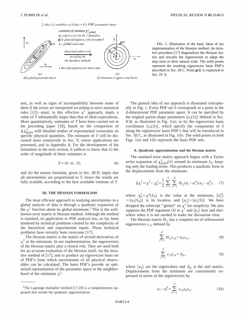
FIG. 1. Illustration of the basic ideas of ouimplementation of the Hessian method. An itertive procedure@17# diagonalizes the Hessian matrix and rescales the eigenvectors to adaptstep sizes to their natural scale. The solid poinrepresent the resulting eigenvector basis PDdescribed in Sec. III C. Pointp( i) is explained inSec. IV A.

oic

ns

fon

ath

atef

n

oeo

ic

oorora

sev-pb

tu-e

by

s

in

lor

in

r.al

x-

-

sets, as well as signs of incompatibility between somethem if the errors are interpreted according to strict statistrules @12#—must, in this effectivex2 approach, imply avalue ofT substantially larger than that of ideal expectatioMore quantitatively, estimates ofT have been carried out inthe preceding paper@18#, based on the comparison oDxglobal

2 with detailed studies of experimental constraintsspecific physical quantities. The estimates ofT will be dis-cussed more extensively in Sec. V, where applicationspresented, and in Appendix A. For the development offormalism in the next section, it suffices to know that~i! theorder of magnitude of these estimates is

T'10 to 15, ~6!

and ~ii ! the master formulas, given in Sec. III D, imply thall uncertainties are proportional toT, hence the results arfully scalable, according to the best available estimate oT.

III. THE HESSIAN FORMALISM

The most efficient approach to studying uncertainties iglobal analysis of data is through a quadratic expansionthe x2 function about its global minimum.2 This is the well-known error matrix or Hessian method. Although the methis standard, its application to PDF analysis has, so far, bhindered by technical problems created by the complexitythe theoretical and experimental inputs. Those technproblems have recently been overcome@17#.

The Hessian matrix is the matrix of second derivativesx2 at the minimum. In our implementation, the eigenvectof the Hessian matrix play a central role. They are used bfor an accurate evaluation of the Hessian itself, via the itetive method of@17#, and to produce an eigenvector basisof PDF’s from which uncertainties of all physical obserables can be calculated. The basis PDF’s provide an omized representation of the parameter space in the neighhood of the minimumx2.

2The Lagrange multiplier method@17,18# is a complementary approach that avoids the quadratic approximation.

01401

fal

.

ree

aof

denf

al

fsth-t

ti-or-

The general idea of our approach is illustrated concepally in Fig. 1. Every PDF setS corresponds to a point in thd-dimensional PDF parameter space. It can be specifiedthe original parton shape parameters$ai(S)% defined in Sec.II B, as illustrated in Fig. 1~a!; or by the eigenvector basicoordinates$zk(S)%, which specify the components ofSalong the eigenvector basis PDF’s that will be introducedSec. III C, as illustrated in Fig. 1~b!. The solid points in bothFigs. 1~a! and 1~b! represent the basis PDF sets.

A. Quadratic approximation and the Hessian matrix

The standard error matrix approach begins with a Tayseries expansion ofxglobal

2 (S) around its minimumS0, keep-ing only the leading terms. This produces a quadratic formthe displacements from the minimum:

Dx25x22x025

1

2 (i 51

d

(j 51

d

Hi j ~ai2ai0!~aj2aj

0!, ~7!

where x025x2(S0) is the value at the minimum,$aj

0%5$aj (S0)% is its location, and$aj%5$aj (S)%. We havedropped the subscript ‘‘global’’ onx2 for simplicity. We alsosuppress the PDF argument~S! in x2 and$ai% here and else-where when it is not needed to make the discussion clea

The Hessian matrixHi j has a complete set of orthonormeigenvectorsv ik defined by

(j 51

d

Hi j v jk5ekv ik , ~8!

(i 51

d

v i l v ik5d lk , ~9!

where $ek% are the eigenvalues andd lk is the unit matrix.Displacements from the minimum are conveniently epressed in terms of the eigenvectors by

ai2ai05 (

k51

d

v ikskzk , ~10!

3-4

w

er

.ofr

t

i-

th

n

toisr-glo-onbu-e

un-

ex-rs isd inw-

d

esveryif-lodsen

ap-eri-

a-

by-he

ente,t

ei-t tolef

n. 1:

the

ts


where scale factorssk are introduced to normalize the neparameterszk such that

Dx25 (k51

d

zk2 . ~11!

With this normalization, the relevant neighborhood~5! of theglobal minimum corresponds to the interior of a hypersphof radiusT:

(k51

d

zk2<T2. ~12!

The scale factorssk are approximately equal toA2/ek, as isexplained in Appendix B.

The transformation~10! is illustrated conceptually in Fig1, where$k,l % label two of the eigenvector directions. Onethe eigenvectorsvl is shown both in the original parametebasis and in the normalized eigenvector basis.

B. Eigenvalues of the Hessian matrix

The square of the distance in parameter space fromminimum of x2 is

(i 51

d

~ai2ai0!25 (

k51

d

~skzk!2 ~13!

by Eqs. ~9!, ~10!. Becausesk'A2/ek, an eigenvector withlarge eigenvalueek , therefore, corresponds to a ‘‘steep drection’’ in $ai% space, i.e., a direction in whichx2 risesrapidly, making the parameters tightly constrained bydata. The opposite is an eigenvector with smallek , whichcorresponds to a ‘‘shallow direction,’’ for which the criterioDx2<T2 permits considerable motion—as is the case forvlillustrated in Fig. 1.

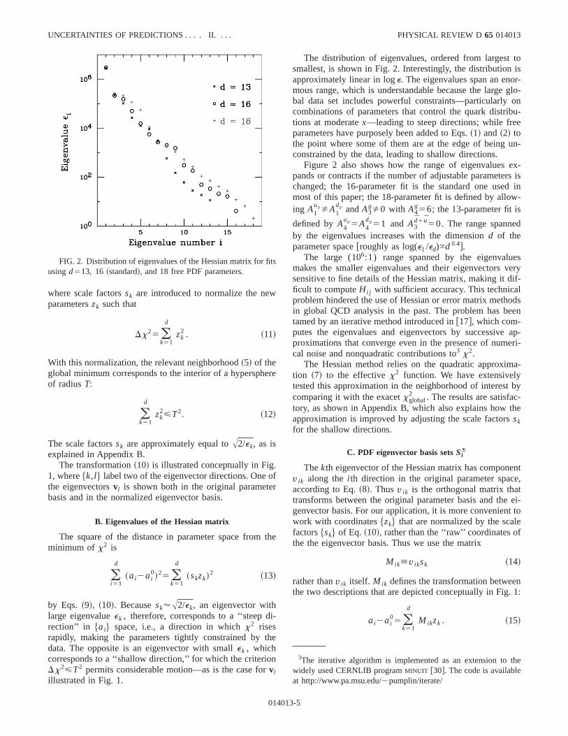
FIG. 2. Distribution of eigenvalues of the Hessian matrix for fiusingd513, 16~standard!, and 18 free PDF parameters.

01401

e

he

e

The distribution of eigenvalues, ordered from largestsmallest, is shown in Fig. 2. Interestingly, the distributionapproximately linear in loge. The eigenvalues span an enomous range, which is understandable because the largebal data set includes powerful constraints—particularlycombinations of parameters that control the quark distritions at moderatex—leading to steep directions; while freparameters have purposely been added to Eqs.~1! and~2! tothe point where some of them are at the edge of beingconstrained by the data, leading to shallow directions.

Figure 2 also shows how the range of eigenvaluespands or contracts if the number of adjustable parametechanged; the 16-parameter fit is the standard one usemost of this paper; the 18-parameter fit is defined by alloing A1

uvÞA1dv andA3

gÞ0 with A4g56; the 13-parameter fit is

defined byA4uv5A4

dv51 and A3d1u50. The range spanne

by the eigenvalues increases with the dimensiond of theparameter space@roughly as log(e1 /ed)}d 0.4#.

The large (106:1) range spanned by the eigenvalumakes the smaller eigenvalues and their eigenvectorssensitive to fine details of the Hessian matrix, making it dficult to computeHi j with sufficient accuracy. This technicaproblem hindered the use of Hessian or error matrix methin global QCD analysis in the past. The problem has betamed by an iterative method introduced in@17#, which com-putes the eigenvalues and eigenvectors by successiveproximations that converge even in the presence of numcal noise and nonquadratic contributions to3 x2.

The Hessian method relies on the quadratic approximtion ~7! to the effectivex2 function. We have extensivelytested this approximation in the neighborhood of interestcomparing it with the exacetxglobal

2 . The results are satisfactory, as shown in Appendix B, which also explains how tapproximation is improved by adjusting the scale factorsskfor the shallow directions.

C. PDF eigenvector basis setsSlÁ

Thekth eigenvector of the Hessian matrix has componv ik along thei th direction in the original parameter spacaccording to Eq.~8!. Thusv ik is the orthogonal matrix thatransforms between the original parameter basis and thegenvector basis. For our application, it is more convenienwork with coordinates$zk% that are normalized by the scafactors$sk% of Eq. ~10!, rather than the ‘‘raw’’ coordinates othe the eigenvector basis. Thus we use the matrix

Mik[v iksk ~14!

rather thanv ik itself. Mik defines the transformation betweethe two descriptions that are depicted conceptually in Fig

ai2ai05 (

k51

d

M ikzk . ~15!

3The iterative algorithm is implemented as an extension towidely used CERNLIB programMINUIT @30#. The code is availableat http://www.pa.msu.edu/;pumplin/iterate/

3-5

fittrihe

sao

e

an

-

cd

t-istiosi

se

the

a

It

atrs

. IV

ntial

m

cs.

he

celle

o


It contains information about the physics in the globaltogether with information related to the choice of paramezation, and is a good object to study for insight into how tparametrization might be improved, as we discuss in SIV A.

The eigenvectors provide an optimized orthonormal bain the PDF parameter space, which leads to a simple paretrization of the parton distributions in the neighborhoodthe global minimumS0. In the remainder of this section, wshow how to construct theseeigenvector basisPDF’s$Sl

6 ,l 51, . . . ,d%, and in the following section, we showhow they can be used to calculate the uncertainty ofchosen variableX(S).

The eigenvector basissetsSl6 are defined by displace

ments of a standard magnitudet ‘‘up’’ or ‘‘down’’ along eachof the d eigenvector directions. Their coordinates in thezbasis are thus

zk~Sl6!56tdkl . ~16!

More explicitly, S11 is defined by (z1 , . . . ,zd)

5(t,0, . . . ,0), etc. We make displacements in both diretions along each eigenvector to improve accuracy; whichrection is called ‘‘up’’ is totally arbitrary. As a practical mater, we chooset55 for the displacement distance. Thchoice improves the accuracy of the quadratic approximaby working with displacements that have about the sameas those needed in applications.4

The$ai% parameters that specify the eigenvector basisSl

6 are given by

ai~Sl6!2ai

056tM il , ~17!

by Eqs.~15!, ~16!. Hence

ai~Sl1!2ai~Sl

2!52tM il . ~18!

Interpreted as a difference equation, this shows directlythe elementMil of the transformation matrix is equal to thgradient of parameterai along the direction of5 zl .

Basis PDF sets along two of the eigenvector directionsillustrated conceptually in Figs. 1~a! and 1~b! as solid pointsdisplaced from the global minimum setS0. The coefficientsthat specify all of the setsSl

6 are listed in Table IV of Ap-pendix D.

4The value chosen fort is somewhat smaller than the typicalTgiven in Eq.~6! because in applications, the component of displament along a given eigenvector direction will generally be smathan the total displacement.

5Technically, we calculate the orthogonal matrixv i j using dis-placements that giveDx2.5, where the iterative procedure@17#converges well. The eigenvectors are then scaled up by an amthat is adjusted to makeDx2525 exactly for eachSk

6 to improvethe quadratic approximation.

01401

,-ec.

ism-f

y

-i-

nze

ts

at

re

D. Master equations for calculating uncertainties using theeigenvector basis setsSl

Á‰

Let X(S) be any variable that depends on the PDF’s.can be a physical quantity such as theW production crosssection; or a particular PDF such as the gluon distributionspecificx andQ values; or even one of the PDF parameteai . All of these cases will be used as examples in Secsand V.

The best-fit estimate forX is X05X(S0). To find the un-certainty, it is only necessary to evaluateX for each of the 2dsets$Sl

6%. The gradient ofX in the z representation can thebe calculated, using a linear approximation that is essento the Hessian method, by

]X

]zk5

X~Sk1!2X~Sk

2!

2t, ~19!

where t is the scale used to define$Sl6% in Eq. ~16!. It is

useful to define

Dk~X!5X~Sk1!2X~Sk

2!, ~20!

D~X!5S (k51

d

@Dk~X!#2D 1/2

, ~21!

Dk~X!5Dk~X!/D~X!, ~22!

so thatDk(X) is a vector in the gradient direction andDk(X)is the unit vector in that direction.

The gradient direction is the direction in whichX variesmost rapidly, so the largest variations inX permitted by Eq.~12! are obtained by displacement from the global minimuS0 in the gradient direction by a distance6T. Hence

DX5 (k51

d

~TDk!]X

]zk. ~23!

From this, using Eqs.~19!–~22!, we obtain themaster equa-tion for calculating uncertainties,

DX5T

2tD~X!. ~24!

This equation is applied to obtain numerical results in SeIV and V.

For applications, it is often important to also construct tPDF setsSX

1 and SX2 that achieve the extreme valuesX

5X06DX. Their z coordinates are

zk~SX6!56TDk~X!, ~25!

which follows from the derivation of Eq.~24!. Their physicalparameters$ai% then follow from Eqs.~15! and ~18!:

ai~SX6!2ai

056T

2t (k51

d

Dk~X!@ai~Sk1!2ai~Sk

2!#. ~26!

-r

unt

3-6

i-

e


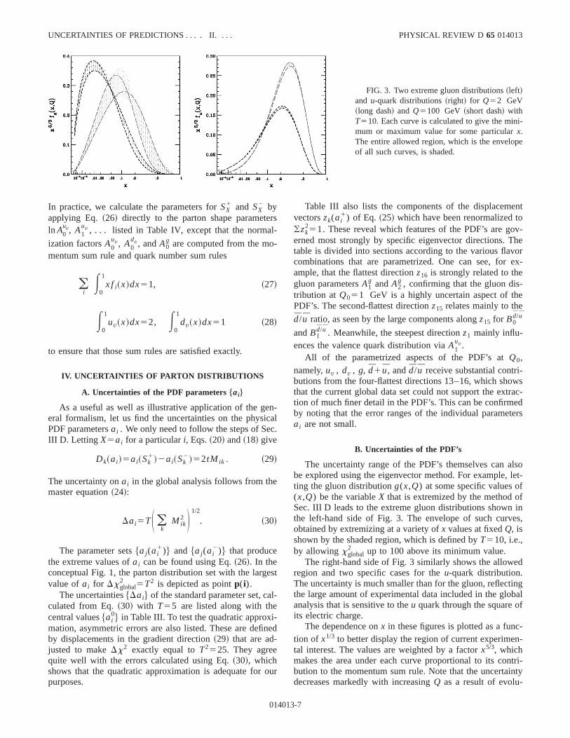
FIG. 3. Two extreme gluon distributions~left!and u-quark distributions~right! for Q52 GeV~long dash! and Q5100 GeV ~short dash! withT510. Each curve is calculated to give the minmum or maximum value for some particularx.The entire allowed region, which is the envelopof all such curves, is shaded.

rsl-

-

ncac.

es

l-

i-n

o

entoov-he

vorex-

e

-wsrac-eders

lsolet-ffin

es,

d

ingbalf

c-n-

ntri-nty

In practice, we calculate the parameters forSX1 and SX

2 byapplying Eq. ~26! directly to the parton shape parameteln A0

uv, A1uv , . . . listed in Table IV, except that the norma

ization factorsA0uv, A0

dv, andA0g are computed from the mo

mentum sum rule and quark number sum rules

(iE

0

1

x f i~x!dx51, ~27!

E0

1

uv~x!dx52, E0

1

dv~x!dx51 ~28!

to ensure that those sum rules are satisfied exactly.

IV. UNCERTAINTIES OF PARTON DISTRIBUTIONS

A. Uncertainties of the PDF parametersˆai‰

As a useful as well as illustrative application of the geeral formalism, let us find the uncertainties on the physiPDF parametersai . We only need to follow the steps of SeIII D. Letting X5ai for a particulari, Eqs.~20! and~18! give

Dk~ai !5ai~Sk1!2ai~Sk

2!52tM ik . ~29!

The uncertainty onai in the global analysis follows from themaster equation~24!:

Dai5TS (k

M ik2 D 1/2

. ~30!

The parameter sets$aj (ai1)% and $aj (ai

2)% that producethe extreme values ofai can be found using Eq.~26!. In theconceptual Fig. 1, the parton distribution set with the largvalue ofai for Dxglobal

2 5T2 is depicted as pointp( i).The uncertainties$Dai% of the standard parameter set, ca

culated from Eq.~30! with T55 are listed along with thecentral values$ai

0% in Table III. To test the quadratic approxmation, asymmetric errors are also listed. These are defiby displacements in the gradient direction~29! that are ad-justed to makeDx2 exactly equal toT2525. They agreequite well with the errors calculated using Eq.~30!, whichshows that the quadratic approximation is adequate forpurposes.

01401

-l

t

ed

ur

Table III also lists the components of the displacemvectorszk(ai

1) of Eq. ~25! which have been renormalized t(zk

251. These reveal which features of the PDF’s are gerned most strongly by specific eigenvector directions. Ttable is divided into sections according to the various flacombinations that are parametrized. One can see, forample, that the flattest directionz16 is strongly related to thegluon parametersA1

g andA2g , confirming that the gluon dis-

tribution at Q051 GeV is a highly uncertain aspect of thPDF’s. The second-flattest directionz15 relates mainly to the

d/u ratio, as seen by the large components alongz15 for B0d/u

andB1d/u . Meanwhile, the steepest directionz1 mainly influ-

ences the valence quark distribution viaA1uv.

All of the parametrized aspects of the PDF’s atQ0,namely,uv , dv , g, d1u, andd/u receive substantial contributions from the four-flattest directions 13–16, which shothat the current global data set could not support the exttion of much finer detail in the PDF’s. This can be confirmby noting that the error ranges of the individual parametai are not small.

B. Uncertainties of the PDF’s

The uncertainty range of the PDF’s themselves can abe explored using the eigenvector method. For example,ting the gluon distributiong(x,Q) at some specific values o(x,Q) be the variableX that is extremized by the method oSec. III D leads to the extreme gluon distributions shownthe left-hand side of Fig. 3. The envelope of such curvobtained by extremizing at a variety ofx values at fixedQ, isshown by the shaded region, which is defined byT510, i.e.,by allowing xglobal

2 up to 100 above its minimum value.The right-hand side of Fig. 3 similarly shows the allowe

region and two specific cases for theu-quark distribution.The uncertainty is much smaller than for the gluon, reflectthe large amount of experimental data included in the gloanalysis that is sensitive to theu quark through the square oits electric charge.

The dependence onx in these figures is plotted as a funtion of x1/3 to better display the region of current experimetal interest. The values are weighted by a factorx5/3, whichmakes the area under each curve proportional to its cobution to the momentum sum rule. Note that the uncertaidecreases markedly with increasingQ as a result of evolu-

3-7


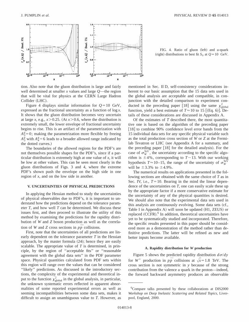
FIG. 4. Ratio of gluon~left! and u-quark~right! distributions to best fitS0 at Q510 GeV.

ly

n

gai

ntitngb

arpa

thmon

tien

rashiri-a-

in

y

leetthre-in,noa

es

in-d inon-n-

.a-perthech

d

o-

fol-

-pfor

ed.d in

eore,sid-de-d

,ble

000

tion. Also note that the gluon distribution is large and fairwell determined at smallerx values and largeQ—the regionthat will be vital for physics at the CERN Large HadroCollider ~LHC!.

Figure 4 displays similar information forQ510 GeV,expressed as the fractional uncertainty as a function of lox.It shows that the gluon distribution becomes very uncertat largex, e.g.,x.0.25.~At x.0.6, where the distribution isextremely small, the lower envelope of fractional uncertaibegins to rise. This is an artifact of the parametrization wA3

g50; making the parametrization more flexible by freeiA3

g with A4g56 leads to a broader allowed range indicated

the dotted curves.!The boundaries of the allowed regions for the PDF’s

not themselves possible shapes for the PDF’s, since if aticular distribution is extremely high at one value ofx, it willbe low at other values. This can be seen most clearly ingluon distributions of Figs. 3 and 4, where the extrePDF’s shown push the envelope on the high side inregion ofx, and on the low side in another.

V. UNCERTAINTIES OF PHYSICAL PREDICTIONS

In applying the Hessian method to study the uncertainof physical observables due to PDF’s, it is important to uderstand how the predictions depend on the tolerance paeterT, and how wellT can be determined. We discuss theissues first, and then proceed to illustrate the utility of tmethod by examining the predictions for the rapidity distbution of W andZ boson production as well as the correltion of W andZ cross sections inpp collisions.

First, note that the uncertainties of all predictions are learly dependent on the tolerance parameterT in the Hessianapproach, by the master formula~24!; hence they are easilscalable. The appropriate value ofT is determined, in prin-ciple, by the region of ‘‘acceptable fits’’ or ‘‘reasonabagreement with the global data sets’’ in the PDF paramspace. Physical quantities calculated from PDF sets withis region will range over the values that can be conside‘‘likely’’ predictions. As discussed in the introductory sections, the complexity of the experimental and theoreticalput to the functionxglobal

2 in the global analysis, in particularthe unknown systematic errors reflected in apparent abmalities of some reported experimental errors as wellseeming incompatibilities between some data sets, makdifficult to assign an unambiguous value toT. However, as

01401

n

yh

y

er-

eee

s-m-es

-

erind

-

r-sit

mentioned in Sec. II D, self-consistency considerationsherent to our basic assumption that the 15 data sets usethe global analysis are acceptable and compatible, in cjunction with the detailed comparison to experiment coducted in the preceding paper@18# using the samexglobal

2

function, yield a best estimate ofT'10 to 15@~Eq. 6!#. De-tails of these considerations are discussed in Appendix A

Of the estimates ofT described there, the most quantittive one is based on the algorithm of the preceding pa@18# to combine 90% confidence level error bands from15 individual data sets for any specific physical variable suas the total production cross section ofW or Z at the Fermi-lab Tevatron or LHC~see Appendix A for a summary, anthe preceding paper@18# for the detailed analysis!. For thecase ofsW

TeV , the uncertainty according to the specific algrithm is 64%, corresponding toT;13. With our workinghypothesisT'10–15, the range of the uncertainty ofsW

TeV

will be 63.3% to64.9%.The numerical results on applications presented in the

lowing sections are obtained with the same choice ofT as inSec. IV, i.e.,T510. Bearing in the mind the linear dependence of the uncertainties onT, one can easily scale these uby the appropriate factor if a more conservative estimatethe uncertainty of any of the physical quantities is desirWe should also note that the experimental data sets usethis analysis are continuously evolving. Some data sets~cf.,Table I in Appendix A! will soon be updated~H1, ZEUS! orreplaced~CCFR!.6 In addition, theoretical uncertainties havyet to be systematically studied and incorporated. Therefthe specific results presented in this paper should be conered more as a demonstration of the method rather thanfinitive predictions. The latter will be refined as new anbetter inputs become available.

A. Rapidity distribution for W production

Figure 5 shows the predicted rapidity distributionds/dy

for W1 production in pp collisions atAs51.8 TeV. Thecross section is not symmetric iny because of the strongcontribution from the valenceu quark in the proton—indeedthe forward backward asymmetry produces an observa

6Compare talks presented by these collaborations at DIS2Workshop on Deep Inelastic Scattering and Related Topics, Liver-pool, England, 2000.

3-8

ss

w


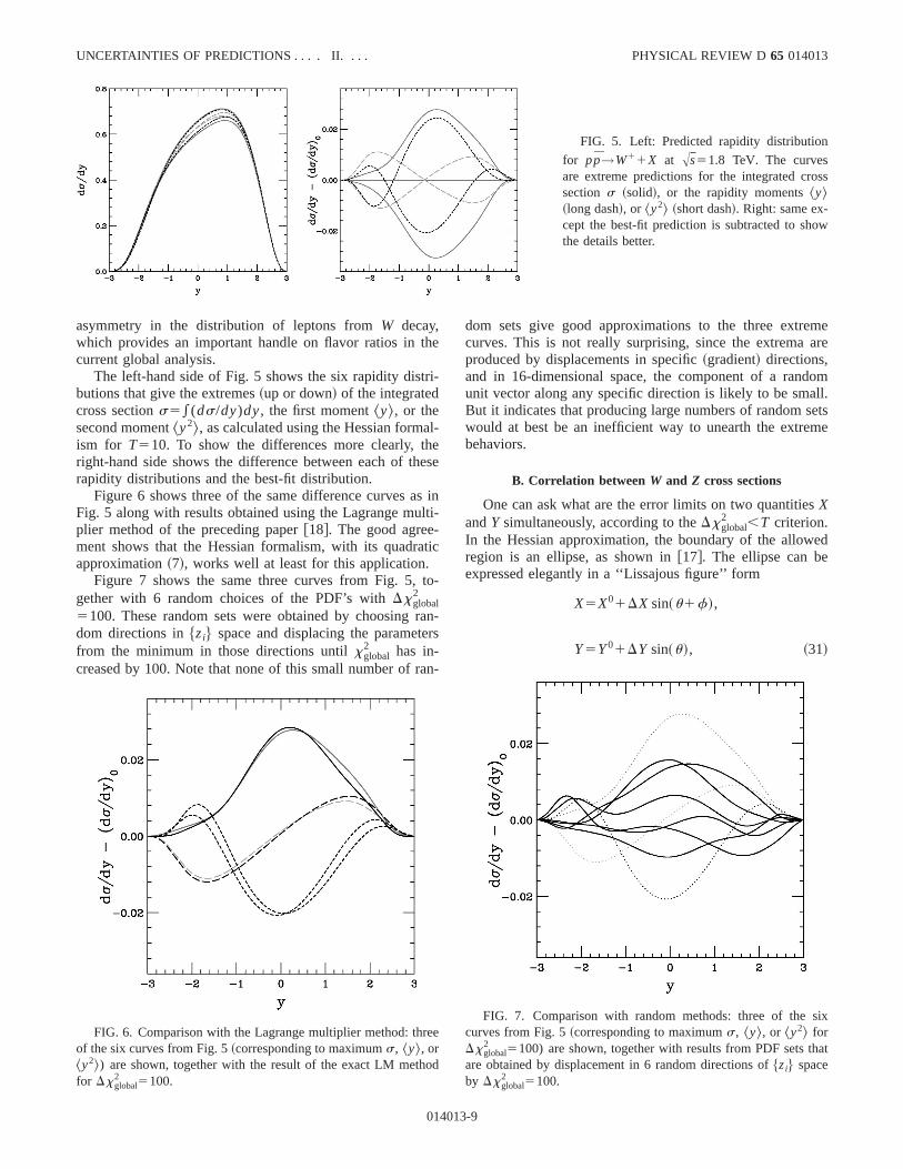
FIG. 5. Left: Predicted rapidity distribution

for pp→W11X at As51.8 TeV. The curvesare extreme predictions for the integrated crosection s ~solid!, or the rapidity momentsy&~long dash!, or ^y2& ~short dash!. Right: same ex-cept the best-fit prediction is subtracted to shothe details better.

he

ri-

alhee

slt

t

to

rar

a

meare

omll.etsme

ed

ee

od

six

hat

asymmetry in the distribution of leptons fromW decay,which provides an important handle on flavor ratios in tcurrent global analysis.

The left-hand side of Fig. 5 shows the six rapidity distbutions that give the extremes~up or down! of the integratedcross sections5*(ds/dy)dy, the first moment y&, or thesecond momenty2&, as calculated using the Hessian formism for T510. To show the differences more clearly, tright-hand side shows the difference between each of thrapidity distributions and the best-fit distribution.

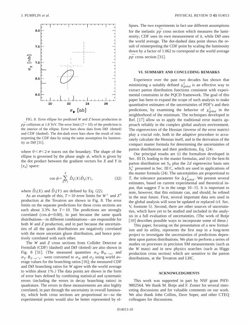
Figure 6 shows three of the same difference curves aFig. 5 along with results obtained using the Lagrange muplier method of the preceding paper@18#. The good agree-ment shows that the Hessian formalism, with its quadraapproximation~7!, works well at least for this application.

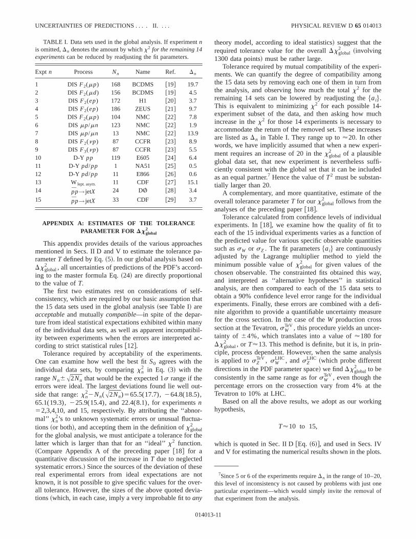
Figure 7 shows the same three curves from Fig. 5,gether with 6 random choices of the PDF’s withDxglobal

2

5100. These random sets were obtained by choosingdom directions in$zi% space and displacing the parametefrom the minimum in those directions untilxglobal

2 has in-creased by 100. Note that none of this small number of r

FIG. 6. Comparison with the Lagrange multiplier method: throf the six curves from Fig. 5~corresponding to maximums, ^y&, or^y2&) are shown, together with the result of the exact LM methfor Dxglobal

2 5100.

01401

-

se

ini-

ic

-

n-s

n-

dom sets give good approximations to the three extrecurves. This is not really surprising, since the extremaproduced by displacements in specific~gradient! directions,and in 16-dimensional space, the component of a randunit vector along any specific direction is likely to be smaBut it indicates that producing large numbers of random swould at best be an inefficient way to unearth the extrebehaviors.

B. Correlation betweenW and Z cross sections

One can ask what are the error limits on two quantitiesXandY simultaneously, according to theDxglobal

2 ,T criterion.In the Hessian approximation, the boundary of the allowregion is an ellipse, as shown in@17#. The ellipse can beexpressed elegantly in a ‘‘Lissajous figure’’ form

X5X01DX sin~u1f!,

Y5Y01DY sin~u!, ~31!

FIG. 7. Comparison with random methods: three of thecurves from Fig. 5~corresponding to maximums, ^y&, or ^y2& forDxglobal

2 5100) are shown, together with results from PDF sets tare obtained by displacement in 6 random directions of$zi% spaceby Dxglobal

2 5100.

3-9

h

roa

yrk

foin

tes

at

emat

igs

the

ons

i-esre-

ityge

that

ri-his

akeeir

in-nt.

cu-theof

sof

oll in-onedd in

in-ly-

e.al-rmen-s of

n

Y-er-ork.EQ

inno


where 0,u,2p traces out the boundary. The shape of tellipse is governed by the phase anglef, which is given bythe dot product between the gradient vectors forX andY in$zk% space:

cosf5 (k51

d

Dk~X!Dk~Y!, ~32!

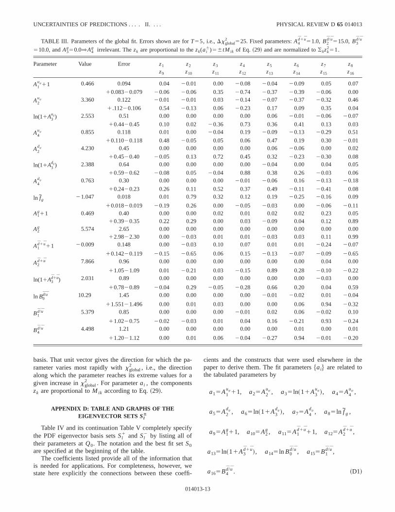
whereD i(X) and D i(Y) are defined by Eq.~22!.As an example of this,T510 error limits forW6 andZ0

production at the Tevatron are shown in Fig. 8. The erlimits on the separate predictions for these cross sectionseach about 3.3% forT510. The predictions are stronglcorrelated (cosf50.60), in part because the same quadistributions—in different combinations—are responsibleboth W andZ production, and in part because the uncertaties of all the quark distributions are negatively correlawith the more uncertain gluon distribution, and hence potively correlated with each other.

The W and Z cross sections from Collider DetectorFermilab~CDF! ~dashed! and DØ~dotted! are also shown inFig. 8 @31#. ~The measured quantitiessW•BW→en andsZ•BZ→e1e2 were converted tosW andsZ using world av-erage values for the branching ratios@16#; the measured CDFand DØ branching ratios forW agree with the world averagto within about 1%.! The data points are shown in the forof error bars defined by combining statistical and systemerrors ~including the errors in decay branching ratios! inquadrature. The errors in these measurements are also hcorrelated, in part through the uncertainty in overall luminoity, which both cross sections are proportional to—soexperimental points would also be better represented by

FIG. 8. Error ellipse for predictedW andZ boson production in

pp collisions at 1.8 TeV. The error limit (T510) of the prediction isthe interior of the ellipse. Error bars show data from DØ~dotted!and CDF~dashed!. The dot-dash error bars show the result of reterpreting the CDF data by using the same assumption for lumiity as DØ @31#.

01401

e

rre

r-di-

ic

hly-el-

lipses. The two experiments in fact use different assumpti

for the inelasticpp cross section which measures the lumnosity; CDF uses its own measurement of it, while DØ usthe world average. The dot-dashed data point shows thesult of reinterpreting the CDF point by scaling the luminosdown by a factor of 1.062 to correspond to the world avera

pp cross section@31#.

VI. SUMMARY AND CONCLUDING REMARKS

Experience over the past two decades has shownminimizing a suitably definedxglobal

2 is an effective way toextract parton distribution functions consistent with expemental constraints in the PQCD framework. The goal of tpaper has been to expand the scope of such analysis to mquantitative estimates of the uncertainties of PDF’s and thpredictions, by examining the behavior ofxglobal

2 in theneighborhood of the minimum. The techniques developedRef. @17# allow us to apply the traditional error matrix approach reliably in the complex global analysis environmeThe eigenvectors of the Hessian~inverse of the error matrix!play a crucial role, both in the adaptive procedure to acrately calculate the Hessian itself, and in the derivation ofcompact master formula for determining the uncertaintiesparton distributions and their predictions, Eq.~24!.

Our principal results are~i! the formalism developed inSec. III D, leading to the master formulas, and~ii ! the best-fitparton distribution setS0 plus the 2d eigenvector basis setSk

6 presented in Sec. III C, which are used in applicationsthe master formula~24!. The uncertainties are proportional tT, the tolerance parameter forDxglobal

2 . We present severaestimates, based on current experimental and theoreticaput, that suggestT is in the range 10–15. It is important tnote, however, that this estimate can, and should, be refiin the near future. First, several important data sets usethe global analysis will soon be updated or replaced~cf. Sec.V, footnote 5!. Second, there are other sources of uncertaties, which have yet to be studied and included in the anasis in a full evaluation of uncertainties.~The work of Botje@10# describes possible ways to incorporate some of thes!

This paper, focusing on the presentation of a new formism and its utility, represents the first step in a long-teproject to investigate the uncertainties of predictions depdent upon parton distributions. We plan to perform a seriestudies on processes in precision SM measurements~such asthe W mass! and in new physics searches~such as Higgsproduction cross section! which are sensitive to the partodistributions, at the Tevatron and LHC.

ACKNOWLEDGMENTS

This work was supported in part by NSF grant PH9802564. We thank M. Botje and F. Zomer for several intesting discussions and for valuable comments on our wWe also thank John Collins, Dave Soper, and other CTcolleagues for discussions.

-s-

3-10

hepnd

elth

niba

ts

ut

ra

th

senoervi

ri-ngom

uchtoases

eri-

uffi-ed

-

the

al

ofties

he

ay,calts toualefi-ure

r-

-lysis

the

ing

ts.

neof

t


APPENDIX A: ESTIMATES OF THE TOLERANCEPARAMETER FOR Dxglobal

2

This appendix provides details of the various approacmentioned in Secs. II D and V to estimate the tolerancerameterT defined by Eq.~5!. In our global analysis based oDxglobal

2 , all uncertainties of predictions of the PDF’s accoring to the master formula Eq.~24! are directly proportionalto the value ofT.

The first two estimates rest on considerations of sconsistency, which are required by our basic assumptionthe 15 data sets used in the global analysis~see Table I! areacceptableand mutuallycompatible—in spite of the depar-ture from ideal statistical expectations exhibited within maof the individual data sets, as well as apparent incompatity between experiments when the errors are interpretedcording to strict statistical rules@12#.

Tolerance required by acceptability of the experimenOne can examine how well the best fitS0 agrees with theindividual data sets, by comparingxn

2 in Eq. ~3! with therangeNn6A2Nn that would be the expected 1s range if theerrors were ideal. The largest deviations found lie well oside that range:xn

22Nn(A2Nn)565.5(17.7),264.8(18.5),65.1(19.3),225.9(15.4), and 22.4(8.1), for experimentsn52,3,4,10, and 15, respectively. By attributing the ‘‘abnomal’’ xn

2’s to unknown systematic errors or unusual fluctutions ~or both!, and accepting them in the definition ofxglobal

2

for the global analysis, we must anticipate a tolerance forlatter which is larger than that for an ‘‘ideal’’x2 function.~Compare Appendix A of the preceding paper@18# for aquantitative discussion of the increase inT due to neglectedsystematic errors.! Since the sources of the deviation of thereal experimental errors from ideal expectations areknown, it is not possible to give specific values for the ovall tolerance. However, the sizes of the above quoted detions~which, in each case, imply a very improbable fit toany

TABLE I. Data sets used in the global analysis. If experimennis omitted,Dn denotes the amount by whichx2 for the remaining 14experimentscan be reduced by readjusting the fit parameters.

Expt n Process Nn Name Ref. Dn

1 DIS F2(mp) 168 BCDMS @19# 19.72 DIS F2(md) 156 BCDMS @19# 4.53 DIS F2(ep) 172 H1 @20# 3.74 DIS F2(ep) 186 ZEUS @21# 9.75 DIS F2(mp) 104 NMC @22# 7.86 DIS mp/mn 123 NMC @22# 1.97 DIS mp/mn 13 NMC @22# 13.98 DIS F2(np) 87 CCFR @23# 8.99 DIS F3(np) 87 CCFR @23# 5.510 D-Y pp 119 E605 @24# 6.411 D-Y pd/pp 1 NA51 @25# 0.512 D-Y pd/pp 11 E866 @26# 0.613 Wlept. asym. 11 CDF @27# 15.114 pp→ jetX 24 DO” @28# 3.4

15 pp→ jetX 33 CDF @29# 3.7

01401

sa-

-

f-at

yil-c-

.

-

--

e

t-a-

theory model, according to ideal statistics! suggest that therequired tolerance value for the overallDxglobal

2 ~involving1300 data points! must be rather large.

Tolerance required by mutual compatibility of the expements. We can quantify the degree of compatibility amothe 15 data sets by removing each one of them in turn frthe analysis, and observing how much the totalx2 for theremaining 14 sets can be lowered by readjusting the$ai%.This is equivalent to minimizingx2 for each possible 14-experiment subset of the data, and then asking how mincrease in thex2 for those 14 experiments is necessaryaccommodate the return of the removed set. These increare listed asDn in Table I. They range up to'20. In otherwords, we have implicitly assumed that when a new expment requires an increase of 20 in thexglobal

2 of a plausibleglobal data set, that new experiment is nevertheless sciently consistent with the global set that it can be includas an equal partner.7 Hence the value ofT2 must be substantially larger than 20.

A complementary, and more quantitative, estimate ofoverall tolerance parameterT for our xglobal

2 follows from theanalyses of the preceding paper@18#.

Tolerance calculated from confidence levels of individuexperiments. In@18#, we examine how the quality of fit toeach of the 15 individual experiments varies as a functionthe predicted value for various specific observable quantisuch assW or sZ . The fit parameters$ai% are continuouslyadjusted by the Lagrange multiplier method to yield tminimum possible value ofxglobal

2 for given values of thechosen observable. The constrainted fits obtained this wand interpreted as ‘‘alternative hypotheses’’ in statistianalysis, are then compared to each of the 15 data seobtain a 90% confidence level error range for the individexperiments. Finally, these errors are combined with a dnite algorithm to provide a quantifiable uncertainty measfor the cross section. In the case of theW production crosssection at the Tevatron,sW

TeV , this procedure yields an uncetainty of 64%, which translates into a value of'180 forDxglobal

2 , or T'13. This method is definite, but it is, in principle, process dependent. However, when the same anais applied tosZ

TeV , sWLHC , andsZ

LHC ~which probe differentdirections in the PDF parameter space! we findDxglobal

2 to beconsistently in the same range as forsW

TeV , even though thepercentage errors on the crossection vary from 4% atTevatron to 10% at LHC.

Based on all the above results, we adopt as our workhypothesis,

T'10 to 15,

which is quoted in Sec. II D@Eq. ~6!#, and used in Secs. IVand V for estimating the numerical results shown in the plo

7Since 5 or 6 of the experiments requireDn in the range of 10–20,this level of inconsistency is not caused by problems with just oparticular experiment—which would simply invite the removalthat experiment from the analysis.

3-11

cellyc

eeu

DF1

th

-u

pret

tiodhentin

irbi

im

esine

ly

e

ap

est

e

heio

n-by

romesum-ate,

-ept-


Finally, it is of some interest to compare this toleranestimate with the traditional—although by now generarecognized as questionable—gauge provided by differenbetween published PDF’s.

Comparison of tolerance figures to differences betwpublished PDF’s. Table II lists the value obtained when oxglobal

2 is computed using various current and historical Psets. TheDx2 column lists the increase over the CTEQ5Mset. Typical values for the modern sets are similar torange 100–225 that corresponds toT510–15. For previousgenerations of PDF sets,xglobal

2 is much larger—not surprisingly, because the obsolete sets were extracted from mless accurate data, and without some of the physicalcesses such asW decay lepton asymmetry and inclusive jproduction.

APPENDIX B: TESTS OF THE QUADRATICAPPROXIMATION

The Hessian method relies on a quadratic approxima~7! to the effectivex2 function in the relevant neighborhooof its minimum. To test this approximation, Fig. 9 shows tdependence ofx2 along a representative sample of the eigevector directions. The steep directions 1 and 4 are indisguishable from the ideal quadratic curveDx25z2. The shal-lower directions 7, 10, 13, and 16, are represented fawell by that parabola, although they exhibit noticeable cuand higher-order effects. The agreement at smallz is notperfect because we adjust the scale factorssk in Eq. ~10! ~seefootnote 5! to improve the average agreement over theportant regionz&5, rather than defining the matrixHi j inEq. ~7! strictly by the second derivatives atz50. For thisreason, the scale factorssk in Eq. ~17! are somewhat differ-ent from theA2/ek suggested by the Taylor series: the flattdirections are extremely flat only over very small intervalsz, so it would be misleading to represent them solely by thcurvature atz50.

Figure 10 shows the dependence ofx2 along some ran-dom directions in$zi% space. The behavior is reasonabclose to the ideal quadratic curveDx25z2, implying that thequadratic approximation~7! is adequate. In particular, thapproximation gives the range ofz permitted byT510 to anaccuracy of'30%. Since the tolerance parameterT used tomake the uncertainty estimates is known only to perh50%, this level of accuracy is sufficient.

TABLE II. Overall xglobal2 values and their increments above t

best-fit value, for some current and historical parton distributsets.

Current sets x2 Dx2 Historical sets x2 Dx2

CTEQ5M1 1188 - CTEQ4M 1540 352CTEQ5HJ 1272 84 MRSR2 1680 492MRST99 1297 109 MRSR1 1758 570MRST-a↓ 1356 168 CTEQ3M 2254 1066MRST-a↑ 1531 343 MRSA’ 3371 2183

01401

es

nr

e

cho-

n

--

lyc

-

t

ir

s

APPENDIX C: TABLE OF BEST FIT S0

Table III lists the parameter values that define the ‘‘bfit’’ PDF set S0, which minimizesxglobal

2 . It also lists theuncertainties~for T55) in those parameters.

For each of thed516 parameters, Table III also lists thcomponents of a unit vectorz1 , . . . ,zd in the eigenvector

n

FIG. 9. Variation ofx2 with distance along representative eigevector directions 1, 4, 7, 10, 13, and 16. The first two, shownsolid curves, are nearly indistinguishable from each other and fthe idealDx25z2. The remaining four, shown by dashed curvwith increasing dash length denoting increasing eigenvector nber, demonstrate that the quadratic approximation is adequthough imperfect.

FIG. 10. Variation ofx2 with distance along 10 randomly chosen directions in$zi% space. The dependence is represented accably well by the quadratic approximationDx25z2, which is shownas the dotted curve.

3-12

5

0

0

1


TABLE III. Parameters of the global fit. Errors shown are forT55, i.e.,Dxglobal2 525. Fixed parameters:A4

d1u51.0, B2d/u515.0, B3

d/u

510.0, andA3g50.0⇒A4

g irrelevant. Thezk are proportional to thezk(ai6)56tM ik of Eq. ~29! and are normalized to(kzk

251.

Parameter Value Error z1 z2 z3 z4 z5 z6 z7 z8

z9 z10 z11 z12 z13 z14 z15 z16

A1uv11 0.466 0.094 0.04 20.01 0.00 20.08 20.04 20.09 0.05 0.07

10.08320.079 20.06 20.06 0.35 20.74 20.37 20.39 20.06 0.00

A2uv 3.360 0.122 20.01 20.01 0.03 20.14 20.07 20.37 20.32 0.46

1.11220.106 0.54 20.13 0.06 20.23 0.17 0.09 0.35 0.04

ln(11A3uv) 2.553 0.51 0.00 0.00 0.00 0.00 0.06 20.01 20.06 20.07

10.4420.45 0.10 0.02 20.36 0.73 0.36 0.41 0.13 0.03

A4uv 0.855 0.118 0.01 0.00 20.04 0.19 20.09 20.13 20.29 0.51

10.11020.118 0.48 20.05 0.05 0.06 0.47 0.19 0.30 20.01

A2dv 4.230 0.45 0.00 0.00 0.00 0.00 0.06 20.06 0.00 0.02

10.4520.40 20.05 0.13 0.72 0.45 0.32 20.23 20.30 0.08

ln(11A3dv) 2.388 0.64 0.00 0.00 0.00 0.00 20.04 0.00 0.04 0.05

10.5920.62 20.08 0.05 20.04 0.88 0.38 0.26 20.03 0.06

A4dv 0.763 0.30 0.00 0.00 0.00 20.01 20.06 0.16 20.13 20.18

10.2420.23 0.26 0.11 0.52 0.37 0.49 20.11 20.41 0.08

ln fg21.047 0.018 0.01 0.79 0.32 0.12 0.19 20.25 20.16 0.09

10.01820.019 20.19 0.26 0.00 20.05 20.03 0.00 20.06 20.11A1

g11 0.469 0.40 0.00 0.00 0.02 0.01 0.02 0.02 0.23 0.010.3920.35 0.22 0.29 0.00 0.03 20.09 0.04 0.12 0.89

A2g 5.574 2.65 0.00 0.00 0.00 0.00 0.00 0.00 0.00 0.0

12.9822.30 0.00 20.03 0.01 0.01 20.03 0.03 0.11 0.99

A1d1u11 20.009 0.148 0.00 20.03 0.10 0.07 0.01 0.01 20.24 20.07

10.14220.119 20.15 20.65 0.06 0.15 20.13 20.07 20.09 20.65

A2d1u 7.866 0.96 0.00 0.00 0.00 0.00 0.00 0.00 0.04 0.0

11.0521.09 0.01 20.21 0.03 20.15 0.89 0.28 20.10 20.22

ln(11A3d1u) 2.031 0.89 0.00 0.00 0.00 0.00 0.00 0.00 20.03 0.00

10.7820.89 20.04 0.29 20.05 20.28 0.66 0.20 0.04 0.59

ln B0d/u 10.29 1.45 0.00 0.00 0.00 0.00 20.01 20.02 0.01 20.04

11.55121.496 0.00 0.01 0.03 0.00 0.00 0.06 0.94 20.32

B1d/u 5.379 0.85 0.00 0.00 0.00 20.01 0.02 0.06 20.02 0.10

11.0220.75 20.02 20.03 0.01 0.04 0.16 20.21 0.93 20.24

B4d/u 4.498 1.21 0.00 0.00 0.00 0.00 0.00 0.01 0.00 0.0

11.2021.12 0.00 0.01 0.06 20.04 20.27 0.94 20.01 20.20

a

or

ify

atw

ef

the
basis. That unit vector gives the direction for which the prameter varies most rapidly withxglobal
2 , i.e., the directionalong which the parameter reaches its extreme values fgiven increase inxglobal

2 . For parameterai , the componentszk are proportional toMik according to Eq.~29!.

APPENDIX D: TABLE AND GRAPHS OF THEEIGENVECTOR SETS Sl

Á

Table IV and its continuation Table V completely specthe PDF eigenvector basis setsSl

1 and Sl2 by listing all of

their parameters atQ0. The notation and the best fit setS0are specified at the beginning of the table.

The coefficients listed provide all of the information this needed for applications. For completeness, however,state here explicitly the connections between these co

01401

-

a

efi-

cients and the constructs that were used elsewhere inpaper to derive them. The fit parameters$ai% are related tothe tabulated parameters by

a15A1uv11, a25A2

uv , a35 ln~11A3uv!, a45A4

uv ,

a55A2dv , a65 ln~11A3

dv!, a75A4dv , a85 ln f g ,

a95A1g11, a105A2

g , a115A1d1u11, a125A2

d1u ,

a135 ln~11A3d1u!, a145 ln B0

d/u , a155B1d/u ,

a165B4d/u . ~D1!

3-13

4980

4980

4980

4990

4949

4863

5031

4814


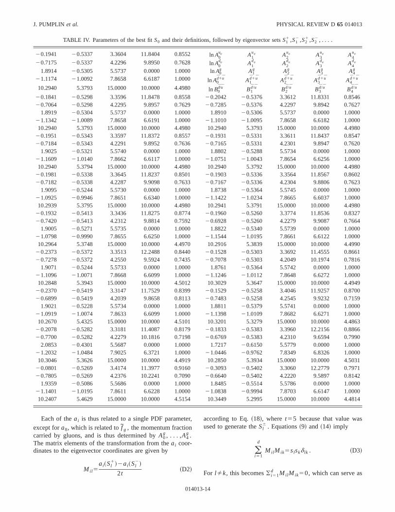
TABLE IV. Parameters of the best fitS0 and their definitions, followed by eigenvector setsS11 ,S1

2 ,S21 ,S2

2 , . . . .

20.1941 20.5337 3.3604 11.8404 0.8552 ln A0uv A1

uv A2uv A3

uv A4uv

20.7175 20.5337 4.2296 9.8950 0.7628 ln A0dv A1

dv A2dv A3

dv A4dv

1.8914 20.5305 5.5737 0.0000 1.0000 ln A0g A1

g A2g A3

g A4g

21.1174 21.0092 7.8658 6.6187 1.0000 ln A0d1u A1

d1u A2d1u A3

d1u A4d1u

10.2940 5.3793 15.0000 10.0000 4.4980 ln B0d/u B1

d/u B2d/u B3

d/u B4d/u

20.1841 20.5298 3.3596 11.8478 0.8558 20.2042 20.5376 3.3612 11.8331 0.854620.7064 20.5298 4.2295 9.8957 0.7629 20.7285 20.5376 4.2297 9.8942 0.7627

1.8919 20.5304 5.5737 0.0000 1.0000 1.8910 20.5306 5.5737 0.0000 1.000021.1342 21.0089 7.8658 6.6191 1.0000 21.1010 21.0095 7.8658 6.6182 1.000010.2940 5.3793 15.0000 10.0000 4.4980 10.2940 5.3793 15.0000 10.0000 4.

20.1951 20.5343 3.3597 11.8372 0.8557 20.1931 20.5331 3.3611 11.8437 0.854720.7184 20.5343 4.2291 9.8952 0.7636 20.7165 20.5331 4.2301 9.8947 0.7620

1.9025 20.5321 5.5740 0.0000 1.0000 1.8802 20.5288 5.5734 0.0000 1.000021.1609 21.0140 7.8662 6.6117 1.0000 21.0751 21.0043 7.8654 6.6256 1.000010.2940 5.3794 15.0000 10.0000 4.4980 10.2940 5.3792 15.0000 10.0000 4.

20.1981 20.5338 3.3645 11.8237 0.8501 20.1903 20.5336 3.3564 11.8567 0.860220.7182 20.5338 4.2287 9.9098 0.7633 20.7167 20.5336 4.2304 9.8806 0.7623

1.9095 20.5244 5.5730 0.0000 1.0000 1.8738 20.5364 5.5745 0.0000 1.000021.0925 20.9946 7.8651 6.6340 1.0000 21.1422 21.0234 7.8665 6.6037 1.000010.2939 5.3795 15.0000 10.0000 4.4980 10.2941 5.3791 15.0000 10.0000 4.

20.1932 20.5413 3.3436 11.8275 0.8774 20.1960 20.5260 3.3774 11.8536 0.832720.7420 20.5413 4.2312 9.8814 0.7592 20.6928 20.5260 4.2279 9.9087 0.7664

1.9005 20.5271 5.5735 0.0000 1.0000 1.8822 20.5340 5.5739 0.0000 1.000021.0798 20.9990 7.8655 6.6250 1.0000 21.1544 21.0195 7.8661 6.6122 1.000010.2964 5.3748 15.0000 10.0000 4.4970 10.2916 5.3839 15.0000 10.0000 4.

20.2373 20.5372 3.3513 12.2488 0.8440 20.1528 20.5303 3.3692 11.4555 0.866120.7278 20.5372 4.2550 9.5924 0.7435 20.7078 20.5303 4.2049 10.1974 0.7816

1.9071 20.5244 5.5733 0.0000 1.0000 1.8761 20.5364 5.5742 0.0000 1.000021.1096 21.0071 7.8668 6.6099 1.0000 21.1246 21.0112 7.8648 6.6272 1.000010.2848 5.3943 15.0000 10.0000 4.5012 10.3029 5.3647 15.0000 10.0000 4.

20.2370 20.5419 3.3147 11.7529 0.8399 20.1529 20.5258 3.4046 11.9257 0.870020.6899 20.5419 4.2039 9.8658 0.8113 20.7483 20.5258 4.2545 9.9232 0.7159

1.9021 20.5228 5.5734 0.0000 1.0000 1.8811 20.5379 5.5741 0.0000 1.000021.0919 21.0074 7.8633 6.6099 1.0000 21.1398 21.0109 7.8682 6.6271 1.000010.2670 5.4325 15.0000 10.0000 4.5101 10.3201 5.3279 15.0000 10.0000 4.

20.2078 20.5282 3.3181 11.4087 0.8179 20.1833 20.5383 3.3960 12.2156 0.886620.7700 20.5282 4.2279 10.1816 0.7198 20.6769 20.5383 4.2310 9.6594 0.7990

2.0853 20.4301 5.5687 0.0000 1.0000 1.7217 20.6150 5.5779 0.0000 1.000021.2032 21.0484 7.9025 6.3721 1.0000 21.0446 20.9762 7.8349 6.8326 1.000010.3046 5.3626 15.0000 10.0000 4.4919 10.2850 5.3934 15.0000 10.0000 4.

20.0801 20.5269 3.4174 11.3977 0.9160 20.3093 20.5402 3.3060 12.2779 0.797120.7805 20.5269 4.2376 10.2241 0.7090 20.6640 20.5402 4.2220 9.5897 0.8142

1.9359 20.5086 5.5686 0.0000 1.0000 1.8485 20.5514 5.5786 0.0000 1.000021.1401 21.0195 7.8611 6.6228 1.0000 21.0838 20.9994 7.8703 6.6147 1.000010.2407 5.4629 15.0000 10.0000 4.5154 10.3449 5.2995 15.0000 10.0000 4.

er s
Each of theai is thus related to a single PDF parametexcept fora8, which is related tof g , the momentum fractioncarried by gluons, and is thus determined byA0
g , . . . ,A4g .

The matrix elements of the transformation from theai coor-dinates to the eigenvector coordinates are given by

Mil 5ai~Sl

1!2ai~Sl2!

2t~D2!

01401

,according to Eq.~18!, where t55 because that value waused to generate theSl

6 . Equations~9! and ~14! imply

(i 51

d

M il M ik5slskd lk . ~D3!

For lÞk, this becomes( i 51d Mil M ik50, which can serve as

3-14

3

2

0

0

.5031

6

6

0

0

.4910

1

8

0

0

.4309

7

5

0

0

.5518

2

3

0

0

.8382

0

6

0

0

.3936

7

5

0

0

.5039

6

1

0

0

.7094


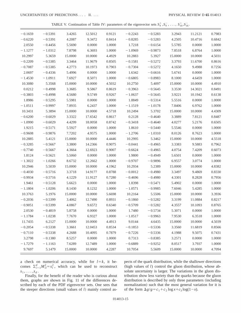
TABLE V. Continuation of Table IV: parameters of the eigenvector setsS91 ,S9

2 , . . . , S161 ,S16

2 .

20.1659 20.5391 3.4265 12.5012 0.9121 20.2243 20.5283 3.2943 11.2121 0.798

20.6220 20.5391 4.2087 9.3472 0.8414 20.8285 20.5283 4.2505 10.4716 0.684

2.0550 20.4456 5.5690 0.0000 1.0000 1.7218 20.6154 5.5785 0.0000 1.000

21.1277 21.0312 7.8798 6.3693 1.0000 21.0969 20.9873 7.8518 6.8764 1.000

10.2997 5.3659 15.0000 10.0000 4.4929 10.2883 5.3927 15.0000 10.0000 4

20.2209 20.5385 3.3464 11.9679 0.8505 20.1581 20.5272 3.3793 11.6700 0.861

20.7087 20.5385 4.2773 10.1973 0.7903 20.7304 20.5272 4.1650 9.4988 0.725

2.0697 20.4336 5.4996 0.0000 1.0000 1.6342 20.6616 5.6741 0.0000 1.000

21.4530 21.0911 7.6927 8.5071 1.0000 20.6805 20.8983 8.1000 4.6459 1.000

10.3080 5.3568 15.0000 10.0000 4.5032 10.2750 5.4097 15.0000 10.0000 4

0.0212 20.4998 3.3685 9.5867 0.8619 20.3963 20.5645 3.3530 14.3021 0.849

20.3803 20.4998 4.5680 9.5749 0.9267 21.0637 20.5645 3.9221 10.1942 0.613

1.8986 20.5295 5.5981 0.0000 1.0000 1.8849 20.5314 5.5516 0.0000 1.000

21.0511 20.9997 7.8935 6.2437 1.0000 21.1519 21.0178 7.8406 6.9762 1.000

10.3431 5.3894 15.0000 10.0000 4.5718 10.2494 5.3702 15.0000 10.0000 4

20.6200 20.6029 3.3322 17.6542 0.8617 0.2128 20.4640 3.3889 7.8121 0.848

21.0990 20.6029 4.4299 18.0058 0.8742 20.3418 20.4640 4.0277 5.2176 0.650

1.9215 20.5171 5.5927 0.0000 1.0000 1.8610 20.5440 5.5546 0.0000 1.000

20.9608 20.9876 7.7202 4.9575 1.0000 21.2706 21.0310 8.0126 8.7623 1.000

10.2885 5.4121 15.0000 10.0000 4.4446 10.2995 5.3462 15.0000 10.0000 4

20.3285 20.5667 3.3800 14.2366 0.9075 20.0441 20.4965 3.3383 9.5883 0.796

20.7740 20.5667 4.3664 12.6923 0.9007 20.6624 20.4965 4.0754 7.4209 0.607

1.8124 20.5621 5.5060 0.0000 1.0000 1.9800 20.4949 5.6501 0.0000 1.000

21.3022 21.0266 8.6732 12.2662 1.0000 20.9707 20.9896 6.9557 3.0774 1.000

10.2946 5.5039 15.0000 10.0000 4.1962 10.2934 5.2389 15.0000 10.0000 4

20.4030 20.5716 3.3718 14.9177 0.8788 20.0012 20.4980 3.3497 9.4869 0.833

20.9934 20.5716 4.1229 11.9127 0.7280 20.4696 20.4980 4.3301 8.2828 0.795

1.9461 20.5128 5.6623 0.0000 1.0000 1.8398 20.5471 5.4902 0.0000 1.000

21.1804 21.0206 8.1430 8.1232 1.0000 21.0571 20.9985 7.6046 5.4285 1.000

10.3763 5.1976 15.0000 10.0000 5.6698 10.2164 5.5506 15.0000 10.0000 3

20.2036 20.5399 3.4062 12.7490 0.8931 20.1860 20.5282 3.3199 11.0884 0.821

20.9051 20.5399 4.0867 9.6572 0.6340 20.5709 20.5282 4.3557 10.1093 0.876

2.0530 20.4819 5.8758 0.0000 1.0000 1.7480 20.5734 5.3071 0.0000 1.000

21.1784 21.0238 7.7670 6.9327 1.0000 21.0517 20.9963 7.9530 6.3518 1.000

11.7435 6.2127 15.0000 10.0000 4.4913 9.0144 4.6435 15.0000 10.0000 4

20.2054 20.5338 3.3661 12.0453 0.8534 20.1853 20.5336 3.3560 11.6819 0.856

20.7110 20.5338 4.2688 10.4095 0.7879 20.7226 20.5336 4.1988 9.5075 0.743

3.2798 20.1380 8.5257 0.0000 1.0000 0.7313 20.8385 3.2571 0.0000 1.000

21.7279 21.1163 7.6289 12.7489 1.0000 20.6889 20.9252 8.0517 3.7937 1.000

9.7697 5.1479 15.0000 10.0000 4.2287 10.7054 5.5609 15.0000 10.0000 4

ct

udet

ns-is-

luon

is

a check on numerical accuracy, while forl 5k, it be-comes ( i 51

d Mil2 5sl

2 , which can be used to reconstrus1 , . . . ,sd .

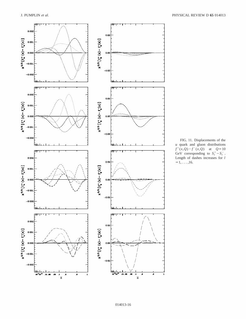
Finally, for the benefit of the reader who is curious abothem, graphs are shown in Fig. 11 of the differencesscribed by each of the PDF eigenvector sets. One seesthe steeper directions~small values ofl ! mainly control as-

01401

t-

hat

pects of the quark distribution, while the shallower directio~high values ofl ) control the gluon distribution, whose absolute uncertainty is larger. The variations in the gluon dtribution show less variety than the quarks because the gdistribution is described by only three parameters~includingnormalization! such that the most general variation for itof the formDg/g5c11c2 logx1c3 log(12x).

3-15


FIG. 11. Displacements of theu quark and gluon distributionsf 1(x,Q)2 f 2(x,Q) at Q510GeV corresponding toSl

12Sl2 .

Length of dashes increases forl51, . . .,16.

014013-16

.F

ur

ur

.E

nd.

p:d

l.

p

o-

ev.

lk,

1

cs

va-a-


@1# H.L. Lai, J. Huston, S. Kuhlmann, J. Morfin, F. Olness, JOwens, J. Pumplin, and W.K. Tung, Eur. Phys. J. C12, 375~2000!.

@2# A.D. Martin, R.G. Roberts, W.J. Stirling, and R.S. Thorne, EPhys. J. C4, 463 ~1998!.

@3# M. Gluck, E. Reya, and A. Vogt, Eur. Phys. J. C5, 461~1998!.@4# James Bottset al., Phys. Lett. B304, 159 ~1993!; H.L. Lai

et al., Phys. Rev. D51, 4763~1995!; 55, 1280~1997!.@5# A.D. Martin, R.G. Roberts, W.J. Stirling, and R.S. Thorne, E

Phys. J. C14, 133 ~2000!.@6# J. Huston, S. Kuhlmann, H.L. Lai, F. Olness, J.F. Owens, D

Soper, and W.K. Tung, Phys. Rev. D58, 114034~1998!.@7# Contributions to the Proceedings of the Workshop, ‘‘QCD a

Weak Boson Physics in Run II,’’ Batavia, Illinois, edited by UBaur, R.K. Ellis, and D. Zeppenfeld, Fermilab Pub-00/297.

@8# S. Cataniet al., The QCD and standard model working grouSummary Report, LHC Workshop ‘‘Standard Model anMore,’’ CERN, 1999, hep-ph/0005114.

@9# S. Alekhin, Eur. Phys. J. C10, 395 ~1999!; contribution toProceedings of Standard Model Physics~and more! at the LHC@8#; S.I. Alekhin, Phys. Rev. D63, 094022~2001!.

@10# M. Botje, Eur. Phys. J. C14, 285 ~2000!.@11# V. Barone, C. Pascaud, and F. Zomer, Eur. Phys. J. C12, 243

~2000!; C. Pascaud and F. Zomer, LAL-95-05.@12# W.T. Giele and S. Keller, Phys. Rev. D58, 094023~1998!; D.

Kosower, talk given at ‘‘Les Rencontres de Physique deValle d’Aoste,’’ La Thuile, 1999; W.T. Giele, S. Keller, and DKosower, in Ref.@7#.

@13# R. Brock, D. Casey, J. Huston, J. Kalk, J. Pumplin, D. Stumand W.K. Tung, in Ref.@7#.

@14# W. Bialek, C.G. Callan, and S.P. Strong, Phys. Rev. Lett.77,4693 ~1996!; V. Periwal, Phys. Rev. D59, 094006~1999!.

@15# R.D. Ball, in Proceedings of the XXXIVth Rencontres de Mriond, QCD and Hadronic Interactions, Les Arcs, 1999.

@16# Particle Data Group, D. Groomet al., Eur. Phys. J. C15, 1~2000!.

01401

.

.

.

.

a

,

@17# J. Pumplin, D.R. Stump, and W.K. Tung, this issue, Phys. RD 65, 014011~2002!.

@18# D. Stump, J. Pumplin, R. Brock, D. Casey, J. Huston, J. KaH. L. Lai, and W.K. Tung, preceeding paper, Phys. Rev. D65,014012~2002!.

@19# BCDMS Collaboration, A.C. Benvenutiet al., Phys. Lett. B223, 485 ~1989!; 237, 592 ~1990!.

@20# H1 Collaboration, S. Aidet al., Nucl. Phys.B439, 471~1995!;‘‘1994 data,’’ DESY-96-039, hep-ex/9603004 and HWebpage.

@21# ZEUS Collaboration, M. Derricket al., Z. Phys. C65, 379~1995!; ‘‘1994 data,’’ DESY-96-076, 1996.

@22# NMC Collaboration, M. Arneodoet al., Phys. Lett. B364, 107~1995!.

@23# CCFR Collaboration, W.C. Leunget al., Phys. Lett. B317,655 ~1993!; P.Z. Quintaset al., Phys. Rev. Lett.71, 1307~1993!.

@24# E605 Collaboration, G. Morenoet al., Phys. Rev. D43, 2815~1991!.

@25# NA51 Collaboration, A. Balditet al., Phys. Lett. B332, 244~1994!.

@26# E866 Collaboration, E.A. Hawkeret al., Phys. Rev. Lett.80,3715 ~1998!.

@27# CDF Collaboration, F. Abeet al., Phys. Rev. Lett.74, 850~1995!.

@28# D0 Collaboration, B. Abbottet al., Phys. Rev. Lett.82, 2451~1999!; hep-ex/9807018.

@29# CDF Collaboration, F. Abeet al., Phys. Rev. Lett.77, 438~1996!; F. Bedeschi, talk at 1999 Hadron Collider PhysiConference, Bombay, 1999.

@30# F. James and M. Roos, Comput. Phys. Commun.10, 343~1975!; Minuit manual, http://wwwinfo.cern.ch/asdoc/minuit/

@31# F. Lehner, ‘‘Some aspects of W / Z boson physics at the Tetron,’’ in Proceedings of 4th Rencontres du Vietnam: Interntional Conference on Physics at Extreme Energies~ParticlePhysics and Astrophysics!, Hanoi, Vietnam, 2000,FERMILAB-CONF-00-273-E, 2000.

3-17

uncertainties of predictions from parton distribution

Documents