two-layer baroclinic eddy heat fluxes: zonal flows and energy

Two-Layer Baroclinic Eddy Heat Fluxes: Zonal Flows and Energy Balance

ANDREW F. THOMPSON AND WILLIAM R. YOUNG

Scripps Institution of Oceanography, University of California, San Diego, La Jolla, California

(Manuscript received 27 September 2006, in final form 13 December 2006)

ABSTRACT

The eddy heat flux generated by statistically equilibrated baroclinic turbulence supported on a uniform,horizontal temperature gradient is examined using a two-layer �-plane quasigeostrophic model. The de-pendence of the eddy diffusivity of temperature, D�, on external parameters such as �, bottom friction �,the deformation radius �, and the velocity jump 2U, is provided by numerical simulations at 110 differentpoints in the parameter space �* � ��2/U and �* � ��/U. There is a special “pivot” value of �*, �piv

* �11/16, at which D� depends weakly on �*. But otherwise D� has a complicated dependence on both �* and�*, highlighted by the fact that reducing �* leads to increases (decreases) in D� if � is less than (greater than)�piv

* . Existing heat-flux parameterizations, based on Kolmogorov cascade theories, predict that D� is non-zero and independent of �* in the limit �* → 0. Simulations show indications of this regime provided that�* � 0.04 and 0.25 � �* � 0.5.

All important length scales in this problem, namely the mixing length, the scale of the energy containingeddies, the Rhines scale, and the spacing of the zonal jets, converge to a common value as bottom frictionis reduced. The mixing length and jet spacing do not decouple in the parameter regime considered here, aspredicted by cascade theories. The convergence of these length scales is due to the formation of jet-scaleeddies that align along the eastward jets. The baroclinic component of these eddies helps force the zonalmean flow, which occurs through nonzero Reynolds stress correlations in the upper layer, as opposed to thebarotropic mode. This behavior suggests that the dynamics of the inverse barotropic cascade are insufficientto fully describe baroclinic turbulence.

1. Introduction

Rhines (1977) and Salmon (1980) characterize en-ergy transfers in baroclinic turbulence as a direct cas-cade of the baroclinic mode and a simultaneous inversecascade of the barotropic mode. This dual cascade sce-nario serves as an interpretive framework for recentparameterizations of meridional eddy heat and poten-tial vorticity fluxes (Larichev and Held 1995; Held andLarichev 1996; Lapeyre and Held 2003). In these theo-ries, the barotropic inverse cascade proceeds to smallwavenumbers until the cascade halts at a wavenumberk0. The length k�1

0 characterizes the largest barotropiceddies and k�1

0 is also the mixing length of heat andpotential vorticity. There are two mechanisms thatmight determine k0 by slowing or halting the inverse

cascade: the planetary potential vorticity gradient, �,and bottom friction.

Because the � effect does not dissipate energy, �alone cannot halt the inverse cascade and determine k0.Thus, bottom drag plays an essential role at the termi-nus of the inverse cascade by dissipating the kineticenergy continually supplied by the release of availablepotential energy. In other words, truly halting the in-verse cascade requires dissipation at large scales, andonly bottom drag can accomplish this. An extreme casethat makes this point is the problem of statisticallysteady baroclinic turbulence with � � 0. At this � � 0end point, the eddy heat flux is exponentially sensitiveto the strength of the bottom drag coefficient (Thomp-son and Young 2006).

In view of the importance of bottom drag, it is dis-maying that the bottom drag coefficient does not playan explicit role in the heat-flux parameterizations pro-posed by Held and Larichev (1996) and Lapeyre andHeld (2003, hereafter LH03). A defense of these drag-less heat-flux parameterizations relies on the ability of� to direct energy into zonal flows (Rhines 1975; Wil-

Corresponding author address: Andrew F. Thompson, School ofEnvironmental Sciences, University of East Anglia, Norwich NR47TJ, United Kingdom.E-mail: [email protected]

3214 J O U R N A L O F T H E A T M O S P H E R I C S C I E N C E S VOLUME 64

DOI: 10.1175/JAS4000.1

© 2007 American Meteorological Society

JAS4000

liams 1979; Panetta 1993; Vallis and Maltrud 1993; Lee1997). Zonal flows do not contribute to meridionaleddy diffusion and therefore do not release availablepotential energy. In this view, the strong zonal flowsspontaneously generated by baroclinic turbulence, seeFigs. 1, 2, serve as a nondiffusive reservoir of barotropickinetic energy and, through bottom friction, as the en-ergy sink at the terminal wavenumber of the inversecascade (Smith et al. 2002). Thus it is possible to main-tain, following LH03, that with � � 0 the amplitude ofeddy heat fluxes is insensitive to the bottom drag coef-ficient.

This seems too good to be true, and throughout mostof the parameter space it is: a main goal in this compu-tational study of baroclinic instability is to document

the importance of bottom drag in limiting barocliniceddy heat fluxes. We consider the combined effects of� and bottom friction on meridional eddy heat fluxesand report results based on a suite of 110 statisticallyequilibrated simulations of baroclinic turbulence.These simulations significantly extend and augment theparameter regimes of previous studies. Although thedependence on bottom drag is not nearly as strong asthe exponential relation found by Thompson andYoung (2006) in the � � 0 limit, the new simulationsshow that, even with substantial �, bottom drag remainsan important control parameter.

In section 2 we introduce the energy balance integraland define the eddy diffusivities that are used to sum-marize the suite of simulations. In section 3 we review

FIG. 1. (a) Growth rates of the linear baroclinic instability for three values of �* ��/U, all with �* ��/U � 0.02;bottom friction produces instability at the frictionless critical value �* � 1. (b) Three time series of the eddy diffusivityD� /U� all at �* � 0.02. The “instantaneous” diffusivity is defined by taking the angle brackets in (1) only as an (x, y)average. (c) Hovmöller diagram of the zonally averaged barotropic velocity �y with �* � 0.5, �* � 0.02. (d) Snapshotof the eddy streamfunction � � � for the simulation in (c); � is dominated by isotropic eddies with the same scaleas the zonal jets in (c). (e), (f) As in (c), (d) but for a simulation with �* � 1 and �* � 0.02.

SEPTEMBER 2007 T H O M P S O N A N D Y O U N G 3215

and assess the LH03 theory of baroclinic eddy fluxes. Insection 4 we survey the important length scales in theproblem (the mixing length, the scale of the energycontaining eddies, the Rhines scale, and the spacing ofthe zonal jets) and show that, when the bottom drag issufficiently weak, all length scales converge to a com-mon value. We also show that large, jet-scale eddiesmake the dominant contribution to the eddy heat fluxand force the zonal mean flow through upper-layer (notbarotropic) Reynolds stresses. In section 5 we confirmthat eddy diffusivities and heat fluxes are insensitive tothe domain scale L and to the hyperdiffusivity. Our

conclusions are presented in section 6. The equations ofmotion are summarized in the appendix.

2. Eddy fluxes and diffusivities

To summarize the results of our simulations, we cal-culate an eddy diffusivity of temperature, D�, and ob-tain the dependence of D� on external parameters suchas the domain size L, the bottom drag coefficient �, theRossby deformation radius �, the imposed velocityjump 2U, and �. Our notation is introduced systemati-cally in the appendix and is largely the same as that of

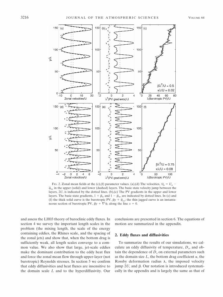
FIG. 2. Zonal mean fields at the (c),(f) parameter values. (a),(d) The velocities, Un � Un �ny in the upper (solid) and lower (dashed) layers. The basic state velocity jump between thelayers, 2U, is indicated by the dotted lines. (b),(e) The PV gradients in the upper and lowerlayers. The basic state gradients, 1 � �* and 1 � �*, are indicated by dotted lines. In (c) and(f) the thick solid curve is the barotropic PV, �y � yy; the thin jagged curve is an instanta-neous section of barotropic PV, �y � 2, along the line x � 0.


Larichev and Held (1995): �(x, y, t) and (x, y, t) are thedisturbance streamfunctions of the baroclinic and baro-tropic modes, respectively. The baroclinic streamfunc-tion � plays the role of an interface displacement or athermal field. The large-scale gradient of the baroclinicmode is �U, and thus a precise definition of the eddydiffusivity of temperature, D�, is

D� U�1��x��. �1�

Here angle brackets denote both a horizontal averageover the square 2�L � 2�L domain and an additionaltime average to remove residual turbulent fluctuations.An important point is that D� is useful only if it isinsensitive to the domain size L (Haidvogel and Held1980). In this case one can hope that D� inferred froma spatially homogeneous calculation can be employedin a more realistic flow with scale separation between aslowly varying mean and baroclinic eddies (Pavan andHeld 1996).

The quantity �x�� in (1) is the product of the baro-tropic meridional velocity, x, and the thermal field � ;that is, the meridional heat flux is proportional to �x��.Moreover, the mechanical energy balance in a statisti-cally steady state (see the appendix) is

U��2��x�� |�� 2�� |2� � hyp�, �2�

where “hyp�” indicates the hyperviscous dissipation ofenergy. The first term on the right-hand side of (2) isthe mechanical energy dissipation (watts per kilogram)by bottom drag, �. We will refer to dissipation by bot-tom friction as

� �� |�� 2�� |2�, �3�

which neglects the hyperviscous contribution in (2).The left-hand side of (2) is the energy extracted fromthe unstable horizontal temperature gradient by baro-clinic instability. Enstrophy budgets also identify �x��as the large-scale source balancing the hyperviscous en-strophy sink at high wavenumbers.

As an alternative to the baroclinic–barotropic de-composition, the system can be represented in terms oftwo layers; the layerwise velocities and potential vor-ticities are defined in terms of and � in the appendix.The domain-averaged PV fluxes in the upper and lowerlayers are linearly related to the eddy heat flux by theTaylor–Bretherton relationship:

��1q1� � ��2q2� � ��2��x��. �4�

The basic state gradients of upper and lower layer PVare � � U��2 and � � U��2, respectively. Thus the

upper (n � 1) and lower (n � 2) layer PV diffusivitiesare related to D� by

D� � D1�1 ��2

U �, �5�

D� � D2�1 ��2

U � . �6�

Thus a single quantity, conveniently defined as D� in(1), summarizes all of the important quadratic powerintegrals and fluxes in homogeneous baroclinic turbu-lence.

Dimensional considerations (Haidvogel and Held1980) show that

D� � U� � D�*�L

�,��

U,��2

U,

UL7�, �7�

where D�* is a dimensionless function. The final argu-ment of D�*, involving the hyperviscosity �, is relativelysmall (see section 5). For brevity we suppress any ref-erence to this hyperviscous parameter. We also focuson a single value L/� � 25; however, we check fordependence on L as described in section 5.

Figure 3a summarizes a suite of 110 numerical simu-lations revealing the main features of the functionD�*(25, �*, �*), where �* ��2/U and �* ��/U.Here D�* varies over five orders of magnitude in re-sponse to much smaller changes in �* and �*. Sometrends in Fig. 3 are clear: D�* decreases monotonicallywith increasing �*. However, other dependences aremore complicated, particularly those related to bottomdrag. Close to the special “pivot” value �* � �piv

* �11/16, D�* has a weak dependence on bottom friction.For �* � �piv

* increasing bottom friction reduces D�*,whereas for �* � �piv

* increasing bottom friction in-creases D�*. This behavior is shown in Fig. 3b, whichillustrates the �* variation of D� at five values of �*.The same trends are evident in Fig. 14 of Panetta(1993).

Thompson and Young (2006) discuss the limitingcase �* � 0 in detail. Their conclusion is that a well-defined D�—independent of domain size—exists pro-vided that �* is not too small. The �* � 0 points in Fig.3 satisfy this condition and are in Thompson andYoung’s local mixing regime. However, this constraintmeans that the weakly damped runs with �* � 0.08cannot be extended to values of � less than about 0.25:to go below � � 0.25 and �* � 0.08 requires increasingthe domain size, so the largest eddies are smaller thanthe domain.

Notice that Fig. 3 shows nonzero diffusivities when�* 1. This is because bottom friction destabilizes thesystem beyond the frictionless critical value �* � 1


(Holopainen 1961; Pedlosky 1987; Arbic and Flierl2004). Consequently statistically steady, small nonzerovalues of D� are achievable out to at least �* � 1.5.

To summarize the results in Fig. 3 it is useful to havea compact formula for D�* in terms of �* and �*. Theempirical formula

D�* � �*�4�1.7 � �3 � 4�*��*�

�4, �8�

provided 0.25 � �* � 1.25, fits D�* to within �10%over a broad range of �* and �* values (see Fig. 4). Thedotted curve in Fig. 3 is D�* � 0.12��4

* , which is ob-tained from (8) by setting �* � 0. The fit (8) still has theproblem that D�* grows to infinity as �* → 0. At smallvalues of �*, a different expression tending toward theexponential dependence on �* observed by Thompsonand Young (2006) is required.

3. Review and assessment of LH03

The energy balance in (2) provides one relationshipbetween the dissipation � and the energy production or,equivalently, the eddy diffusivity D�. Specifically, using

the definitions of D� and � in (1) and (3) and neglectingthe hyperviscous dissipation we obtain

U2

�2 D� � �. �9�

Figure 5a shows that (9) is an excellent approximation;the small deviation of the ratio ��2/U2D� from 1 is dueto the hyp� contribution to the dissipation. The hyper-viscous dissipation is never more than 12% and can bereduced further by increasing the resolution (see sec-tion 5).

Held and Larichev (1996) propose a closure obtainedfrom cascade arguments in which � halts the barotropicinverse cascade by directing energy into zonal modes.Forming a diffusivity from � and the inverse cascaderate (which is assumed to be equivalent to � in a steadystate), dimensional analysis gives D� � c�3/5��4/5,where c is a dimensionless constant. This relation be-tween D, �, and � is supported by the arguments andnumerical simulations of Smith et al. (2002), which em-ploy a barotropic model. Combining D� � c�3/5��4/5

with (9) gives the Held and Larichev (1996) result,namely D� � c5/2U3/(�3�2).

FIG. 3. (a) Survey of the nondimensional meridional eddy heat flux D�/U� at 110 differentvalues of the parameters �* and �*. The dashed curve indicates the D� parameterization in(11) (with c � 1.65). The dotted line is an empirical fit 0.12��4

* . At �pivot � 0.72, there is weakdependence on �*. (b) Data at five values of �* (indicated by the dotted lines) are expandedto illustrate the weaker but still significant dependence on �*. The point at �* � 0.25 and�* � 0.02 is flagged with a “?” to indicate possible dependence on domain size (see section 5).


a. Selection of the lower-layer diffusivity

An immediate problem is that there are three diffu-sivities: in addition to D� we have the PV diffusivitiesD1 and D2 in (5) and (6). If one of these three diffu-sivities involves only � and �, then the other two willhave additional dependence on other parameters. Thusthe association of the dimensional combination c�3/5

��4/5 with D�, as opposed to D1 or D2, is a significanthypothesis. Indeed, LH03 updated the theory of Heldand Larichev (1996) by identifying the eddy diffusivityc�3/5��4/5 with the lower-layer PV diffusivity D2 ratherthan D�:

D2 � c�3�5��4�5. �10�

The motivation for (10) is that the weaker PV gradientin the lower layer allows larger meridional particle ex-cursions so that lower-layer PV behaves more like apassive tracer. The ratio ��4/5�3/5D�1

2 is shown in Fig.5b and there is strong and systematic dependence onboth � and �. However, the ratio is almost constant forthe runs with 0.25 � �* � 0.5 and �* � 0.08, and it is inthis corner of the parameter space that the theoreticalarguments of LH03 might apply. This region is dis-cussed in greater detail below.

Using (6) and (9), D2 and � are eliminated from (10),which yields the main prediction of LH03:

D� �U� � c5�2�*�2�1 � �*�

5�2, �11�

FIG. 4. The ratio of the lhs of (8) to the rhs.

FIG. 5. (a) Ratio of terms in the energy balance approximation U 2D� /�2 � �. The systematic departurefrom 1 is because the hyperviscous dissipation is not included in definition of � in (3). (b) The ratioD2 � �3/5��4/5.


where �* ��2/U. The relation above is the dashedcurve in Fig. 3 with c � 1.65.1

b. The rampant barotropic mode

An important assumption in the LH03 heat flux clo-sure (invoked implicitly in the paragraphs above) is thatthe barotropic mode is rampant. Specifically, LH03 as-sumes that the inverse cascade rate of the barotropicmode,

�� |�� |2�, �12�

is nearly equal to the total cascade rate � defined in (3).This assumption is used to construct (10) and is moti-vated by the results of Smith et al. (2002). These au-thors conducted a series of barotropic simulations withrandom small-scale forcing and dissipation via linearbottom drag. Smith et al. showed that in the �-domi-nated regime of barotropic turbulence, the meridionaleddy diffusivity is proportional to �3/5

��4/5, where � isthe energy supplied by the random small-scale forcing.

A logical application of the results of Smith et al. tothe baroclinic problem begins by writing the barotropicmode Eq. (A6) in the form

�t � J��, �� x � f� � �� 8�, �13�

where � 2, and the forcing of the barotropic modeby the baroclinic mode is

f� �2� 2� � U 2�x � J��, 2��. �14�

The barotropic energy equation is formed by multiply-ing (13) by and averaging. We then find that theenergy supplied to the barotropic inverse cascade is�f� and that the dissipation of barotropic energy is �in (12) (neglecting hyperviscous contributions). The as-sumption is that the theory and simulations of Smith etal. (2002) identify a universal scaling regime of baro-tropic turbulence in which almost all important physicalquantities are determined by dimensional analysisbased on only � and the cascade rate � � �f�.

2 Inother words, all other details of the barotropic forcingare irrelevant. Thus, in consistently applying the resultsof Smith et al. (2002) to the baroclinic problem oneshould use � rather then � in scaling relations such as(10); consequently (11) cannot be correct unless

� � �� . �15�

Figure 6 shows that (15) is not true in general andthat the ratio � /� is a function of both �* and �*. It is

1 LH03 used c � 1.25 to fit their numerical results at �*� 0.16.

We use a larger value c � 1.65 to match our more weakly dampedsimulations with �

*� 0.08. 2 For discussion of “almost” see section 3d.

FIG. 6. Ratio of the dissipation by the barotropic mode � defined in (12) to the totaldissipation � defined in (3).


striking that throughout much of the parameter space� /� in Fig. 6 is significantly larger than one. This isexpected because bottom drag retards the lower-layerflow so that estimates of the dissipation using the baro-tropic velocity are too large (Arbic and Flierl 2004).The sensitivity of �/� is notable, and one can furtherexplain this by expanding � in (3) as

� � �� 2�2�� · �� 2� |�� |2��. �16�

The second term on the right-hand side of (16) is nega-tive because there is a strong anticorrelation between �and � 2:

�2�2�� · �� 2�2�� 0 �17�

(see Fig. 7). This anticorrelation means that � can besignificantly less than the barotropic cascade rate �.

c. Conditions for validity of LH03

Because of the approximation (15), the theory ofLH03 cannot apply across the entire parameter spaceshown in Fig. 3; in most of the parameter space the flowis significantly baroclinic in the sense that �/� � 2. Toisolate a corner of parameter space in which the param-eterization (11) might apply, we limit attention to 15runs with

0.02 � �* � 0.08 and 0.25 � �* � 0.5. �18�

The open symbols in Fig. 8 show that, at �* � 0.02, theapproximation (15) is satisfied at the 10% to 20% level.Figure 9 shows some details of the run with �* � 0.25and �* � 0.04; the zonal mean velocity in Fig. 9a is

FIG. 8. Open symbols show �/� for the 15 runs that come closeto satisfying �/� � 1. The closed symbols show �J /�, where �J ��u2

J is the dissipation in the zonal mean flow.

FIG. 7. Negative correlation ��/��2��2� between the barotropic vorticity � and thetemperature � for both zonally averaged (solid symbols) and eddy (open symbols) componentsof the flow.


strikingly barotropic. Comparing Fig. 9c with the Hov-möller diagrams in Figs. 1c,e shows that the zonal meanis more variable; for example, in Fig. 9c the zonal jetsmeander across a considerable fraction of the domain.

Figure 10 shows some further details of these 15 runs.Figure 10a shows the diffusivity D�* and, as suggestedby LH03, D�* is insensitive to �*; this is particularlyevident for the two most weakly damped runs with�* � 0.02 and 0.04. Figures 10b–d show the barotropiceddy velocity

V ��2x �, �19�

the mixing length

lmix U�1��2�, �20�

and the correlation between �x and ��

c� D�

lmixV. �21�

These three statistics have a greater individual sensitiv-ity to �* than does their product D�. This is not inaccord with LH03, which suggests that all three quan-tities should be independent of �*. The main puzzlehere is that the � dependence of the correlation c� isopposite to that of the lmixV. As �* is reduced, both V

and lmix increase while c� decreases so that D� is rela-tively constant. This behavior is suggestive of a large-scale baroclinic wave whose amplitude increases as �decreases. We discuss this further in section 4b.

d. The zonal mean flow

As explained above, a main assumption of LH03 isthat forced–dissipative barotropic turbulence identifiesa universal scaling regime in which almost all importantstatistical quantities, such as D, V, c�, and lmix, are de-termined by dimensional analysis based on only � andthe cascade rate � � �f�. However, since � appearson the right-hand side of the approximate energy bal-ance3

U2

�2 D� � �� |�� |2�, �22�

there must be some component of the barotropic ve-locity varying as ��1/2 in order to balance the �-inde-pendent energy generation on the left-hand side. In the

3 We are making the LH03 approximation � � � throughoutthis subsection so that (22) follows from (9).

FIG. 9. The run with �* � 0.04 and � � 0.25: (a) Upper (solid) and lower (dashed) zonal mean velocities; the zonal meanflow is almost barotropic and much faster than the basic state velocity jump 2U, which is indicated by the dotted lines. (b)The zonal mean PV gradients upper (solid) and lower (dashed) layers. (c) A Hovmöller plot showing the meandering ofthe zonal jets. (d) A snapshot of the barotropic eddy streamfunction �.


view of Smith et al. (2002) and LH03 this dissipation isprovided by

uJ ��y2�, �23�

where (y, t) is the zonally averaged zonal velocity.Thus, assuming rough isotropy of the barotropic eddycomponents, the barotropic dissipation on the right-hand side of (22) can be estimated as �� |� |2� � �u2

J �2�V2. But, since V is independent of � in the LH03limit, the energy balance (22) collapses to

U2

�2 D� � �uJ2. �24�

The closed symbols in Fig. 8 show that (24) is valid atthe 10%–20% level for the runs with �* � 0.02.

The other important quantity associated with thezonal jets is distance between the eastward maxima,

which we write as 2�lJ. If nJ is the number of jets (e.g.,nJ � 5 in Fig. 1a and nJ � 2 in Fig. 9a), then

lJ �L

nJ. �25�

Following Smith et al. (2002), lJ is related to the othervariables by arguing that the curvature uyy is of order �:

uJ � �J�l J2, �26�

where �J is a dimensionless constant of order unity.Eliminating uJ between (24) and (26) one has

lJ �� U

�J��D�

� �1�4

� �*�1/4. �27�

Thus these scaling arguments predict asymptotic decou-pling between lmix and lJ as �* → 0: lmix is independentof �* while lJ � ��1/4

* so that lJ k lmix.The considerations above lead to an uncomfortable

FIG. 10. (a) An expanded view of the eddy diffusivity for the 15 runs defined by (18). The dashed curveis the LH03 parameterization (11) and the dotted curve is the empirical fit 0.12��4

* . (b)–(d) The opensymbols show the statistics defined in (19)–(21). The filled symbols in (c) show the Rhines scale lR asdefined in (33).


conclusion: according to (26) and (27) the shear in thezonal jets is on the order of

uJ

lJ� �J�lJ � �*

�1/4, as �* → 0. �28�

Thus the zonal shear uy is asymptotically faster than theturnover rate of the eddies.4 According to this scaleanalysis, the barotropic eddy component is stronglysheared by the zonal flow and cannot be regarded asisotropic, and this is inconsistent with the initial as-sumptions of the theory.

To rescue the theory from this inconsistency one canabandon (26) and (27) and instead use the assumptionthat the zonal shear scales with the eddy turnover rate:

uJ

lJ� �J��2�1�5. �29�

The physical assumption is that there is a balance be-tween the rate at which the zonal shear flow createsanisotropy and the eddy–eddy interactions that restoreisotropy. Because of this dynamic balance the zonalflow cannot be regarded as a totally passive reservoirfor excess kinetic energy. Eliminating uJ between (29)and (24) one obtains

lJ �1

�J�2�5��

�U2

�2 D��3�10

� �*�1/2. �30�

Comparing (30) with (27) we see that lJ now decoupleseven more strongly from lmix as �* → 0.

e. Summary

We end this section by summarizing our conclusionsregarding the LH03 parameterization (11) and thephysical arguments underlying it. We have located aparameter range in which the flow is almost barotropicand strongly zonal in the sense that (24) is roughly sat-isfied at �* � 0.02. In this regime with �* K 1, D� isinsensitive to variations of �* and, with adjustment ofthe constant c, (11) is close to the D� data. These resultsare consistent with LH03 but are not totally persuasive.In addition to D�, the LH03 theory predicts that V, lmix,and c� also depend weakly on �*. The simulations showan uncomfortable variation of these three quantities as�* is reduced: it is striking that the small changes inD� � c�lmixV result from systematic changes in c� thatcancel those in V lmix.5

The theory also makes the prediction that uJ and lJboth increase as �* decreases. The variation of lJ with�* is given by either (27) or (30), depending on whetherone prefers (26) or (29). But in either case the predic-tion is that lJ should be much larger than lmix. We dis-cuss this point in section 4 where a main conclusion isthat, in fact, lJ � lmix. Because of these inconsistencieswe conclude that the hypothetical regime underlyingthe parameterization (11) is not realized in the portionof parameter space surveyed in Fig. 3. Further pursuitof this regime requires smaller �* and larger domains.

4. Length scales and eddy-mean interactions

a. Five length scales

The �–� dimensional analysis of LH03 identifies

lLH �1�5��3�5 �31�

as the length scale of the large energetic barotropiceddies (see also Vallis and Maltrud 1993). This energy-containing length can be independently diagnosed as

l0 � ��2�

� |�� |2�. �32�

The length scales lLH, l0, and lmix (20) should be equiva-lent, differing only by dimensionless factors of orderunity. These three lengths should coincide with thehalting scale of the inverse cascade.

Panetta (1993) suggests that lJ in (25) can be relatedto the Rhines length lR, diagnosed as

lR �V ��, �33�

where V is the square root of the total eddy kineticenergy,6

V �� |�� |2� � � |�� |2�. �34�

Panetta (1993) argues that the jet spacing lJ is well pre-dicted by (33), and we confirm this with our larger andhigher resolution dataset (see Thompson 2006 for de-tails).

Figure 11 shows the five length scales lmix, 2 lLH, l0, lR,and lJ /�2 plotted against �* for four different valuesof �*.7 In Figs. 11a and 11b, with �* K 1, all 5 length

4 Using dimensional analysis the eddy turnover rate is (��2)1/5,independent of �*.

5 These variations in c� are characteristic of the whole param-eter space, not just the corner shown in Fig. 10.

6 In the part of parameter space where LH03 might apply, theflow is almost barotropic and roughly isotropic so V � �2V.

7 To estimate lJ L/nJ, the jet number nJ is determined bycounting the number of jets in the equilibrated state. In the casewhere the system appears to be transitioning between a state withn and n � 1 jets, we follow Panetta (1993) and take nJ � n � 1⁄2;no other fractional values are permitted.


scales are roughly equal, especially at smaller values of�*. In Fig. 11d, with large bottom drag, the dependenceof l0 on �* deviates from that of the other length scales.This reflects the baroclinicity associated with strongbottom drag. There is good agreement between lmix andlR throughout parameter space except for small �* andlarge �*. In this regime the two scales deviate because� is too weak and friction is too strong for stable jets toform, and thus lR has little meaning.

The results in Fig. 11 pose a problem for LH03 since(30) implies that lJ and lR should be significantly greaterthan the other three lengths, and this disparity shouldincrease as �* is reduced. Figure 11 suggests a simplerresult: all 5 lengths are equivalent when �* K 1. Acomparison of lmix and lR for the 15 runs in the LH03regime is shown in Fig. 10c.

b. Jet-scale eddies

We turn now to a more detailed analysis of the eddylength scales in a few particular runs. Embedded withinthe eastward-flowing zonal jets are a series of largeeddies, similar to atmospheric storms in a storm track(Figs. 1d and 1f). These eddies are isotropic and havediameter roughly � lJ. The strong eastward flow is ob-served to meander around these eddies.

In Fig. 12 we show that the dominant contribution tothe eddy heat flux comes from the jet-scale eddies. Be-ginning with 300 snapshots of �(x, y) and ��(x, y), high-pass filtered fields, ̃(x, y) and �̃(x, y), are formed bysetting the Fourier coefficients for all wavenumberswithin a wavenumber circle of radius R to zero. The

truncated heat flux U�1�̃x�̃� D̃� is calculated by in-tegrating ̃x�̃ over the domain and averaging over the300 snapshots. By varying the radius R one can assesshow different spatial scales contribute to the total heatflux.

The heat flux U�1�̃x�̃� is plotted in Fig. 12 as a func-tion of R for three simulations. For wavenumbers lessthan8 kJ�, indicated by the dotted lines, D̃� � D� (i.e.,eddies larger than lJ do not contribute to the heat flux).As R increases from kJ to 2kJ, D̃� drops quickly toroughly 30% of D�. This demonstrates that jet-scaleeddies, with a scale comparable to lJ, are responsible fornearly 70% of the heat flux in the equilibrated flow.

To summarize, the large-scale eddies evident in Figs.1d,f, 9d are responsible for a large fraction of the equili-brated meridional eddy heat flux. This confirms thatthere is no separation between lmix and lJ.

c. Eddy–zonal mean interactions

The jet-scale eddies also have a baroclinic compo-nent. Figure 13a, a snapshot of the eddy baroclinicstreamfunction �� , indicates that barocliniceddies show more anisotropy than those in the baro-tropic field (Fig. 1d). This anisotropy reflects eddy tilt-ing by the zonal mean meridional shear and suggeststhat Reynold stress correlations are an importantmechanism for forcing the zonal flow. Figure 13b showsa snapshot of the upper-layer Reynolds stresses u�1 �1,which are also strongly tilted.

8 The jet wavenumber is kJ l�1J , where lJ is defined in (25).

FIG. 11. Eddy length scales lmix (20), 2lLH (31), l0 (32), lR (33), and lJ /�2 (25) as a function of ��2/U at fourdifferent values of ��/U. We use 2 lLH to give good agreement with the other length scales. (a),(b) The five lengthsconverge to a common value as �* and �* decrease.


Since zonal jets spontaneously form in both the baro-clinic and barotropic problem, it is tempting to thinkthat the zonal mean dynamics of the baroclinic problemare dominated by the barotropic mode. To asses thishypothesis we analyze the zonal energy balance, inlayer form, by multiplying the upper- and lower-layerPV equations (46) and (47) by 1 and 2, respectively,and averaging over both space and time. This yields

Zt � �u1y�u�1��1� � u2y�u�2��2� �12�u2 � u1��1��2x��

��

2 ��2 � 1��1y � ��2 � 1��2y�2�, �35�

where Z is the zonal energy

Z 12 ��1y

2� �2y

2�

12

��2��1 � �2�2�. �36�

The first three terms on the rhs of (35) are exchanges ofenergy between zonal and eddy components. The firsttwo are sources of zonal energy due to nonzero Reyn-olds stress correlations caused by eddy tilting on thejet flanks. This process results in an upgradient flux of

momentum that has been described as negative viscos-ity (McIntyre 1970; Manfroi and Young 1999; Dritscheland McIntyre 2007) responsible for the remarkable per-sistence and stability of zonal jets. The third term is asink of zonal-mean energy representing extraction ofpotential energy stored in the mean temperature gra-dient through baroclinic instability. The final terms aredissipation of Z by bottom friction.

Figures 13c,d shows the upper- and lower-layer en-ergy transfer terms for two simulations, one with manysteady jets, �* � 0.75 and �* � 0.08, and a second thatconforms to the LH03 regime, �* � 0.25 and �* � 0.04.Figure 13 illustrates the motivation for writing (35) interms of layers rather than modes: nearly all energytransfer from the eddies into the zonal-mean flow oc-curs in the upper layer. This is true even when the zonalflow is almost completely barotropic, as in Fig. 13d (cf.Fig. 9a). Figure 13 confirms that the regions where up-per-layer energy transfer is largest are located on bothflanks of the eastward jets where the meridional shearis strongest. Figure 13 shows that the energy transferinto the zonal-mean flow occurs mainly in the upperlayer, even though the zonal flow is dominantly baro-tropic. Thus the equilibrated system depends cruciallyon the underlying baroclinicity of the jet-scale eddies.

FIG. 12. (a) The truncated eddy heat flux D̃� /U� as a function of the radius of the excludedwavenumber circle R for three simulations. Truncated fields ̃ and �̃ are formed by settingFourier coefficients for wavenumbers less than R equal to zero. The time and spatial average�̃x�̃� is UD̃�; for the open circles, D̃� is divided by a factor of 6. The jet wavenumber kJ� foreach simulation is given by the dotted lines. (b) The same data as in (a) shown on log–log axes.


5. Domain size, resolution, and hyperviscosity

To this point we have suppressed any reference tothe nondimensional parameter L/�. However, a diffu-sive parameterization is well founded only if D� is in-dependent of domain size and of the hyperviscosity andresolution (Haidvogel and Held 1980). Thus beforetrusting the data in Fig. 3, one must show that largechanges in the domain size L make only small changesin D�.

Some results of this sensitivity study are summarizedin Fig. 14, which shows the barotropic jet velocityuJ(y) �y and D� for six simulations at �* � 0.5 and�* � 0.02. In each case the time averaging was com-pleted for at least 1000�/U. The length of the uJ profileindicates the size of the domain, which varies between2� (12.5�) and 2� (50�). The curves have been trans-lated so that the dotted lines mark the zero crossings ofuJ(y). Run XI, which is the simulation in Fig. 3, has fivestable jets. The other five uJ profiles show some indi-cation of vacillation in nJ. Since run XI is stable withfive jets, it is perhaps not surprising that runs XII andXIII, which halve the domain size, have between twoand three jets. Still, the magnitude of the zonal flow issimilar in each simulation and the indicated values ofD�* in Fig. 14 are within 10% of the DXI

� � 2.217U�.

FIG. 13. (a) Snapshot of the eddy temperature field (baroclinic streamfunction) � � � � � � for the simulation�* � 0.5 and �* � 0.02. The baroclinic field is less isotropic than its barotropic counterpart in Fig. 1d. (b) Snapshotof the upper-layer Reynolds stresses u�1 �1 for the same simulation. (c) Zonal and time averages of the energytransfer terms in upper (solid line) and lower (dashed line) layers for the simulation �* � 0.75 and �* � 0.08. Thebarotropic zonal velocity divided by a factor of 2 is given by the dotted line. (d) As in (c) but for the simulation�* � 0.25 and �* � 0.02. These curves are noisier because the jets are less steady (Fig. 9). Note upper layer eddyshearing on the jet flanks plays an important role in energizing the zonal mean flow.

FIG. 14. Zonal and time-averaged barotropic velocities uJ(y) �y for sensitivity studies (VIII–XIII) listed in Table 1 with �* �0.5. For clarity the curves have been translated horizontally; in-tersections with the dotted lines indicate zero crossings uJ. Thefive runs correspond to varying domain sizes and resolutions.Most runs suffer from quantization problems that may be relatedto differences in the hyperviscosity parameter. Run XI is stableand has an odd number of jets; therefore a quantization problemmay be expected when halving the domain size (runs XII andXIII). The domain-averaged heat flux is indicated for each simu-lation; domain-averaged statistics are within �10% for all runswith �* � 0.25 (see Table 1).


Motivated by these results, we have adopted the policyof trusting a data point in Fig. 3 if the variation in D�

resulting from halving and doubling the domain size is�10%. Thus, according to this criterion run XI is trust-worthy.

Runs with the smallest values of bottom friction inFig. 3, namely �* � 0.02 and 0.04, fail the �10% crite-rion if � is also sufficiently small. Thus in Fig. 3 we havenot extended our survey of D� t! �* � 0.25 and �* �

0.04. Indeed, with � � 0.04 and � � 0 we are firmly inthe global mixing regime described by Thompson andYoung (2006). In this regime there are only a few vor-tices in the domain and statistical descriptions based onan eddy diffusivity are meaningless because there is noscale separation between L and the mixing length. Thedata points in Fig. 3a that extend to values of �* � 0.25all have largish values of �* so that these simulationsare within Thompson and Young’s local mixing regime,even at �* � 0.

To further probe sensitivity to domain size, resolu-tion, and hyperviscosity we conducted the suite of 24simulations summarized in Table 1; the main simula-tions appearing in Fig. 3 are shown in Table 1 in bold-face. In 22 of these simulations we take �* � 0.02 andobtain at least five runs each at �* � 0.25, 0.5, 0.75, and1. This study tests different combinations of domainsize L, numerical resolution, and hyperviscosity �. For

example, at �* � 0.5, runs VIII, XI, and XIII have thesame resolution, whereas runs IX, X, and XII havedouble resolution.

Table 1 lists domain-averaged statistics for a numberof key quantities. With the exception of the run at �* �0.25 and �* � 0.02, domain-averaged statistics are con-stant to within roughly �10% and for simulations with�* 0.5, all quantities are constant to within �5%.Deviation between the different simulations is mostlikely related to differences in the hyperviscous contri-bution to the dissipation, which is listed in the finalcolumn of Table 1. Naturally the higher resolution runshave a smaller ratio of hyperviscous dissipation to totaldissipation (although the coefficient � is adjusted fordomain size). It is satisfying that, if the domain size isfixed and � is varied by an order of magnitude, eddystatistics change only a little.

The exceptional run in Table 1 is at �* � 0.25 and�* � 0.02. In this case doubling L increases D� by 20%.This is the most sensitive data point in Fig. 3a and,accordingly, we have flagged this data point in Fig. 3bwith a question mark.9 To confirm that a well-defined

9 The fact that D� /U� is larger in the large-domain simulation(run I in Table 1) suggests that the leveling off of the slope at�* � 0.02 in the �* � 0.25 series of Fig. 3b is the first indicationof domain dependence.

TABLE 1. Eddy statistics for sensitivity study simulations. All runs have ��/U � 0.02 except for two runs in italics that have ��/U �0.04. The bold entries indicate the main simulations shown in Fig. 3.

��2/U L/� �/UL7 Grid points D� /U� V/U uJ /U �� /�tot

I 1/4 50 10�17 5122 39.48 19.42 35.38 0.0493II 1/4 25 10�15 5122 36.50 20.53 33.13 0.0443III 1/4 25 10�15 2562 34.43 18.89 33.20 0.0575IV 1/4 12.5 10�13 2562 34.72 20.75 34.28 0.0285V 1/4 12.5 10�13 1282 31.39 18.26 31.32 0.109VI 1/4 50 10�17 5122 35.68 17.35 18.65 0.0538VII 1/4 25 10�15 2562 34.00 16.04 20.72 0.0557VIII 1/2 50 10�17 5122 2.056 5.092 8.848 0.0562IX 1/2 25 10�17 5122 2.276 5.478 9.398 0.0148X 1/2 25 10�15 5122 2.085 5.170 8.911 0.0395XI 1/2 25 10�15 2562 2.217 5.534 9.182 0.0562XII 1/2 12.5 10�13 2562 1.933 5.143 8.540 0.0380XIII 1/2 12.5 10�13 1282 1.990 5.176 8.635 0.0563XIV 3/4 50 10�17 5122 0.268 2.567 3.536 0.0575XV 3/4 25 10�15 5122 0.269 2.608 3.539 0.0480XVI 3/4 25 10�14 2562 0.251 2.577 3.422 0.0927XVII 3/4 25 10�15 2562 0.277 2.590 3.591 0.0601XVIII 3/4 12.5 10�13 2562 0.287 2.825 3.593 0.0456XIX 3/4 12.5 10�13 1282 0.274 2.610 3.600 0.0588XX 1 50 10�17 5122 0.0659 1.756 2.202 0.0772XXI 1 25 10�15 5122 0.0640 1.713 2.178 0.0581XXII 1 25 10�15 2562 0.0620 1.681 2.132 0.0821XXIII 1 12.5 10�13 2562 0.0671 1.884 2.192 0.0673XXIV 1 12.5 10�13 1282 0.0622 1.668 2.167 0.1121


eddy diffusivity exists at �* � 0.25, we tested the datapoint with �* � 0.04 by doubling the domain size (seethe two italic rows in Table 1). This results in a 5%increase in D� and supports the view that the run at�* � 0.25 and �* � 0.04 is trustworthy.

To summarize, based on the results in Table 1, weconclude that the eddy diffusivity D� is independent ofdomain size to within �10% for simulations with �* �0.25 or �* � 0.02.

6. Conclusions

In this computational study we have shown that D�

depends on both �* and �* over a broad region ofparameter space: D� has a greater sensitivity to changesin �* than to changes in �*. While increases in �* resultin a monotonic decrease in the eddy heat flux, the bot-tom friction dependence is more complicated with D�

increasing (decreasing) in response to increasing �* at�* greater than (less than) �piv

* . Our simulations indi-cate a regime in which D� depends weakly on bottomdrag, and this is consistent with the arguments under-lying the LH03 parameterization. However, the behav-ior of other statistics, such as the mixing length and theeddy velocity, shows an uncomfortable dependence on�*, which is not consistent with LH03.

In one respect the numerical simulations are simplerthan the LH03 theory: at small �*, all of the lengthscales in the problem converge to a common value. Forexample, the mixing length lmix is equivalent to the jetscale lJ. This simplicity is offset by the complicated de-pendence of the correlation c� on �* and �*. The varia-tion in c� cancels significant variations in V and lmix sothat D� � c� lmixV has a smaller sensitivity to �*. Theupshot is that a successful theory of eddy heat fluxescannot treat c� as a dimensionless constant of orderunity. We believe that this correlation is a signature ofthe jet-scale baroclinic waves, which are largely respon-sible for the net heat flux.

Perhaps the most novel result presented here is theimportance of the baroclinic mode in determining theeddy heat flux and other important descriptors of theequilibrated flow. In simulations in which � leads to thespontaneous generation of zonal jets, it is inappropriateto view the baroclinic mode as simply an innocuousdeformation-scale mechanism for energizing the in-verse cascade of the barotropic mode. This view fails inat least two important respects:

1) total dissipation � cannot be easily related to thebarotropic dissipation � except in a corner of theparameter space; and

2) the zonal mean flow is energized by upper-layer

Reynolds stresses (rather than barotropic Reynoldsstresses).

Regarding point 2), previous theories (Vallis andMaltrud 1993; Lapeyre and Held 2003) assume that allenergy in the zonal modes results from transfers out ofthe barotropic eddies at a wavenumber k� determinedby the strength of �. However, results from our simu-lations, summarized in Fig. 13, show that upper layerReynolds stress correlations are responsible for almostall of the energy transfer into the zonal mean compo-nent. If one expresses this upper-layer transfer in termsof modes, then it projects in a complicated fashion onboth barotropic and baroclinic modes. Thus it is mis-leading to view the excitation of zonal-mean flows as apurely barotropic process.

The importance of the baroclinic mode is in someways not too surprising since differences in PV trans-port between upper and lower layers have been re-ported prior to this study (Lee and Held 1993; Green-slade and Haynes 2007). In fact, it is exactly this behav-ior that led LH03 to apply a turbulent diffusivity to thelower layer flow, which is more turbulent and less wave-like, in an attempt to avoid complications arising fromthe spontaneous formation of zonal jets.

However, throughout the parameter space surveyedhere, new models of baroclinic turbulence are requiredto address the added complications of energy dissipa-tion and energy transfer by the baroclinic mode. Anycomplete model of �-plane baroclinic turbulence mustalso account for the formation of zonal jets and thestrong meridional potential vorticity and velocity gra-dients associated with them. The recent work of Zurita-Gotor (2007), in which the potential vorticity curvatureinduced by jet formation is included in scalings of theeddy heat flux, is a step in this direction.

Acknowledgments. We thank Lien Hua and PatriceKlein for providing the spectral code used in this work.We have benefited from conversations with PaolaCessi, Rick Salmon, Isaac Held, Guillaume Lapeyre,Geoff Vallis, Shaffer Smith, and Boris Galperin.

This work was supported by National Science Foun-dation Grants OCE-0220362 and OCE-0100868. A. F.Thompson also gratefully acknowledges the support ofan NDSEG Fellowship.

APPENDIX

The Two-Mode Equations of Motion

The derivation of the modal equations used in ourstudy is based on Flierl (1978) and also includes forcingterms that arise when there is a mean shear in the basic


state as discussed in Hua and Haidvogel (1986). Ourequations differ from Hua and Haidvogel only in theform of the hyperviscous term, which is used to absorbenstrophy cascading to the highest wavenumbers. Themain difference between the modal decompositionused here and the method used by Larichev and Held(1995) appears in the coefficients of the bottom dragterm as shown below.

The continuous quasigeostrophic equations are writ-ten as

�

�tQ � J��, Q� � � 8Q. �A1�

Here J represents the Jacobian, J(a, b) axby � aybx, "is the streamfunction such that u � �"y and � "x,and

Q � 2� � � f�N�2�zz �A2�

is the potential vorticity. We consider dynamics on a�-plane and take the Brunt–Väisälä frequency N to beconstant. The coefficient of hyperviscosity is given by �and H is the depth of the ocean. The Rossby deforma-tion radius is � � NH/�.

Using a truncated modal expansion in the vertical,we consider the barotropic and first baroclinic modeswith a mean shear. We write this as

��x, y, z, t� � ��x, y, t�

� ��Uy � ��x, y, t��2 cos��z

H �,

�A3�

where and � are the perturbation streamfunctions ofthe barotropic and baroclinic modes, respectively. Thefactor of �2 arises from normalization of the modes(Flierl 1978). The corresponding potential vorticity is

Q � 2� � � 2� � ��2� � U��2y��2 cos��z

H �.

�A4�

We now apply the modal decomposition of " to thequasigeostrophic equation and project in the barotropicand baroclinic modes. The frictional, or Ekman drag,terms arise from the bottom boundary condition,

w�x, y, � H, t� � �E 2��x, y, � H, t�, �A5�

where #E is the Ekman layer depth. In our model theEkman drag coefficient is defined by � � f#E/H.

The resulting modal equations are

2�t � J��, 2�� J��, 2�� U 2�x � ��x

� �� 2�� v 8� 2��, �A6�

and

� 2 � ��2��t � J��, � 2 � ��2�� J��, 2��

� U� 2 � ��2��x � ��x � �� 2��

� v 8� 2 � ��2��.

�A7�

The variable $ above controls the projection of the bot-tom drag onto the layers. The modal projection in (A3)and (A4) results in $ � �2. To limit the effect ofbottom drag to the lower layer, set $ � 1 (as in Larichevand Held 1995).

To make a comparison with LH03, we introduceequivalent layer variables

�1 � � � �, �2 � � � �, �A8�

and the corresponding potential vorticities

q1 � 2�1 �12

��2��2 � �1� � 2� � � 2� � ��2��,

q2 � 2�2 �12

��2��1 � �2� � 2� � � 2� � ��2��.

�A9�

The layer equations are obtained by adding and sub-tracting (A6) and (A7):

q1t � Uq1x � G1�1x � J��1, q1� � diss1, �A10�

q2t � Uq2x � G2�2x � J��2, q2� � diss2. �A11�

Above, the PV gradients are

G2 � � � ��2U, G2 � � � ��2U, �A12�

and the dissipative terms are

diss1 �� 1�� 2�� 8q1, �A13�

diss2 � �� 1�� 2�� 8q2 �A14�

with

�� 1

2�2 �

� � 12

�1. �A15�

Notice that the velocity jump between the two layers is2U.

The energy balance is obtained in the standard man-ner by multiplying the barotropic and baroclinic modalequations by and �, respectively, and averaging over


space. In a statistically steady state the energy balancerequires

U��2��x�� |�� |2� � hypv, �A16�

where $ � $�. The hyperviscous term in (A16) is

hypv � � |� 4� |2� � � |� 4� |2� � ��2�� 4��2�.

�A17�

Setting $ � �2 we obtain (2).We record some well-known identities that are easily

obtained using the layer variables. First and foremost,the three different fluxes are all related by

��2��x�� 12

��2��2x�1� � ��2q2� � ��1q1�. �A18�

The corresponding eddy diffusivities are defined by

��1q1� � �D1G1 �definition of D1�, �A19�

��2q2� � �D2G2 �definition of D2�, �A20�

��x�� D�U �definition of D��. �A21�

Using (4), the three diffusivities are related by

D� � �1 � �*�D1 � �1 � �*�D2, �A22�

where �* ��2/U. There are some problems with thesediffusivities [e.g., when �* � 1, the instability is stillactive and so the three fluxes are nonzero and relatedby (A18)]. This forces the conclusion that D2 � %, notD2 � 0. For this reason we prefer to deal exclusivelywith D�.

REFERENCES

Arbic, B. K., and G. R. Flierl, 2004: Effects of mean flow directionon energy, isotropy, and coherence of baroclinically unstablebetaplane geostrophic turbulence. J. Phys. Oceanogr., 34, 77–93.

Dritschel, D. G., and M. E. McIntyre, 2007: Multiple jets as PVstaircases: The Phillips Effect and the resilience of eddy-transport barriers. J. Atmos. Sci., in press.

Flierl, G. R., 1978: Models of vertical structure and the calibrationof two-layer models. Dyn. Atmos. Oceans, 2, 342–381.

Greenslade, M. D., and P. H. Haynes, 2007: Vertical transition intransport and mixing in baroclinic flows. J. Atmos. Sci., inpress.

Haidvogel, D. B., and I. M. Held, 1980: Homogeneous quasigeo-

strophic turbulence driven by a uniform temperature gradi-ent. J. Atmos. Sci., 37, 2644–2660.

Held, I. M., and V. D. Larichev, 1996: A scaling theory for hori-zontally homogeneous, baroclinically unstable flow on a betaplane. J. Atmos. Sci., 53, 946–952.

Holopainen, E. O., 1961: On the effect of friction in baroclinicwaves. Tellus, 13, 363–367.

Hua, B. L., and D. B. Haidvogel, 1986: Numerical simulations ofthe vertical structure of quasi-geostrophic turbulence. J. At-mos. Sci., 43, 2923–2936.

Lapeyre, G., and I. M. Held, 2003: Diffusivity, kinetic energy dis-sipation, and closure theories for the poleward eddy heatflux. J. Atmos. Sci., 60, 2907–2916.

Larichev, V., and I. M. Held, 1995: Eddy amplitudes and fluxes ina homogeneous model of fully developed baroclinic instabil-ity. J. Phys. Oceanogr., 25, 2285–2297.

Lee, S., 1997: Maintenance of multiple jets in a baroclinic flow. J.Atmos. Sci., 54, 1726–1738.

——, and I. M. Held, 1993: Baroclinic wave packets in models andobservations. J. Atmos. Sci., 50, 1413–1428.

Manfroi, A. J., and W. R. Young, 1999: Slow evolution of zonaljets on the beta plane. J. Atmos. Sci., 56, 784–800.

McIntyre, M. E., 1970: On the non-separable baroclinic parallelflow instability problem. J. Fluid Mech., 40, 273–306.

Panetta, L., 1993: Zonal jets in wide baroclinically unstable re-gions: Persistence and scale selection. J. Atmos. Sci., 50,2073–2106.

Pavan, V., and I. M. Held, 1996: The diffusive approximation foreddy fluxes in baroclinically unstable jets. J. Atmos. Sci., 53,1262–1272.

Pedlosky, J., 1987: Geophysical Fluid Dynamics. 2d ed. Springer-Verlag, 710 pp.

Rhines, P. B., 1975: Waves and turbulence on a beta-plane. J.Fluid Mech., 69, 417–443.

——, 1977: The dynamics of unsteady currents. The Sea, E. A.Goldberg et al., Eds., Ideas and Observations on Progress inthe Study of the Seas, Vol. 6, Wiley, 189–318.

Salmon, R., 1980: Baroclinic instability and geostrophic turbu-lence. Geophys. Astrophys. Fluid Dyn., 15, 167–211.

Smith, K. S., G. Boccaletti, C. C. Henning, I. Marinov, C. Y. Tam,I. M. Held, and G. K. Vallis, 2002: Turbulent diffusion in thegeostrophic inverse cascade. J. Fluid Mech., 469, 13–48.

Thompson, A. F., 2006: Eddy fluxes in baroclinic turbulence.Ph.D. dissertation, University of California, San Diego, 182pp.

——, and W. R. Young, 2006: Scaling baroclinic eddy fluxes: Vor-tices and energy balance. J. Phys. Oceanogr., 36, 720–738.

Vallis, G. K., and M. E. Maltrud, 1993: Generation of mean flowand jets on a beta plane and over topography. J. Phys. Ocean-ogr., 23, 1346–1362.

Williams, G. P., 1979: Planetary circulations: 2, The Jovian quasi-geostrophic regime. J. Atmos. Sci., 36, 932–968.

Zurita-Gotor, P., 2007: The relation between baroclinic adjust-ment and turbulent diffusion in the two-layer model. J. At-mos. Sci., 64, 1284–1300.


two-layer baroclinic eddy heat fluxes: zonal flows and energy

Documents