mesoscale predictability of moist baroclinic waves

Mesoscale Predictability of Moist Baroclinic Waves: Convection-PermittingExperiments and Multistage Error Growth Dynamics

FUQING ZHANG AND NAIFANG BEI

Department of Atmospheric Sciences, Texas A&M University, College Station, Texas

RICHARD ROTUNNO AND CHRIS SNYDER

National Center for Atmospheric Research,* Boulder, Colorado

CRAIG C. EPIFANIO

Department of Atmospheric Sciences, Texas A&M University, College Station, Texas

(Manuscript received 5 July 2006, in final form 9 December 2006)

ABSTRACT

A recent study examined the predictability of an idealized baroclinic wave amplifying in a conditionallyunstable atmosphere through numerical simulations with parameterized moist convection. It was demon-strated that with the effect of moisture included, the error starting from small random noise is characterizedby upscale growth in the short-term (0–36 h) forecast of a growing synoptic-scale disturbance. The currentstudy seeks to explore further the mesoscale error-growth dynamics in idealized moist baroclinic wavesthrough convection-permitting experiments with model grid increments down to 3.3 km. These experimentssuggest the following three-stage error-growth model: in the initial stage, the errors grow from small-scaleconvective instability and then quickly [O(1 h)] saturate at the convective scales. In the second stage, thecharacter of the errors changes from that of convective-scale unbalanced motions to one more closelyrelated to large-scale balanced motions. That is, some of the error from convective scales is retained in thebalanced motions, while the rest is radiated away in the form of gravity waves. In the final stage, thelarge-scale (balanced) components of the errors grow with the background baroclinic instability. Throughexamination of the error-energy budget, it is found that buoyancy production due mostly to moist convec-tion is comparable to shear production (nonlinear velocity advection). It is found that turning off latentheating not only dramatically decreases buoyancy production, but also reduces shear production to less than20% of its original amplitude.

1. Introduction

Although the synoptic-scale evolution of the typicalmidlatitude weather system is relatively well fore-casted, numerical weather prediction models still havedifficulties in forecasting the “mesoscale details” thatare of most concern to the typical user of the forecast.It is therefore of great interest to assess the predictabil-

ity of these mesoscale weather systems, particularlywith respect to the amount and spatial distribution ofthe associated precipitation. The notion of a limit ofpredictability originated with Lorenz (1969), who sug-gested that skillful weather forecasts would be limitedto a finite lead time even for forecast models and initialconditions of much greater accuracy than presentlyavailable. He conjectured that the increasingly rapiderror growth would impose an inherent, finite limit tothe predictability of the atmosphere, as successive re-finements of the initial estimate would yield smallerand smaller increments to the length of a skillful fore-cast (Lorenz 1969).

Existing demonstrations of the limit of predictabilityare mostly based on statistical closure models of homo-geneous isotropic turbulence (Lorenz 1969; Leith 1971;

* The National Center for Atmospheric Research is sponsoredby the National Science Foundation.

Corresponding author address: Dr. Fuqing Zhang, Departmentof Atmospheric Sciences, Texas A&M University, College Sta-tion, TX 77845-3150.E-mail: [email protected]

OCTOBER 2007 Z H A N G E T A L . 3579

DOI: 10.1175/JAS4028.1

© 2007 American Meteorological Society

JAS4028

Unauthenticated | Downloaded 04/02/22 03:50 PM UTC

Leith and Kraichnan 1972; Metais and Lesieur 1986).These closure models indicate, in agreement withsimple dimensional arguments (Lorenz 1969; Lilly1972), that the energy-cascading inertial range of eithertwo- or three-dimensional turbulence has an intrinsic,finite limit of predictability, while the two-dimensionalenstrophy-cascading inertial range does not. Direct nu-merical simulations provide some support for predict-ability results from closure models in the two-dimensional enstrophy-cascading range (Lilly 1972;Boffetta et al. 1996). The relevance of any of thesecalculations to the real atmosphere, however, is uncer-tain, as those scales are characterized not by homoge-neous turbulence but by highly intermittent phenom-ena such as fronts and organized moist convection.

It remains an open question for mesoscale weathersystems whether the predictability limit is a few tens ofhours or several days. The initial results of Anthes et al.(1985) indicated that the mesoscale enjoyed enhancedpredictability, but their results were subsequentlyfound to arise from the perfectly known lateral bound-ary conditions they employed (Errico and Baumhefner1987; Vukicevic and Errico 1990). None of these studiessuggested distinct mechanisms for error growth atmeso- or smaller scales. Studies by Pielke et al. (1991)and others have suggested that topography and surfaceproperties may control the development of mesoscalefeatures and thus extend their predictability. However,recent results from Nuss and Miller (2001) suggest thattopography can limit the predictability of terrain-induced mesoscale precipitation systems when smallsynoptic-scale errors are introduced.

Most recently, the authors have explored the growthof small-scale differences in simulations of the “sur-prise” snowstorm of January 2000 (Zhang et al. 2002,2003). Integrations of a high-resolution regional nu-merical weather prediction (NWP) model indicate thatmoist convection is a primary mechanism for forecast-error growth at sufficiently small scales, and that con-vective-scale errors contaminate the mesoscale withinlead times of interest to NWP, thus effectively limitingthe predictability of the mesoscale. In an attempt togeneralize these results from a single case study, wefurther studied the error growth in an idealized baro-clinic wave amplifying in a conditionally unstable atmo-sphere (Tan et al. 2004, hereafter TZRS04). The latterexperiments with parameterized moist convection showthat without the effects of moisture, there is little errorgrowth in the short-term (0–36 h) forecast error (start-ing from random noise), even though the basic jet usedproduces a rapidly [O(1 day)] growing synoptic-scaledisturbance; when the effect of moisture is included, theerror is characterized by upscale growth, similar to that

found in our studies of the numerical prediction of the“surprise” snowstorm.

The current study seeks to characterize the meso-scale error-growth dynamics in our simulated idealizedmoist baroclinic waves by using higher-resolution, con-vection-permitting experiments. It was demonstrated inZhang et al. (2003) that errors grow faster in higher-resolution convection-permitting simulations withfaster upscale transfer of error energy than in experi-ments with parameterized moist convection. Althoughthe latter results show that moist convection signifi-cantly impacts the predictability at the mesoscale, themechanisms controlling the growth and upscale transferof forecast errors remain undetermined. The currentstudy seeks to identify the error-growth characteristicsand to offer some insight into the prevalent dynamicalprocesses at work.

This paper is organized as follows. The experimentaldesign is described in the next section. Section 3 pre-sents the sensitivity of error growth to model resolu-tion. Section 4 presents an overview of the error growthin several simulations of moist baroclinic waves. Theseresults suggest the three-stage error-growth conceptualmodel presented in section 5. Further testing of theconceptual model is carried out through the initial-condition and moisture-content sensitivity experimentsdiscussed in section 6. For a more quantitative analysisof the error-growth dynamics we present in section 7 abudget analysis of the error energy. Section 8 containsthe summary.

2. Experimental design

The same mesoscale model [fifth-generation Penn-sylvania State University–National Center for Atmo-spheric Research Mesoscale Model (MM5, version 2)]as in TZRS04 is used for this study. However, in addi-tion to the two model domains D1 and D2 with, respec-tively, the 90- and 30-km horizontal grid incrementsused in TZRS04, two nested domains D3 and D4 withrespective grid increments of 10 and 3.3 km are nestedwithin domain D2 to permit explicit convection (Fig. 1).The model employs Cartesian coordinates and a con-stant Coriolis parameter. Domain D1 is configured inthe shape of a channel 18 000 km long (in the east–west,or x direction) and 8010 km wide (in the north–south,or y direction) while domain D2 is a rectangular sub-domain 8400 km long and 4800 km wide centered at(9720 km, 3960 km) within domain D1. The 10-km do-main D3 is a rectangular subdomain 5800 km long and2800 km wide within domain D2 while the 3.3-km do-main D4 is 1933 km long and 1333 km wide withindomain D3. The planetary boundary layer scheme of

3580 J O U R N A L O F T H E A T M O S P H E R I C S C I E N C E S VOLUME 64


Hong and Pan (1996) and the Dudhia (1993) simple icemicrophysics scheme are used in all domains. The Grell(1993) cumulus parameterization is used in domains D1and D2 but no convective parameterization is used indomains D3 and D4. At the lower boundary a drag law(with no topography and a uniform surface roughnesslength) and zero heat/moisture flux are applied in alldomains.

The same initial conditions as used in TZRS04 areemployed for this study in which a three-dimensional“balanced” perturbation (Rotunno and Bao 1996, p.1057) was added at the tropopause level of a two-dimensional baroclinically unstable jet with amplemoisture. The coarse domain D1 is integrated for 72 husing the initial conditions described in Fig. 1 ofTZRS04 with fixed lateral boundary conditions. Thisintegration with a 90-km grid scale is analogous to aglobal model forecasting an amplifying, eastward-propagating synoptic-scale disturbance. ExperimentCNTL-D3 employs the two nested domains, D2 andD3, initialized at 36 h of the coarse domain D1 forecastwith the 10-km grid covering the area where moist pro-cesses are active over the subsequent integration. Ex-periment CNTL-D4 employs the three nested domainsD2, D3, and D4; two-way nesting was applied betweendomains D2 and D3 as well as between domains D3 andD4. The initial and boundary conditions of the nesteddomains were derived from domain D1; no feedbackwas allowed from the nested domains. The nested do-mains may be viewed as a limited-area mesoscale fore-cast driven by a hemispheric forecast (from domainD1). All nested grids are initialized at the 36-h integra-tion time of domain D1. The sea level pressure (SLP)

and surface potential temperature fields at the timewhen the nested domains were initiated is also shown inFig. 1. This is also the time at which the perturbationswere introduced.

The same initial condition used in CNTL-D2P ofTZRS04 is used to initiate the “identical twin” simula-tions of CNTL-D3P in which the initial temperaturefields of the 30-km grid domain D2 was perturbed withrandom, Gaussian noise with zero mean and a standarddeviation of 0.2 K, which is independent at each gridpoint; this same initial perturbation is also used forCNTL-D4P. The lateral boundary conditions for the30-km domain D2 in CNTL-D3P and CNTL-D4P arenot perturbed (i.e., they are identical to those of CTRL-D2).

Several additional simulations with different initialperturbations were also performed. CNTL-D3P2 is thesame as in CNTL-D3 but a different realization of ran-dom perturbations of the same amplitude is used.BOX-D3P uses the same perturbations as in CNTL-D3P but the perturbations are only applied to the smallgray-shaded box in Fig. 1, where the model atmospherebecomes moist unstable at t � 36 h. SND-D3P is thesame as in CNTL-D3P but the random perturbationsare only applied to one vertical column of the modelgrid (i.e., vertical sounding) at the bold dot point shownin Fig. 1.

3. Resolution dependence of the simulated lifecycle of moist baroclinic waves

TZRS04 demonstrated that the 90- and 30-km do-main simulations (domains D1 and D2; Figs. 2–3 of

FIG. 1. Configuration of the model domains (D1, D2, D3, and D4). Also shown are the D1 simulatedsurface potential temperature (thin line, � � 6 K) and sea level pressure (thick line, � � 8 hPa) validat 36 h of the coarsest grid forecast, which are the initial conditions for the nested domains. Thegray-shaded box denotes the location of the perturbation for experiment “BOX-D3P,” and the bold dotdenotes the location of the perturbed sounding for experiment “SND-D3P.” The distance between smalltick marks is 90 km.



TZRS04) reproduced fairly realistic features found inpast observations and simulations of the life cycle of atypical extratropical cyclone (e.g., Shapiro et al. 1999).However, those simulations were still significantly lim-ited by the model grid resolution and their use of pa-rameterized moist convection. Figure 2 shows thatthere are substantial differences in the 36-h pressureand temperature simulations at the surface between the30-km CNTL-D2 simulation with parameterized con-

vection and the present 10-km CNTL-D3 simulationwithout cumulus parameterization. The difference isespecially pronounced in the area of moist processesnear the surface frontal zones with a deeper surfacecyclone and sharper temperature gradients simulated inCNTL-D3.

Although even higher-resolution simulations are pre-ferred, in this paper we will use the 10-km simulationsto examine the influence of moist convection on themesoscale predictability of extratropical cyclones forthe following reasons: 1) our current computational re-sources do not allow us to perform simulations with the3.3-km domain covering the area of moist convectionfor the entire 36-h period; 2) as shown in Fig. 3, thedifference of the 9-h simulations between the convec-tion-permitting 3.3-km CNTL-D4 and the convection-permitting 10-km CNTL-D3 (Fig. 3d) is much smallerthan the difference between the convection-parame-terized 30-km CNTL-D2 and convection-permitting 10-km CNTL-D3 (Fig. 3c; all verified at the same 30-kmdomain D2 shown); 3) the difference between CNTL-D4 and CNTL-D4P is comparable to the difference be-tween CNTL-D3 and CNTL-D3P after 9 h of integra-tion (see below for more on this). Since both domainsD3 and D4 simulate moist processes without cumulusparameterization, we loosely term both the 3.3- and10-km simulations as convection-permitting1 experi-ments.

4. Error growth in the convection-permittingsimulations of moist baroclinic waves

We begin by examining the evolution of the smallinitial difference between the two convection-permit-ting simulations, CNTL-D3 (unperturbed) and CNTL-D3P (perturbed). Figure 4 shows the 500-hPa meridi-onal wind difference �� at 03, 06, 12, 18, 24 and 36 halong with the CNTL-D3 simulated 500-hPa height andthe 50 J kg�1 m�1 contour of convective available po-tential energy (CAPE). By 3 h, the maximum wind dif-ference ��max � 7 m s�1 and is concentrated in theCAPE ridge on the southeast side of the upper trough(Fig. 4a). At this time, as in TZRS04, the initial randomdisturbance added to the temperature field has decayedeverywhere except for a small region in the southeastquadrant of the upper trough and surface cyclone (not

1 Convection-resolving experiments would require a grid scalewell within the inertial subrange of moist cumulus convection (seee.g., Bryan et al. 2003). By convection-permitting resolution it isunderstood that the basic nonhydrostatic dynamics of a convec-tive cell is captured, but that smaller-scale turbulent mixing asso-ciated with the cloud is not.

FIG. 2. The surface potential temperature (thin line, � � 6 K)and sea level pressure (thick line, � � 8 hPa) valid at 36 h of thenested grid forecast simulated by experiments (a) CNTL-D3 (10-km run) and (b) CNTL-D2 (30-km run), both plotted on the30-km grid. (c) The difference (“CNTL-D3”� “CNTL-D2”) ofthe surface potential temperature (thin line, � � 2 K; solid, posi-tive; dashed, negative) and sea level pressure (thick line, � � 2hPa; dashed, negative) along with the sea level pressure fromCNTL-D3 (gray line, � � 8 hPa). The rectangular box in (a)denotes the location of the 10-km nested domain D3. The distancebetween tick marks is 90 km.



shown). While remaining in a similar location and at asimilar spatial scale at 6 h, ��max increases to 20 m s�1

(Fig. 4b). Over the next 6 h (Fig. 4c), ��max changeslittle but the inherent length scales of ��(x, y) and arealcoverage of significant |�� | � 0 grow. This trend con-tinues throughout the 36 h of simulation (Figs. 4d–f).The magnitude, horizontal extent, and scales of thesedifferences are much larger than those derived from the30-km simulations of TZRS04 (see their Fig. 4).

The error growth between CNTL-D3 and CNTL-D3P can be summarized with the time evolution of do-main-integrated difference total energy (DTE; solidcurve in Fig. 5) and its spectrum analysis (Fig. 6a). As inZhang et al. (2003), the DTE is defined as

DTE �12 ��u�2 � ��2 � ��T�2 , 1�

where �u, ��, and �T are the difference wind compo-nents and difference temperature between two simula-

tions, � � Cp/Tr, Tr is the reference temperature of 270K, and i, j, and k run over x, y, and s grid points overone horizontal wavelength of the baroclinic waves es-timated from the 30-km domain (the same as the 4200km � 4200 km display domain used for Fig. 4).

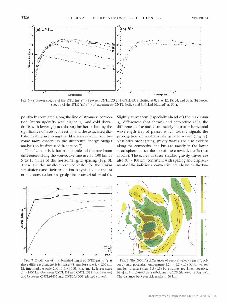
As in TZRS04, the spectral density of the initial ran-dom perturbation (white noise added only to the tem-perature field) is proportional to the magnitude of thehorizontal wavenumber vector (Fig. 6a). Despite a dra-matic decrease of DTE at the smallest scales (�100 km;Fig. 6a) over the first 3 h owing largely to model diffu-sion (see Snyder et al. 2003; TZRS04; Zhang et al.2006), the domain-integrated DTE increases signifi-cantly (Fig. 5), particularly at scales �150–200 km. Fig-ure 6a shows that the saturation of the error spectrumat scales smaller than 200 km is complete by 6 h andthat the error growth rate at intermediate scales (200km � L � 1000 km) decreases between 12 and 18 h.Consistent with the visual impression from the error

FIG. 3. The surface potential temperature (thin line, � � 6 K) and sea level pressure (thick line, � � 8 hPa) validat 9 h of the nested grid forecast simulated by experiments (a) CNTL-D3 (10-km run) and (b) CNTL-D4 (3.3-kmrun), both plotted on a subdomain of the 30-km grid. Also shown are the difference fields for (c) “CNTL-D3” �“CNTL-D2” and (d) “CNTL-D3” � “CNTL-D4” of the surface potential temperature (thin line, � � 2 K; dashed,negative) and sea level pressure (thick line, � � 2 hPa; dashed, negative) along with the sea level pressure fromCNTL-D3 (gray line, ��8 hPa). The rectangular box in (b) denotes the location of the 3.3-km nested domain D4.The distance between tick marks is 90 km.



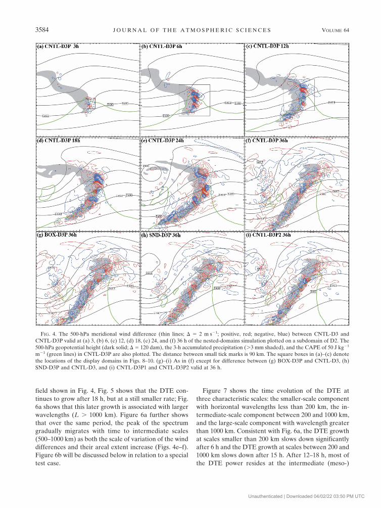
field shown in Fig. 4, Fig. 5 shows that the DTE con-tinues to grow after 18 h, but at a still smaller rate; Fig.6a shows that this later growth is associated with largerwavelengths (L � 1000 km). Figure 6a further showsthat over the same period, the peak of the spectrumgradually migrates with time to intermediate scales(500–1000 km) as both the scale of variation of the winddifferences and their areal extent increase (Figs. 4e–f).Figure 6b will be discussed below in relation to a specialtest case.

Figure 7 shows the time evolution of the DTE atthree characteristic scales: the smaller-scale componentwith horizontal wavelengths less than 200 km, the in-termediate-scale component between 200 and 1000 km,and the large-scale component with wavelength greaterthan 1000 km. Consistent with Fig. 6a, the DTE growthat scales smaller than 200 km slows down significantlyafter 6 h and the DTE growth at scales between 200 and1000 km slows down after 15 h. After 12–18 h, most ofthe DTE power resides at the intermediate (meso-)

FIG. 4. The 500-hPa meridional wind difference (thin lines; � � 2 m s�1; positive, red; negative, blue) between CNTL-D3 andCNTL-D3P valid at (a) 3, (b) 6, (c) 12, (d) 18, (e) 24, and (f) 36 h of the nested-domains simulation plotted on a subdomain of D2. The500-hPa geopotential height (dark solid; � � 120 dam), the 3-h accumulated precipitation (�3 mm shaded), and the CAPE of 50 J kg�1

m�1 (green lines) in CNTL-D3P are also plotted. The distance between small tick marks is 90 km. The square boxes in (a)–(c) denotethe locations of the display domains in Figs. 8–10. (g)–(i) As in (f) except for difference between (g) BOX-D3P and CNTL-D3, (h)SND-D3P and CNTL-D3, and (i) CNTL-D3P1 and CNTL-D3P2 valid at 36 h.


Fig 4 live 4/C


scales (200 km, 1000 km). Selection of the cutoff wave-lengths between the three scales is rather arbitrary butthe conclusions reached herein are not particularly sen-sitive to this choice.

The variation of difference growth with scale shownin Fig. 7 fits with the Lorenz (1969) picture of a systemwith a finite, intrinsic limit of predictability. Differencesgrow at the smallest (resolved) scale, where they satu-rate at relatively small amplitude. Differences at in-creasingly larger scales grow more and more slowly, butattain larger and larger amplitudes. The predictabilityof the largest scales is then limited by the rapid growthof differences at smaller scales.

In the present convection-permitting simulations, thedifferences grow and spread upscale in a manner that isqualitatively similar to that found in TZRS04 in its scaledependence (cf. Fig. 6a with Fig. 6 of TZRS04) butquantitatively much faster than those in the 30-kmsimulations of TZRS04 with parameterized convection(solid red curve with � symbols in Fig. 5). Much stron-ger error growth in the high-resolution convection-permitting experiments than the lower-resolution ex-periments was also found in Zhang et al. (2003) for the“surprise” snowstorm. This raises the question of howthe present results would be changed with further in-creases of resolution.

Figure 5 shows that changing the horizontal grid in-crements from 10 to 3.3 km leads to a larger errorgrowth rate in the first 3 h. Spectrum analysis of the3.3-km simulations (not shown) indicates that these

smaller-scale, faster-growing errors saturate after 3 hand hence the error at 9 h using the 3.3-km grid is onlyslightly smaller than it is on the 10-km grid. This be-havior is again consistent with a system having finiteintrinsic predictability. Moreover, going to higher reso-lution does not introduce qualitatively new dynamicsnor is the difference growth significantly more rapidafter the first 3 h. Hence for the remainder of this paperwe concentrate on the 10-km convection-permittingsimulations that appear to represent marginally well themesoscale aspects of moist convection and thus can beused to identify the error-growth dynamics for thesimulated moist baroclinic waves in this study.

5. A three-stage error-growth conceptual model

The convection-permitting experiments in the previ-ous section demonstrated that small-scale small-amplitude initial errors could grow rapidly and spreadupscale in the present simulations of moist baroclinicwaves. A closer examination of the difference betweenthe two 10-km simulations (CNTL-D3 and CNTL-D3P)discussed below suggests three distinct stages of errorgrowth.

a. Stage 1: Convective instability and saturation(0–6 h)

Figure 8 shows the differences of vertical velocity wand temperature T at 500 hPa between CNTL-D3 andCNTL-D3P valid at 3 h of the nested domain simula-tions in a 300-km square box indicated in Fig. 4a, wherethe maximum 500-hPa wind difference � occurs. Exami-nation of the differences of the total hydrometeor mix-ing ratio (qrc) (which includes cloud and precipitablewater/ice; not shown) reveals that this is also the area ofsignificant difference in moist processes. Differences inall fields grow in the area of strong moist convectionindicated by a high value of CAPE and heavy precipi-tation (Figs. 4a,b) collocated with significant qrc differ-ences. The 500-hPa T (w) difference grows from aninitial magnitude of 0.2 K (0 m s�1) to a maximum of�3 K (�7 m s�1) at 3 h (Fig. 8) and �7 K (�13 m s�1)at 6 h (not shown). The differences of w are also com-parable to the maximum values found in either CNTL-D3 or CNTL-D3P at these times (3–6 h), indicatingcomplete displacements of intense individual convec-tive cells between the unperturbed and perturbed simu-lations. Such displacements also imply local error satu-ration at the convective scales, consistent with the�-wind difference (Figs. 4a,b) and the evolution of DTEat scales below 200 km (Fig. 7) described above. More-over, maximum differences of qrc, w, and T are mostly

FIG. 5. Evolution of DTE (m2 s�2) integrated over a horizontalwavelength of the baroclinic wave estimated on the 30-km grid inexperiments with different model resolutions (i.e., CNTL 10 km,solid; 30 km, solid with “�”; 3.3 km, solid with “*”) and initialperturbations (i.e., BOX-D3P, dashed with “�”; SND-D3P,dashed with “*”; CNTL-D3P2, dotted–dashed) and between thetwo fake-dry simulations (dashed).



positively correlated along the line of strongest convec-tion (warm updrafts with higher qrc and cold down-drafts with lower qrc; not shown) further indicating thesignificance of moist convection and the associated dia-batic heating in forcing the differences (which will be-come more evident in the difference energy budgetanalysis to be discussed in section 7).

The characteristic horizontal scales of the maximumdifferences along the convective line are 50–100 km or5 to 10 times of the horizontal grid spacing (Fig. 8).These are the smallest resolved scales for the 10-kmsimulations and their excitation is typically a signal ofmoist convection in gridpoint numerical models.

Slightly away from (especially ahead of) the maximumqrc differences (not shown) and convective cells, thedifferences of w and T are nearly a quarter horizontalwavelength out of phase, which usually signals thepropagation of smaller-scale gravity waves (Fig. 8).Vertically propagating gravity waves are also evidentalong the convective line but are mostly in the lowerstratosphere above the top of the convective cells (notshown). The scales of these smaller gravity waves arealso 50 � 100 km, consistent with spacing and displace-ment of the individual convective cells between the two

FIG. 6. (a) Power spectra of the DTE (m2 s�2) between CNTL-D3 and CNTL-D3P plotted at 0, 3, 6, 12, 18, 24, and 36 h. (b) Powerspectra of the DTE (m2 s�2) of experiments CNTL (solid) and CNTLfd (dashed) at 36 h.

FIG. 7. Evolution of the domain-integrated DTE (m2 s�2) atthree different characteristics scales (S: smaller-scale L � 200 km;M: intermediate-scale 200 � L � 1000 km; and L: larger-scaleL � 1000 km), between CNTL-D3 and CNTL-D3P (solid curves)and between CNTLfd-D3 and CNTLfd-D3P (dotted curves).

FIG. 8. The 500-hPa differences of vertical velocity (m s�1, col-ored) and potential temperature [� � 0.2 (1.0) K for valuessmaller (greater) than 0.5 (1.0) K; positive, red lines; negative,blue] at 3 h plotted on a subdomain of D3 (denoted in Fig. 4a).The distance between tick marks is 30 km.


Fig 8 live 4/C


simulations. These smaller scale gravity waves may dis-perse the error energy from the area of active moistconvection.

Similar error-growth characteristics are also ob-served between CNTL-D4 and CNTL-D3 (Fig. 3d) aswell as between CNTL-D4 and CNTL-D4P (errorgrowth in the 3.3-km runs) interpolated to the 10-kmgrids at similar locations (not shown). The associationof the initial error growth with conditional instabilityand moist convection was also found in Zhang et al.(2002, 2003), and TZRS04 and showed that moist con-vection is responsible for the rapid initial error growthin the simulations.

b. Stage 2: Transition and adjustment (3–18 h)

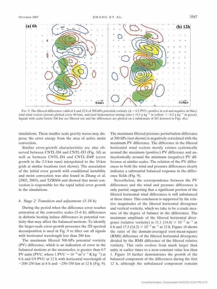
During the period when the difference error reachessaturation at the convective scales (3–6 h), differencesin diabatic heating induce differences in potential vor-ticity that may affect the balanced motions. To identifythe larger-scale error-growth processes the 2D spectraldecomposition is used in Fig. 9 to filter out all signalswith horizontal wavelength less than 200 km.

The maximum filtered 500-hPa potential vorticity(PV) difference, which is an indication of error in thebalanced motions at the mesoscales, is greater than 0.7PV units (PVU, where 1 PVU � 10�6 m2 s�1 K kg�1) at6 h and 0.9 PVU at 12 h with horizontal wavelength of�200–250 km at 6 h and �250–350 km at 12 h (Fig. 9).

The maximum filtered pressure perturbation differenceat 500 hPa (not shown) is negatively correlated with themaximum PV difference. The difference in the filteredhorizontal wind vectors mostly rotates cyclonicallyaround the maximum (positive) PV difference and an-ticyclonically around the minimum (negative) PV dif-ference at similar scales. The relation of the PV differ-ences to both the wind and pressure differences clearlyindicates a substantial balanced response in the differ-ence fields (Fig. 9).

Nevertheless, the correspondence between the PVdifferences and the wind and pressure differences isonly partial, suggesting that a significant portion of thefiltered horizontal wind differences is still unbalancedat these times. This conclusion is supported by the rela-tive magnitudes of the filtered horizontal divergenceand vertical vorticity, which we take to be a crude mea-sure of the degree of balance in the differences. Themaximum amplitude of the filtered horizontal diver-gence (relative vorticity) is 11.1 (14.4) � 10�5 m�1 at6 h and 17.3 (24.2) � 10�5 m�1 at 12 h. Figure 10 showsthe ratio of the domain-averaged root-mean-square(RMS) difference of the filtered horizontal divergencedivided by the RMS difference of the filtered relativevorticity. This ratio evolves from much larger thanunity at earlier times to a near-constant value less than1. Figure 10 further demonstrates the growth of thebalanced component of the differences during the first12 h, although the unbalanced component remains

FIG. 9. The filtered differences valid at 6 and 12 h of 500-hPa potential vorticity (� � 0.2 PVU; positive in red and negative in blue),total wind vectors (arrows plotted every 60 km), and total hydrometeor mixing ratio (�0.3 g kg�1 in yellow; ��0.2 g kg�1 in green).Signals with scales below 200 km are filtered out and the differences are plotted on a subdomain of D2 denoted in Figs. 4b,c.


Fig 9 live 4/C


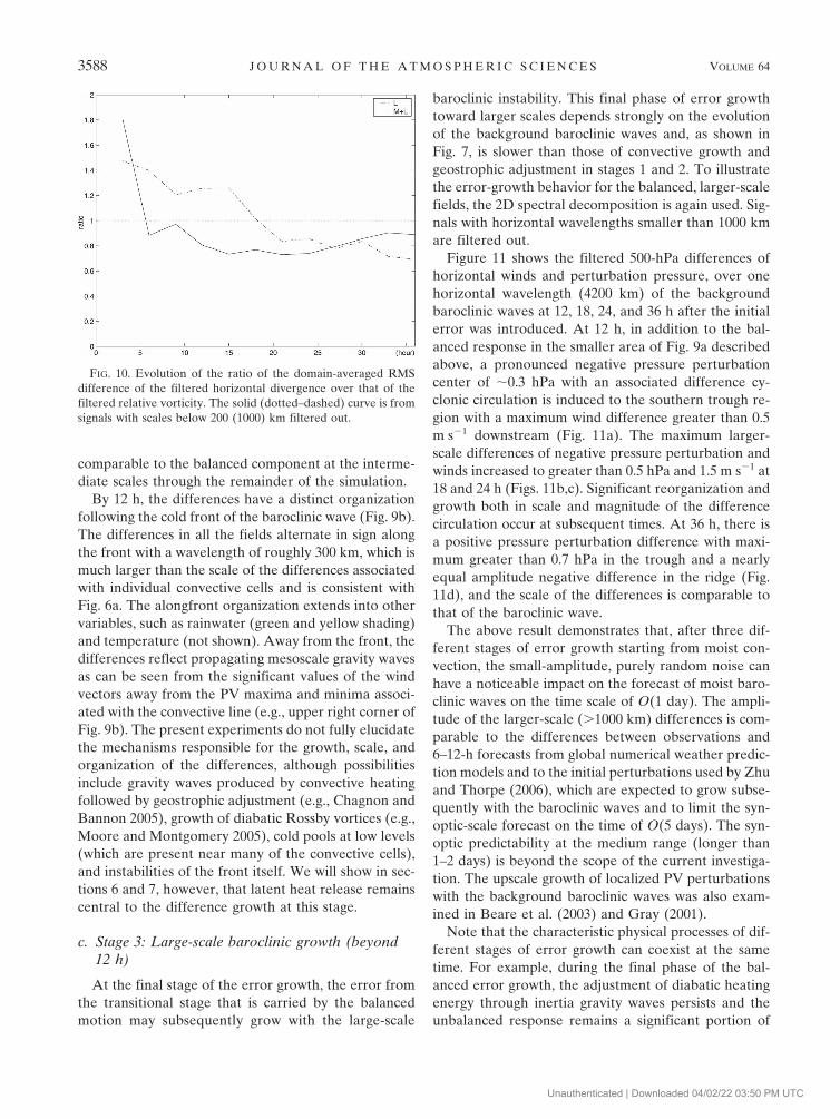
comparable to the balanced component at the interme-diate scales through the remainder of the simulation.

By 12 h, the differences have a distinct organizationfollowing the cold front of the baroclinic wave (Fig. 9b).The differences in all the fields alternate in sign alongthe front with a wavelength of roughly 300 km, which ismuch larger than the scale of the differences associatedwith individual convective cells and is consistent withFig. 6a. The alongfront organization extends into othervariables, such as rainwater (green and yellow shading)and temperature (not shown). Away from the front, thedifferences reflect propagating mesoscale gravity wavesas can be seen from the significant values of the windvectors away from the PV maxima and minima associ-ated with the convective line (e.g., upper right corner ofFig. 9b). The present experiments do not fully elucidatethe mechanisms responsible for the growth, scale, andorganization of the differences, although possibilitiesinclude gravity waves produced by convective heatingfollowed by geostrophic adjustment (e.g., Chagnon andBannon 2005), growth of diabatic Rossby vortices (e.g.,Moore and Montgomery 2005), cold pools at low levels(which are present near many of the convective cells),and instabilities of the front itself. We will show in sec-tions 6 and 7, however, that latent heat release remainscentral to the difference growth at this stage.

c. Stage 3: Large-scale baroclinic growth (beyond12 h)

At the final stage of the error growth, the error fromthe transitional stage that is carried by the balancedmotion may subsequently grow with the large-scale

baroclinic instability. This final phase of error growthtoward larger scales depends strongly on the evolutionof the background baroclinic waves and, as shown inFig. 7, is slower than those of convective growth andgeostrophic adjustment in stages 1 and 2. To illustratethe error-growth behavior for the balanced, larger-scalefields, the 2D spectral decomposition is again used. Sig-nals with horizontal wavelengths smaller than 1000 kmare filtered out.

Figure 11 shows the filtered 500-hPa differences ofhorizontal winds and perturbation pressure, over onehorizontal wavelength (4200 km) of the backgroundbaroclinic waves at 12, 18, 24, and 36 h after the initialerror was introduced. At 12 h, in addition to the bal-anced response in the smaller area of Fig. 9a describedabove, a pronounced negative pressure perturbationcenter of �0.3 hPa with an associated difference cy-clonic circulation is induced to the southern trough re-gion with a maximum wind difference greater than 0.5m s�1 downstream (Fig. 11a). The maximum larger-scale differences of negative pressure perturbation andwinds increased to greater than 0.5 hPa and 1.5 m s�1 at18 and 24 h (Figs. 11b,c). Significant reorganization andgrowth both in scale and magnitude of the differencecirculation occur at subsequent times. At 36 h, there isa positive pressure perturbation difference with maxi-mum greater than 0.7 hPa in the trough and a nearlyequal amplitude negative difference in the ridge (Fig.11d), and the scale of the differences is comparable tothat of the baroclinic wave.

The above result demonstrates that, after three dif-ferent stages of error growth starting from moist con-vection, the small-amplitude, purely random noise canhave a noticeable impact on the forecast of moist baro-clinic waves on the time scale of O(1 day). The ampli-tude of the larger-scale (�1000 km) differences is com-parable to the differences between observations and6–12-h forecasts from global numerical weather predic-tion models and to the initial perturbations used by Zhuand Thorpe (2006), which are expected to grow subse-quently with the baroclinic waves and to limit the syn-optic-scale forecast on the time of O(5 days). The syn-optic predictability at the medium range (longer than1–2 days) is beyond the scope of the current investiga-tion. The upscale growth of localized PV perturbationswith the background baroclinic waves was also exam-ined in Beare et al. (2003) and Gray (2001).

Note that the characteristic physical processes of dif-ferent stages of error growth can coexist at the sametime. For example, during the final phase of the bal-anced error growth, the adjustment of diabatic heatingenergy through inertia gravity waves persists and theunbalanced response remains a significant portion of

FIG. 10. Evolution of the ratio of the domain-averaged RMSdifference of the filtered horizontal divergence over that of thefiltered relative vorticity. The solid (dotted–dashed) curve is fromsignals with scales below 200 (1000) km filtered out.



the total difference (Fig. 10). The difference in the in-ertia–gravity wave response (stage 2) may also triggerrapid error growth due to convective instability in thefar field (stage 1).

6. Sensitivity to initial perturbations and moisturecontents

The previous sections showed that the initial randomperturbations between CNTL-D3 (unperturbed) andCNTL-D3P (perturbed) experiments decayed every-

where except for a small region in the southeast quad-rant of the upper-level trough and surface cyclonewhere there is strong CAPE and sufficient low-levellifting. The significance of the rapid initial error growthin this small region of convective/conditional instabilitybecomes even more obvious in experiment “BOX-D3P,” which uses exactly the same perturbations as inCNTL-D3P but the perturbations are only applied onlyto the small shaded rectangular box of high CAPE de-noted in Fig. 1.

The evolution of the difference between CNTL-D3

FIG. 11. The filtered differences of the 500-hPa perturbation pressure (thick lines; � � 0.2 hPa; negative, dashed) and total windvectors (arrows with values greater than 0.5 shaded every 0.5 m s�1) along with the 500-hPa geopotential height from CNTL-D3P (thinlines, � � 120 dam) valid at (a) 12, (b) 18, (c) 24, and (d) 36 h. All signals with scales below 1000 km are filtered off and the differencesare plotted on a subdomain of D2. The distance between small tick marks is 90 km.



and BOX-D3P undergoes virtually the same multistageerror growth as described above. For example, the 500-hPa v-wind difference at 36 h (Fig. 4g) is comparable inhorizontal extent, scale, and magnitude to that betweenCNTL-D3 and CNTL-D3P (Fig. 4f). In terms of do-main-integrated DTE (Fig. 5, dotted curve with “�”),despite a much smaller initial difference (less than 5%),the DTE error between BOX-D3P and CNTL-D3grows to an amplitude comparable to that betweenCNTL-D3P and CNTL-D3 over the first 3 h and be-comes even slightly larger at 21 h with the trend con-tinued to 36 h. Experiment BOX-D3P further demon-strates that the effective error growth (between CNTL-D3 and CNTL-D3P) over the first 3 h is much strongerthan estimated from the domain-integrated DTE alone.Rapid error growth due to moist convection occurs ini-tially over the region of strong convective/conditionalinstability. This is also true even if we only perturbedone vertical column of the model grid (i.e., verticalsounding) inside the unstable region as in experiment“SND-D3P.”

The difference between CNTL-D3 and SND-D3Ptriggers a displacement of a convective cell at the verybeginning (not shown). Despite a 3–6-h delay of errorsaturation at the convective scales (suggested fromDTE in Fig. 5), the 500-hPa �-wind difference (Fig. 4h)and the DTE at 36 h (Fig. 5) between CNTL-D3 andBOX-D3P are again comparable in horizontal extent,scale, and magnitude to that between CNTL-D3 andCNTL-D3P (Fig. 4f). Similar evolution of the differ-ence field is also found between two perturbed experi-ments, that is, CNTL-D3P and another perturbed ex-periment, CNTL-D3P2, which is the same as in CNTL-D3P but with a different realization of randomperturbations (Fig. 4i and dotted–dashed curve inFig. 5).

We also examined the effects of initial moisture dis-tribution on mesoscale predictability with convection-permitting simulations, in which the initial relative hu-midity of domain D1 is reduced to 70%, 40%, and 0%of that in CNTL, for both perturbed and unperturbedsets of simulations. The same perturbations used forCNTL-D3P are used in the perturbed simulations.From both the v-wind difference and the domain-integrated DTE, significantly and decreasingly smallererror growth is found in these experiments with de-creasingly less moisture contents (not shown). Thesmaller difference with less moisture content occurs atall scales at 36 h compared to those between CNTL-D3and CNTL-D3P at this time (not shown). Consistentwith TZRS04, since the simulations with larger relativehumidity exhibit greater conditional instability andstronger moist convection, the relation between initial

humidity and error growth also supports our assertionthat the moist convection controls the initial phase ofthe error growth.

The aforementioned experiments and those fromTZRS04 and Zhang et al. (2003) further demonstratethat moist convection is essential in organizing and am-plifying small-scale small-amplitude disturbances overthe first 3–6 h of the simulations. One may ask whetherconvection (or moist processes) is necessary to sustainthe error growth after the difference energy has alreadygrown and spread to larger scales. An additional pair ofexperiments (“CNTLfd-D3” and “CNTLfd-D3P”) isperformed in a manner similar to CNTL except that,after 18 h of the nested domain integration, latent heat-ing/cooling from moist processes is turned off in boththe perturbed and unperturbed runs. The subsequentDTE evolution from CNTLfd is plotted in dashed curveof Fig. 5, from which one can see that the DTE dropsquickly and reduces to about half of its moist counter-part after another 18 h of “fake dry” integration. Theresult from the “fake dry” experiment further demon-strates fundamental differences exist between dry andmoist simulations in terms of mesoscale predictability.

The result from the present 10-km fake-dry simula-tions, however, is in strong contrast to the 30-km ex-periments with parameterized convection of TZRS04,in which the DTE drops by an order of magnitude afterthe turning off of latent heating (Fig. 11 of TZRS04).At the beginning of the fake-dry runs (18 h), thepresent 10-km experiment has a significantly larger por-tion of error (difference) at the larger scales (�1000km; Fig. 5) than that in TZRS04 (their Fig. 6). Since thelarger-scale difference is less affected by dissipation, itcan retain much of its amplitude while evolving with thebackground baroclinic waves. The dotted curves in Fig.6b show that reduction of the DTE error in the fake-drysimulations comes from all scales but most dramaticallyat smaller scales. For example, the 500-hPa �-wind dif-ferences from the fake-dry simulations at 24 and 36 h(Fig. 12) has a much smaller, localized, smaller-scalemaxima than those of CNTL (Figs. 4e,f), but the dif-ferences of the filtered large scale (�1000 km) of the500-hPa pressure perturbation and winds in the fake-dry runs (Fig. 13) are comparable in magnitude to thoseof CNTL (Figs. 11c,d). Noticeably, the larger-scale (andmore balanced) differences between CNTLfd simula-tions are similar in structure to those of CNTL at 24 h(Fig. 11c versus Fig. 13a) but they evolved into a sig-nificantly different larger-scale pattern at 36 h (Fig. 11dversus Fig. 13b), indicating that the error growth atstage 3 may also be significantly modulated by moistdynamics.



7. Budget analysis of difference kinetic energy

To further quantify the impacts of moist convectionand other physical processes on mesoscale predictabil-ity, a budget analysis of the difference kinetic energy(DKE) between the perturbed and unperturbed experi-ments is performed. The breakdown of the domain-integrated DKE tendency into different source and sinkterms resembles closely the budget analysis of turbulentkinetic energy (TKE; Stull 1989; Holton 1992). Thesource and sink terms include buoyancy production orloss (which also includes hydrometer drag), nonlinearvelocity advection (or shear production), redistribution,and net production by pressure gradient force, and dis-

sipation due to horizontal and vertical diffusions. Thederivation of the DKE equation and the formulationand estimation of each term in the DKE budget arepresented in the appendix.

The time evolution of the DKE tendency and each ofthe source/sink terms per area unit (i.e., integrated ver-tically) estimated with hourly model outputs from the10-km grid of CNTL-D3 and CNTL-D3P is plotted inFig. 14. Consistent with the DTE evolution plot in Fig.5, maximum DKE tendency (growth rate) occurs dur-ing the convective phase of error growth (stage 1) andpeaks at 4–5 h. A sharp decrease of the DKE growthfrom 5 to 7 h afterward coincides with the timing ofconvective-scale error saturation. During the adjust-

FIG. 12. As in Figs. 4e,f except for CNTLfd without precipitation valid at (a) 24 and (b) 36 h.

FIG. 13. As in Figs. 10c,d except for CNTLfd valid at (a) 24 and (b) 36 h.



ment period (7–12 h), the growth rate holds rathersteady (stage 2). After a brief secondary maximum at13 h, the DKE growth rate again falls considerably af-terward. It becomes negative from 28 to 31 h but re-covers to slightly positive for the final period of thesimulation.

From the evolution of each term in the budget equa-tion, it is found that buoyancy and nonlinear velocityadvection are the two dominant source terms for errorgrowth. These two terms are comparable in magnitudethroughout the 36-h simulation. Further budget analy-sis of the thermodynamic equation (not shown) dem-onstrates that the buoyancy term comes primarily fromdiabatic heating due to moist convection. In otherwords, through warm updraft or cold downdraft (e.g.,Fig. 8), the buoyancy term (i.e., vertical heat flux) re-distributes diabatic heating from moist convection. Thepressure force term is also positive but is less than 20%of the buoyancy or advection term. Except for the firstfew hours, these source terms are nearly balanced withthe dissipation terms due to horizontal and vertical dif-fusion, which result in a small overall DKE growth (Fig.3a).

The DKE budgets analysis is also performed for ex-periment CNTLfd (dotted curves in Fig. 14). As ex-pected, the cessation of diabatic heating immediatelyleads to a dramatic decrease of buoyancy contribution(to less than 10% of its original magnitude). Moreover,the switching off of diabatic heating also leads to asharp, immediate decrease in the nonlinear velocity ad-vection (to less than 20% of its original magnitude). Arelatively slower response (decrease) in the dissipation

terms leads to a large negative DKE tendency over thefirst few hours of the fake-dry simulations. The overallDKE tendency then equilibrates to nearly zero at 30 h.Budget analysis of the fake-dry experiment suggeststhat moist convection is not only crucial to the errorgrowth in terms of buoyancy production, but it alsoleads to large shear production. In other words, numer-ous small but vigorous eddies due to moist convectioncan efficiently transport both heat and momentum andthus contribute to larger magnitude of both buoyancyproduction and nonlinear velocity advection in theDKE budget. It is worth noting that only nonlinearvelocity advection is included in the error growth modelof the pioneering predictability study of Lorenz (1969).

8. Summary and discussion

A recent study by the authors examined the predict-ability of an idealized baroclinic wave amplifying in aconditionally unstable atmosphere through numericalsimulations with parameterized moist convection. Itwas demonstrated that with the effect of moisture in-cluded, the error starting from small random noise ischaracterized by upscale growth in the short term (0–36h) forecast of a rapidly growing synoptic-scale distur-bance. The current study seeks to further explore themesoscale error-growth dynamics in the idealized moistbaroclinic waves through convection-permitting experi-ments with model grid increments down to 3.3 km.

A multistage error-growth conceptual model is pro-posed. In the initial stage, the errors first grow fromsmall-scale convective instability and then quickly satu-rate at the convective scales on time scales of O(1 h).The amplitude of saturation errors may be a function ofCAPE and its areal coverage determined by large-scaleflows. In the transitional stage, the errors transformfrom convective-scale unbalanced motions to larger-scale balanced motions likely through geostrophic ad-justment on the time scale of O(1/f ). Part of the errorsdue to difference in latent heating from convection maybe retained in the balance fields while the others areradiating away in the form of gravity waves. In the finalstage, the balanced components of the errors in thelarger-scale flow grow with the background baroclinicinstability. Though an examination of the difference-error energy budget, similar to the turbulence kineticenergy budget analysis, it is found that buoyancy pro-duction due mostly to moist convection is comparableto shear production due to nonlinear advection. Notonly does turning off latent heating dramatically de-crease buoyancy production, but it also reduces shearproduction (nonlinear velocity advection) to less than20% of its original amplitude. These new findings fur-

FIG. 14. Time evolution of the DKE tendency and each of thesource/sink terms (J m�2 s�1) estimated with the 10-km gridhourly outputs from CNTL-D3 and CNTL-D3P (solid) and fromCNTLfd-D3 and CNTLfd-D3P (dashed).



ther demonstrate the effects of moist convection anddiabatic heating on the limit of mesoscale predictabil-ity.

Acknowledgments. The authors benefited fromdiscussions with Zhe-Min Tan, Steve Tracton, MikeMontgomery, Lance Bosart, and Craig Bishop. This re-search is funded by the U.S. Office of Naval Researchthrough the Young Investigator’s Program (AwardN000140410471).

APPENDIX

The Difference Kinetic Energy Budget Equation

In an f plane without topography as used in our ide-alized simulations, the MM5 model is essentially usinga height vertical coordinate and the momentum equa-tions can be simplified as

�u

�t� �v · �u �

1�

�p�

�x� f� � Du, A1�

��

�t� �v · ��

1�

�p�

�y� fu � D�, A2�

�w

�t� �v · �w �

1�

�p�

�z�

�

�0g � gqc � qr� � Dw,

A3�

where the last term of each equation represents thevertical and horizontal diffusion including vertical mix-ing due to the planetary boundary layer turbulence and/or dry convective adjustment.

To investigate the evolution of difference kinetic en-ergy between perturbed and unperturbed simulations,we subtract the above momentum equations from thecorresponding momentum equation for the perturbedsimulation that has the same form as the above equa-tions, resulting in

��u

�t� ��v · �u� � ��1

�

�p�

�x � � f�� Du, A4�

��

�t� ��v · �� 1

�

�p�

�y � � f�u � �D�, A5�

��w

�t� ��v · �w� � ��1

�

�p�

�z ��g

�0�� g�qc � �qr�

� �Dw. A6�

We further multiply Eqs. (A4)–(A6) by their respectivemomentum differences (i.e., �0�u, �0��, and �0�w) andthe sum of the resulting equations can be expressedsymbolically as follows:

�

�tDKE� � ��0�u�v · �u� � ��v · �� w�v · �w�

velocity advection�shear production term

� �0��u��1�

�p�

�x � � ��1�

�p�

�y � � �w��1�

�p�

�z ��pressure gradient forcing term

� �0� g

�0�w�� g�qc � �qr�w�

buoyancy term including hydrometer drag�

� �0�u�Du � �v�D�

horizontal diffusion

� �0�w�Dw

vertical diffusion

, A7�

where the DKE is defined as

DKE ��0

2�u�2 � ��2 � �w�2 . A8�

REFERENCES

Anthes, R. A., Y. H. Kuo, D. P. Baumhefner, R. P. Errico, andT. W. Bettge, 1985: Predictability of mesoscale atmosphericmotions. Advances in Geophysics, Vol. 28B, Academic Press,159–202.

Beare, R. J., A. J. Thorpe, and A. A. White, 2003: The predict-ability of extratropical cyclones: Nonlinear sensitivity to po-tential vorticity perturbations. Quart. J. Roy. Meteor. Soc.,129, 219–237.

Boffetta, G., A. Celani, A. Crisanti, and A. Vulpiani, 1996: Pre-dictability in two-dimensional decaying turbulence. Phys.Fluids, 9, 724–734.

Bryan, G. H., J. C. Wyngaard, and J. M. Fritsch, 2003: Resolution

requirements for the simulation of deep moist convection.Mon. Wea. Rev., 131, 2394–2416.

Chagnon, J. M., and P. R. Bannon, 2005: Wave response duringhydrostatic and geostrophic adjustment. Part I: Transient dy-namics. J. Atmos. Sci., 62, 1311–1329.

Dudhia, J., 1993: A nonhydrostatic version of the Penn State–NCAR Mesoscale Model: Validation tests and simulation ofan Atlantic cyclone and cold front. Mon. Wea. Rev., 121,1493–1513.

Errico, R., and D. Baumhefner, 1987: Predictability experimentsusing a high-resolution limited-area model. Mon. Wea. Rev.,115, 488–504.

Gray, M. E. B., 2001: The impact of mesoscale convective-systempotential-vorticity anomalies on numerical-weather-prediction forecasts. Quart. J. Roy. Meteor. Soc., 127, 73–88.

Grell, G. A., 1993: Prognostic evaluation of assumptions used bycumulus parameterizations. Mon. Wea. Rev., 121, 764–787.

Holton, J. R., 1992: An Introduction to Dynamic Meteorology.Academic Press, 511 pp.



Hong, S.-Y., and H.-L. Pan, 1996: Nonlocal boundary layer ver-tical diffusion in a medium-range forecast model. Mon. Wea.Rev., 124, 2322–2339.

Leith, C. E., 1971: Atmospheric predictability and two-dimen-sional turbulence. J. Atmos. Sci., 28, 145–161.

——, and R. H. Kraichnan, 1972: Predictability of turbulent flows.J. Atmos. Sci., 29, 1041–1058.

Lilly, D. K., 1972: Numerical simulation studies of two-dimensional turbulence. II. Stability and predictability stud-ies. Geophys. Astrophys. Fluid Dyn., 4, 1–28.

Lorenz, E. N., 1969: The predictability of a flow which possessesmany scales of motion. Tellus, 21, 289–307.

Metais, O., and M. Lesieur, 1986: Statistical predictability of de-caying turbulence. J. Atmos. Sci., 43, 857–870.

Moore, R. W., and M. T. Montgomery, 2005: Analysis of an ide-alized, three-dimensional diabatic rossby vortex: A coherentstructure of the moist baroclinic atmosphere. J. Atmos. Sci.,62, 2703–2725.

Nuss, W. A., and D. K. Miller, 2001: Mesoscale predictability un-der various synoptic regimes. Nonlinear Processes Geophys.,8, 429–438.

Pielke, R. A., G. A. Dalu, J. S. Snook, T. J. Lee, and T. G. F.Kittel, 1991: Nonlinear influence of mesoscale land use onweather and climate. J. Climate, 4, 1053–1069.

Rotunno, R., and J.-W. Bao, 1996: A case study of cyclogenesisusing a model hierarch. Mon. Wea. Rev., 124, 1051–1066.

Shapiro, M. A., and Coauthors, 1999: A planetary-scale to meso-

scale perspective of the life cycles of extratropical cyclones.The Life Cycles of Extratropical Cyclones, M. A. Shapiro andS. Gronas., Eds., Amer. Meteor. Soc., 1228–1251.

Snyder, C., T. M. Hamill, and S. B. Trier, 2003: Linear evolutionof error covariances in a quasigeostrophic model. Mon. Wea.Rev., 131, 189–205.

Stull, R. B., 1989: An Introduction to Boundary Layer Meteorol-ogy. Kluwer, 680 pp.

Tan, Z.-M., F. Zhang, R. Rotunno, and C. Snyder, 2004: Meso-scale predictability of moist baroclinic waves: Experimentswith parameterized convection. J. Atmos. Sci., 61, 1794–1804.

Vukicevic, T., and R. M. Errico, 1990: The influence of artificialand physical factors upon predictability estimates using acomplex limited-area model. Mon. Wea. Rev., 118, 1460–1482.

Zhang, F., C. Snyder, and R. Rotunno, 2002: Mesoscale predict-ability of the “surprise” snowstorm of 24–25 January 2000.Mon. Wea. Rev., 130, 1617–1632.

——, ——, and ——, 2003: Effects of moist convection on meso-scale predictability. J. Atmos. Sci., 60, 1173–1185.

——, A. Odins, and J. W. Nielsen-Gammon, 2006: Mesoscale pre-dictability of an extreme warm-season rainfall event. Wea.Forecasting, 21, 149–166.

Zhu, H., and A. Thorpe, 2006: Predictability of extratropical cy-clones: The influence of initial condition and model uncer-tainties. J. Atmos. Sci., 63, 1483–1497.



mesoscale predictability of moist baroclinic waves

Documents