scaling baroclinic eddy fluxes: vortices and energy balance · scaling baroclinic eddy fluxes:...

Scaling Baroclinic Eddy Fluxes: Vortices and Energy Balance

ANDREW F. THOMPSON AND WILLIAM R. YOUNG

Scripps Institution of Oceanography, University of California, San Diego, La Jolla, California

(Manuscript received 26 April 2005, in final form 19 September 2005)

ABSTRACT

The eddy heat flux generated by the statistically equilibrated baroclinic instability of a uniform, horizontaltemperature gradient is studied using a two-mode f-plane quasigeostrophic model. An overview of thedependence of the eddy diffusivity D on the bottom friction �, the deformation radius �, the verticalvariation of the large-scale flow U, and the domain size L is provided by numerical simulations at 70different values of the two nondimensional control parameters ��/U and L/�. Strong, axisymmetric, well-separated baroclinic vortices dominate both the barotropic vorticity and the temperature fields. The coreradius of a single vortex is significantly larger than � but smaller than the eddy mixing length �mix. On theother hand, the typical vortex separation is comparable to �mix. Anticyclonic vortices are hot, and cyclonicvortices are cold. The motion of a single vortex is due to barotropic advection by other distant vortices, andthe eddy heat flux is due to the systematic migration of hot anticyclones northward and cold cyclonessouthward. These features can be explained by scaling arguments and an analysis of the statistically steadyenergy balance. These arguments result in a relation between D and �mix. Earlier scaling theories based oncoupled Kolmogorovian cascades do not account for these coherent structures and are shown to be unre-liable. All of the major properties of this dilute vortex gas are exponentially sensitive to the strength of thebottom drag. As the bottom drag decreases, both the vortex cores and the vortex separation become larger.Provided that �mix remains significantly smaller than the domain size, then local mixing length argumentsare applicable, and our main empirical result is �mix � 4� exp(0.3U/��).

1. Introduction

Eddy heat and potential vorticity fluxes are part of adynamical balance in which potential energy created bydifferential heating is released through baroclinic insta-bility. Many theoretical and numerical studies have at-tempted to find physically plausible parameterizationsof these eddy fluxes so that turbulent transport can beincluded in coarsely resolved climate models. Pioneer-ing attempts used linear theory to describe the eddystructure and energy arguments to constrain the eddyamplitude (Green 1970; Stone 1972). More recently,though, fully nonlinear numerical realizations of homo-geneous quasigeostrophic turbulence have been used todiagnose eddy fluxes in a statistical steady state main-tained by imposing a uniform temperature gradient(Haidvogel and Held 1980; Hua and Haidvogel 1986;

Larichev and Held 1995; Held and Larichev 1996;Smith and Vallis 2002; Lapeyre and Held 2003). Thegrail is a physically motivated relation between theeddy flux of heat and control parameters, such as theimposed large-scale thermal gradient. Provided thatthere is scale separation between the mean and theeddies, the resulting flux–gradient relation might applyapproximately to a spatially inhomogeneous flow. Inother words, the hypothesis is that baroclinic eddyfluxes can be parameterized by a turbulent diffusivityD, which might, however, depend nonlinearly on thelarge-scale temperature gradient (e.g., Pavan and Held1996). Our first goal in this work is largely descriptive:we characterize the dependence of D on external pa-rameters such as the domain size L, the bottom dragcoefficient �, the Rossby deformation radius �, and theimposed velocity jump U. Our notation is introducedsystematically in appendix A and is largely the same asthat of Larichev and Held (1995, hereinafter LH95):�(x, y, t) and �(x, y, t) are the disturbance streamfunc-tions of the baroclinic and barotropic modes, respec-tively. A precise definition of the eddy diffusivity D is

Corresponding author address: Andrew Thompson, Scripps In-stitution of Oceanography, University of California, San Diego,La Jolla, CA 92093-0213.E-mail: [email protected]

720 J O U R N A L O F P H Y S I C A L O C E A N O G R A P H Y VOLUME 36

© 2006 American Meteorological Society

JPO2874

then

D � U�1��x�. 1�

Here � denotes both a horizontal average over thesquare 2�L 2�L domain and an additional time av-erage to remove residual turbulent pulsations.

In (1), ��x� is the product of the barotropic meridi-onal velocity �x and the thermal field � ; that is, themeridional heat flux is proportional to ��x�. Moreover,the mechanical energy balance in a statistically steadystate (see appendix A) is

U��2��x� � ��|�� 2��|2 � hyp�, 2�

where “hyp�” indicates the hyperviscous dissipation ofenergy. The first term on the right-hand side of (2) isthe mechanical energy dissipation (watts per kilogram)by bottom drag, �. The left-hand side of (2) is the en-ergy extracted from the unstable horizontal tempera-ture gradient by baroclinic instability. Enstrophy bud-gets also identify ��x� as the large-scale source balanc-ing the hyperviscous enstrophy sink at highwavenumbers. Thus, a single quantity, conveniently de-fined as D in (1), summarizes all of the important qua-dratic power integrals and fluxes in homogeneous baro-clinic turbulence.

Dimensional considerations (Haidvogel and Held1980) show that

D � U� D*��

L,��

U,

�

UL7�, 3�

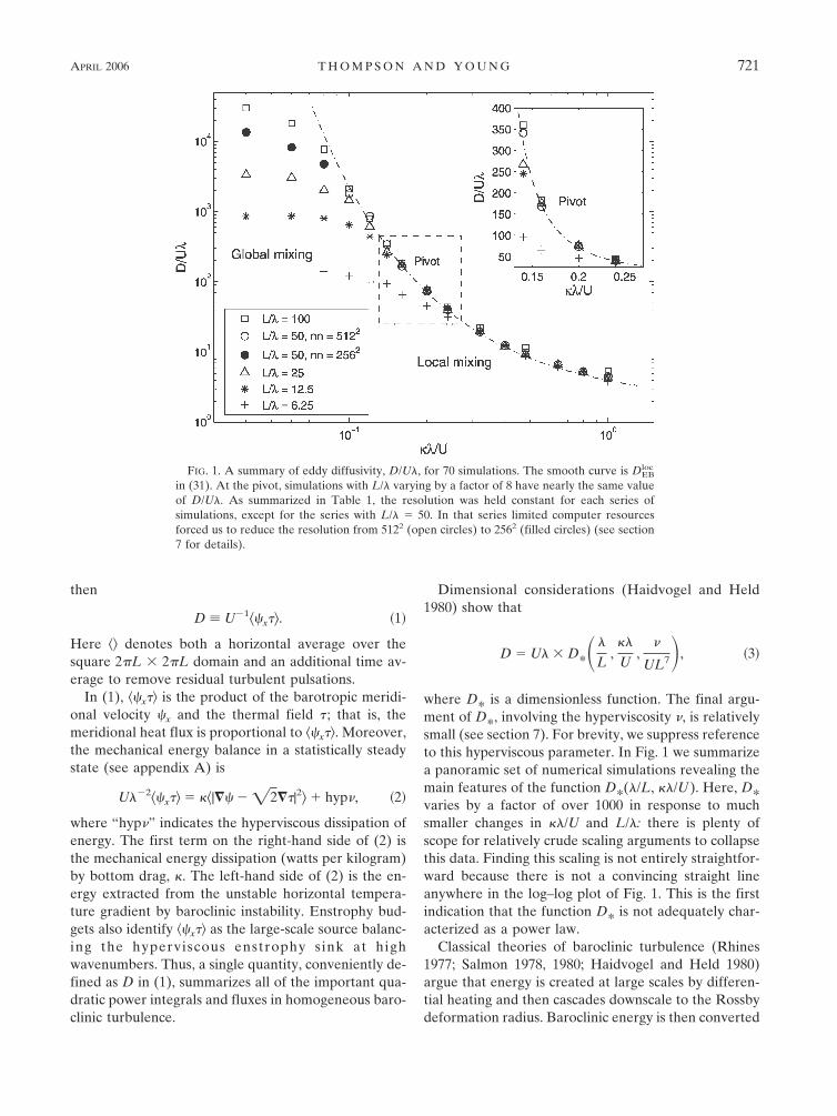
where D* is a dimensionless function. The final argu-ment of D*, involving the hyperviscosity �, is relativelysmall (see section 7). For brevity, we suppress referenceto this hyperviscous parameter. In Fig. 1 we summarizea panoramic set of numerical simulations revealing themain features of the function D*(�/L, ��/U). Here, D*varies by a factor of over 1000 in response to muchsmaller changes in ��/U and L/�: there is plenty ofscope for relatively crude scaling arguments to collapsethis data. Finding this scaling is not entirely straightfor-ward because there is not a convincing straight lineanywhere in the log–log plot of Fig. 1. This is the firstindication that the function D* is not adequately char-acterized as a power law.

Classical theories of baroclinic turbulence (Rhines1977; Salmon 1978, 1980; Haidvogel and Held 1980)argue that energy is created at large scales by differen-tial heating and then cascades downscale to the Rossbydeformation radius. Baroclinic energy is then converted

FIG. 1. A summary of eddy diffusivity, D/U�, for 70 simulations. The smooth curve is DEBloc

in (31). At the pivot, simulations with L/� varying by a factor of 8 have nearly the same valueof D/U�. As summarized in Table 1, the resolution was held constant for each series ofsimulations, except for the series with L/� � 50. In that series limited computer resourcesforced us to reduce the resolution from 5122 (open circles) to 2562 (filled circles) (see section7 for details).

APRIL 2006 T H O M P S O N A N D Y O U N G 721

to barotropic near the deformation radius, and thebarotropic mode undergoes an inverse cascade until en-ergy is removed by bottom drag. The dual-cascade sce-nario, summarized in Fig. 2, supposes that L � � so thatthere is spectral room for the cascades to operate. Thisregime, with the domain scale greatly exceeding theRossby deformation radius, is also oceanographicallyrelevant.

Early studies of baroclinic turbulence assumed thatthe mixing length of baroclinic eddies was comparableto �. In these circumstances, Haidvogel and Held (1980,hereinafter HH80) argued that eddy statistics should beindependent of the domain scale L. Varying the param-eter L/� between 7 and 15, HH80 provided evidence insupport of this hypothesis. The data in Fig. 1 span asignificantly larger range of L/� than does HH80 andfurther support their conclusion that D is independentof L provided that ��/U is not too small.

The proviso is necessary because Fig. 1 clearly showsan important distinction between two regimes: localmixing and global mixing. The local regime is exempli-fied by the point marked “pivot” in Fig. 1 (where ��/U� 0.16). At the pivot, four simulations with L/� varyingby a factor 8 have nearly the same D. The four pivotsolutions exemplify the “local mixing regime” of HH80,within which D is independent of L. However, as ��/Uis reduced to very small values, eddy length scales grow.Once the eddy mixing length is comparable to the do-main scale L, the system leaves the local mixing regime

and enters the global mixing regime, also indicated inFig. 1.

The notion of a diffusive parameterization, appli-cable to a slowly varying mean flow (Pavan and Held1996), is valid only in the local mixing regime. Thus, ourmain focus in the remainder of this paper is the char-acterization of the local regime.

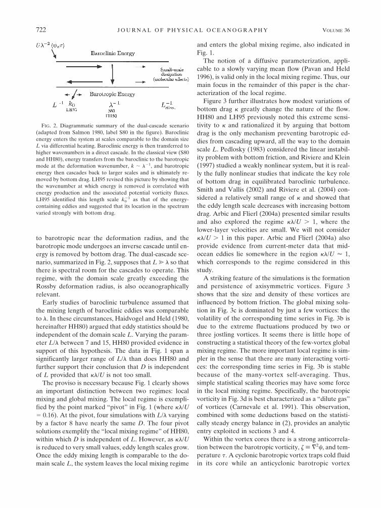
Figure 3 further illustrates how modest variations ofbottom drag � greatly change the nature of the flow.HH80 and LH95 previously noted this extreme sensi-tivity to � and rationalized it by arguing that bottomdrag is the only mechanism preventing barotropic ed-dies from cascading upward, all the way to the domainscale L. Pedlosky (1983) considered the linear instabil-ity problem with bottom friction, and Riviere and Klein(1997) studied a weakly nonlinear system, but it is real-ly the fully nonlinear studies that indicate the key roleof bottom drag in equilibrated baroclinic turbulence.Smith and Vallis (2002) and Riviere et al. (2004) con-sidered a relatively small range of � and showed thatthe eddy length scale decreases with increasing bottomdrag. Arbic and Flierl (2004a) presented similar resultsand also explored the regime ��/U � 1, where thelower-layer velocities are small. We will not consider��/U � 1 in this paper. Arbic and Flierl (2004a) alsoprovide evidence from current-meter data that mid-ocean eddies lie somewhere in the region ��/U � 1,which corresponds to the regime considered in thisstudy.

A striking feature of the simulations is the formationand persistence of axisymmetric vortices. Figure 3shows that the size and density of these vortices areinfluenced by bottom friction. The global mixing solu-tion in Fig. 3c is dominated by just a few vortices: thevolatility of the corresponding time series in Fig. 3b isdue to the extreme fluctuations produced by two orthree jostling vortices. It seems there is little hope ofconstructing a statistical theory of the few-vortex globalmixing regime. The more important local regime is sim-pler in the sense that there are many interacting vorti-ces: the corresponding time series in Fig. 3b is stablebecause of the many-vortex self-averaging. Thus,simple statistical scaling theories may have some forcein the local mixing regime. Specifically, the barotropicvorticity in Fig. 3d is best characterized as a “dilute gas”of vortices (Carnevale et al. 1991). This observation,combined with some deductions based on the statisti-cally steady energy balance in (2), provides an analyticentry exploited in sections 3 and 4.

Within the vortex cores there is a strong anticorrela-tion between the barotropic vorticity, � � �2�, and tem-perature � . A cyclonic barotropic vortex traps cold fluidin its core while an anticyclonic barotropic vortex

FIG. 2. Diagrammatic summary of the dual-cascade scenario(adapted from Salmon 1980, label S80 in the figure). Baroclinicenergy enters the system at scales comparable to the domain sizeL via differential heating. Baroclinic energy is then transferred tohigher wavenumbers in a direct cascade. In the classical view (S80and HH80), energy transfers from the baroclinic to the barotropicmode at the deformation wavenumber, k � ��1, and barotropicenergy then cascades back to larger scales and is ultimately re-moved by bottom drag. LH95 revised this picture by showing thatthe wavenumber at which energy is removed is correlated withenergy production and the associated potential vorticity fluxes.LH95 identified this length scale k0

�1 as that of the energy-containing eddies and suggested that its location in the spectrumvaried strongly with bottom drag.


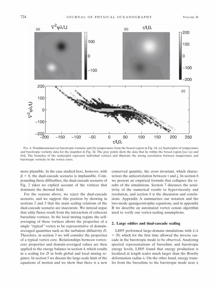
traps warm fluid in its core. Figures 4a and 4b showexpanded views of the barotropic vorticity and tem-perature, respectively, corresponding to the boxed re-gion in Fig. 3d. Figure 4c shows a scatterplot of tem-perature and barotropic vorticity from each point inFig. 3d. The scatterplot has a number of branches cor-responding to individual vortices such as those in Figs.4a and 4b (indicated by the gray points); therefore,most of the temperature anomaly is in the vortices. Themutual advection of these vortices is the main mecha-nism by which heat is transported meridionally in thissystem.

LH95 showed that the potential vorticity flux and themeridional heat flux (both of which are proportional toD) are dominated by the largest length scales excited bythe inverse cascade. LH95 associated the length k0

�1 �

� with both the mixing length and the peak of the baro-tropic energy spectrum. LH95 then used the dual-cascade model as a framework to derive a scaling forthe diffusive parameterization of the eddy fluxes (formore detail see section 2).

However, if the bottom drag is strong enough to limitthe inverse cascade to scales less than L, then argu-ments based on inertial energy-conserving spectralfluxes are invalid. In addition, if bottom drag is suffi-ciently small to allow a relatively undamped inversecascade, then barotropic energy accumulates at the do-main size, which is just the global mixing regime in Fig.1. In Held and Larichev (1996) and Lapeyre and Held(2003), this concern is ameliorated because a planetarypotential vorticity gradient � halts the inverse cascadewithout damping, so that the dual-cascade scenario is

FIG. 3. (a) Growth rates of the linear baroclinic instability problem for different values of the bottom drag parameter. (b) Time seriesof eddy diffusivity for different values of ��/U. The “instantaneous diffusivity” shown in these time series is defined by taking � in (1)only as an (x, y) average. (c), (d) Snapshots of the vorticity of the barotropic mode, �2��/U. In (b)–(d), L/� � 25. The box appearingin (d) is expanded in Fig. 4.


more plausible. In the case studied here, however, with� � 0, the dual-cascade scenario is implausible. Com-pounding these difficulties, the dual-cascade scenario ofFig. 2 takes no explicit account of the vortices thatdominate the thermal field.

For the reasons above, we reject the dual-cascadescenario, and we support this position by showing insections 2 and 3 that the main scaling relations of thedual-cascade scenario are inaccurate. We instead arguethat eddy fluxes result from the interaction of coherentbaroclinic vortices. In the local mixing regime the self-averaging of these vortices allows the properties of asingle “typical” vortex to be representative of domain-averaged quantities such as the turbulent diffusivity D.Therefore, in section 3 we will consider the propertiesof a typical vortex core. Relationships between vortex-core properties and domain-averaged values are thenapplied to the energy balance in section 4, which resultsin a scaling for D in both global and local mixing re-gimes. In section 5 we discuss the large-scale limit of theequations of motion and we show that there is a new

conserved quantity, the cross invariant, which charac-terizes the anticorrelation between � and �. In section 6we present an empirical formula that collapses the re-sults of the simulations. Section 7 discusses the sensi-tivity of the numerical results to hyperviscosity andresolution, and section 8 is the discussion and conclu-sions. Appendix A summarizes our notation and thetwo-mode quasigeostrophic equations, and in appendixB we describe an automated vortex census algorithmused to verify our vortex-scaling assumptions.

2. Large eddies and dual-cascade scaling

LH95 performed large-domain simulations with L/�� 50, which for the first time allowed the inverse cas-cade in the barotropic mode to be observed. Analyzingspectral representations of baroclinic and barotropicenergy levels, LH95 found that energy production islocalized at length scales much larger than the Rossbydeformation radius �. On the other hand, energy trans-fer from the baroclinic to the barotropic mode near �

FIG. 4. Nondimensional (a) barotropic vorticity and (b) temperature from the boxed region in Fig. 3d. (c) Scatterplot of temperatureand barotropic vorticity data for the snapshot in Fig. 3d. The gray points show the data that lie within the boxed region [see (a) and(b)]. The branches of the scatterplot represent individual vortices and illustrate the strong correlation between temperature andbarotropic vorticity in the vortex cores.


plays the passive, but important, role of energizing theinverse cascade. LH95 then proposed a revision to thetheory of HH80 and Salmon (1980) by arguing that theappropriate mixing length should be k0

�1, not �. LH95identified k0 as the wavenumber corresponding to thepeak in the barotropic energy spectrum; that is, k0 isboth the wavenumber of the energy-containing eddiesand the inverse of the mixing length. This modificationof the dual-cascade scenario is indicated in Fig. 2 by thearrow labeled LH95. Figure 2 also indicates that theexact location of k0 along the barotropic spectrum canvary dramatically due to a strong dependence on bot-tom friction.

LH95 then proceeded to estimate the eddy dif-fusivity as

D � characteristic barotropic velocity V

mixing length. 4�

Retaining the dual-cascade scenario as an interpreta-tive framework, and taking k0

�1 as the mixing length,LH95 argue that V � U/k0�. Thus, once the dust settles,the final result is the dual-cascade scaling

DDC � U�k02�. 5�

The strong dependence of DDC on bottom drag � is im-

plicit in k0, but no relationship between k0 and � wasproposed by LH95.

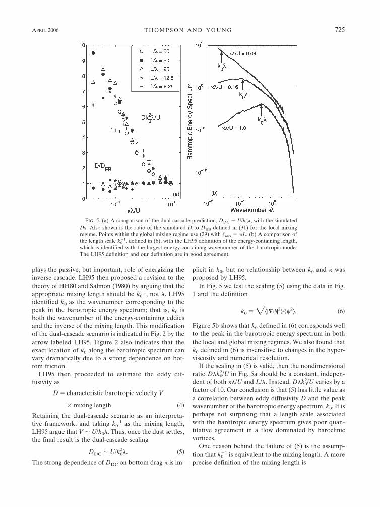
In Fig. 5 we test the scaling (5) using the data in Fig.1 and the definition

k0 � ��|��|2��2. 6�

Figure 5b shows that k0 defined in (6) corresponds wellto the peak in the barotropic energy spectrum in boththe local and global mixing regimes. We also found thatk0 defined in (6) is insensitive to changes in the hyper-viscosity and numerical resolution.

If the scaling in (5) is valid, then the nondimensionalratio D�k0

2/U in Fig. 5a should be a constant, indepen-dent of both ��/U and L/�. Instead, D�k0

2/U varies by afactor of 10. Our conclusion is that (5) has little value asa correlation between eddy diffusivity D and the peakwavenumber of the barotropic energy spectrum, k0. It isperhaps not surprising that a length scale associatedwith the barotropic energy spectrum gives poor quan-titative agreement in a flow dominated by baroclinicvortices.

One reason behind the failure of (5) is the assump-tion that k0

�1 is equivalent to the mixing length. A moreprecise definition of the mixing length is

FIG. 5. (a) A comparison of the dual-cascade prediction, DDC � U/k02�, with the simulated

Ds. Also shown is the ratio of the simulated D to DEB defined in (31) for the local mixingregime. Points within the global mixing regime use (29) with �mix � �L. (b) A comparison ofthe length scale k0

�1, defined in (6), with the LH95 definition of the energy-containing length,which is identified with the largest energy-containing wavenumber of the barotropic mode.The LH95 definition and our definition are in good agreement.


�mix � U�1��2. 7�

According to this definition, �mix times the basic-state �gradient, U, is equal to the root-mean-square fluctua-tion, ��2. This definition of the mixing length is con-sistent with the large-scale limit of the governing equa-tions in which the baroclinic evolution equation reducesto the advection of the quasi-passive scalar � by thebarotropic flow (see section 5).

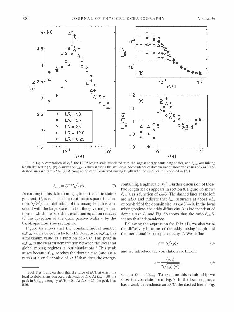
Figure 6a shows that the nondimensional numberk0�mix varies by over a factor of 2. Moreover, k0�mix hasa maximum value as a function of ��/U. This peak ink0�mix is the clearest demarcation between the local andglobal mixing regimes in our simulations.1 This peakarises because �mix reaches the domain size (and satu-rates) at a smaller value of ��/U than does the energy-

containing length scale, k0�1. Further discussion of these

two length scales appears in section 8. Figure 6b shows�mix/� as a function of ��/U. The dashed lines at the leftare �L/� and indicate that �mix saturates at about �L,or one-half of the domain size, as ��/U → 0. In the localmixing regime, the eddy diffusivity D is independent ofdomain size L, and Fig. 6b shows that the ratio �mix/�shares this independence.

Following the expression for D in (4), we also writethe diffusivity in terms of the eddy mixing length andthe meridional barotropic velocity V. We define

V � ��x2, 8�

and we introduce the correlation coefficient

c ��x�

��x2��2

, 9�

so that D � cV�mix. To examine this relationship weshow the correlation c in Fig. 7. In the local regime, chas a weak dependence on ��/U: the dashed line in Fig.

1 Both Figs. 1 and 6a show that the value of ��/U at which thelocal to global transition occurs depends on L/�. At L/� � 50, thepeak in k0�mix is roughly ��/U � 0.1 At L/� � 25, the peak is at0.16.

FIG. 6. (a) A comparison of k0�1, the LH95 length scale associated with the largest energy-containing eddies, and �mix, our mixing

length defined in (7). (b) A survey of �mix/� values showing the statistical independence of domain size at moderate values of ��/U. Thedashed lines indicate �L/�. (c) A comparison of the observed mixing length with the empirical fit proposed in (37).


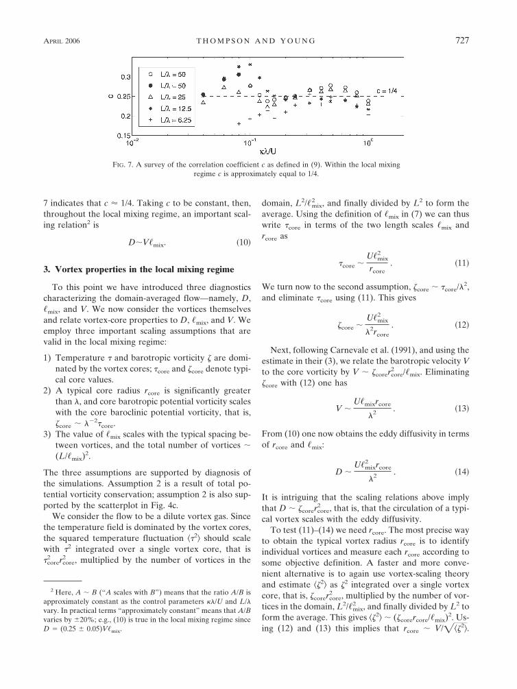
7 indicates that c � 1/4. Taking c to be constant, then,throughout the local mixing regime, an important scal-ing relation2 is

D�V�mix. 10�

3. Vortex properties in the local mixing regime

To this point we have introduced three diagnosticscharacterizing the domain-averaged flow—namely, D,�mix, and V. We now consider the vortices themselvesand relate vortex-core properties to D, �mix, and V. Weemploy three important scaling assumptions that arevalid in the local mixing regime:

1) Temperature � and barotropic vorticity � are domi-nated by the vortex cores; �core and �core denote typi-cal core values.

2) A typical core radius rcore is significantly greaterthan �, and core barotropic potential vorticity scaleswith the core baroclinic potential vorticity, that is,�core � ��2�core.

3) The value of �mix scales with the typical spacing be-tween vortices, and the total number of vortices �(L/�mix)2.

The three assumptions are supported by diagnosis ofthe simulations. Assumption 2 is a result of total po-tential vorticity conservation; assumption 2 is also sup-ported by the scatterplot in Fig. 4c.

We consider the flow to be a dilute vortex gas. Sincethe temperature field is dominated by the vortex cores,the squared temperature fluctuation ��2 should scalewith �2 integrated over a single vortex core, that is�2

corer2core, multiplied by the number of vortices in the

domain, L2/�2mix, and finally divided by L2 to form the

average. Using the definition of �mix in (7) we can thuswrite �core in terms of the two length scales �mix andrcore as

�core �U�mix

2

rcore. 11�

We turn now to the second assumption, �core � �core/�2,and eliminate �core using (11). This gives

�core �U�mix

2

�2rcore

. 12�

Next, following Carnevale et al. (1991), and using theestimate in their (3), we relate the barotropic velocity Vto the core vorticity by V � �corer2

core/�mix. Eliminating�core with (12) one has

V �U�mixrcore

�2 . 13�

From (10) one now obtains the eddy diffusivity in termsof rcore and �mix:

D �U�mix

2 rcore

�2 . 14�

It is intriguing that the scaling relations above implythat D � �corer2

core, that is, that the circulation of a typi-cal vortex scales with the eddy diffusivity.

To test (11)–(14) we need rcore. The most precise wayto obtain the typical vortex radius rcore is to identifyindividual vortices and measure each rcore according tosome objective definition. A faster and more conve-nient alternative is to again use vortex-scaling theoryand estimate ��2 as �2 integrated over a single vortexcore, that is, �corer2

core, multiplied by the number of vor-tices in the domain, L2/�2

mix, and finally divided by L2 toform the average. This gives ��2 � (�corercore/�mix)2. Us-ing (12) and (13) this implies that rcore � V/��2.

2 Here, A � B (“A scales with B”) means that the ratio A/B isapproximately constant as the control parameters ��/U and L/�vary. In practical terms “approximately constant” means that A/Bvaries by �20%; e.g., (10) is true in the local mixing regime sinceD � (0.25 � 0.05)V�mix.

FIG. 7. A survey of the correlation coefficient c as defined in (9). Within the local mixingregime c is approximately equal to 1/4.


These considerations motivate the definition of a newlength �� as

�� V2

��2, 15�

and the scaling hypothesis

rcore � ��. 16�

Here �� is simply an easily diagnosed surrogate for rcore.Invoking (16), we can replace rcore by �� in (11)–(14).

In particular from (13) the vortex-scaling theory pre-dicts that the ratio

�1 �V�2

U�mix��

��2��2

��217�

is constant. We see in Fig. 8a that this ratio is indeedremarkably constant although there is variation in thevalue of �1 because of resolution differences (for fur-ther discussion see section 7). These variations do nothave a large effect on our estimates for D in the fol-lowing sections, and for the purposes of making quan-titative estimates we will take �1 to be approximately0.60 (the L/� � 25 and 50 series). Another indication ofthe vortex gas scaling is that the ratio

�2 � ��

��2��218�

is also roughly constant and equal to 0.53, independentof resolution effects; see Fig. 8b.

To further verify our vortex-scaling theory, we use anautomated “vortex census” to quantify vortex statisticsin simulations at seven different values of ��/U. In Fig.9 we provide confirmation of the two relationshipsprominently involving the length scales �mix and rcore. InFig. 9a, we plot the mean number of vortices, N, foreach value of ��/U. Here, N is determined from 50snapshots of the barotropic vorticity field in its equili-brated turbulent state. Vortex theory predicts �mix �N�1/2 and our vortex census shows that �mix �N�0.57�0.05. The variation in the exponent is due tochanges in the vortex census parameters. These param-eters and the vortex census algorithm are described inappendix B. Figure 9b plots the ratio l�/rcore, where rcore

is determined from the vortex census. The ratio is con-stant to within �10% although the observed l�/rcore

does systematically increase as ��/U decreases. Thecore radius is difficult to quantify because typical vor-tices only span three to six grid spaces for these large-domain simulations. Still, the results in Figs. 8 and 9

FIG. 8. A survey of the two constant ratios (a) �1 � �2��2/��2 and (b) �1 � ��/��2��2. Here, �1 varies slightly because of resolution differences between L/� series (seesection 7). The dashed lines indicate �1 � 0.60 and �2 � 0.53. The data shown here focus onthe local mixing regime. Results from some simulations are unavailable because ��2 was notcollected in the original suite of simulations.


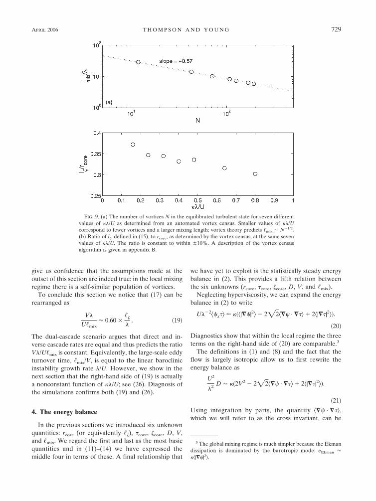
give us confidence that the assumptions made at theoutset of this section are indeed true: in the local mixingregime there is a self-similar population of vortices.

To conclude this section we notice that (17) can berearranged as

V�

U�mix� 0.60

��

�. 19�

The dual-cascade scenario argues that direct and in-verse cascade rates are equal and thus predicts the ratioV�/U�mix is constant. Equivalently, the large-scale eddyturnover time, �mix/V, is equal to the linear baroclinicinstability growth rate �/U. However, we show in thenext section that the right-hand side of (19) is actuallya nonconstant function of ��/U; see (26). Diagnosis ofthe simulations confirms both (19) and (26).

4. The energy balance

In the previous sections we introduced six unknownquantities: rcore (or equivalently ��), �core, �core, D, V,and �mix. We regard the first and last as the most basicquantities and in (11)–(14) we have expressed themiddle four in terms of these. A final relationship that

we have yet to exploit is the statistically steady energybalance in (2). This provides a fifth relation betweenthe six unknowns (rcore, �core, �core, D, V, and �mix).

Neglecting hyperviscosity, we can expand the energybalance in (2) to write

U��2��x� � ��|��|2 � 2�2�� · �� 2�|��|2�.

20�

Diagnostics show that within the local regime the threeterms on the right-hand side of (20) are comparable.3

The definitions in (1) and (8) and the fact that theflow is largely isotropic allow us to first rewrite theenergy balance as

U2

�2 D � �2V2 � 2�2�� · �� 2�|��|2�.

21�

Using integration by parts, the quantity �� · ��,which we will refer to as the cross invariant, can be

3 The global mixing regime is much simpler because the Ekmandissipation is dominated by the barotropic mode: �Ekman ��|��|2.

FIG. 9. (a) The number of vortices N in the equilibrated turbulent state for seven differentvalues of ��/U as determined from an automated vortex census. Smaller values of ��/Ucorrespond to fewer vortices and a larger mixing length; vortex theory predicts �mix � N�1/2.(b) Ratio of l�, defined in (15), to rcore, as determined by the vortex census, at the same sevenvalues of ��/U. The ratio is constant to within �10%. A description of the vortex censusalgorithm is given in appendix B.


rewritten as ��. Both temperature and barotropicvorticity are dominated by values in the vortex cores;therefore, the product �� is strongly dominated by corevalues. Thus, returning to our vortex-core relationsfrom section 3, and specifically using (18) with the defi-nitions of �mix and �� in (7) and (15), we can write

�� 2UV�mix

��

, 22�

where �2 � 0.53. Note that the negative sign is neces-sary on the left-hand side of (22) because � and � arenegatively correlated. This strong anticorrelation be-tween � and � is important because the cross termmakes a significant contribution to the dissipation in(20).

The final term on the right-hand side of (20) involves�|��|2. Unfortunately, �|��|2 cannot be directly relatedto the vortex-core properties because the domain aver-age of the temperature gradient fluctuations is notdominated by vortex cores. Instead, equal contributionsto this average come from the vortex cores and thesurrounding filamentary sea. In the sea between thevortices, � suffers a cascade to small scales and |��| can

become comparable to typical core values. The nonvor-tex contribution to �|��|2 is further enhanced becausethe filamentary sea accounts for a much larger percent-age of the domain than do the vortices.

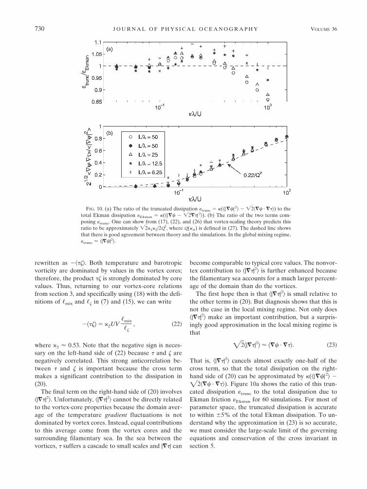
The first hope then is that �|��|2 is small relative tothe other terms in (20). But diagnosis shows that this isnot the case in the local mixing regime. Not only does�|��|2 make an important contribution, but a surpris-ingly good approximation in the local mixing regime isthat

�2�|��|2 � �� · ��. 23�

That is, �|��|2 cancels almost exactly one-half of thecross term, so that the total dissipation on the right-hand side of (20) can be approximated by �(�|��|2 ��2�� · ��). Figure 10a shows the ratio of this trun-cated dissipation �trunc to the total dissipation due toEkman friction �Ekman for 60 simulations. For most ofparameter space, the truncated dissipation is accurateto within �5% of the total Ekman dissipation. To un-derstand why the approximation in (23) is so accurate,we must consider the large-scale limit of the governingequations and conservation of the cross invariant insection 5.

FIG. 10. (a) The ratio of the truncated dissipation �trunc � �(�|��| 2 � �2�� · ��) to thetotal Ekman dissipation �Ekman � �(�|�� 2��| 2). (b) The ratio of the two terms com-posing �trunc. One can show from (17), (22), and (26) that vortex-scaling theory predicts thisratio to be approximately �2�1�2/2Q2, where Q(�*) is defined in (27). The dashed line showsthat there is good agreement between theory and the simulations. In the global mixing regime,�trunc � �|��|2.


Returning to the energy balance in (21), and applyingthe approximations in (22) and (23), we have

U2

�2 D � ��2V2 � �2�2UV�mix

��. 24�

If we first replace D with cV�mix and then multiply (24)by a factor of �3/U3�2

mix, we find that each of the threeterms is proportional to some power of V�/U�mix. From(17), this ratio is equivalent to �1��/�. These steps re-duce (24) to the quadratic equation

2�*��1

��

� �2

� c��1

��

� � � �2�*�1�2 � 0,

25�

where �* � ��/U, the nondimensional bottom friction.Solving (25) and choosing the positive root gives

�1

��

�� Q�*�, 26�

where

Q�*� �12 � c

2�*�� c2

4�2

*� 2�2�1�2�,

�12 � 1

8�*�� 1

64�2

*� 0.9�. 27�

In the second expression the numerical values are ob-tained using c � 0.25, �1 � 0.60, and �2 � 0.53.

The goal is to find a scaling for D, so we return to D� cV�mix, and express V in terms of �� and �mix using(17). With c � 1/4 this leads to

D �U�mix

2

4� ��1

��

� �, 28�

or using (26)

D �U�mix

2

8� � 18�*

�� 1

64�2

*� 0.9�. 29�

A complete expression for D solely in terms of externalparameters requires another relation connecting �mix toknown quantities. Unfortunately, we have not found aphysical argument for this relationship. Instead in sec-tion 6 we propose an empirical fit for �mix. The mainresult obtained from those empirical considerations isthat in the local regime

�mixloc � 4� exp� 3U

10��, 30�

[see (38) and the surrounding discussion]. Eliminating�mix from (29) using (30) gives the energy-balance scal-ing, D � DEB

loc , where

DEBloc � 2 exp� 3

5�*�� 1

8�*�� 1

64�2

*� 0.9�U�.

31�

This equation is the smooth curve in Fig. 1. Further-more, Fig. 5a shows the ratio of the simulated D to DEB

within the local mixing regime. For data within theglobal mixing regime, �mix is set equal to �L in (29).The ratio is close to unity in the local mixing regime,and even does reasonably well in the global mixing re-gime where c, �1, and �2 are variable. Further discus-sion of the transition from local to global mixing ap-pears in section 6.

5. The large-scale limit and the cross invariant

Our analysis of the energy balance equation in sec-tion 4 relies crucially on the approximation (23), whichenables us to relate �|��|2 to vortex properties. To un-derstand this approximation we consider the large-scale, slow-time limit of the equations of motion, that is,the dynamics on length scales much greater than �. Toextract this limit we first nondimensionalize length with� and time with �/U. Then if � � �/�mix 1, one obtainsthe large-scale limit with �x → ��x and �t → ��t. Toretain the proper balance of terms, the amplitudes of �and � are boosted by a factor of 1/�. The result of thismaneuver is the scaled evolution equations:

2�t � J�, 2�� J�, 2�� 2�x � ��*�

2� ��2��

� O�2� 32�

and

�t � J�, �� x � �2��*2�2� � �� O�2�,

33�

where �* � ��/U. The left-hand sides of (32) and (33)are familiar from earlier studies of large-scale quasigeo-strophic turbulence (Salmon 1980; LH95). The right-hand sides of (32) and (33) reveal the large-scale effectsof bottom friction. In (32) the O(��1�*) dissipativeterms on the right are significant, if not dominant, de-pending on the size of �*. Notice also that the largestcoupling of � into (33) is due to bottom friction, ratherthan the O(�2) nonlinear terms.

If �* � O(1), we must have � � �2� � O(�) tocontrol the ��1 term on the right of (32). This is Arbicand Flierl’s (2004a) equivalent barotropic flow, where


the lower layer is almost spun down.4 Roughly speak-ing, � � �2� � O(�) is characteristic of most of thelocal regime. We resisted this conclusion and attemptedto control the ��1 term on the right of (32) by making�* sufficiently small. But this victory is pyrrhic becauseonce �*/� � O(1) the system is in the global regime.Thus, in the local regime, where the concept of an eddydiffusivity is relevant, the bottom friction is alwaysproblematic in the large-scale barotropic vorticity equa-tion in (32). This is a fundamental reason for the failureof the dual-cascade theory.

The nonlinear terms in (32) and (33) conserve thecross invariant:

�� · �� . 34�

The motivation for studying the cross invariant comesfrom the strong anticorrelation between � and � withinthe vortex cores. To obtain the cross-invariant conser-vation law, multiply (32) by � and (33) by � and add theresults. Averaging over space, one finds that to leadingorder

�

�t �� *�

�� · �� 2�|��|2�. 35�

We emphasize that (35) is a new conservation law ofthe large-scale dynamics—there is no clear relation be-tween (35) and the energy and enstrophy conservationlaws of the full system. Now in statistical steady state,there can be no net production of the cross invariant��. This requires that the right-hand side of (35) iszero (or take a time average). This prediction is wellverified in the simulations, and crucial in simplifying

the energy balance equation in section 4 [see (23) andsubsequent discussion].

6. Empirical expressions for the mixing length

To eliminate the mixing length from (29) we need toexpress �mix in terms of external parameters. We areunable to find a satisfactory physical argument and in-stead we indulge in some curve fitting. In Fig. 6b, �mix

has an independent dependence on two dimensionlessparameters, L/� and ��/U. We found empirically thatthe introduction of the combination , defined by

�3

10U

�� ln��L

4� �, 36�

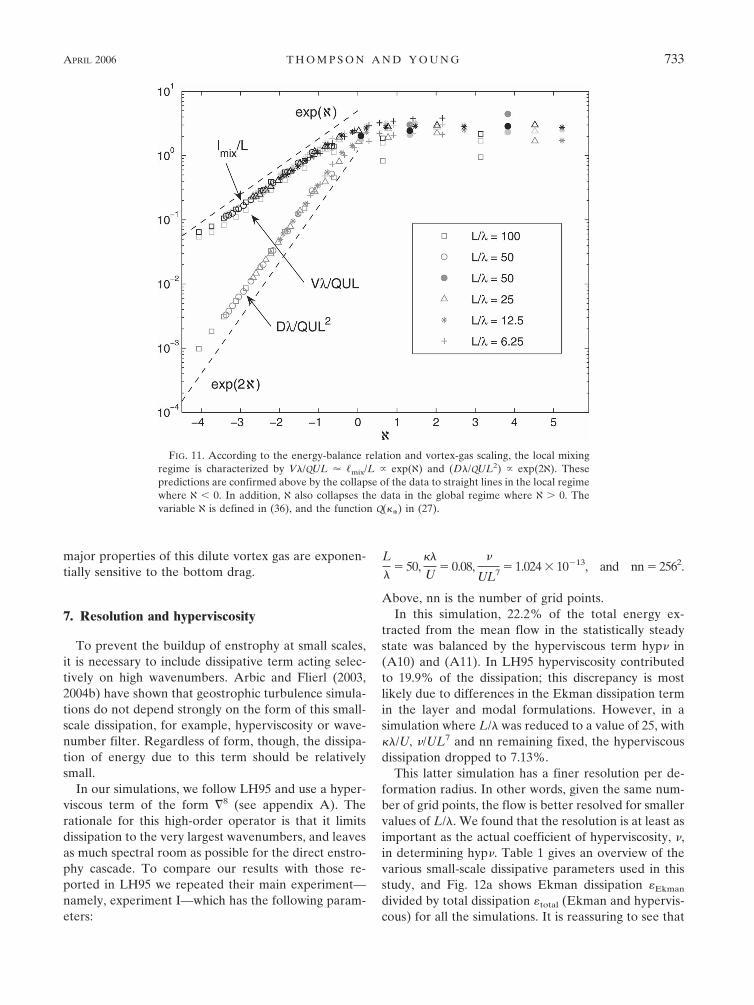
collapses the data in both the local and global regimes(see Fig. 11).

The definition (36) is constructed so that � 0 isroughly the border between local and global mixing.The factor 3/10 is a simple fraction that best collapsesthe �mix data in the local mixing regime. The combina-tion accounts for the observation that for increasingL/�, the global–local transition occurs at smaller andsmaller values of ��/U. However, the dependence isvery weak, and this motivates the logarithm of L/� in(36).

Using , we propose the empirical formula

�mix � �Le

�1 � e2 � �LF �. 37�

Figure 6c shows that (37) collapses the �mix data. Equa-tion (37) is constructed so that

�mix � ��L, in the global regime, e2 � 1,

�L exp � � 4� exp3U�10��, in the local regime, e2 1.38�

In the global mixing regime �mix saturates at �L, orroughly half the domain size. In the local regime �mix isindependent of L and exponentially sensitive to ��/U.

It is our consistent experience that this exponentialdependence of �mix on U/�� is more convincing than apower law in the local regime. For example, the �mix/Lpoints in Fig. 11 fall cleanly on the straight line corre-sponding to e . This observation is the most compellingmotivation for the introduction of e in (37) and (38).

In the local mixing regime the vortex-scaling theoryin (13) and (14) predicts that V � rcore�mix and D

�rcorel2mix. Since rcore � �� Q(�*) we can eliminate thedependence on rcore by considering V/Q and D/Q, whereQ(�*) is defined in (27). Thus, in the local mixing re-gime vortex scaling predicts that

V

Q� �mix � e 39�

and

D

Q� �mix

2 � e2 . 40�

Figure 11 shows the ratios above plotted against . Thestraight lines in the local regime ( � 0) further confirmthe vortex scaling. Figure 11 also shows that all the

4 Notice that if � is precisely proportional to �, then the energyproduction ��x� also precisely vanishes. Thus, the residual � ��2� is certainly nonzero and very important.


major properties of this dilute vortex gas are exponen-tially sensitive to the bottom drag.

7. Resolution and hyperviscosity

To prevent the buildup of enstrophy at small scales,it is necessary to include dissipative term acting selec-tively on high wavenumbers. Arbic and Flierl (2003,2004b) have shown that geostrophic turbulence simula-tions do not depend strongly on the form of this small-scale dissipation, for example, hyperviscosity or wave-number filter. Regardless of form, though, the dissipa-tion of energy due to this term should be relativelysmall.

In our simulations, we follow LH95 and use a hyper-viscous term of the form �8 (see appendix A). Therationale for this high-order operator is that it limitsdissipation to the very largest wavenumbers, and leavesas much spectral room as possible for the direct enstro-phy cascade. To compare our results with those re-ported in LH95 we repeated their main experiment—namely, experiment I—which has the following param-eters:

L

�� 50,

��

U� 0.08,

�

UL7 � 1.024 10�13, and nn � 2562.

Above, nn is the number of grid points.In this simulation, 22.2% of the total energy ex-

tracted from the mean flow in the statistically steadystate was balanced by the hyperviscous term hyp� in(A10) and (A11). In LH95 hyperviscosity contributedto 19.9% of the dissipation; this discrepancy is mostlikely due to differences in the Ekman dissipation termin the layer and modal formulations. However, in asimulation where L/� was reduced to a value of 25, with��/U, �/UL7 and nn remaining fixed, the hyperviscousdissipation dropped to 7.13%.

This latter simulation has a finer resolution per de-formation radius. In other words, given the same num-ber of grid points, the flow is better resolved for smallervalues of L/�. We found that the resolution is at least asimportant as the actual coefficient of hyperviscosity, �,in determining hyp�. Table 1 gives an overview of thevarious small-scale dissipative parameters used in thisstudy, and Fig. 12a shows Ekman dissipation �Ekman

divided by total dissipation �total (Ekman and hypervis-cous) for all the simulations. It is reassuring to see that

FIG. 11. According to the energy-balance relation and vortex-gas scaling, the local mixingregime is characterized by V�/QUL � �mix/L � exp( ) and (D�/QUL2) � exp(2 ). Thesepredictions are confirmed above by the collapse of the data to straight lines in the local regimewhere � 0. In addition, also collapses the data in the global regime where � 0. Thevariable is defined in (36), and the function Q(�*) in (27).


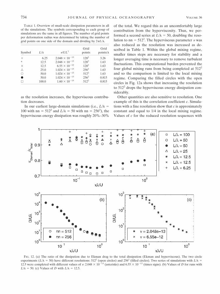
as the resolution increases, the hyperviscous contribu-tion decreases.

In our earliest large-domain simulations (i.e., L/� �100 with nn � 5122 and L/� � 50 with nn � 2562), thehyperviscous energy dissipation was roughly 20%–30%

of the total. We regard this as an uncomfortably largecontribution from the hyperviscosity. Thus, we per-formed a second series at L/� � 50, doubling the reso-lution to nn � 5122. The hyperviscous parameter � wasalso reduced as the resolution was increased as de-scribed in Table 1. Within the global mixing regime,smaller times steps are necessary for stability and alonger averaging time is necessary to remove turbulentfluctuations. This computational burden prevented thefour global mixing runs from being completed at 5122

and so the comparison is limited to the local mixingregime. Comparing the filled circles with the opencircles in Fig. 12a shows that increasing the resolutionto 5122 drops the hyperviscous energy dissipation con-siderably.

Other quantities are also sensitive to resolution. Oneexample of this is the correlation coefficient c. Simula-tions with a fine resolution show that c is approximatelyconstant and equal to 1/4 in the local mixing regime.Values of c for the reduced resolution sequences with

FIG. 12. (a) The ratio of the dissipation due to Ekman drag to the total dissipation (Ekman and hyperviscous). The two circleexperiments (L/� � 50) have different resolutions: 5122 (open circles) and 2562 (filled circles). Two series of simulations with L/� �12.5 were completed with different values of �: 2.048 10�13 (asterisks) and 6.55 10�12 (times signs). (b) Values of D for runs withL/� � 50. (c) Values of D with L/� � 12.5.

TABLE 1. Overview of small-scale dissipation parameters in allof the simulations. The symbols corresponding to each group ofsimulations are the same in all figures. The number of grid pointsper deformation radius was determined by taking the number ofgrid points on one side of the domain and dividing by 2�L/�.

Symbol L/� �/UL7Grid

pointsGrid

points/�

� 6.25 2.048 10�13 1282 3.26* 12.5 2.048 10�13 1282 1.63 12.5 6.55 10�12 1282 1.63� 25.0 1.024 10�13 2562 1.63� 50.0 1.024 10�13 5122 1.63� 50.0 1.024 10�13 2562 0.815� 100.0 1.60 10�15 5122 0.815


L/� � 100 and 50 collapsed onto a single curve withvalues between 0.27 and 0.37 in the local regime (notshown). This systematic variation due to insufficientresolution was limited to data within the local mixingregime. This led us to omit data for simulations withL/� � 100 for some plots. Also, in Fig. 8a, ��2 is shownto be sensitive to simulation resolution.

Considering the effect resolution has on hyp�, c, �1,and other properties, it is somewhat surprising thatvarying resolution makes only a small change in D.Figure 12b compares the values of D for the two serieswith L/� � 50. All the simulations in the local mixingregime have been performed at both resolutions, andthe values of D are so similar that it is difficult to dis-tinguish the filled circles from the open circles in Fig.12b. This result gives us confidence in our L/� � 100results for D despite the large hyperviscous energy dis-sipation in this sequence (Fig. 12a).

As a further test, Fig. 12c shows that varying � atfixed resolution has a small effect on D. Figure 12cshows two sequences (marked with asterisks and timessigns, respectively) with L/� � 12.5 and � � 32�*, withnn � 1282 in both cases. Again, the large change in �has little impact on D, especially in the local mixingregime. In the global regime, there is a systematic de-crease in D for the simulations with increased hyper-viscosity. This discrepancy may be due to the fact thatthe simulations with increased � spin up faster, and arealso less volatile.

8. Discussion and conclusions

In this article we have shown that the main predic-tions of the dual-cascade theory of equilibrated baro-clinic turbulence on an f plane are inaccurate; for ex-ample, the ratios Dk0

2�/U and V�/U�mix are not con-stant. We have identified the underlying physicalreasons for the failure of this theory, for example, thedominance of bottom drag in the large-scale barotropicvorticity equation in (32), and the prominence of co-herent vortices. We have proposed an alternativetheory for baroclinic eddy fluxes based on vortex-gasscaling (Carnevale et al. 1991) and energy balance. Ani-mations of equilibrated simulations show that vorticespersist and travel across the domain. The baroclinicheat flux is evident in these animations as a systematictendency for hot anticyclonic vortices to move north-ward, and cold cyclonic vortices southward. However, agreat difference from the barotropic problem studiedby Carnevale et al. (1991) is that in the equilibratedstate same-signed vortex merger is rare.

An important feature of the vortex theory is thatthere are at least four relevant length scales. In the localregime these four adhere to the relationships

� � rcore �mix L. 41�

Scale separation between L and �mix is necessary for thevalidity of diffusive parameterizations, but there is alsoan important scale separation between �mix and rcore. Insection 3, we showed that the diffusivity D depends onboth the mixing length and the core radius through

D �U�mix

2 rcore

�2 . 42�

In section 4, the mechanical energy Eq. (2) is used toexpress �� (and therefore rcore) in terms of ��/U; forexample, see (26). And in section 6 we proposed anempirical expression for �mix in terms of ��/U; for ex-ample, see (38). The exponential sensitivity of �mix to��/U enters through this empirical relation, but a com-pelling physical explanation for this exponential rela-tion has eluded us. We believe that the answer is againrelated to the long-lived coherent vortices that domi-nate the flow. A full understanding of homogeneousquasigeostrophic turbulence on an f plane will requirean analysis of how these coherent structures are cre-ated, how they work to halt the linear baroclinic insta-bility, and how they interact in statistical equilibrium.

Of course, introduction of a planetary potential vor-ticity gradient, �, would make this model more appli-cable to the ocean and also provide a mechanism forhalting, without damping, the inverse cascade and sup-pressing vortices. Held and Larichev (1996) and Lap-eyre and Held (2003) have shown that � can indeed haltthe inverse cascade, and they have presented scalingsfor the diffusive flux again applying the dual-cascademodel. Danilov and Gurarie (2002) have presentedbarotropic simulations that include both bottom fric-tion and �, and have documented a transition betweenfriction-dominated and �-dominated regimes. Still, anunderstanding of how these two mechanisms influencethe eddy fluxes and the formation of coherent struc-tures is incomplete. This will be one focus of a forth-coming study based on a new suite of simulations thatinclude the effects of � and bottom friction. Preliminaryresults suggest that coherent structures can be promi-nent features even in simulations with moderate valuesof �. Thus, the work presented here lays a foundationfor understanding the role of coherent structures andeddy fluxes that will apply to more realistic models.

Acknowledgments. We thank Lien Hua and PatriceKlein for providing the spectral code used in this work.We have benefited from conversations with PaolaCessi, Stefan Llewellyn Smith, Rick Salmon, and GeoffVallis. Comments from K. Shafer Smith and an anony-mous reviewer significantly improved the presentation.


This work was supported by the National ScienceFoundation under the Collaborations in Mathemati-cal Geo sciences initiative (Grants ATM0222109 andATM0222104). AFT also gratefully acknowledges thesupport of an NDSEG Fellowship.

APPENDIX A

The Two-Mode Equations of Motion

The derivation of the modal equations used in ourstudy is based on Flierl (1978), and also includes forcingterms that arise when there is a mean shear in the basicstate as discussed in Hua and Haidvogel (1986). Ourequations differ from those of Hua and Haidvogel onlyin the form of the hyperviscous term, which is used toabsorb enstrophy cascading to the highest wavenum-bers. The main difference between the modal decom-position used here and the method used by Larichevand Held (1995) appears in the coefficients of the bot-tom drag term as shown below.

The continuous quasigeostrophic equations are writ-ten as

�

�tQ � J�, Q� � ��8Q. A1�

Here J represents the Jacobian, J(a, b) � axby � aybx, �is the streamfunction such that u � ��y and � � �x,and

Q � 2� � f�N�2�zz A2�

is the potential vorticity. We consider dynamics on an fplane, and take the Brunt–Väisälä frequency N to beconstant. The coefficient of hyperviscosity is given by �and H is the depth of the ocean. We then define the firstRossby radius of deformation as

� �NH

�. A3�

Using a truncated modal expansion in the vertical, weconsider the barotropic and first baroclinic modes inthe presence of a mean shear. We write this as

�x, y, z, t� � �x, y, t�

� �Uy � �x, y, t�!�2 cos��z

H �,

A4�

where � and � are the perturbation streamfunctions ofthe barotropic and baroclinic modes, respectively. Thefactor of �2 arises from normalization of the modes(Flierl 1978). The potential vorticity written in terms ofthis modal expansion is

Q � 2� � 2� � ��2� � U��2y��2 cos��z

H �.

A5�

We now apply the modal decomposition of � to thequasigeostrophic equation and project in the barotropicand baroclinic modes. The frictional, or Ekman drag,terms arise from the bottom boundary condition:

wx, y, �H, t� � �E2�x, y, �H, t�, A6�

where "E is the Ekman layer depth. In our model theEkman drag coefficient is defined by � � f"E/H.

The modal equations are

2�t � J�, 2�� J�, 2�� U2�x � ��2� ��2�� 82��

A7�

and

2 � ��2��t � J �, 2 � ��2��! � J�, 2��

� U2 � ��2��x � ��22� � �2��

� �8�2 � ��2��.

A8�

Nondimensionalizing lengths with the deformationlength � and time with �/U gives the three nondimen-sional parameters in the system:

�

L,��

U, and

�

U�7 . A9�

The energy balance is obtained in the standard mannerby multiplying the barotropic and baroclinic modalequations by � and �, respectively, and ensemble aver-aging. In a statistically steady state the energy balancerequires

U��2��x� � ��|�� 2��|2 � hyp�,

A10�

where the hyperviscous term is given by

hyp� � ��|4�|2 � ��|4�|2 � ��2�4��2.

A11�

APPENDIX B

Vortex Census Algorithm

The automated vortex census algorithm primarilyfollows the method outlined in McWilliams (1990) toidentify vortices in a two-dimensional gridded vorticityfield at a given time. The method begins by identifying


all points above a vorticity threshold value �min. Fol-lowing McWilliams (1990), this value is taken to be 5%of the maximum vorticity magnitude in the field. Thevortices are also required to have a vorticity extrema attheir centers. Thus, any point whose magnitude issmaller than one or more of its surrounding points isalso excluded. Because we are interested in countingaxisymmetric structures, we added a further constraintbased on the Okubo–Weiss parameter (Okubo 1970,Weiss 1991), which measures the relative importance ofvorticity versus strain. The Okubo–Weiss parameter is

OW � sn2 � ss

2 � �2 � 4ux2 � uy�x�, B1�

where sn � ux � �y is the normal component of strainand ss � uy � �x is the shear component of strain. TheOkubo–Weiss parameter is negative when rotationdominates and positive when strain dominates. There-fore, we require that the Okubo–Weiss parameter atthe center of each of our vortices be negative and havea magnitude larger than a threshold OWmin. Similar tothe vorticity we take OWmin to be 5% of the maximumOW magnitude in the field (the value of OW at thepoint of maximum magnitude is always negative).

The boundary of each vortex is determined followingthe method in McWilliams (1990), which traces a coun-terclockwise path around the boundary based on a vor-ticity threshold. Using the boundary to measure rcore

proved to be difficult since not all vortices are perfectlyaxisymmetric and many vortices only have a core radiusof three to four grid points. We found that a moreeffective method for determining an average vortex ra-dius was to count all the points that had a negativevalue of OW and a magnitude greater than OWmin.Considering the physical fields, these points were foundto lie almost exclusively inside the vortex cores. Divid-ing the number of points that satisfy the OW thresholdby the number of vortices in that particular snapshotprovides an estimate of the area of an average vortex(this is not the true area since we are only countingpoints). From observations of the physical fields, thesquare root of this number was found to agree well witha typical core radius and was taken as the value for rcore

in Fig. 9b.Simulations with L/� � 25 and ��/U � (0.16, 0.24,

0.32, 0.48, 0.64, 0.80) were run for a time tU/� � 125 inthe equilibrated state during which 50 snapshots ofbarotropic vorticity and the Okubo–Weiss parameter ofthe barotropic mode were saved. The vortex census wascompleted for each snapshot and the values for N andrcore plotted in Fig. 9 are the mean of these 50 realiza-tions. The values for �min and OWmin were varied sys-tematically. These changes alter the resulting values of

N and rcore, but the relationship between different val-ues of bottom drag does not change significantly. Forexample, changes in threshold values cause the slope inFig. 9a to vary between �0.52 and �0.62.

REFERENCES

Arbic, B. K., and G. R. Flierl, 2003: Coherent vortices and kineticenergy ribbons in asymptotic, quasi two-dimensional f-planeturbulence. Phys. Fluids, 15, 2177–2189.

——, and ——, 2004a: Baroclinically unstable geostrophic turbu-lence in the limits of strong and weak bottom Ekman friction:Application to midocean eddies. J. Phys. Oceanogr., 34,2257–2273.

——, and ——, 2004b: Effects of mean flow direction on energy,isotropy, and coherence of baroclinically unstable beta-planegeostrophic turbulence. J. Phys. Oceanogr., 34, 77–93.

Carnevale, G. F., J. C. McWilliams, Y. Pomeau, J. B. Weiss, andW. R. Young, 1991: Evolution of vortex statistics in two-dimensional turbulence. Phys. Rev. Lett., 66, 2735–2737.

Danilov, S., and D. Gurarie, 2002: Rhines scale and spectra of the�-plane turbulence with bottom drag. Phys. Rev., 65E,R067301, doi:10.1103/PhysRevE.65.067301.

Flierl, G. R., 1978: Models of vertical structure and the calibrationof two-layer models. Dyn. Atmos. Oceans, 2, 342–381.

Green, J. S. A., 1970: Transfer properties of the large-scale eddiesand the general circulation of the atmosphere. Quart. J. Roy.Meteor. Soc., 96, 157–185.

Haidvogel, D. B., and I. M. Held, 1980: Homogeneous quasigeo-strophic turbulence driven by a uniform temperature gradi-ent. J. Atmos. Sci., 37, 2644–2660.

Held, I. M., and V. D. Larichev, 1996: A scaling theory for hori-zontally homogeneous, baroclinically unstable flow on a betaplane. J. Atmos. Sci., 53, 946–952.

Hua, B. L., and D. B. Haidvogel, 1986: Numerical simulations ofthe vertical structure of quasi-geostrophic turbulence. J. At-mos. Sci., 43, 2923–2936.

Lapeyre, G., and I. M. Held, 2003: Diffusivity, kinetic energy dis-sipation, and closure theories for the poleward eddy heatflux. J. Atmos. Sci., 60, 2907–2916.

Larichev, V., and I. Held, 1995: Eddy amplitudes and fluxes in ahomogeneous model of fully developed baroclinic instability.J. Phys. Oceanogr., 25, 2285–2297.

McWilliams, J. C., 1990: The vortices of two-dimensional turbu-lence. J. Fluid Mech., 219, 361–385.

Okubo, A., 1970: Horizontal dispersion of floatable particles inthe vicinity of velocity singularities such as convergences.Deep-Sea Res., 17, 445–454.

Pavan, V., and I. M. Held, 1996: The diffusive approximation foreddy fluxes in baroclinically unstable jets. J. Atmos. Sci., 53,1262–1272.

Pedlosky, J., 1983: The growth and decay of finite-amplitude baro-clinic waves. J. Atmos. Sci., 40, 1863–1876.

Rhines, P. B., 1977: The dynamics of unsteady currents. The Sea,E. A. Goldberg et al., Eds., Marine Modeling, Vol. 6, Wileyand Sons, 189–318.

Riviere, P., and P. Klein, 1997: Effects of an asymmetric frictionon the nonlinear equilibration of a baroclinic system. J. At-mos. Sci., 54, 1610–1627.


——, A. M. Treguier, and P. Klein, 2004: Effects of bottom fric-tion on nonlinear equilibration of an oceanic baroclinic jet. J.Phys. Oceanogr., 34, 416–432.

Salmon, R., 1978: Two-layer quasigeostrophic turbulence in asimple special case. Geophys. Astrophys. Fluid Dyn., 10, 25–52.

——, 1980: Baroclinic instability and geostrophic turbulence.Geophys. Astrophys. Fluid Dyn., 15, 167–211.

Smith, K. S., and G. K. Vallis, 2002: The scales and equilibrationof midocean eddies: Forced-dissipative flow. J. Phys. Ocean-ogr., 32, 1699–1720.

Stone, P. H., 1972: A simplified radiative-dynamical model for thestatic stability of rotating atmospheres. J. Atmos. Sci., 29,11–37.

Weiss, J., 1991: The dynamics of enstrophy transfer in two-dimensional hydrodynamics. Physica D, 48, 273–294.


scaling baroclinic eddy fluxes: vortices and energy balance · scaling baroclinic eddy fluxes:...

Documents