tunnelling and underground space technology - geo...

Tunnelling and Underground Space Technology 25 (2010) 188–197

Contents lists available at ScienceDirect

Tunnelling and Underground Space Technology

journal homepage: www.elsevier .com/ locate / tust

Review

Comparative evaluation of methods to determine the earth pressure distributionon cylindrical shafts: A review

Tatiana Tobar, Mohamed A. Meguid *

Department of Civil Engineering and Applied Mechanics, McGill University, 817 Sherbrooke Street West, Montreal, Quebec, Canada H3A 2K6

a r t i c l e i n f o a b s t r a c t

Article history:Received 22 April 2009Received in revised form 15 October 2009Accepted 5 November 2009Available online 4 December 2009

Keywords:Cylindrical shaftsEarth pressure theoryPhysical modelingSoil–structure interaction

0886-7798/$ - see front matter � 2009 Elsevier Ltd. Adoi:10.1016/j.tust.2009.11.001

* Corresponding author. Tel.: +1 514 398 1537; faxE-mail addresses: [email protected]

[email protected] (M.A. Meguid).

Various methods used for calculating and measuring the earth pressure distribution on cylindrical shaftsconstructed in sand are evaluated. Emphasis is placed on a comparison between the calculated earthpressure using different methods for given sand and wall conditions. The effects of the assumptions madein developing these solutions on the pressure distribution are discussed. Physical modeling techniquesused to simulate the interaction between vertical shafts and the surrounding soil are presented. The earthpressure measured and the wall movements required to establish active condition are assessed. Depend-ing on the adopted method of analysis, the calculated earth pressure distribution on a vertical shaft liningmay vary considerably. For shallow shafts, the theoretical solutions discussed in this study provide con-sistent estimates of the active earth pressure. As the shaft depth exceeds its diameter, the solutionsbecome more sensitive to the ratio between the vertical and horizontal arching and only a range of earthpressure values can be obtained. No agreement has been reached among researchers as to the magnitudeof wall movement required to establish active conditions around shafts and further investigations aretherefore needed.

� 2009 Elsevier Ltd. All rights reserved.

Contents

1. Introduction . . . . . . . . . . . . . . . . . . . . . . . . . . . . . . . . . . . . . . . . . . . . . . . . . . . . . . . . . . . . . . . . . . . . . . . . . . . . . . . . . . . . . . . . . . . . . . . . . . . . . . . . . 1882. Theoretical methods. . . . . . . . . . . . . . . . . . . . . . . . . . . . . . . . . . . . . . . . . . . . . . . . . . . . . . . . . . . . . . . . . . . . . . . . . . . . . . . . . . . . . . . . . . . . . . . . . . . 189

2.1. Analytical solutions . . . . . . . . . . . . . . . . . . . . . . . . . . . . . . . . . . . . . . . . . . . . . . . . . . . . . . . . . . . . . . . . . . . . . . . . . . . . . . . . . . . . . . . . . . . . . . 1892.2. Limit equilibrium . . . . . . . . . . . . . . . . . . . . . . . . . . . . . . . . . . . . . . . . . . . . . . . . . . . . . . . . . . . . . . . . . . . . . . . . . . . . . . . . . . . . . . . . . . . . . . . 1902.3. Slip line method . . . . . . . . . . . . . . . . . . . . . . . . . . . . . . . . . . . . . . . . . . . . . . . . . . . . . . . . . . . . . . . . . . . . . . . . . . . . . . . . . . . . . . . . . . . . . . . . 1902.4. Comparison between different theoretical solutions . . . . . . . . . . . . . . . . . . . . . . . . . . . . . . . . . . . . . . . . . . . . . . . . . . . . . . . . . . . . . . . . . . . 192

3. Experimental investigations . . . . . . . . . . . . . . . . . . . . . . . . . . . . . . . . . . . . . . . . . . . . . . . . . . . . . . . . . . . . . . . . . . . . . . . . . . . . . . . . . . . . . . . . . . . . 192
3.1. Shaft sinking . . . . . . . . . . . . . . . . . . . . . . . . . . . . . . . . . . . . . . . . . . . . . . . . . . . . . . . . . . . . . . . . . . . . . . . . . . . . . . . . . . . . . . . . . . . . . . . . . . . 1923.2. Temporary stabilization using fluid pressure . . . . . . . . . . . . . . . . . . . . . . . . . . . . . . . . . . . . . . . . . . . . . . . . . . . . . . . . . . . . . . . . . . . . . . . . . 1933.3. Mechanically adjustable lining . . . . . . . . . . . . . . . . . . . . . . . . . . . . . . . . . . . . . . . . . . . . . . . . . . . . . . . . . . . . . . . . . . . . . . . . . . . . . . . . . . . . . 1943.4. Discussion of experimental investigations. . . . . . . . . . . . . . . . . . . . . . . . . . . . . . . . . . . . . . . . . . . . . . . . . . . . . . . . . . . . . . . . . . . . . . . . . . . . 196
4. Conclusions. . . . . . . . . . . . . . . . . . . . . . . . . . . . . . . . . . . . . . . . . . . . . . . . . . . . . . . . . . . . . . . . . . . . . . . . . . . . . . . . . . . . . . . . . . . . . . . . . . . . . . . . . . 197Acknowledgements . . . . . . . . . . . . . . . . . . . . . . . . . . . . . . . . . . . . . . . . . . . . . . . . . . . . . . . . . . . . . . . . . . . . . . . . . . . . . . . . . . . . . . . . . . . . . . . . . . . 197References . . . . . . . . . . . . . . . . . . . . . . . . . . . . . . . . . . . . . . . . . . . . . . . . . . . . . . . . . . . . . . . . . . . . . . . . . . . . . . . . . . . . . . . . . . . . . . . . . . . . . . . . . . 197

1. Introduction

Vertical shafts are widely used as temporary or permanentearth retaining structures for different engineering applications

ll rights reserved.

: +1 514 398 7361.ill.ca (T. Tobar), mohamed.

(e.g. tunnels, pumping stations and hydroelectric projects). Deter-mining the earth pressure acting on the shaft lining system isessential to a successful design. Classical earth pressure theoriesdeveloped by Coulomb (1776) and Rankine (1857) have been oftenused to estimate earth pressure on shaft walls. These theories wereoriginally developed for infinitely long walls under plane strainconditions. Terzaghi (1920) investigated the effect of wall move-ment on the magnitude of earth pressure acting on a rigid retaining

http://dx.doi.org/10.1016/j.tust.2009.11.001

mailto:[email protected]

mailto:mohamed. [email protected]

mailto:mohamed. [email protected]

http://www.sciencedirect.com/science/journal/08867798

http://www.elsevier.com/locate/tust

Nomenclature

a shaft radiusc soil cohesionDr relative densityF radial forceg gravitational constant of the earthGs specific gravityh excavation depth measured from ground surfaceH shaft wall heightK coefficient of lateral earth pressure on circumferential

planes, K = rh/rv

Ka coefficient of earth pressure at active conditions,Ka = tan2ð45� /=2Þ

Ko coefficient of earth pressure at restKr coefficient of earth pressure for cylindrical shaftsmr normalized earth pressure, mr = p/caN = N/= tan2ð45þ /=2Þn1 normalized extent of the yield zone, n1 = r/aP = p lateral earth pressurepa active earth pressurePo lateral earth pressure at S = 0 mmP1 earth pressure force per unit length of the shaft

circumference

q external surcharger radial distanceS radial displacement at shaft wall or radial soil move-

ment at soil-wall interfaceT tangential forceW weight of the soil wedge

Greek symbolsa inclination of the failure surfaceb angle between the reaction Q acting on the sliding body

and the normald soil unit weight/ friction anglek coefficient of lateral earth pressure on radial planes,

(k = rh/rv)r1, r2, r3 major, intermediate and minor principal stressesrr radial stressrh tangential stressrv vertical stress/� reduced angle of internal friction, /� = / – 5�

T. Tobar, M.A. Meguid / Tunnelling and Underground Space Technology 25 (2010) 188–197 189

wall. He concluded that for dense sand, a wall movement of about0.1% of the wall height is necessary to reach the theoretical activeearth pressure. Following from the work of Terzaghi (1920), exten-sive earth pressure research has been conducted (Terzaghi, 1934,1953; Rowe, 1969; Bros, 1972; Sherif et al., 1982, 1984) to deter-mine the wall displacement required for establishing the activestress state under two-dimensional conditions.

Several theoretical methods have been proposed for the calcula-tion of the active earth pressure on cylindrical retaining walls sup-porting granular material (e.g. Berezantzev, 1958; Prater, 1977).However, the earth pressure distribution obtained using thesemethods was found to vary significantly. In addition, the requiredwall movement to reach the calculated pressures is yet to beunderstood.

Physical models have been used to measure the changes inearth pressure due to the installation of model shafts in granularmaterial under normal gravity conditions or in a centrifuge. Oneof the key challenges in developing a model shaft is to simulatethe radial movement of the supported soil during construction.Researchers have developed different innovative techniques tocapture these features either during or after the installation of aninstrumented lining.

The objective of this study is to review some of the theoreticaland experimental techniques to investigate the active earth pres-sure on cylindrical shaft linings installed in cohesionless ground.The assumptions made in developing different theoretical solu-tions and their effects on the calculated earth pressure are exam-ined. Finally, a comparison is presented between differentphysical modeling techniques used to study the interaction be-tween a shaft lining and the surrounding soil, and the measuredearth pressure distributions are reproduced.

2. Theoretical methods

When Coulomb (1776) and Rankine (1857) developed theirtwo-dimensional earth pressure theories, they also establishedtwo simple methods of analysis: the limit equilibrium and the slipline method. Both methods are based on plastic equilibrium, how-ever they differ in how the solution is obtained. The limit equilib-rium method assumes a suitable failure surface, and basic statics is

used to solve for the earth pressure. Conversely, the slip line meth-od assumes the entire soil mass to be on the verge of failure, andthe solution is obtained through a set of differential equationsbased on plastic equilibrium. Several attempts have been madeto extend these methods to study the active earth pressure againstcylindrical shafts in cohesionless media. Westergaard (1941) andTerzaghi (1943), proposed analytical solutions; Prater (1977) usedthe limit equilibrium method; and Berezantzev (1958), Cheng andHu (2005), Cheng et al. (2007), Liu and Wang (2008), Liu et al.(2009) used the slip line method. In contrast to the classical earthpressure theories, where the active earth pressure calculated usingthe Coulomb or Rankine method are essentially the same, the dis-tributions obtained for axisymmetric conditions may differ consid-erably depending on the chosen method of analysis, as discussedbelow.

2.1. Analytical solutions

The earliest effort to investigate the state of stress around acylindrical opening in soil was made by Westergaard (1941),who studied the stress conditions around small unlined drilledholes, based on the equilibrium of a slipping soil wedge. Terzaghi(1943) extended Westergaard’s theory to large lined holes, thusproposed a method to calculate the minimum earth pressure ex-erted by cohesionless soil on vertical shafts liners. He determinedthe equilibrium of the sliding soil mass assuming rh = rv = r1 andrr = r3 inside the elastic zone and employing the Mohr–Coulombyield criterion. Terzaghi obtained Eqs. (1)–(3) below for the lateralearth pressure on a shaft lining. As stated in Eq. (3), Terzaghi pro-posed the use of a reduced angle of internal friction of the sand, /�,to account for the effect of the nonzero shear stresses in thesolution.

mr ¼ha

N/ þ 12N/

N/ � ðN/ � 2Þn21

N/ þ nN/þ11

ð1Þ

tan /� ¼ n21 � 1

mrnN/

1

� 2N/

N/ þ 1ah

nN/þ11 � 1

nN/

1

ð2Þ

/� ¼ /� 5� ð3Þ

190 T. Tobar, M.A. Meguid / Tunnelling and Underground Space Technology 25 (2010) 188–197

where mr = p/ca, normalized earth pressure; n1 = r/a, normalizedextent of the yield zone; and N/ = tan2 (45 + /�/2); a = shaft radius;h = excavation depth; r = radial distance.

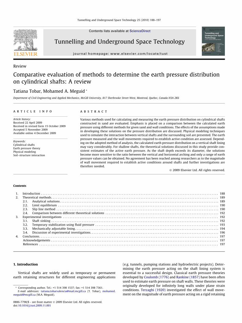
Fig. 1a shows the values of normalized earth pressure, mr, ver-sus normalized depth, h/a, originally computed by Terzaghi (1943)for / = 40� and those computed by the authors for / = 40� and 41�.For / = 40� the difference between the calculated and original datais rather small. Increasing the friction angle from 40� to 41� causesa reduction in the normalized earth pressure by approximately 9%.These numerical values were obtained using the reduced frictionangle given by Eq. (3). The values of mr are computed from Eq.(2) for different assumed values of n1 and the corresponding valuesof h/a are then computed from Eq. (1). The procedure is detailed byTerzaghi (1943).

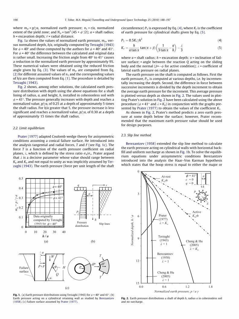
Fig. 2 shows, among other solutions, the calculated earth pres-sure distribution with depth using the above equations for a shaftlining of radius, a, and height, h, installed in cohesionless soil with/ = 41�. The pressure generally increases with depth and reaches anormalized value, p/ca, of 0.25 at a depth of approximately 5 timesthe shaft radius. For h/a greater that 5, the pressure increase is lesssignificant and reaches a normalized value, p/ca, of 0.30 at a depthof approximately 15 times the shaft radius.

2.2. Limit equilibrium

Prater (1977) adapted Coulomb wedge theory for axisymmetricconditions assuming a conical failure surface. He introduced intothe analysis tangential and radial forces, T and F (see Fig. 1c). Theforce T is a function of the earth pressure coefficient on radialplanes, k, which is defined by the stress ratio rh/rv. Prater arguedthat k is a decisive parameter whose value should range betweenKa and Ko and not equal to unity as was implicitly assumed by Ter-zaghi (1943). The earth pressure (force per unit length of the shaft

Fig. 1. (a) Earth pressure distributions using Terzaghi (1943) for / = 40� and 41�. (b)Earth pressure acting on a cylindrical retaining wall as studied by Berezantzev(1958). (c) Failure surface assumed by Prater (1977).

circumference) P1 is expressed by Eq. (4), where Kr is the coefficientof earth pressure for cylindrical shafts given by Eq. (5).

P1 ¼ 0:5Krch2 ð4Þ

Kr ¼h

a tan atanðaþ bÞ 1

3 tan a� a

h

� �� k

3ð5Þ

where a = shaft radius; h = excavation depth; a = inclination of fail-ure surface; = angle between the reaction Q acting on the slidingbody and the normal (b=�/ for active condition); k = coefficient oflateral earth pressure on radial planes.

The earth pressure on the shaft is computed as follows. First theearth pressure, P1, is computed at various depths, i.e. by incremen-tally increasing the depth. Second, the difference in force betweensuccessive increments is divided by the depth increment to obtainthe average earth pressure for the increment. This average pressureis plotted versus depth as shown in Fig. 2. The values used in plot-ting Prater’s solution in Fig. 2 have been calculated using the aboveprocedure (/ = 41� and k = Ko) in conjunction with the graphs pre-sented by Prater (1977) to obtain the values of the coefficient Kr.

As shown in Fig. 2, Prater’s method predicts a zero earth pres-sure at some depth below the surface; however, Prater recom-mended that the maximum earth pressure value should be usedfor design purposes.

2.3. Slip line method

Berezantzev (1958) extended the slip line method to calculatethe earth pressure acting on cylindrical walls with horizontal back-fill and uniform surcharge as shown in Fig. 1b. To solve the equilib-rium equations under axisymmetric conditions Berezantzevintroduced into the analysis the Haar–Von Karman hypothesiswhich states that the hoop stress is equal to either the major or

Fig. 2. Earth pressure distributions a shaft of depth h, radius a in cohesionless soiland no surcharge.


the minor principal stress (Yu, 2006). Thus, under active conditionsBerezantzev assumed that inside the plastic zone the tangentialand radial stresses are equal to the major and minor principalstresses, respectively (rh ¼ rv ¼ r1 and rr ¼ r3). Thus k = rh/rv = 1. To simplify the calculations the slip lines were approxi-mated to straight lines in the vertical direction and the Mohr–Cou-lomb failure criterion was adopted. The governing equations tookthe form of two partial differential equations that he solved usingthe Sokolovski step-by-step computation method. Eq. (6) gives thesimplified form of the solution that evaluates the earth pressure onthe shaft wall as reported by Fujii et al. (1994).

Pa ¼ acffiffiffiffiffiffiKap

g� 11� a

rg�1b

" #þ q

aKa

rgb

!þ cot /

arg

b

!Ka � 1

" #c ð6Þ

where g ¼ 2 tanð/Þ tanð45þ /=2Þ; rb ¼ aþ hffiffiffiffiffiffiKap

; Ka ¼ tan2ð45�/=2Þ; q = external surcharge; c = soil cohesion; a = shaft radius;h = excavation depth.

As shown in Fig. 2, for a shaft of radius, a, in cohesionless soiland no external surcharge, q, the earth pressure distribution basedon Berezantzev is similar to that calculated by Terzaghi, howeverthe maximum pressure is smaller by approximately 40%.

Cheng and Hu (2005) extended Berezantzev’s theory by modify-ing the Haar–Von Karman hypothesis, i.e. k = 1, to develop a moregeneral solution considering a variable earth pressure coefficient, k.An expression for the active earth pressure was proposed as givenbelow.

Fig. 3. Model shaft used in the shaft-sinking method and the meas

Pa ¼ acffiffiffiffiffiffiKap

g� 11� a

rg�1b

!þ q

aKa

rgb

� cot /1� kþ g

g� ae

rgb

Ka

" #c ð7Þ

where g ¼ k tan2 ð45þ /=2Þ � 1; rb ¼ aþ hffiffiffiffiffiffiKap

;e ¼ ð1� kÞg�1 tan2

ð45þ /=2Þ þ 1; 0 < g < 1 and / – 0.Cheng and Hu (2005) found that the case of k = 1 produces the

lowest lateral pressure and therefore a value of k ¼ Ko ¼ ð1� sin /Þwas suggested for engineering applications. The upper and lowerbounds of the lateral earth pressure can then be obtained usingk = Ko and k = 1, respectively, as shown in Fig. 2 (c = 0 and q = 0).

Cheng et al. (2007) and Liu and Wang (2008) introduced addi-tional parameters into the analysis including wall friction, backfillslope, surcharge loads and soil cohesion. Solution of the character-istic equations was obtained numerically leading to a lengthy set ofexpressions that are omitted in this review. The results indicatedthat the pressure distribution is consistently smaller than theone obtained using the simplified solution of Cheng and Hu(2005). Liu and Wang (2008) examined the effect of wall inclina-tion and developed a solution that was essentially similar to thatobtained by Cheng and Hu (2005) simplified solution. They con-cluded that the analytical solution presented by Cheng and Hu pro-vides a reasonable estimate of the active pressure on a verticalshaft for horizontal backfill material and zero wall friction.

Liu et al. (2009) further extended Berezantzev’s theory byassuming a linearly varying k such that it decreases across the plas-tic zone from unity at the shaft circumference to Ko at the elasto-plastic interface. The results obtained based on this method were

ured earth pressure distribution (adapted from Walz (1973)).

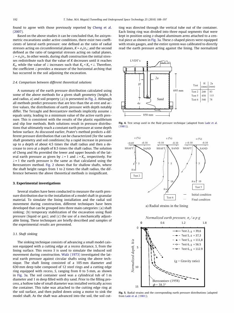
Fig. 4. Test setup used in the fluid pressure technique (adapted from Lade et al.(1981)).


found to agree with those previously reported by Cheng et al.(2007).

Based on the above studies it can be concluded that, for axisym-metric excavations under active conditions, there exist two coeffi-cients of lateral earth pressure: one defined as the ratio of radialstresses acting on circumferential planes, K = rr/rv; and the seconddefined as the ratio of tangential stresses acting on radial planes,k = rh/rv. In other words, during shaft construction the initial stres-ses redistribute such that the value of K decreases until it reachesKa, while the value of k increases such that Ka < Ko < k. Therefore,the coefficient k provides a measure of the horizontal arching thathas occurred in the soil adjoining the excavation.

2.4. Comparison between different theoretical solutions

A summary of the earth pressure distribution calculated usingsome of the above methods for a given shaft geometry (height, hand radius, a) and soil property (/) is presented in Fig. 2. Althoughall methods predict pressures that are less than the at-rest and ac-tive values, the distributions of earth pressure with depth notablydiffer. The Terzaghi and Berezantzev methods implicitly assume kequals unity, leading to a minimum value of the active earth pres-sure. This is consistent with the results of the plastic equilibriumand slip line methods. Both solutions result in pressure distribu-tions that ultimately reach a constant earth pressure at some depthbelow surface. As discussed earlier, Prater’s method predicts a dif-ferent pressure distribution that can be characterized (for the sameshaft geometry and soil conditions) by a rapid increase in pressureup to a depth of about 4.5 times the shaft radius and then a de-crease to zero at a depth of 8.5 times the shaft radius. The solutionof Cheng and Hu provided the lower and upper bounds of the lat-eral earth pressure as given by k = 1 and k = Ko, respectively. Fork = 1 the earth pressure is the same as that calculated using theBerezantzev method. Fig. 2 shows that for shallow shafts, wherethe shaft height ranges from 1 to 2 times the shaft radius, the dif-ference between the above theoretical methods is insignificant.

Fig. 5. Radial strains and the corresponding earth pressure distributions (adaptedfrom Lade et al. (1981)).

3. Experimental investigations

Several studies have been conducted to measure the earth pres-sure distribution due to the installation of a model shaft in granularmaterial. To simulate the lining installation and the radial soilmovement during construction, different techniques have beendeveloped that can be grouped into three main categories: (a) shaftsinking; (b) temporary stabilization of the excavation using fluidpressure (liquid or gas); and (c) the use of a mechanically adjust-able lining. These techniques are briefly described and samples ofthe experimental results are presented.

3.1. Shaft sinking

The sinking technique consists of advancing a small model cais-son equipped with a cutting edge at a recess distance, S, from thelining surface. This recess S is used to simulate the induced soilmovement during construction. Walz (1973) investigated the lat-eral earth pressure against circular shafts using the above tech-nique. The shaft lining consisted of a 105 mm diameter and630 mm deep tube composed of 12 steel rings and a cutting edgering equipped with recess, S, ranging from 0 to 5 mm, as shownin Fig. 3a. The soil container used was a cylindrical tub of 1 mdiameter and 1 m deep filled with dry sand. Prior to the filling pro-cess, a hollow tube of small diameter was installed vertically acrossthe container. This tube was attached to the cutting edge ring atthe soil surface, and then pulled down using a motor to sink themodel shaft. As the shaft was advanced into the soil, the soil cut-

ting was directed through the vertical tube out of the container.Each lining ring was divided into three equal segments that werekept in position using z-shaped aluminum arms attached to a cen-tral piece as shown in Fig. 3a. These z-shaped pieces were equippedwith strain gauges, and the entire system was calibrated to directlyread the earth pressure acting against the lining. The normalized


earth pressure distribution versus normalized depth for S = 0 and2 mm are shown in Fig. 3b. The introduction of the 2 mm recesshas lead to a significant decrease in the measured earth pressurealong the lining, with a maximum reduction of about 75% at h/a = 0.5.

3.2. Temporary stabilization using fluid pressure

In this technique, the soil to be excavated is replaced by a flex-ible rubber bag filled with liquid or gas. The liquid level, or gaspressure, is reduced in stages to simulate the shaft excavation pro-cess. This technique is generally used in centrifuge testing due tothe restrictions in modeling excavation during the test.

Lade et al. (1981) conducted a series of centrifuge tests to inves-tigate the lateral earth pressure against shafts in sand. A cylindricaltub of 850 mm diameter and 695 mm deep was used as the testcontainer in which dry fine Leighton Buzzard sand (c = 15.35–15.5 kN/m3, / = 38.3�) was placed by pluvial deposition. The liningwas formed using a 0.35 mm thick Melinex sheet. The soil insidethe shaft was replaced by two different liquids: ZnCl2-solutionwith density similar to that of the soil and paraffin oil with a den-sity of 7.65 kN/m3. The excavation process was modelled byremoving the liquid in four stages and the liquid level was moni-tored. The readings of eight strain gauge sets installed along thelining were recorded and used to calculate the lateral earth pres-sure. Earth pressure cells and LVDT’s were used to monitor the

Fig. 6. Semi-cylindrical model shaft and earth pressure distribution

stresses around the shaft and the surface settlement, respectively.An overview of the test setup is shown in Fig. 4. The radial strainsin the lining and the normalized earth pressures versus normalizeddepth are reproduced in Fig. 5. Large inward movements at thebase of the fully excavated shaft were recorded which corre-sponded to large pressures at this depth. Before the fluid removal,expansion of the shaft lining was observed due to larger pressuresexerted by the liquid inside the shaft than the outside soil. Similarobservations were made by Kusakabe et al. (1985) in a series ofcentrifuge tests conducted to investigate the influence of axisym-metric excavation on buried pipes. Fig. 5 further shows that themeasured pressures are higher than the calculated using Ber-ezantzev method.

Konig et al. (1991) carried out a series of centrifuge tests tostudy the effects of the shaft face advance on a pre-installed lining.The model shaft consisted of two sections: an upper section madeof rigid tube to simulate the installed lining, and a lower sectionmade of rubber membrane to model the unsupported area of theexcavation. At the initial condition, the membrane was pressurizedwith air to equilibrate the pressure exerted by the soil. To simulatethe shaft face advance, the air pressure was incrementally reduced.The lateral movement of the rubber membrane was monitoredusing LVDT’s embedded in the sand; the stresses in the shaft liningwere monitored using strain gauges installed at different distancesfrom the end of the lining. Results indicated that for dry sand, onlya small support pressure was needed to maintain stability. How-

for smooth and rough walls (adapted from Fujii et al. (1994)).


ever, there was a significant load transfer to the lining closest tothe excavation face due to arching and stress redistribution inthe soil.

3.3. Mechanically adjustable lining

In this technique, a mechanical system is used to move a rigidshaft lining in order to simulate the soil displacement that may oc-cur during the excavation process. Using this technique, it is possi-ble to impose a homogeneous radial displacement along the entireshaft height at a controlled rate. However, the mechanism requiredto model the inward movement of the shaft lining is challenging.

100 cm Motor

Load cells

100 cm

a) Test setup

Fig. 7. Quarter-cylinder model shaft and the earth pressure

Fig. 8. Semi-cylindrical model shaft and the measured earth pressure using a

Researchers have adopted simplified models to simulate the radialdisplacement of the lining (Fujii et al., 1994; Imamura et al., 1999),or took advantage of the radial symmetry to model only a portionof the problem (Herten and Pulsfort, 1999; Chun and Shin, 2006).Tobar and Meguid (2009) developed a mechanical system that al-lowed for the modeling of both the full shaft geometry as well asthe radial displacement of the lining.

Using a mechanically adjustable shaft model, Fujii et al. (1994)conducted centrifuge tests to study the effects of wall friction andsoil displacements on the earth pressure distribution around rigidshafts. The lining was made of an aluminum cylinder of 60 mm indiameter split vertically into two semi-cylinders; one-half was

0

1

2

3

4

50 2 4 6 8 10

S = 0 mm

S = 0.5 mm

Earth pressure (kN/m2)

Nor

mal

ized

dep

th, h

/a

b) Measured earth pressure

distribution (adapted from Herten and Pulsfort (1999)).

shape aspect ratio, H/a, of 4.286 (adapted from Chun and Shin (2006)).


instrumented with small stress transducers and horizontallymoved using a motor to simulate the radial displacement of theshaft lining. Details of the apparatus are shown in Fig. 6a. The mod-el shaft was placed into a rectangular soil container and Toyouradry sand was rained around it up to 200 mm in height, H. Four testswere conducted for different densities and wall friction conditions.The measured earth pressure versus normalized depth for densesand (/ = 42�, c = 14.7 kN/m3) and different wall friction is shownin Fig. 6b along with the earth pressure calculated from Ber-ezantzev method. The experimental results show good agreementwith the theoretical solution of Berezantzev (1958). Little changein the measured earth pressure was reported at displacementsgreater than 1% of the wall height, H (6.6% of the shaft radius),and the wall friction was found to have a negligible effect on themeasured earth pressure distribution.

Imamura et al. (1999) developed a model shaft similar to thatused by Fujii et al. (1994). However, the instrumented semi-cylin-der was horizontally translated using an external mechanism at-tached to a motor. Air-dried Toyoura sand with / = 42� andc = 15.2 kN/m3 was used during the four centrifuge tests conductedto study the development of the active earth pressure aroundshafts and the extent of the yield zone. They concluded that theearth pressure decreases with increasing wall displacement untilit coincides with Berezantzev’s solution at a wall displacement that

Fig. 9. Details of the full axisymmetric shaft apparatus a

corresponds to 0.2% of the wall height, H (1.6% of the shaft radius).The maximum extent of the yield zone was found to be approxi-mately 0.7 times the shaft diameter.

Herten and Pulsfort (1999) took advantage of the radial symme-try of the problem and modeled only one quadrant of the shaft. Thetest setup consisted of one quarter of a cylindrical shaft with 0.4 min diameter and 1 m long. The model shaft was placed along onecorner of a rectangular box of 1 � 1 m in plan and 1.2 m in height.To minimize the wall friction, the walls were lubricated using Tef-lon film and oil. The test container was filled using pluvial deposi-tion with dry fine sand of / = 41� in dense state (36% porosity). Theshaft lining was horizontally moved using a motor to simulate theradial displacement of the shaft. Details of the test setup and theresults of one of the four tests conducted are shown in Fig. 7. Littlechange in the measured lateral earth pressure occurred for walldisplacements greater than 0.05% of the wall height (0.25% of theshaft radius).

Chun and Shin (2006) conducted model tests to study the ef-fects of wall displacement and shaft size on the earth pressure dis-tribution using a mechanically adjustable semi-circular shaft. Thelining was made from an acrylic semi-cylinder that was cut longi-tudinally into three equal segments, i.e. each span an angle of 60�,to accommodate the changes in diameter during testing. Transver-sally the shaft was divided into five equal segments; some of them

nd the measured results (Tobar and Meguid, 2009).


were used as sensitive areas for load cells installed behind the lin-ing. Fig. 8a shows a schematic of the model.

The soil container used was a rectangular box, 0.7 m wide, 1 mlong and 0.75 m deep filled with dry sand (/ = 41.6�; c = 16.4 kN/m3; Dr = 81%). Three different shaft radii, a, equal to 0.175, 0.15and 0.115 m, and a constant depth, H = 0.75 m, were tested. The re-ported earth pressure versus depth at various wall displacementsfor a smooth shaft and aspect ratio, H/a, equal to 4.286 are pre-sented in Fig. 8b. The results indicate that earth pressure decreasedwith increasing wall movement and became minimum when thewall movement reached 0.6–1.8% of the wall height. In Fig. 8 theearth pressure calculated from Berezantzev and Terzaghi methodsare shown for comparison. It appears from this comparison thatthe measured earth pressures are higher than that predicted fromBerezantzev; Terzaghi‘s distribution falls between the measuredearth pressure at S equal to 0.43 and 1.87 mm (0.06% and 0.25%of the wall height, H). Chun and Shin (2006) found that soil failureextended a distance of approximately one shaft radius from theouter perimeter of the lining.

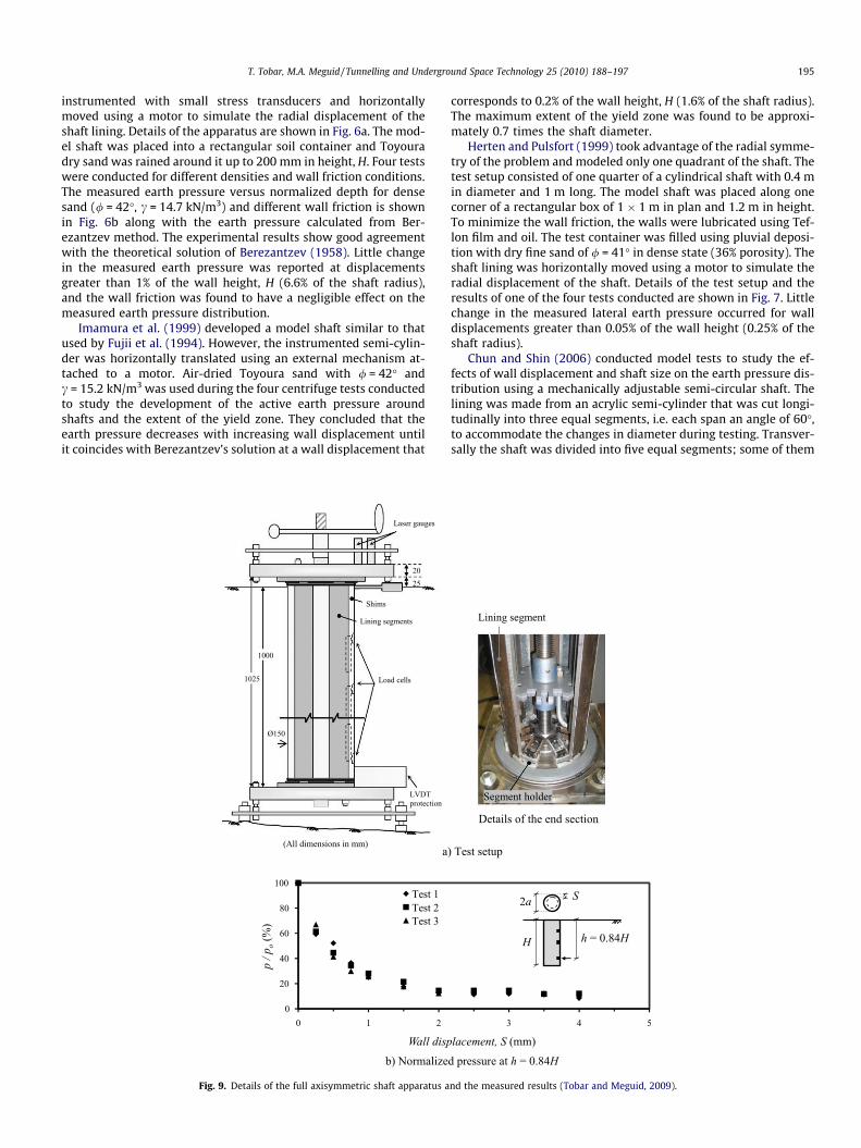
Tobar and Meguid (2009) conducted a series of tests under nor-mal gravity to investigate the changes in lateral earth pressure dueto radial displacement of the shaft lining. The developed apparatusallowed for the modeling of both the full geometry of the shaft andthe radial displacement of the lining. It was built using six curvedlining segments held vertically using segment holders (Fig. 9a). Asimple mechanism was developed to translate the lining segments

Table 1Comparison of the required wall displacements for active condition.

Prototype Model

SaSemi-cylinder (non-segmented)

Quarter-cylinder (non-segmented)

Semi-cylinder (segmented)

Full cylinder (segmented)

a Radial wall displacement.b Wall height.c Shaft radius.

radially; it consisted mainly of steel hinges that connected the seg-ment holders to central nuts. These nuts pass through a centralthreaded rod extended along the shaft axis. As the axial rod was ro-tated, the nuts moved vertically, pulling the segment holders radi-ally inwards and consequently the shaft lining was uniformlytranslated.

The model shaft (0.15 m in diameter and 1 m long) was placedinto a circular container of 1.22 m diameter and 1.07 m depth. Thecontainer was filled with coarse dry sand (/ = 41�; c = 14.7 kN/m3)using pluvial deposition. The axisymmetric active earth pressurefully developed when the wall displacements, S, ranged between0.2% and 0.3% of the wall height, H. It was concluded that forS P 0.1% H, the measured pressures fell into the range predictedby Cheng and Hu (2005); and that at S P 0.3% H, the measuredpressures closely followed the pressure distributions calculatedusing Terzaghi (1943) and Berezantzev (1958) methods.

3.4. Discussion of experimental investigations

Table 1 shows a summary of the required wall displacement forestablishing active conditions. To simplify the design and opera-tion of the shaft models, simplified mechanisms were used to re-duce the shaft diameter uniformly. It is evident that noagreement has been reached among researchers as to the requiredwall movement to reach active conditions. The displacement ran-ged from 0.05% to 1.8% of the shaft height as shown in Table 1. This

Required wall movement (S) to reach active condition Soil

� Fujii et al. (1994) Dense sandS P 1%Hb

orS P 6.6% ac

� Imamura et al. (1999)S = 0.2% HorS = 1.6% a

� Herten and Pulsfort (1999) Dense sandS = 0.05% HorS = 0.25% a

� Chun and Shin (2006) Dense sand0.6% H < S < 1.8% Hor0.15% a < S < 0.4% a

� Tobar and Meguid (2009) Loose sandS P 0.2% HorS P 2.5% a

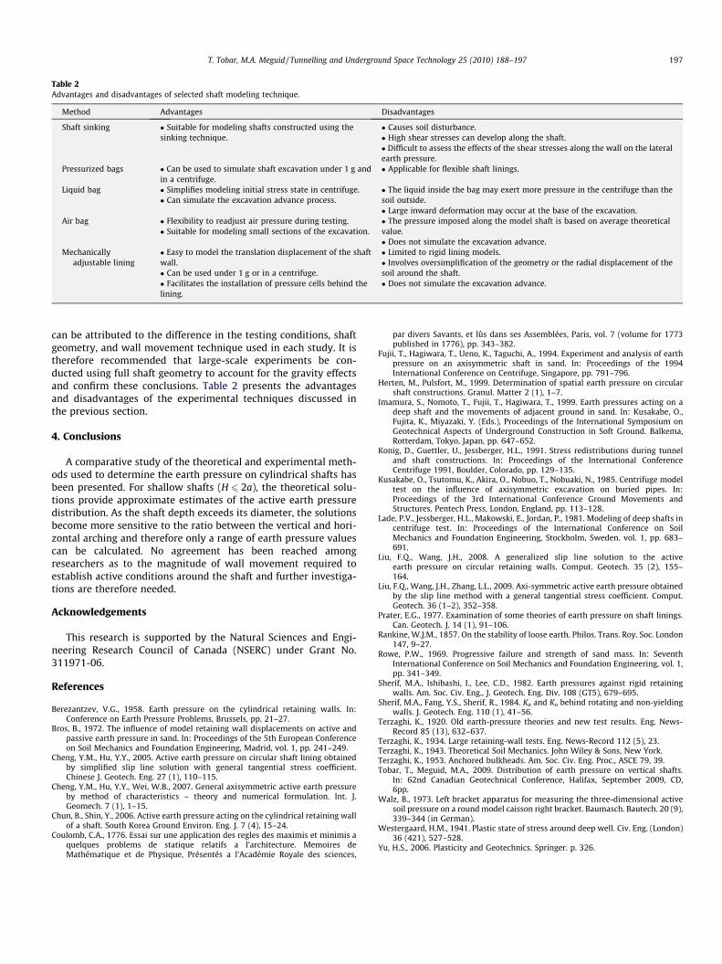
Table 2Advantages and disadvantages of selected shaft modeling technique.

Method Advantages Disadvantages

Shaft sinking � Suitable for modeling shafts constructed using thesinking technique.

� Causes soil disturbance.� High shear stresses can develop along the shaft.� Difficult to assess the effects of the shear stresses along the wall on the lateralearth pressure.

Pressurized bags � Can be used to simulate shaft excavation under 1 g andin a centrifuge.

� Applicable for flexible shaft linings.

Liquid bag � Simplifies modeling initial stress state in centrifuge. � The liquid inside the bag may exert more pressure in the centrifuge than thesoil outside.� Can simulate the excavation advance process.� Large inward deformation may occur at the base of the excavation.

Air bag � Flexibility to readjust air pressure during testing. � The pressure imposed along the model shaft is based on average theoreticalvalue.� Suitable for modeling small sections of the excavation.� Does not simulate the excavation advance.

Mechanicallyadjustable lining

� Easy to model the translation displacement of the shaftwall.

� Limited to rigid lining models.� Involves oversimplification of the geometry or the radial displacement of thesoil around the shaft.� Can be used under 1 g or in a centrifuge.� Does not simulate the excavation advance.� Facilitates the installation of pressure cells behind the

lining.


can be attributed to the difference in the testing conditions, shaftgeometry, and wall movement technique used in each study. It istherefore recommended that large-scale experiments be con-ducted using full shaft geometry to account for the gravity effectsand confirm these conclusions. Table 2 presents the advantagesand disadvantages of the experimental techniques discussed inthe previous section.

4. Conclusions

A comparative study of the theoretical and experimental meth-ods used to determine the earth pressure on cylindrical shafts hasbeen presented. For shallow shafts (H 6 2a), the theoretical solu-tions provide approximate estimates of the active earth pressuredistribution. As the shaft depth exceeds its diameter, the solutionsbecome more sensitive to the ratio between the vertical and hori-zontal arching and therefore only a range of earth pressure valuescan be calculated. No agreement has been reached amongresearchers as to the magnitude of wall movement required toestablish active conditions around the shaft and further investiga-tions are therefore needed.

Acknowledgements

This research is supported by the Natural Sciences and Engi-neering Research Council of Canada (NSERC) under Grant No.311971-06.

References

Berezantzev, V.G., 1958. Earth pressure on the cylindrical retaining walls. In:Conference on Earth Pressure Problems, Brussels, pp. 21–27.

Bros, B., 1972. The influence of model retaining wall displacements on active andpassive earth pressure in sand. In: Proceedings of the 5th European Conferenceon Soil Mechanics and Foundation Engineering, Madrid, vol. 1, pp. 241–249.

Cheng, Y.M., Hu, Y.Y., 2005. Active earth pressure on circular shaft lining obtainedby simplified slip line solution with general tangential stress coefficient.Chinese J. Geotech. Eng. 27 (1), 110–115.

Cheng, Y.M., Hu, Y.Y., Wei, W.B., 2007. General axisymmetric active earth pressureby method of characteristics – theory and numerical formulation. Int. J.Geomech. 7 (1), 1–15.

Chun, B., Shin, Y., 2006. Active earth pressure acting on the cylindrical retaining wallof a shaft. South Korea Ground Environ. Eng. J. 7 (4), 15–24.

Coulomb, C.A., 1776. Essai sur une application des regles des maximis et minimis aquelques problems de statique relatifs a l’architecture. Memoires deMathématique et de Physique, Présentés a l’Académie Royale des sciences,

par divers Savants, et lûs dans ses Assemblées, Paris, vol. 7 (volume for 1773published in 1776), pp. 343–382.

Fujii, T., Hagiwara, T., Ueno, K., Taguchi, A., 1994. Experiment and analysis of earthpressure on an axisymmetric shaft in sand. In: Proceedings of the 1994International Conference on Centrifuge, Singapore, pp. 791–796.

Herten, M., Pulsfort, M., 1999. Determination of spatial earth pressure on circularshaft constructions. Granul. Matter 2 (1), 1–7.

Imamura, S., Nomoto, T., Fujii, T., Hagiwara, T., 1999. Earth pressures acting on adeep shaft and the movements of adjacent ground in sand. In: Kusakabe, O.,Fujita, K., Miyazaki, Y. (Eds.), Proceedings of the International Symposium onGeotechnical Aspects of Underground Construction in Soft Ground. Balkema,Rotterdam, Tokyo, Japan, pp. 647–652.

Konig, D., Guettler, U., Jessberger, H.L., 1991. Stress redistributions during tunneland shaft constructions. In: Proceedings of the International ConferenceCentrifuge 1991, Boulder, Colorado, pp. 129–135.

Kusakabe, O., Tsutomu, K., Akira, O., Nobuo, T., Nobuaki, N., 1985. Centrifuge modeltest on the influence of axisymmetric excavation on buried pipes. In:Proceedings of the 3rd International Conference Ground Movements andStructures. Pentech Press, London, England, pp. 113–128.

Lade, P.V., Jessberger, H.L., Makowski, E., Jordan, P., 1981. Modeling of deep shafts incentrifuge test. In: Proceedings of the International Conference on SoilMechanics and Foundation Engineering, Stockholm, Sweden. vol. 1, pp. 683–691.

Liu, F.Q., Wang, J.H., 2008. A generalized slip line solution to the activeearth pressure on circular retaining walls. Comput. Geotech. 35 (2), 155–164.

Liu, F.Q., Wang, J.H., Zhang, L.L., 2009. Axi-symmetric active earth pressure obtainedby the slip line method with a general tangential stress coefficient. Comput.Geotech. 36 (1–2), 352–358.

Prater, E.G., 1977. Examination of some theories of earth pressure on shaft linings.Can. Geotech. J. 14 (1), 91–106.

Rankine, W.J.M., 1857. On the stability of loose earth. Philos. Trans. Roy. Soc. London147, 9–27.

Rowe, P.W., 1969. Progressive failure and strength of sand mass. In: SeventhInternational Conference on Soil Mechanics and Foundation Engineering, vol. 1,pp. 341–349.

Sherif, M.A., Ishibashi, I., Lee, C.D., 1982. Earth pressures against rigid retainingwalls. Am. Soc. Civ. Eng., J. Geotech. Eng. Div. 108 (GT5), 679–695.

Sherif, M.A., Fang, Y.S., Sherif, R., 1984. Ka and Ko behind rotating and non-yieldingwalls. J. Geotech. Eng. 110 (1), 41–56.

Terzaghi, K., 1920. Old earth-pressure theories and new test results. Eng. News-Record 85 (13), 632–637.

Terzaghi, K., 1934. Large retaining-wall tests. Eng. News-Record 112 (5), 23.Terzaghi, K., 1943. Theoretical Soil Mechanics. John Wiley & Sons, New York.Terzaghi, K., 1953. Anchored bulkheads. Am. Soc. Civ. Eng. Proc., ASCE 79, 39.Tobar, T., Meguid, M.A., 2009. Distribution of earth pressure on vertical shafts.

In: 62nd Canadian Geotechnical Conference, Halifax, September 2009, CD,6pp.

Walz, B., 1973. Left bracket apparatus for measuring the three-dimensional activesoil pressure on a round model caisson right bracket. Baumasch. Bautech. 20 (9),339–344 (in German).

Westergaard, H.M., 1941. Plastic state of stress around deep well. Civ. Eng. (London)36 (421), 527–528.

Yu, H.S., 2006. Plasticity and Geotechnics. Springer. p. 326.

tunnelling and underground space technology - geo...

Documents