evaluation of soil–pipe interaction under relative axial...
TRANSCRIPT

Evaluation of Soil–Pipe Interaction underRelative Axial Ground Movement
Masood Meidani1; Mohamed A. Meguid, Ph.D., P.Eng., M.ASCE2;and Luc E. Chouinard, Ph.D., P.Eng.3
Abstract: The expansion of urban communities around the world resulted in the installation of utility pipes near existing natural or artificialslopes. These pipes can experience significant increase in axial earth pressure as a result of possible slope movement in the pipeline direction.This research aims at utilizing the discrete-element method to investigate the response of a buried pipeline in granular material subjectedto axial soil movement. To determine the input parameters needed for the discrete-element analysis, calibration is performed using triaxial anddirect shear test data and the microscopic parameters are determined by matching the numerical and experimental results. The soil–pipesystem is then modeled and the detailed behavior of the pipe and the surrounding soil as well as their interaction at the particle-scale level arepresented. Conclusions are made regarding the suitability of the empirical approach used in practice to estimate the axial soil resistance indifferent soil conditions. This study suggests that caution should be exercised in calculating axial soil resistance to relative pipe movement indense sand material. A suitable lateral earth pressure coefficient should be determined in these cases as a function of the soil and pipeproperties. DOI: 10.1061/(ASCE)PS.1949-1204.0000269. © 2017 American Society of Civil Engineers.
Author keywords: Soil–structure interaction; Discrete-element method (DEM); Buried pipes; Axial movement.
Introduction
Buried pipes are considered to be among the most economical andsafe methods of transporting natural resources (e.g., oil, natural gas,and water distribution networks). Permanent ground deformationresulting from earthquakes or movement of nearby slopes can im-pose additional loads on the pipe leading to unacceptable deforma-tion and pipe separation from the surrounding soil. A report of theEuropean Gas Pipeline Incident Data Group (2005) has indicatedthat ground movement represents the fourth major cause of gaspipeline failure with close to half of the reported cases resulting inpipe rupture.
The response of buried pipes to slope movements depends onthe orientation of the pipeline with respect to the moving slope. Ifthe pipe axis is parallel to the direction of the sliding soil, the pipewould be subjected to longitudinal (axial) strains and the pipe ex-periences either tensile or compressive stresses. The second condi-tion occurs when the axis of the pipe is normal to the soil movementdirection and, in this case, the relative soil movement imposes lat-eral deformation to the pipe resulting in strains and stresses on thepipe wall due to the development of bending moments and shearforces. ASCE (1984) recommended a closed-form solution to
determine the axial loads on buried pipes in cohesionless soilsusing the following expression:
FA ¼ γ 0 ×H × ðπDLÞ ×�1þ K0
2
�× tanðδÞ ð1Þ
where FA = axial soil resistance; γ 0 = soil effective unit weight;H =depth from ground surface to the pipe springline; D = pipe outerdiameter; L = pipe length; K0 = coefficient of lateral earth pressureat rest; and δ = friction angle between the soil and the pipe.
Over the past few decades, researchers have studied soil–pipeinteraction using experimental, theoretical, and numerical methods(e.g., Newmark and Hall 1975; Trautmann and O’Rourke 1983;O’Rourke and Nordberg 1992; Honegger and Nyman 2002; Chanand Wong 2004; Karimian et al. 2006; Wijewickreme et al. 2009;Daiyan et al. 2011; Rahman and Taniyama 2015; Liu et al. 2015;Almahakeri et al. 2016; Zhang et al. 2016). Most of the numericalanalyses were performed using the finite-element (FE) method.Yimsiri et al. (2004) used FE analysis to study soil–pipe interactionunder lateral and upward soil movements in a deep burial condition.Guo and Stolle (2005) investigated the lateral earth pressure onburied pipes and concluded that capturing large soil movementinteracting with a buried conduit is challenging using continuumapproaches. Almahakeri et al. (2016) conducted a series of three-dimensional (3D) FE simulations to examine the longitudinal bend-ing in buried glass fiber–reinforced polymer (GFRP) pipes subjectedto lateral earth movements and compared the results with measureddata. Most recently, Zhang et al. (2016) studied the mechanicalbehavior of a buried steel pipeline crossing a landslide area usingfinite-element analysis and highlighted the role of soil and pipelineparameters on the behavior of the system. Although soil–structureinteraction with large deformation can bemodeled using a multiscaleapproach (Hughes 1995) or adaptive remeshing (Zienkiewicz andHuang 1990), modeling particle movement and unpredictable dis-continuities near existing pipes is very scarce in the literature.
The discrete-element method (DEM) has proven to be suitablefor modeling granular material and large deformation. The method
1Graduate Student, Dept. of Civil Engineering and Applied Mechanics,Univ. of McGill, 817 Sherbrooke St. W., Montreal, QC, Canada H3A 0C3.E-mail: [email protected]
2Associate Professor, Dept. of Civil Engineering and AppliedMechanics, Univ. of McGill, 817 Sherbrooke St. W., Montreal, QC, CanadaH2A 0C3 (corresponding author). ORCID: http://orcid.org/0000-0002-5559-194X. E-mail: [email protected]
3Associate Professor, Dept. of Civil Engineering and AppliedMechanics, Univ. of McGill, 817 Sherbrooke St. W., Montreal, QC, CanadaH2A 0C3. E-mail: [email protected]
Note. This manuscript was submitted on September 14, 2016; approvedon January 6, 2017; published online on March 25, 2017. Discussion periodopen until August 25, 2017; separate discussions must be submitted forindividual papers. This paper is part of the Journal of Pipeline SystemsEngineering and Practice, © ASCE, ISSN 1949-1190.
© ASCE 04017009-1 J. Pipeline Syst. Eng. Pract.
J. Pipeline Syst. Eng. Pract., -1--1
Dow
nloa
ded
from
asc
elib
rary
.org
by
McG
ill U
nive
rsity
on
03/2
5/17
. Cop
yrig
ht A
SCE
. For
per
sona
l use
onl
y; a
ll ri
ghts
res
erve
d.

was first proposed by Cundall and Strack (1979) and has been usedto analyze various geotechnical engineering problems. Laboratorytests have been successfully modeled by researchers using DEMto investigate the microscopic behavior of soil samples. Cui andO’Sullivan (2006) used discrete elements to study the macroscopicand microscopic behavior of granular soil under direct shear testconditions. Tran et al. (2013) proposed a finite–discrete elementframework for the 3D modeling of geogrid–soil interaction underpullout loading condition. Also, Tran et al. (2014) conducted three-dimensional discrete-element analysis to study the earth pressuredistribution on cylindrical shafts. The analysis allowed for the soilarching and radial pressure on the shaft wall to be visualized. Fur-thermore, Ahmed et al. (2015) conducted laboratory experimentsand finite–discrete element analysis to study the role of geogridreinforcement in reducing earth pressure on buried pipes. Ithas been shown in these studies that discrete-element or coupledfinite–discrete element approaches are effective in capturing theresponse of structural elements such as pipe and geogrid and theirinteraction with the surrounding soils.
This study presents the results of a three-dimensional discrete-element investigation that has been conducted to examine theresponse of a steel pipe buried in dense granular material and sub-ject to axial loading. A suitable discrete-element packing method isfirst utilized to prepare a soil sample with predefined properties.Material calibration is then performed using standard triaxialand direct shear tests to determine the input parameters neededfor the discrete-element simulation. The calculated response ofthe pipe is compared with the reported experimental results. Thevalidated model is used to determine the distribution of radial earthpressure on the pipe wall and understand the changes in in situ pres-sure around the pipe during and after the pullout process. The appli-cability of the available closed-form solution is also evaluated.
Discrete-Element Method
The DEM generally models the interaction between particles as adynamic process that reaches static equilibrium when the internaland external forces are balanced. Displacement and rotation of eachparticle are usually determined using Newton’s and Euler’s equa-tions. The discrete-element simulations reported in this study areperformed using the open source code YADE (Kozicki and Donzé2008; Šmilauer et al. 2010). Spherical particles of different sizes areadopted to represent the grain size distribution of the backfill soil.The contact law between particles is selected from the YADE li-brary. It includes Cundall’s linear elastic-plastic law with capabilityof transmitting moments between particles. The contact law isbriefly described as follows:
Following the collision of two particles A and B with radii rAand rB, contact penetration depth is defined as
Δ ¼ rA þ rB − d0 ð2Þ
where d0 = distance between the centers of particles A and B.Particle interaction is represented by the force vector F. This
vector can be decomposed into normal and tangential forces
FN ¼ KN · ΔN ; δFT ¼ −KT · δΔT ð3Þ
where FN = normal force; δFT = incremental tangential force;KN and KT = normal and tangential stiffnesses at the contact point;ΔN = normal penetration between the particles; and δΔT =incremental tangential displacement between the two particles.
The normal stiffness between particles A and B at the contactpoint is defined by
KN ¼ KAN · KB
N
KAN þ KB
Nð4Þ
where KAN and KB
N = particle normal stiffnessess calculated usingparticle radius r and material modulus E as follows:
KAN ¼ 2EArA and KB
N ¼ 2EBrB ð5Þ
Therefore, the normal stiffness at the contact point can bewritten as
KN ¼ 2EArA · 2EBrB2EArA þ 2EBrB
ð6Þ
The interaction tangential stiffness KT is defined as a ratio of thecomputed KN such that KT ¼ αKN .
The tangential force is limited by a threshold value expressed as
FT ¼ FT
kFTkkFNk · tanðϕmicroÞ if FT ≥ kFNk · tanðϕmicroÞ ð7Þ
where ϕmicro = microscopic friction angle between particles.The rolling resistance is determined using a rolling angular
vector θr obtained by summing the components of the incrementalrolling (Šmilauer et al. 2010)
θr ¼X
dθr ð8Þ
A resistant moment Mr is calculated by
Mr ¼ Kr · θr ð9Þwhere Kr = rolling stiffness of the interaction defined as
Kr ¼ βr ·
�rA þ rB
2
�2
· KT ð10Þ
The resistant moment is limited by a threshold value such that
Mr ¼θr
kθrk· ηr · kFNk ·
�rA þ rB
2
�
if Kr · θr ≥ ηr · kFNk ·
�rA þ rB
2
�ð11Þ
where ηr = dimensionless coefficient; and βr = rolling resistancecoefficient.
To ensure the stability of the DEM model, the critical time stepΔtcr is defined as
Δtcr ¼ miniffiffiffi2
p·
ffiffiffiffiffiffimi
Ki
rð12Þ
where mi = mass of particle i; and Ki = per-particle stiffness ofthe contacts in which particle i participates and min
iindictes the
minimum value.
Description of the Numerical Model
The experimental results used to validate the numerical modelare based on those reported by Wijewickreme et al. (2009). Theresponse of a buried steel pipe subjected to axial soil movementwas investigated in a test chamber (3.8 m long, 2.5 m wide, and1.82 m high) as depicted in Fig. 1. Graded Fraser River sand within situ density of 16 kN=m3 was used as a backfill soil. Themechanical characteristics of the sand have been also reportedbased on triaxial and direct shear tests conducted under confining
© ASCE 04017009-2 J. Pipeline Syst. Eng. Pract.
J. Pipeline Syst. Eng. Pract., -1--1
Dow
nloa
ded
from
asc
elib
rary
.org
by
McG
ill U
nive
rsity
on
03/2
5/17
. Cop
yrig
ht A
SCE
. For
per
sona
l use
onl
y; a
ll ri
ghts
res
erve
d.

pressures that range from 15 to 50 kPa. A summary of the mechani-cal characteristics of the backfill soil is given in Table 1. Thesteel pipe used in the experiments has an outside diameter of46 mm and a wall thickness of 13 mm. The interface friction angle(δ) between the backfill material and the steel pipe was reported tobe 36°. The pipe is placed over 0.7 m of bedding layer up tothe springlines and covered with 1.15 m of the backfill material.This corresponds to a height-to-diameter ratio (H=D) of 2.5.
The numerical model has been developed in this study such thatit replicates the geometry and test procedure used in the experi-ments. All components are generated inside the YADE package.Various packing algorithms can be used to generate DEM samplesfor both standard soil tests and large-scale pullout simulations.Techniques such as the compression method (Cundall and Strack1979), gravitational method (Ladd 1978), triangulation-based ap-proach (Labra and Onate 2009), and radius expansion method(PFC 2D) are widely used for this purpose.
Generating the Discrete-Element Particles
The soil sample is generated in this study using the radius expan-sion method following a grain size distribution similar to that of thebackfill material. Given the size of the physical model, it is numeri-cally impractical to simulate millions of particles with their actualsize. Therefore, particle upscaling with two different scale factorshas been adopted to gradually reduce the number of particles andmaintain the time step size at a reasonable value. In this process, abalance between the computional costs and the scaling effects onthe global response needs to be considered.The soil in the testchamber is divided into four zones as illustrated in Fig. 2. A particlescale factor of 90 is used in Zone 1, which represents the areaimmediately around the pipe, and increases to 140 in the remainingzones. A small scale factor is applied to particles in the close vicin-ity of the pipe to improve the contact between the soils and pipe.The selected scale factors are also supported by the findings of
previous researchers. Potyondy and Cundall (2004) noted that whenthe number of particles used in a discrete-element simulation is largeenough (more than 265,000 particles in this study using the men-tioned scale factors), the macroscopic response becomes indepen-dent of the particle size. Also, Tran et al. (2014) evaluated theeffect of different scale factors in analyzing soil–structure interactionand confirmed that when the number of particles is greater than245,000, the scale factor has an insignificant effect on the overallresponse of the system. Furthermore, Ahmed et al. (2015) suggestedthat creating a DEM sample with the number of soil particles around300,000 makes the global response of the system insensitive to thechange in particle size. The grain size distributions of the backfillmaterial and the particles in the different zones are shown in Fig. 3.
A cloud of noncontacting particles is first generated inside thebox for each zone following a predetermined particle size distribu-tion and scale factor. Particles located within the pipeline areaare then removed. The radius expansion method is applied to eachzone to achieve a target porosity of 0.41, which corresponds tothat of the experiment. The radius expansion method is known togenerate a specimen with an isotropic stress state (O’Sullivan2011). To dissipate this effect, each zone was subjected to gravityforces and allowed to reach equilibrium. The entire packing, in-cluding the four different zones, is then assembled under gravity
Pipe Pullout
1.82
m
Fig. 1. Configuration of the modeled experiments
Table 1. Mechanical Characteristics of Fraser River Sand
Parameter Value
Particle density (kg=m3) 2,720ϕpeak (degrees) 45ϕcv (degrees) 33ψ (degrees) 15Cohesion (kN=m2) 0Ei (MPa) 36ν 0.3γ ðkg=m3Þ for Dr ¼ 75% (dense sand) 1,600
Fig. 2. Schematic showing the different particle packing zones aroundthe pipe
0
10
20
30
40
50
60
70
80
90
100
0.01 0.1 1 10 100 1000
Perc
ent p
assi
ng (
%)
Grain diameter (mm)
Fraser River sand (Scale = 1)
DE in zone 1(Scale = 90)
DE in zones 2, 3 &4(Scale = 140)
Fig. 3. Grain size distribution with particle upscaling
© ASCE 04017009-3 J. Pipeline Syst. Eng. Pract.
J. Pipeline Syst. Eng. Pract., -1--1
Dow
nloa
ded
from
asc
elib
rary
.org
by
McG
ill U
nive
rsity
on
03/2
5/17
. Cop
yrig
ht A
SCE
. For
per
sona
l use
onl
y; a
ll ri
ghts
res
erve
d.
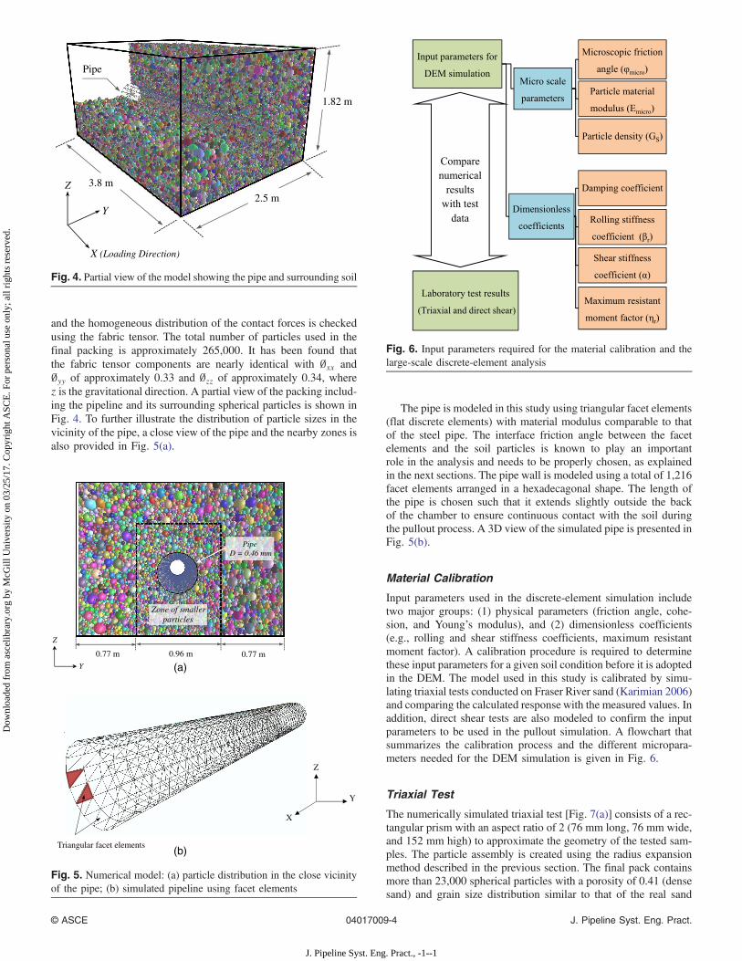
and the homogeneous distribution of the contact forces is checkedusing the fabric tensor. The total number of particles used in thefinal packing is approximately 265,000. It has been found thatthe fabric tensor components are nearly identical with ∅xx and∅yy of approximately 0.33 and ∅zz of approximately 0.34, wherez is the gravitational direction. A partial view of the packing includ-ing the pipeline and its surrounding spherical particles is shown inFig. 4. To further illustrate the distribution of particle sizes in thevicinity of the pipe, a close view of the pipe and the nearby zones isalso provided in Fig. 5(a).
The pipe is modeled in this study using triangular facet elements(flat discrete elements) with material modulus comparable to thatof the steel pipe. The interface friction angle between the facetelements and the soil particles is known to play an importantrole in the analysis and needs to be properly chosen, as explainedin the next sections. The pipe wall is modeled using a total of 1,216facet elements arranged in a hexadecagonal shape. The length ofthe pipe is chosen such that it extends slightly outside the backof the chamber to ensure continuous contact with the soil duringthe pullout process. A 3D view of the simulated pipe is presented inFig. 5(b).
Material Calibration
Input parameters used in the discrete-element simulation includetwo major groups: (1) physical parameters (friction angle, cohe-sion, and Young’s modulus), and (2) dimensionless coefficients(e.g., rolling and shear stiffness coefficients, maximum resistantmoment factor). A calibration procedure is required to determinethese input parameters for a given soil condition before it is adoptedin the DEM. The model used in this study is calibrated by simu-lating triaxial tests conducted on Fraser River sand (Karimian 2006)and comparing the calculated response with the measured values. Inaddition, direct shear tests are also modeled to confirm the inputparameters to be used in the pullout simulation. A flowchart thatsummarizes the calibration process and the different micropara-meters needed for the DEM simulation is given in Fig. 6.
Triaxial Test
The numerically simulated triaxial test [Fig. 7(a)] consists of a rec-tangular prism with an aspect ratio of 2 (76 mm long, 76 mm wide,and 152 mm high) to approximate the geometry of the tested sam-ples. The particle assembly is created using the radius expansionmethod described in the previous section. The final pack containsmore than 23,000 spherical particles with a porosity of 0.41 (densesand) and grain size distribution similar to that of the real sand
2.5 m
1.82 m
Pipe
3.8 m
X
Y
Z
(Loading Direction)
Fig. 4. Partial view of the model showing the pipe and surrounding soil
Pipe D = 0.46 mm
Zone of smaller particles
0.77 m Y
Z
0.96 m 0.77 m
Triangular facet elements
X
Y
Z
(a)
(b)
Fig. 5. Numerical model: (a) particle distribution in the close vicinityof the pipe; (b) simulated pipeline using facet elements
Fig. 6. Input parameters required for the material calibration and thelarge-scale discrete-element analysis
© ASCE 04017009-4 J. Pipeline Syst. Eng. Pract.
J. Pipeline Syst. Eng. Pract., -1--1
Dow
nloa
ded
from
asc
elib
rary
.org
by
McG
ill U
nive
rsity
on
03/2
5/17
. Cop
yrig
ht A
SCE
. For
per
sona
l use
onl
y; a
ll ri
ghts
res
erve
d.

material. The numerical simulation includes two stages: (1) thesample is compressed up to a target confining stress of 25, 35, or50 kPa; and (2) the top wall is allowed to move downward at aconstant strain rate to impose the deviatoric load while the stressesat the side walls are kept constant.
The interaction between particles is simulated using a contactmodel that considers traction, compression, bending, and twistingwith cohesion and friction based on Mohr-Coulomb failurecriterion. Plassiard et al. (2009) proposed a calibration procedurethat involves elastic parameters (E, KT=KN , βr) as well as ruptureparameters (ϕmicro and ηr). These parameters are determined tosatisfy the correct shape of the stress-strain curve and match theinitial Young’s modulus Ei, Poisson’s ratio ν, dilation angle ψ, andfriction angle ϕ of the material. The calibration is performed for aconfining pressure of 25 kPa and the obtained parameters are con-firmed by repeating the analysis for confining pressures of 35 and50 kPa. Fig. 7(b) presents the results of the discrete-element analy-sis along with the experimental data for all ranges of confiningpressures. The soil properties obtained from the triaxial test simu-lation for confining pressure of 25 kPa are summarized in Table 2.
Direct Shear Test
Modeling the direct shear test is used to confirm the macroscopicand microscopic parameters (Tables 2 and 3) to be used in the sim-ulation. The direct shear test (60 × 60 × 25 mm) was based on thatreported by Karimian (2006) for Fraser River sand under three dif-ferent normal stresses (20, 35, and 53 kPa). The discrete-elementpacking used in the direct shear test was created such that it hassimilar characteristics as that described in the triaxial test includingporosity, coordination number (Nc), and fabric tensor (Φij). Thesample porosity and coordination numbers at the initial state werefound to be 0.41 and 5.5, respectively. As shown in Fig. 8(a), aspecimen is created using the radius expansion method with a totalof 24,688 spheres and using a scale factor 5. The input parametersgiven in Table 3 are then assigned to the particles. The results of thedirect shear test for different normal stresses is shown in Fig. 8(b).The overall trend and the maximum shear stress values are found tobe consistent with the laboratory results. A slightly softer responseis observed for shear displacements of less than 0.5 mm. This maybe attributed to the difference in particle shapes as compared tothe spherical particles used in the discrete-element analysis. Similarobservation was made by Yan (2008).
Modeling the Pullout Procedure
Following the material calibration, a final specimen is created andthe properties are assigned to the discrete particles. No friction isused for the interaction between the particles and the walls of thebox, which is similar to the condition of the experiments to elimi-nate the boundary effects. A parametric study is conducted to ex-amine the effect of friction angle of the facets (used to model thepipe) on the pullout response. Results indicated that the soil–pipesystem is sensitive to the interface friction and a friction angle of30° was found to correspond to a maximum pullout force thatmatches the experimental data.
The pullout procedure is numerically simulated under dis-placement control with a movement rate of 50 mm=s applied tothe facets to be consistent with the experiment. The pipe wasincrementally pulled until a maximum displacement of 200 mmwas reached. The corresponding pullout force is captured duringthe simulation by summing the forces on the facets in the pullingdirection.
0
50
100
150
200
250
300
0 1 2 3 4 5 6 7
Axi
al S
tres
s, σ
1(k
Pa)
Axial strain, (%)
Experimental
DEM Simulation
σ3 = 50 kPa
σ3 = 35 kPa
σ3 = 25 kPa
76 mm
152 mm
76 mm
(a)
(b)
Fig. 7. Triaxial tests used for the material calibration: (a) tested sample;(b) results
Table 2. Soil Properties Based on Triaxial Tests with 25-kPa ConfiningStress
Parameter Value
ϕpeak (degrees) 45ψ (degrees) 15Ei (MPa) 34ν 0.28
Table 3. Selected Properties Used in Discrete-Element Analysis
Parameter Value
Particle density (kg=m3) 2,720Particle material modulus E (MPa) 150KT=KN ratio 0.7βr 0.15ϕmicro (degrees) 35ηr 1Damping ratio 0.2
© ASCE 04017009-5 J. Pipeline Syst. Eng. Pract.
J. Pipeline Syst. Eng. Pract., -1--1
Dow
nloa
ded
from
asc
elib
rary
.org
by
McG
ill U
nive
rsity
on
03/2
5/17
. Cop
yrig
ht A
SCE
. For
per
sona
l use
onl
y; a
ll ri
ghts
res
erve
d.

Radial Earth Pressure Distribution
After the final particle assembly in the chamber and the assignmentof input parameters, the pipe and the surrounding particles wereallowed to freely move under gravity. The initial stress distributionacting on the pipe is examined and compared with the analyticalsolution. The equation proposed by Hoeg (1968) allows for theradial pressure (σr) on buried pipes to be determined as follows:
σr ¼1
2P
�ð1þ kÞ
�1 − a1
�D2r
�2�
− ð1 − kÞ�1 − 3a2
�D2r
�4 − 4a3
�D2r
�2�cos 2θ
�ð13Þ
where D = pipe diameter; r = distance from the pipe center to thesoil element under analysis; k = lateral earth pressure coefficient atrest; P = soil vertical stress; θ = angle of inclination from the spring-line; and a1, a2, and a3 = constants.
A comparison of the initial radial pressures calculated usingDEM and that of Hoeg’s solution at selected locations is shownin Fig. 9. The pressure values are presented on opposite sides ofthe polar chart. The contact pressure ranged from 15 kPa at thecrown (angle 0°) to approximately 20 kPa at the invert (angle180°), which is consistent with the expected distribution for rigidpipes.
Vertical stress distribution in soil is also examined and com-pared with the expected values. To record macroscopic stress
components, a measurement box of volume V is used and the aver-age stress within the box is calculated as
σij ¼1
V
XNc
c¼1
xc;ifc;j ð14Þ
where Nc = number of contacts within the measurement box; fc;j =contact force vector at contact c; xc;i = branch vector connectingtwo contact particles A and B; and indexes i and j are the Cartesiancoordinates.
The soil chamber is divided into three regions [Fig. 10(a)] andthe vertical stresses are calculated in each region using Eq. (14).Region 1 is selected near the wall to evaluate the effect of the rigidboundaries on the results. Regions 2 and 3 are chosen at the samedistance in the opposite side of the pipe to assess the homogeneityof the generated particle packing. Vertical stresses are obtained us-ing measurement boxes with dimensions of 0.25 × 0.25 × 0.25 mand the results are presented in Fig. 10(b). It can be seen that ver-tical stress distribution in Region 1 near the boundary is consistentwith the expected values ðγ 0zÞ. This signifies that the effect of thewalls on the calculated vertical soil pressures is negligible. In ad-dition, by comparing the vertical stress distribution in Regions 2and 3, it is evident that the particle packing used in the simulationis homogenous.
Evaluating the Applicability of the Closed-FormSolution
The relationship between the pullout force and corresponding pipedisplacement is shown in Fig. 11. To facilitate comparison betweenthe numerical and experimental results, the axial resistance FA isnormalized with respect to soil density (γ 0), pipe length (L), depth(H), and diameter (D) as represented by Eq. (15)
σn= 20 kPa
σn= 35 kPa
σn= 53 kPa
0
10
20
30
40
50
60
0 0.5 1 1.5 2
Shea
rst
ress
,τ(k
Pa)
Shear displacement (mm)
ExperimentDEM Simulation
Shearing direction
27 mm
60 mm
60 mm
(a)
(b)
Fig. 8.Direct shear tests used to confirm the input parameters: (a) testedsample; (b) results
0
5
10
15
20
25
30
Analytical solution
Numerical analysis
Fig. 9. Initial earth pressure distribution on the pipe (kPa)
© ASCE 04017009-6 J. Pipeline Syst. Eng. Pract.
J. Pipeline Syst. Eng. Pract., -1--1
Dow
nloa
ded
from
asc
elib
rary
.org
by
McG
ill U
nive
rsity
on
03/2
5/17
. Cop
yrig
ht A
SCE
. For
per
sona
l use
onl
y; a
ll ri
ghts
res
erve
d.
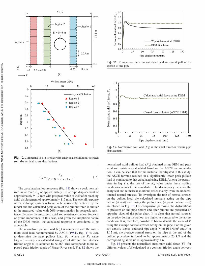
F 0A ¼ FA
γ 0 ×H × π ×D × Lð15Þ
The calculated pullout response (Fig. 11) shows a peak normal-ized axial force F 0
A of approximately 1.0 at pipe displacement ofapproximately 9–12 mm with postpeak value of 0.89 after reachingaxial displacement of approximately 115 mm. The overall responseof the soil–pipe system is found to be reasonably captured by themodel and the calculated peak value of the pullout force is similarto the measured value with 20% overestimation in postpeak resis-tance. Because the maximum axial soil resistance (pullout force) isof prime importance in this case, and given the simplified natureof the DEM model, the calculated response is considered to beacceptable.
The normalized pullout load (F 0A) is compared with the maxi-
mum axial load recommended by ASCE (1984). Eq. (1) is usedto determine the peak pullout load, FA. where the K0 value(K0 ¼ 1 − sinϕ 0) is calculated using ϕ 0 of 44° and the interfacefriction angle (δ) is assumed to be 36°. This corresponds to the re-ported peak friction angle of Fraser River sand. Fig. 12 shows the
normalized axial pullout load (F 0A) obtained using DEM and peak
axial soil resistance calculated based on the ASCE recommenda-tion. It can be seen that for the material investigated in this study,the ASCE formula resulted in a significantly lower peak pulloutload as compared to that calculated using DEM. Among the param-eters in Eq. (1), the use of the K0 value under these loadingconditions seems to be unrealistic. The discrepancy between theanalytical and numerical solutions arises mainly from the underes-timated normal stresses. To investigate the role of normal stresseson the pullout load, the calculated pressure acting on the pipebefore (at rest) and during the pullout test (at peak pullout load)are plotted in Fig. 13. For comparison purposes, the distributionsof pressure on the pipe before and after pullout are presented onopposite sides of the polar chart. It is clear that normal stresseson the pipe during the pullout are higher as compared to the at-restcondition. It is, therefore, possible to back-calculate the value of Kusing the average normal stresses acting on the pipe. For the givensoil density (dense sand) and pipe depth (γ 0 of 16 kN=m3 and H of1.12 m), the average normal stress on the pipe at the end of thepullout procedure is found to be approximately 23 kN and thecorresponding K value is approximately 1.6.
Fig. 14 presents the normalized maximum axial force (F 0A) for
different values of K calculated at a constant friction angle between
0
0.2
0.4
0.6
0.8
1
1.2
1.4
1.6
1.8
0 10 20 30 40
Dep
th (
m)
Vertical stress (kPa)
Analytical Solution
Region 1
Region 2
Region 3
2.5 m
D = 0.46 m
Region 3 Region 2
Region 1
0.25 m
0.1 0.25 0.6 m3 x 0.25 m
Y
Z
1.82
m
(a)
(b)
Fig. 10.Comparing in situ stresses with analytical solution: (a) selectedsoil; (b) vertical stress distributions
0.0
0.2
0.4
0.6
0.8
1.0
1.2
1.4
0 25 50 75 100 125 150
Nor
mal
ized
axi
al s
oil f
orce
, F' A
Pipe displacement (mm)
Wijewickreme et al. (2009)
DEM Simulation
Fig. 11. Comparison between calculated and measured pullout re-sponse of the pipe
0
0.2
0.4
0.6
0.8
1
1.2
1.4
0 25 50 75 100 125 150
Nor
mal
ized
axi
al s
oil f
orce
, F' A
Pipe displacement (mm)
Closed form solution (ASCE, 1984)
Calculated axial force using DEM
Fig. 12. Normalized soil load (F 0A) in the axial direction versus pipe
displacement
© ASCE 04017009-7 J. Pipeline Syst. Eng. Pract.
J. Pipeline Syst. Eng. Pract., -1--1
Dow
nloa
ded
from
asc
elib
rary
.org
by
McG
ill U
nive
rsity
on
03/2
5/17
. Cop
yrig
ht A
SCE
. For
per
sona
l use
onl
y; a
ll ri
ghts
res
erve
d.

the pipe and the backfill material (δ ¼ 36°). A lateral earth pressurecoefficient K of 1.8 was found to correspond to a reasonable agree-ment between the maximum axial soil resistance from the DEMresults and that calculated using Eq. (1). The back-calculated valueof K based on the average normal stress on the pipe during pulloutis found to be equal to 1.6.
It is evident from Fig. 14 that using Ko to represent the earthpressure on the pipe under pullout loading condition is not suitable,particularly for dense sand. The suggested value by ASCE (1984)for predicting the maximum axial soil resistance may be more suit-able for loose to medium backfill material. This can be attributed tothe dilation of dense sand that develops in the close vicinity of thepipe under large displacement resulting in a stress state that exceedsthe at-rest condition.
Soil Response to Pipe Movement
To illustrate the changes that develop in the backfill material aroundthe pipe as a result of the relative movement, the contact force net-work before and after the pullout test in both the transverse andlongitudinal directions are shown in Figs. 15 and 16, respectively.Each contact force is illustrated by a line connecting the centers oftwo contacting elements, while the width of the line is proportionalto the magnitude of the normal contact force. Fig. 15(a) shows thatthe density of the contact forces is homogeneous around the pipebefore applying the pullout load. As the pipe is pulled [Fig. 15(b)],soil particles start to move, resulting in volume change and anincrease in normal stresses acting on the pipe. This behavior ismanifested in the large contact forces observed in the vicinity ofthe pipe.
The pullout effect can be further examined by inspecting thecontact force distribution within the soil zones that are most af-fected by the pullout process. Zone A in Fig. 15(b) representsthe extent of the disturbed area around the pipe selected by com-paring the density of the contact forces around the pipe before andafter the pullout process. The shape of this zone resembles a circlewith radius of approximately 1.5 times the pipe diameter (1.5D).Contact forces are found to be denser and oriented radially withinthis zone.
Fig. 16 presents the variation in contact forces in the longitudi-nal direction looking downward at the soil surface. The results arepresented for the initial condition [Fig. 16(a)] and after pullout[Fig. 16(b)]. As the pipe is pulled out, the density of contact forcesincreased along the pipe (Zone B) with further increase in density
0
5
10
15
20
25
30
Analytical solution
Numerical analysis
Fig. 13. Normal stress distribution on the pipe before and after thepullout test (kPa)
0
0.2
0.4
0.6
0.8
1
1.2
1.4
1.6
1.8
0 25 50 75 100 125 150
Nor
mal
ized
axi
al s
oil f
orce
, FA
Pipe displacement (mm)
DEM Simulation
Ko=0.42
K=0.6
K=1
K=1.4
K=1.8
Kp=3.7
ASCE
at-rest coefficient (Ko)
passive coefficient (Kp)
Fig. 14. Normalized axial soil resistance using ASCE (1984) equationfor different K values
Y
Z
(a)
(b)
Fig. 15. Contact force network: (a) before pullout; (b) after pullout
© ASCE 04017009-8 J. Pipeline Syst. Eng. Pract.
J. Pipeline Syst. Eng. Pract., -1--1
Dow
nloa
ded
from
asc
elib
rary
.org
by
McG
ill U
nive
rsity
on
03/2
5/17
. Cop
yrig
ht A
SCE
. For
per
sona
l use
onl
y; a
ll ri
ghts
res
erve
d.
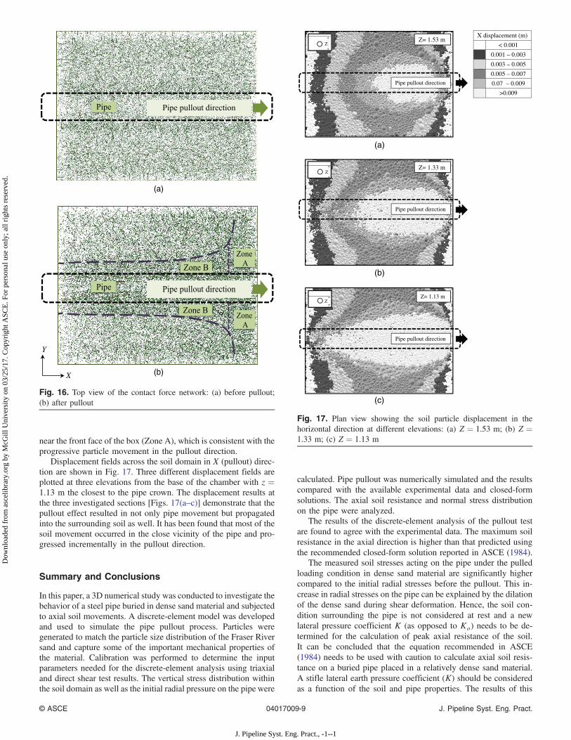
near the front face of the box (Zone A), which is consistent with theprogressive particle movement in the pullout direction.
Displacement fields across the soil domain in X (pullout) direc-tion are shown in Fig. 17. Three different displacement fields areplotted at three elevations from the base of the chamber with z ¼1.13 m the closest to the pipe crown. The displacement results atthe three investigated sections [Figs. 17(a–c)] demonstrate that thepullout effect resulted in not only pipe movement but propagatedinto the surrounding soil as well. It has been found that most of thesoil movement occurred in the close vicinity of the pipe and pro-gressed incrementally in the pullout direction.
Summary and Conclusions
In this paper, a 3D numerical study was conducted to investigate thebehavior of a steel pipe buried in dense sand material and subjectedto axial soil movements. A discrete-element model was developedand used to simulate the pipe pullout process. Particles weregenerated to match the particle size distribution of the Fraser Riversand and capture some of the important mechanical properties ofthe material. Calibration was performed to determine the inputparameters needed for the discrete-element analysis using triaxialand direct shear test results. The vertical stress distribution withinthe soil domain as well as the initial radial pressure on the pipe were
calculated. Pipe pullout was numerically simulated and the resultscompared with the available experimental data and closed-formsolutions. The axial soil resistance and normal stress distributionon the pipe were analyzed.
The results of the discrete-element analysis of the pullout testare found to agree with the experimental data. The maximum soilresistance in the axial direction is higher than that predicted usingthe recommended closed-form solution reported in ASCE (1984).
The measured soil stresses acting on the pipe under the pulledloading condition in dense sand material are significantly highercompared to the initial radial stresses before the pullout. This in-crease in radial stresses on the pipe can be explained by the dilationof the dense sand during shear deformation. Hence, the soil con-dition surrounding the pipe is not considered at rest and a newlateral pressure coefficient K (as opposed to Ko) needs to be de-termined for the calculation of peak axial resistance of the soil.It can be concluded that the equation recommended in ASCE(1984) needs to be used with caution to calculate axial soil resis-tance on a buried pipe placed in a relatively dense sand material.A stifle lateral earth pressure coefficient (K) should be consideredas a function of the soil and pipe properties. The results of this
X
Y
(a)
(b)
Fig. 16. Top view of the contact force network: (a) before pullout;(b) after pullout
X displacement (m)
< 0.001
0.001 – 0.003
0.003 – 0.005
0.005 – 0.007
0.07 – 0.009
>0.009
Z= 1.53 m
Z= 1.33 m
Z= 1.13 m
Pipe pullout direction
Z
Z
Pipe pullout direction
Z
Pipe pullout direction
(a)
(b)
(c)
Fig. 17. Plan view showing the soil particle displacement in thehorizontal direction at different elevations: (a) Z ¼ 1.53 m; (b) Z ¼1.33 m; (c) Z ¼ 1.13 m
© ASCE 04017009-9 J. Pipeline Syst. Eng. Pract.
J. Pipeline Syst. Eng. Pract., -1--1
Dow
nloa
ded
from
asc
elib
rary
.org
by
McG
ill U
nive
rsity
on
03/2
5/17
. Cop
yrig
ht A
SCE
. For
per
sona
l use
onl
y; a
ll ri
ghts
res
erve
d.
investigation suggest that a range of values between Ko and 2 isconsidered to be reasonable for pipelines under similar conditions.The numerical modeling approach proposed in this study hasproven to be efficient in modeling pipelines subjected to relativesoil movement and could be adapted for similar applications.
Acknowledgments
This research is supported by the Natural Sciences and EngineeringResearch Council of Canada (NSERC). Financial support providedby McGill Engineering Doctoral Award (MEDA) to the first authoris appreciated.
References
Ahmed, M. R., Tran, V. D. H., and Meguid, M. A. (2015). “On the roleof geogrid reinforcement in reducing earth pressure on buried pipes:Experimental and numerical investigations.” Soils Found., 55(3),588–599.
Almahakeri, M., Moore, I. D., and Fam, A. (2016). “Numerical study oflongitudinal bending in buried GFRP pipes subjected to lateral earthmovements.” J. Pipeline Syst. Eng. Pract., 10.1061/(ASCE)PS.1949-1204.0000237, 04016012.
ASCE. (1984). “Guidelines for the seismic design of oil and gas pipelinesystems, committee on gas and liquid fuel lifelines.” New York.
Chan, P. D. S., and Wong, R. C. K. (2004). “Performance evaluation ofa buried steel pipe in a moving slope: A case study.” Can. Geotech. J.,41(5), 894–907.
Cui, L, and O’Sullivan, C. (2006). “Exploring the macro-and micro-scaleresponse of an idealized granular material in the direct shear apparatus.”Geotechnique, 56(7), 455–468.
Cundall, P. A., and Strack, O. D. (1979). “A discrete numerical model forgranular assemblies.” Geotechnique, 29(1), 47–65.
Daiyan, N., Kenny, S., Phillips, R., and Popescu, R. (2011). “Investigatingpipeline-soil interaction under axial-lateral relative movements in thesand.” Can. Geotech. J., 48(11), 1683–1695.
European Gas Pipeline Incident Data Group. (2005). “6th EGIG Report1970–2004.” Rep. No. EGIG 05-R-0002, Groningen, Netherlands.
Guo, P. J., and Stolle, D. F. E. (2005). “Lateral pipe-soil interaction in sandwith reference to scale effect.” J. Geotech. Geoenviron. Eng., 10.1061/(ASCE)1090-0241(2005)131:3(338), 338–349.
Hoeg, K. (1968). “Stresses against underground structural cylinders.”J. Soil Mech. Found., 94(4), 833–858.
Honegger, D. G., and Nyman, D. J. (2002). “Guidelines for the seismicdesign and assessment of natural gas and liquid hydrocarbon pipelines.”Pipeline Research Council International, Arlington, VA.
Hughes, T. J. R. (1995). “Multiscale phenomena: Green’s functions, theDirichlet-to-Neumann formulation, subgrid scale models, bubblesand the origins of stabilized methods.” Comput. Methods Appl. Mech.Eng., 127(1), 387–401.
Karimian, H. (2006). “Response of buried steel pipelines subjected to lon-gitudinal and transverse ground movement.” Ph.D. thesis, Dept. of CivilEngineering, Univ. of British Columbia, Vancouver, BC, Canada.
Karimian, H., Wijewickreme, D., and Honegger, D. (2006). “Buriedpipelines subjected to transverse ground movement: Comparisonbetween full-scale testing and numerical modeling.” Proc., 25th Int.Conf. on Offshore Mechanics and Arctic Engineering, ASME,New York, 73–79.
Kozicki, J., and Donzé, V. F. (2008). “A new open-source software devel-oped for numerical simulations using discrete modeling methods.”Comput. Methods Appl. Mech. Eng., 197(49-50), 4429–4443.
Labra, C., and Onate, E. (2009). “High density sphere packing for discreteelement method simulations.” Commun. Numer. Methods Eng., 25(7),837–849.
Ladd, R. S. (1978). “Preparing test specimens using undercompaction.”Geotech. Test. J., 1(1), 16–23.
Liu, R., Guo, S., and Yan, S. (2015). “Study on the lateral soil resistanceacting on the buried pipeline.” J. Coastal Res., 73, 391–398.
Newmark, M., and Hall, W. J. (1975). “Pipeline design to resist large faultdisplacement.” Proc., U.S. National Conf. on Earthquake Engineering,Earthquake Engineering Research Institute, Oakland, CA, 416–425.
O’Rourke, M. J., and Nordberg, C. (1992). “Longitudinal permanentground deformation effects on buried continuous pipelines.” TechnicalRep. NCEER-92-0014, National Center for Earthquake EngineeringResearch, Buffalo, NY.
O’Sullivan, C. (2011). Particulate discrete element modeling, a geome-chanics perspective, Spon Press, New York.
PFC 2D version 3 [Computer software]. Itasca Consulting Group,Minneapolis.
Plassiard, J.-P., Belheine, N., and DonzâE, F.-V. (2009). “A spherical dis-crete element model: Calibration procedure and incremental response.”Granular Matter, 11(5), 293–306.
Potyondy, D. O., and Cundall, P. A. (2004). “A bonded-particle model forrock.” Int. J. Rock Mech. Min. Sci., 41(8), 1329–1364.
Rahman, M. A., and Taniyama, H. (2015). “Analysis of a buried pipelinesubjected to fault displacement: A DEM and FEM study.” Soil Dyn.Earthquake Eng., 71, 49–62.
Šmilauer, V., et al. (2010). “The Yade project.” ⟨http://yadedem.org/doc/⟩(Oct. 28, 2013).
Tran, V. D. H., Meguid, M. A., and Chouinard, L. E. (2013). “A finite-discrete element framework for the 3D modeling of geogrid-soil inter-action under pullout loading conditions.” Geotext. Geomembr., 37(1),1–9.
Tran, V. D. H., Meguid, M. A., and Chouinard, L. E. (2014). “Discreteelement and experimental investigations of the earth pressure distribu-tion on cylindrical shafts.” Int. J. Geomech., 10.1061/(ASCE)GM.1943-5622.0000277, 80–91.
Trautmann, C. H., and O’Rourke, T. D. (1983). “Behavior of pipe withdry sand under lateral and uplift loading.” Geotechnical EngineeringRep. 83-7, Cornell Univ., Ithaca, NY.
Wijewickreme, D., Karimian, H., and Honegger, D. (2009). “Responseof buried steel pipelines subjected to relative axial soil movement.”Can. Geotech. J., 46(7), 735–752.
Yan, W. M. (2008). “Effects of particle shape and microstructure onstrength and dilatancy during a numerical direct shear test.” Proc.,12th Int. Association for Computer Methods and Advances in Geome-chanics, India, 1340–1345.
Yimsiri, S., Soga, K., Yoshizaki, K., Dasari, G. R., and O’Rourke, T. D.(2004). “Lateral and upward soil-pipeline interactions in sand fordeep embedment conditions.” J. Geotech. Geoenviron. Eng., 10.1061/(ASCE)1090-0241(2004)130:8(830), 830–842.
Zhang, J., Liang, Z., and Han, C. (2016). “Mechanical behavior analysis ofthe buried steel pipeline crossing landslide area.” J. Pressure VesselTechnol., 138(5), 051702.
Zienkiewicz, O. C., and Huang, G. C. (1990). “A note on localization phe-nomena and adaptive finite-element analysis in forming processes.”Commun. Appl. Numer. Methods, 6(2), 71–76.
© ASCE 04017009-10 J. Pipeline Syst. Eng. Pract.
J. Pipeline Syst. Eng. Pract., -1--1
Dow
nloa
ded
from
asc
elib
rary
.org
by
McG
ill U
nive
rsity
on
03/2
5/17
. Cop
yrig
ht A
SCE
. For
per
sona
l use
onl
y; a
ll ri
ghts
res
erve
d.