transport phenomena in porous media ii || modeling turbulence in porous media

8 MODELING TURBULENCE IN POROUS MEDIA

J. L. LAGE*, M. J. S. DE LEMOS+ and D. A. NIELD^

* Department of Mechanical Engineering, Southern Methodist University, Dallas, TX

75275-0337, USA

email: j l l @ e n g r . s m u . e d u

^Departamento de Energia, Instituto Tecnologico de Aeronautica, 12228-900 Sao Jose

dos Campos, SP, Brazil

email: de l emos@mec . i t a . b r

^Department of Engineering Science, University of Auckland, Private Bag 92019, Auckland, New Zealand

email: d . n i e l d ( 9 a u c k l a n d . a c . n z

Abstract

Four available methodologies for developing macroscopic turbulence models for incompressible single-phase flow in rigid, fully saturated porous media are reviewed. The first method, known as the Antohe-Lage (A-L) method, starts with the closed volume-averaged equations, which are then averaged in time to produce the turbulence equations. The second, known as the Nakayama-Kuwahara (N-K) method, makes use, first, of the closed time-averaged equations, and then proceeds with volume-averaging for deriving the turbulence equations. These two methodologies lead, in general, to distinct sets of turbulence equations because of the dijRTerent averaging order, i.e., space-time and time-space, respectively. A third, and probably the most consistent method, based on double-decomposition, is the Pedras-de Lemos (P-dL) method. In this method, the momentum equation is closed by using the Hazen-Dupuit-Darcy model for the total drag effect only after the space-time averaging (or time-space averaging) is performed. Although for the P-dL method the averaging order is immaterial when deriving the turbulence momentum equation, the difference between space-time and time-space averaging remains in the k-e equations. Unfortunately, detailed experimental model validation, which remains to be seen, is tremendously challenging because of the need to obtain time-averaged and volume-averaged quantities simultaneously in order to compare experimental and analytical (numerical) results direcdy. A fourth method, the Travkin-Catton (T-C) morphology method, is discussed only briefly because it follows the N-K method (time-space integrating order) and no closure to the final equations is yet available.

Keywords: turbulence, modeling, transport, porous media, averaging

198

J.L.LAGEETAL. 199

8.1 INTRODUCTION

Modeling turbulent transport in porous media can impact several critical and practical engineering areas. For instance, the accurate simulation of turbulent air flow permeating through forests, where the vegetation is seen as a porous structure, is extremely important for predicting bio-diversity (spreading of seeds) and mitigation of fire propagation. The transport and dispersion of smog through heavily built cities can also benefit from the accurate modeling of turbulent flow through porous media.

Efficient and realistic overall pressure-drop along oil extraction porous wells is also very important. In this application, the flow of oil and gas along a radial-inward path is accelerated by getting near a more permeable region (the well) becoming turbulent. Proper mathematical characterization of the flow is necessary in order to reduce uncertainties on the well lifetime performance.

Processes of solidification and fusion of certain alloys are characterized by the presence of three distinct domains, namely, a fluid, a mushy and a solid zone. When the flow in the fluid zone is turbulent, the accurate prediction of the final product (the metal) depends on the proper characterization of the turbulent transport process inside the mushy zone. A similar process is the manufacturing of optical fiber and glass, which involves the turbulent flow of a doping gas during the melting process.

These engineering and environmental processes are only a few examples establishing the variety and importance of applications that can benefit from a proper mathematical analysis of turbulent flow in porous media. In a broader sense, the study of turbulence in porous media embraces fluid and thermal sciences, materials, chemical, geothermal, bio, petroleum and combustion engineering.

So far, the term turbulence has been used here to denote turbulence anywhere within the pores of the porous medium. The turbulent transport within the pore network of a porous medium can be studied, in principle, through direct numerical simulation. However, the direct numerical simulation at the pore (microscopic) level is impractical not only because of the tremendous computational effort required to resolve all the different turbulence scales, but also because of the additional effort required to access, map and resolve the complicated internal morphology of the porous medium.

Modeling is a natural alternative to direct numerical simulation. The objective of good modeling is to reduce the complexity of the mathematical formulation for studying the phenomenon. Averaging is a powerful modeling tool, which must be used carefully not to compromise the fundamental mathematical information ruling the phenomenon. When studying turbulent flow in individual fluid conduits, for instance, the Navier-Stokes equation can be time-averaged and closed with the stress-strain relations for the Reynolds stress, leading to the well-known k-e turbulence model. This model reduces the complexity of the problem by eliminating the need to follow the rapid fluctuations in time of fluid velocity and pressure, so characteristic of turbulence. Instead, the final model equation deals only with time-averaged quantities. Although information is invariably lost when time averaging the equations, it is hoped that the major characteristics of the transport process be retained by the model.

200 MODELING TURBULENCE IN POROUS MEDU

When considering transport in porous media, the complexity is the internal morphology of the porous medium, which is extremely complicated in general. In this case, volume averaging is the tool of choice. For instance, by volume averaging the Navier-Stokes equation, and closing the resulting equation with the Hazen-Dupuit-Darcy (HDD) model (also known as the Forchheimer-Darcy model), the macroscopic general momentum equation is obtained. This equation involves only volume-averaged quantities eliminating (as hoped!) the requirement for detailing the interior morphology of the porous medium. Again, information is invariably lost by the averaging process. Nevertheless, the major characteristics of the transport process are to be captured by the model.

To consider turbulence in porous media is to bring together the difficulties in modeling turbulence (time variation) and in modeling transport in porous media (space variation). A natural modeling approach is to simply apply the time averaging (for handling turbulence) and the space averaging (for handling the morphology) to the microscopic equations (valid at the pore level, e.g., Navier-Stokes). It is exactly at this point that modeling turbulence in porous media becomes excitingly challenging. For example, is the averaging order (time-space or space-time) important? If it is, then what is the proper order?

The main objective of this chapter is to attempt to answer these questions by reviewing and critiquing four different available methodologies for developing macroscopic turbulence models for incompressible single-phase flow in rigid, fully saturated porous media. These methods are the Antohe-Lage (A-L) space-time method, the Nakayama-Kuwahara (N-K) time-space method, the Pedras-de Lemos (P-dL) double-decomposition method, and the Travkin-Catton (T-C) morphology method. Although much is yet to be accomplished in this area, it is expected that the contribution herein will provide insight into the continuous progress in modeling turbulence in porous media.

8.2 TRANSITION TO TURBULENCE IN POROUS MEDIA

The topic of transition to turbulence in porous media is among the interesting topics reviewed by Lage (1998), who discussed several experimental studies related to transition to turbulence in porous media, and Masuoka (1999). It is important to point out that the available quantitative measurements indicating transition to turbulence are all local, i.e., performed at a particular location within a pore. We refer to these as pore-level or microscopic measurements.

The determination in a porous medium experiment of the critical Reynolds number at which turbulence appears is not a straightforward matter. Even considering a porous medium with simple internal morphology, say of conduit type in which the pore space consists essentially of tubes of varying cross-section. Here there is the possibility of relaminarization in the diverging portions of the tubes of turbulence that appears in converging portions. Ideally, one would like to put probes in the narrowest part of the tubes, but of course that is difficult in practice and almost certainly has not been achieved in experiments reported to date. Also, it should be noted that the appearance of a signal chaotic in time at a single position is probably an excellent indication, but not conclusive

J.L.LAGEETAL. 201

evidence, of the onset of turbulence. One needs to observe also what is happening at a neighboring point in order to be sure that turbulence is occurring.

This argument is because, for a constant volume flux through a tube, the mean velocity is inversely proportional to tube cross-section, and hence inversely proportional to the square of the tube diameter. The local Reynolds number, which involves the product of the mean velocity and the tube diameter, is thus inversely proportional to the tube diameter. This means, in the wider portions of the tube, that the local Re value may drop below the critical value necessary to maintain the turbulent state. In other words, relaminarization may occur. Using the same argument, the onset of turbulence is likely to occur first in those parts of the channel where the local Re is highest, namely in the narrowest part of the tubes. When porous media with more complicated internal morphology are considered, then the phenomenon of flow separation might come into play, inducing turbulence locally. The difficulty is not only to place a probe and measure the internal turbulence level but also to determine the location(s) within the pore network more prone to turbulence. For that, one would need to know the internal flow structure before performing the measurement.

Although controversial, see Lage and Antohe (2000), the pore-based Reynolds number Rep is commonly used in the literature for recognizing distinct flow regimes in porous media. Dybbs and Edwards (1984), for instance, used their pore-level experimental observations to classify the flow regimes as follows:

(a) Darcy, or viscous-drag, dominated flow regime (Rep < 1),

(b) Forchheimer, or form-drag, dominated flow regime (1 ~ 10 < Rep < 150),

(c) post-Forchheimer flow regime (unsteady laminar flow, 150 < Rep < 300), and

(d) fully turbulent flow (Rep > 300).

Keep in mind that the characterization of regimes (c) and (d) are based on point measurements (with probes placed at a specific location inside the porous medium). For Rep < 150, classical mathematical treatment of flow in porous media, see Lage (1998), invokes the notion of a representative elementary volume (REV), for which macroscopic, volume-averaged transport equations are derived and closed using empirical models, e.g., the HDD model. These macroscopic equations carry less detail of the flow pattern inside the REV, revealing only volume-averaged flow characteristics.

The mathematical description of the last regime, for high Reynolds number (Rep > 300), has given rise to interesting discussions in the literature and remains a controversial issue. Turbulence models presented in the literature for studying this regime follow two different approaches. In the first approach, see Lee and Howell (1987), Wang and Takle (1995), Antohe and Lage (1997), and Getachew et al (2000), the governing equations for the mean and turbulent fields are obtained by time-averaging the volume-averaged equations (space-time averaging sequence, the A-L method). In the second approach, see Masuoka and Takatsu (1996), Takatsu and Masuoka (1998), Nakayama and Kuwahara (1999), Travkin et al (1999), and Pedras and de Lemos (2001a), a volume-average operator is applied to the local time-averaged equation (time-space averaging sequence, the N-K


method). We mention in passing that Nield (1997) and Lage and Antohe (2000) pointed out that the works of Masuoka and Takatsu (1996) and Takatsu and Masuoka (1998) are based on a misconception about the identity of the onset of turbulence and the form-drag term (Forchheimer term) taking significantly large values.

Included in these two approaches are two alternative methods, namely the Travkin-Catton (T-C) morphology method, see Travkin et al. (1999), and the Pedras-de Lemos (P-dL) double-decomposition method, see Pedras and de Lemos (2001a). In the following sections we present and discuss each one of these methods and their limitations.

8.3 AVERAGING TURBULENCE MODELS

The Travkin-Catton (T-C) morphology method follows the time-space integration sequence of the N-K method. After mentioning several of their papers in which turbulent transport equations for porous media were developed based on the generalized volume averaging theory (VAT) for highly porous media, Travkin et al. (1999) wrote (page 2)

Antohe and Lage (1997) presented a two-equation ... turbulence model for incompressible flow within a fluid saturated and rigid porous medium that is the result of incorrect procedures.

Travkin et al (1999) did not explain why they considered those procedures to be incorrect, and the reader was left to guess that any procedure that are not based on VAT must be incorrect. Travkin et al (1999) proceeded to derive their own form of the k-e equations, displayed as their equations (35) and (37). These complicated equations contain various integrals dependent on the morphology of the porous medium, and there is no indication in the paper of how closure is to be completed, despite the claim (page 6) that 'closure examples are given'.

In his discussion of Nield (2001), which will be published at the same time as that paper, Dr Travkin writes

It is not to say that the closure problem for the VAT equations is solved completely. Of course, it is not even close to a final determination, but the ways and means already have substantial progress.

Much of Dr Travkin's discussion is concerned with thermal non-equilibrium, but heat transfer matters are outside the scope of our chapter. We invite our readers to read Dr Travkin's discussion and decide for themselves which of his claims have merit.

At first sight, the method of volume averaging is a rigorous procedure, as it is claimed by Travkin et al. (1999). It is indeed a rigorous procedure but only up to the stage at which the system of equations is closed. For that, the integrals remaining in the VAT must be solved or modeled. The first alternative is viable only for porous media with extremely simple morphology, e.g., a bundle of parallel capillaries, and even in this case the solution is not trivial. Hence, in order to make practical progress, approximations have to be made to evaluate the remaining integrals, and from then on the procedure is not rigorous. It

J. L. LAGE ET AL. 203

is inevitable that physical information is lost at the closure stage; see, for example, the discussion of the 'filter' in Whitaker (1999, Sections 1.3.4,1.6.4).

In performing the closure one is guided by physical experience. In other words, the closure process is a semi-empirical matter and the usefulness of the final model is critically dependent on the skill that one employs at the closure stage. We note that Travkin and his colleagues have written extensively on this subject, see Travkin and Catton (1994, 1995, 1998), Catton and Travkin (1996), and Gratton et al. (1996). However, we find that their main contribution has been to stress that morphology is very important for the closure procedure, without indicating how to perform the closure.

We then concentrate our attention in the A-L and N-K methods. In the literature, the A-L and N-K methods lead to models having different governing equations and, apparently, to contradicting overall conclusions. It is important to be very careful when comparing these two methods.

The closing of the equations after each averaging and the different averaging order (space-time and time-space) yield equations that are valid at different scales. A piece of clear evidence of this fact is the different turbulence kinetic energy that emerges naturally in each method. The turbulence kinetic energy in the N-K model (time-space averaging sequence) is defined as the volume averaging of the time averaging of the square of the fluid velocity fluctuations (the microscopic turbulence kinetic energy). This is different from the turbulence kinetic energy defined in the A-L model, equal to the time averaging of the square of the volume-averaged fluid velocity fluctuations. These two quantities are different because the time-integration does not commute with the space-integration, because the integrand (spaced-averaged velocity fluctuation square) is nonlinear.

In this regard, Nield (1991) and Nield and Bejan (1999) expressed the view that it is important to distinguish between turbulence in the pores of a porous medium and turbulence on a macroscopic scale (the global scale, that of the apparatus in an experiment). Subsequent investigations have shown results that are consistent with the statement by Nield (1991, p. 271) that

A further consequence of our physical argument is that true turbulence, in which there is a cascade of energy from large eddies to smaller eddies, does not occur on a macroscopic scale in a dense porous medium.

For example, the turbulence model of Antohe and Lage (1997), derived using the A-L method, leads to the conclusion that the only possible steady state solution for unidirectional, fully developed turbulent flow is zero macroscopic turbulence kinetic energy. Antohe and Lage (1997) does deal with macroscopic turbulence in a sensible fashion. Of course, their model says nothing about the turbulence within the pores.

On the other hand, the model by Nakayama and Kuwahara (1999), derived from the N-K method, is concerned with the effect of turbulence within the pores and not with true macroscopic turbulence. This aspect may have led Nakayama and Kuwahara (1999) to misinterpreted the 'zero' turbulence conclusion (for unidirectional, fully developed turbulent flow) of Antohe and Lage (1997), by writing on p. 427 of their paper:


Antohe and Lage (1997) examined their model equations for the turbulence kinetic energy and its dissipation rate, assuming a unidirectional fully-developed flow through an isotropic porous medium. Their model demonstrates that the only possible steady state solution for the case is 'zero' macroscopic turbulence kinetic energy. This solution should be re-examined, since the macroscopic turbulence kinetic energy in a forced flow through a porous medium must stay at a certain level, as long as the presence of porous matrix keeps generating it. (The situation is analogous to that of turbulent fully-developed flow in a conduit.) Also, it should be noted that the small eddies must be modeled first, as in the case of LES (Large Eddy Simulation). Thus we must start with the Reynolds averaged set of the governing equations and integrate them over a representative control volume, to obtain the set of macroscopic turbulence model equations. Therefore, the procedure based on the Reynolds averaging of the spatially averaged continuity and momentum equations is questionable, since the eddies larger than the scale of the porous structure are not likely to survive long enough to be detected.

Evidently, Nakayama and Kuwahara (1999) neither considered the possibility of a pore-network with morphology very different from that of a single conduit (damping turbulence, instead of producing it), nor realized the special meaning of the turbulence kinetic energy defined by Antohe and Lage (1997). The Antohe-Lage result says nothing about the existence or otherwise of microscopic turbulence, and its failure to do so should not be used as negative criticism of the model.

Nakayama and Kuwahara (1999) went on to describe their own work:

The macroscopic turbulence kinetic energy and its dissipation rate are derived by spatially averaging the Reynolds-averaged transport equations along with the k-e turbulence model. For the closure problem, the unknown terms describing the production and dissipation rates inherent in porous matrix are modified collectively. In order to establish the unknown model constants, we conduct an exhaustive numerical experiment for turbulent flows though a periodic array, directly solving the microscopic governing equations, namely, the Reynolds-averaged set of continuity, Navier-Stokes, turbulence kinetic energy and dissipation rate equations. The microscopic results obtained from the numerical experiment are integrated spatially over a unit porous structure to determine the unknown model constants. The macroscopic turbulence model, thus established, is tested for the case of macroscopically unidirectional turbulent flow. The streamwise variations of the turbulence kinetic energy and its dissipation rate predicted by the present macroscopic model are compared against those obtained from a large scale direct computation over an entire field of saturated porous medium, to substantiate the validity of the present macroscopic model.

We now make some specific comments on the Nakayama and Kuwahara (1999) model. Having integrated the Reynolds averaged equations over an REV, Nakayama and Kuwahara (1999) obtained their momentum equation, equation (11). This is unexceptional. However, they then proceed to replace the last two terms of equation (11) by viscous-drag (Darcy) and form-drag (Forchheimer) terms to obtain equation (14). This is a standard procedure for laminar flows but it appears that this replacement is still highly questionable in the context of turbulence modeling. In the paragraph containing equation (14), Nakayama and Kuwahara (1999) wrote


In the numerical study of turbulent flow through a periodic array, Kuwahara et al. (1998) concluded that the Forchheimer-extended Darcy's law holds even in the turbulent flow regime in porous media.

That too is an acceptable statement but it does not justify the transition from equation (11) to equation (14). For one thing, equation (14) is substantially different from the standard Forchheimer-extended Darcy equation. Furthermore, there is a gap in the argument in proceeding from an equation for the turbulence regime in a bulk form, in which the total pressure-drop is related to the bulk fluid speed via an expression quadratic in the velocity, to an equation involving a differential expression. In summary, it seems that Nakayama and Kuwahara (1999) have made an assumption of a relationship between microscopic turbulence and macroscopic drag that cannot be justified except in the gross sense that for high Reynolds number the form-drag (Forchheimer) term will be dominant. Even in this case, this argument is not expected to be valid for high porosity porous media.

Further, there is a fundamental difficulty with any model in which time averaging (Reynolds averaging) is followed by space averaging. This procedure precludes the incorporation of the interaction between fluctuating quantities and the solid matrix of the porous medium, other than the minor effect of fluctuations in pressure and shear stresses along the interfacial solid-fluid area. This aspect was clearly stated by Antohe and Lage (1997) as the A-L method suffers from a similar handicap: volume averaging followed by time averaging precludes the incorporation of the turbulence effect by the space fluctuating quantities.

Finally, because of their assumption of periodic domain (periodic on the pore scale) when performing their numerical calculations, Masuoka and Takatsu (1996), Takatsu and Masuoka (1998), Nakayama and Kuwahara (1999), and Pedras and de Lemos (2001a) were unable to treat eddies on a scale larger than their period length. This means that global eddies were ruled out a priori.

8.4 MODELING: AVERAGING OPERATORS

We now present the mathematical foundation for deriving volume-averaged and time-averaged transport equations. Subsequently, the P-dL double-decomposition method, see Pedras and de Lemos (1999), used in deriving another turbulence model, is discussed in detail.


8.4.1 Volume averaging

The macroscopic governing equation for flow through a porous medium can be obtained by volume averaging the corresponding microscopic equations over a representative elementary volume, AV, see Figure 8.1. For a general fluid property, the intrinsic and volumetric averages are related through the porosity (/> as. Bear (1972),

(¥>) ' = —[ ipAv, {^y = 4>{vy, 4>^ "AF' (8.1)

where AF/ is the volume of the fluid contained in A F . The property ip can then be defined as the sum of ((p)' and a term related to its spatial variation within the REV, ̂ tp, as

¥' = {'PY + V- (8.2)

From equations (8.1) and (8.2) one derives ( V ) ' = 0. Figure 8.1 illustrates the idea underlined by equation (8.2) for the value of a property of vectorial nature (e.g., velocity)

Figure 8.1 Representative elementary volume (REV), intrinsic average, space and time fluctuations, see Pedras and de Lemos (2000a)


at X. The spatial deviation is the difference between the real value (microscopic) and its intrinsic (fluid based average) value.

For deriving the governing flow equations, it is necessary to know the relationship between the volumetric average of derivatives and the derivatives of the volumetric average. These relationships, presented in Slattery (1967), Whitaker (1969), and Gray and Lee (1977), are known as the theorem of local volumetric average, namely

(V<^r = v(0(</>r) + ^ | n^dS, (8.3)

( V - ^ r = V - ( < ^ ( ^ r ) + ^ / n .<pd5 , (8.4)

where Ai and Ui are the interfacial area and velocity of phase / and n is the unity vector normal to Ai. The area Ai should not be confused with the surface area surrounding volume A F in Figure 8.1. For single-phase flow, phase / is the fluid itself and ui — Q if the porous substrate is assumed to be fixed. In developing equations (8.3) - (8.5), the only restriction applied is the independence of A F in relation to time and space. If the medium is further assumed rigid then AV) is dependent only on space.

8.4.2 Time averaging

The need for considering time fluctuations occurs when turbulence effects are of concern. The microscopic time-averaged equations are obtained from the instantaneous microscopic equations. For that, the time-average value of property (p, associated with the fluid, is given by

(/?dt, (8.6) 1 r

where At is the integration time interval. The instantaneous property (p can be defined as the sum of the time average, Jp, plus the fluctuating component, ^p', and so is given by

^p^Tp^^'. (8.7)

Hence, (p' — {).


8.4.3 Commutative properties

From the definition of volume average, equation (8.1), and time average, equation (8.6), one can conclude that the time average of the volume average of property (̂ is given by

1 /•*+^* r 1 r dt. (8.8)

On the other hand, the volume average of the time average is given by

ft+At

dV. (8-9)

As mentioned, for a rigid medium, the volume of fluid, AV/, is dependent only on space. If the time interval chosen for temporal averaging. At, is the same for all REVs, then the volumetric average commutes with time average because both integration domains in equations (8.8) and (8.9) are independent of each other. In this case, the order of application of the average operators is immaterial, and equations (8.8) and (8.9) lead to

i^y = {^y or {ipY = {ifY' (8.10)

8.4.4 Double decomposition—space and time fluctuations

Figure 8.1 shows that for any point located at a certain position x, surrounded by a volume A y , a volume-average can be defined. This value will be different depending on the selected volume /SV. Also, for this very same entity (point x), a time-average can be defined, according to equation (8.6), being dependent only on the time interval At. Further, from equations (8.1) and (8.7), we have

A K / J A V / A V / J^Vf (8.11)

and combining equations (8.2) and (8.6), we obtain

nt+At 1 pt-\-At

At if :

-. rt+At 1 pt+At

- y ^dt - — y [{^y + v ) d̂ - M' + v . (8.12)

Further, the space-averaged value (ipY can also be decomposed into a time-mean and fluctuating component as follows:

M ' - ivY + {'PV • (8.13)


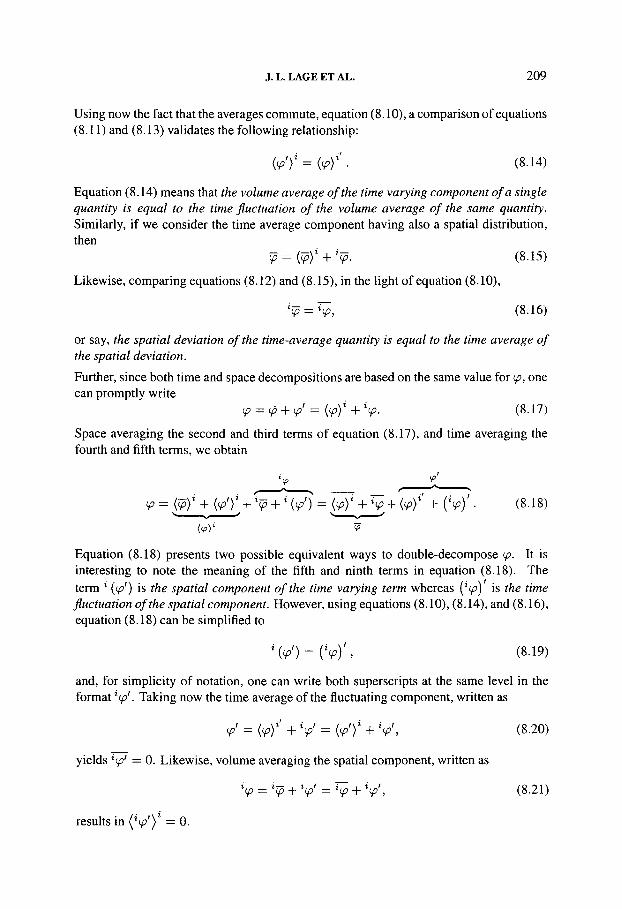
Using now the fact that the averages commute, equation (8.10), a comparison of equations (8.11) and (8.13) validates the following relationship:

i'P'y = ivf • (8-14)

Equation (8.14) means that the volume average of the time varying component of a single quantity is equal to the time fluctuation of the volume average of the same quantity. Similarly, if we consider the time average component having also a spatial distribution, then

^ = ( ^ ) ^ 4 - V . (8.15)

Likewise, comparing equations (8.12) and (8.15), in the light of equation (8.10),

V = V , (8.16)

or say, the spatial deviation of the time-average quantity is equal to the time average of the spatial deviation.

Further, since both time and space decompositions are based on the same value for cp, one can promptly write

^^Tp-\-ip' = {^Y + 'ip. (8.17)

Space averaging the second and third terms of equation (8.17), and time averaging the fourth and fifth terms, we obtain

^-(^r + (^r+v+M^')-(^r+v+(^r +(v) • (8.18) > — ^ — - >—^—^

Equation (8.18) presents two possible equivalent ways to double-decompose ip. It is interesting to note the meaning of the fifth and ninth terms in equation (8.18). The term ^ ((/?') is the spatial component of the time varying term whereas (V) is the time fluctuation of the spatial component. However, using equations (8.10), (8.14), and (8.16), equation (8.18) can be simplified to

^(< '̂) = ( V ) ' , (8.19)

and, for simplicity of notation, one can write both superscripts at the same level in the format V'- Taking now the time average of the fluctuating component, written as

(̂ ' = ((^)^'+V = ((^T + V , (8.20)

yields *(/?' = 0. Likewise, volume averaging the spatial component, written as

V - v + V = V + V', (8.21)

results in (V')^ ~ ^'


With these relationships in mind, integration of local (microscopic) flow governing equations applied to the domain of Figure 8.1 can be more easily treated by using the double-decomposition approach.

Figure 8.2, see Rocamora, Jr and de Lemos (2000a), is helpful in understanding the double-decomposition concept. The figure shows a three-dimensional diagram for a general vector variable (p. For a scalar, all the quantities shown would be drawn on a single line. Also, notice that the points B, C, D and E fall in the same plane, with segments BC and BE parallel to ED and CD, respectively. The path ACF represents the standard space-decomposition given by equation (8.2) whereas equation (8.7) is pictured by the path AEF. Further, equation (8.11) is represented by the path ABC and equation (8.15) by path ABE. Triangles EDF and CDF are associated with equations (8.20) and (8.21), respectively. Equation (8.10) is represented by segment AB and the two equations (8.14) and (8.16) by the equivalence between the parallel segments BC and ED and between segments BE and CD, respectively. Finally, equation (8.18) follows the sequence ABCDF, or the path ABEDF, both of them decomposing the same general variable (p.

Figure 8.2 General three-dimensional vector diagram for a quantity ^p, see Rocamora, Jr and de Lemos (2000a)


8.5 TRANSPORT EQUATIONS

In deriving the time- and space-averaged transport equations for modeling turbulence in porous media, we consider incompressible single-phase flow in a saturated, rigid porous medium. The microscopic continuity equation for a fluid flowing in a clear (of porous medium) domain is given by

V u = 0. (8.22)

Recalling that the fluid speed at the solid-fluid interface is zero, equation (8.4) can be used to take the volume-average of equation (8.22). Then, taking the time-average, equation (8.6), of the resulting equation (recall that the time-integral commutes with the divergent operator) leads to

V • (Ja)^ = 0. (8.23)

One can now take the time-average of equation (8.22), using equation (8.6), and then take the volume-average of the resulting equation using equation (8.4). The result is

V- ((tir)-o, (8.24)

which is exactly the same as equation (8.23), according to equation (8.10). Hence, the averaging order is immaterial for the continuity equation.

If we now expand the velocity field of equation (8.22), using the double-decomposition, equation (8.18), one obtains

V • u = V • (^{uY + {u'Y + % + ^ix') -0. (8.25)

Comparing equation (8.25) and equation (8.24), the divergence of the sum of the last three terms within the parentheses in equation (8.25) must equal zero.

The microscopic momentum equation for a fluid with constant properties is given by the Navier-Stokes equation

du ~dt

-I- V • {uu) -Vp + iJ,V^u-\- pg.

Taking the time-average using u = u-{-u' gives

dt -h V • (uu) = -Wp 4- /iV^n + V • {-pu'u') -h pg,

(8.26)

(8.27)

where the stresses —pu'u' are the well-known Reynolds stresses. On the other hand, the volumetric average of equation (8.26), using equations (8.3) - (8.5), results in

d_

dt ((^(ti) ')-fV-[(/>(uix)']] - - v ( 0 ( j 9 ) ' ) + / i V 2 ( 0 ( t x ) ' ) + ( / > p g + R, (8.28)


where

R= ^ ^ylniS7u)dS-^l^npdS (8.29)

represents the total-drag force per unit volume due to the presence of the porous matrix, being composed by both viscous-drag and form-drag. Further, using equation (8.2) to write u = {uY + ^u in the convective inertia term, one obtains

= - V (</> (p)') + nV^ (0 (u) ' ) - V • [(̂ ( 'u^u)'] + (f>pg + R. (8.30)

Hsu and Cheng (1990) pointed out that the third term on the right-hand side of equation (8.30),V-((/>('«'u)') , represents the hydrodynamic dispersion due to spatial deviations. Note that equation (8.30), closed by replacing R with the viscous-drag (Darcy) term and the form-drag (Forchheimer) term, models typical porous media flow for Rcp < 150-200. However, when extending the analysis to turbulent flow the time varying quantities have to be considered.

The set of equations (8.27) and (8.30) are used when treating turbulent flow in clear fluid or low Rcp porous media flow, respectively. Each one of those equations was derived by applying only one averaging operator, either time or volume, respectively, into the microscopic equation. For modeling turbulent flow in porous media, it is necessary to apply both operators. Hence, the volume average of equation (8.27), giving for the time-mean flow in a porous medium, is given by

= - V (</. {p}') + M V (<A (n) ' ) + V • (^-P4> ( ^ Z V ) ' ) + 4>pg + R, (8.31)

where

f n{Vu)dS--^ f npdS (8.32)

is the time-averaged total-drag force per unit volume, due to the solid matrix, composed of both, viscous-drag and form-drag terms.

Likewise, applying now the time average operation to equation (8.28), one obtains

d p U^ (</. (u -I- w') ') +V-(^<t>{iu + u') {u + « ' ) ) ' )

= - V ((/. (p -I- p ' ) ' ) + MV^ {(t> {u + w')') + # 9 + R (8.33)

J.L.LAGEETAL. 213

Dropping terms containing only one fluctuating quantity results in

d - ( ( A ( t z r ) + V . ( 0 ( ^ u r )

= - V (0 (p)') + /iV^ (0 (tl)^) + V • ( - P 0 (ÎV) ' ) 4- (t>P9 + S , (8.34)

where

=-^ I n(Vu)dS — [ npdS. (8.35)

Comparing equations (8.31) and (8.34) one can see that also for the momentum equation the order of the application of both averaging operators is immaterial as long as the total-drag term is not closed after the volume averaging operation. Pedras and de Lemos (2000a) propose that the term R, appearing in both equations (8.31) and (8.34) (compare equations (8.32) and (8.35)) be modeled by the Hazen-Dupuit-Darcy (HDD) model extension (also known as the Darcy-Forchheimer model). This approach is consistent with the fact that the HDD model seems to correlate experimental data well even when the flow within the pores is turbulent. In other words, the HDD model results from the time and space averaging of the turbulent flow.

Consider now the convective inertia term and the Reynolds stress component of equation (8.31). These two terms can be decomposed using equation (8.15) as follows:

V. [(t> ({uuY + (u^y)] = V • |(/> \{({uy+%) [{uY+%))' + (^?^)'| I = V • {(̂ [{uY {uY + (%%)' 4- {^îJu^y] } .

(8.36)

Now, invoking equation (8.20) to write u' = {u'Y + û'. the term to the right of the equal sign in equation (8.36) becomes

V . [(t> [{uY {uY + Cu'uY + (u'u'Y]}

= vU {uY {uY + (%%)' + ((^{u'Y + û') (^{u'Y + 'u')

- V • {0 [{uY {uY + {'u'uY + {u'Y {u'Y

+ (^{u'Y 'wy -h (^'u' {u'Yy+(^'u'vy i . (8.37)


The fourth and fifth terms on the right-hand side of equation (8.37) are zero because they contain the volume average of one space varying quantity. Equation (8.36) then reduces to

(8.38) V . ((f){uuY^ = V • [0 ({uuY + (u ' t i ' ) ' ) ]

Using the equivalence equations (8.10), (8.14), and (8.16), equation (8.38) can be further simplified into

V • (0 (UUY) - V • I ^ [ ( ^ ( ^ -f {uY' {uY' + / ^ ^ ) ' + (^^T^yl I . (8.39)

Another route to follow is to start with the application of the space decomposition in the convective inertia term, as usually done in classical mathematical treatment of porous media flow analysis, and then follow with the time average. The result is as follows:

= V'[(t)({uY{uY + {'u'uY)]-(8.40)

The time average of the right-hand side of equation (8.40), using equation (8.11) to express {uY = (n)* -f- (TX')\ is given by

V- [(t>({uY{uY + {'u'uY)]

= V'U [({uY + {U'Y) {{UY + {U'Y) + {'UÛY] I (8.41)

- V • {0 [{uY {uY + {u'Y {u'Y + {'U'UY\ }.

With the help of equation (8.21), one can write û = û + û\ and equation (8.41) becomes

V • {0 [{uY {uY + {u'Y {u'Y + {ÛÛY\ }

= V • {(̂ [{uY {uY + {u'Y {u'Y + {{û + V) {m -f 'u')Y\}

= V J 0 {uY {uY + {u'Y {u'Y + Ou'u 4- 'u'u' + 'u'û -h 'u''u'\ \ .

(8.42)

The fourth and fifth terms on the right-hand side of equation (8.42) are zero for containing the time average of one time fluctuating component. In addition, recalling the equivalence


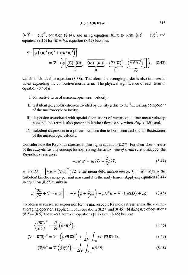
{u'Y — (w)^ , equation (8.14), and using equation (8.10) to write {uf — {u)\ and equation (8.16) for û = û, equation (8.42) becomes

V-[(/)((u)'(Tx)' + (û^n)')]

= V • U\{uy {uY + {u'Y {u'Y + ( % % ) ' 4- {^^^?^y 11, (8.43)

III IV

which is identical to equation (8.38). Therefore, the averaging order is also immaterial when expanding the convective inertia term. The physical significance of each term in equation (8.43) is:

I convective term of macroscopic mean velocity;

II turbulent (Reynolds) stresses divided by density p due to the fluctuating component of the macroscopic velocity;

III dispersion associated with spatial fluctuations of microscopic time mean velocity, note that this term is also present in laminar flow, or say, when Rcp < 150; and,

IV turbulent dispersion in a porous medium due to both time and spatial fluctuations of the microscopic velocity.

Consider now the Reynolds stresses appearing in equation (8.27). For clear flow, the use of the eddy-diffusivity concept for expressing the stress-rate of strain relationship for the Reynolds stress gives

-pvJvJ = iJ,t2D - -pkl, (8.44) o

where D = VtH- (Vil) /2 is the mean deformation tensor, k = u' - u'/2 is the turbulent kinetic energy per unit mass and / is the unity tensor. Applying equation (8.44) in equation (8.27) results in

du ^ . -V (p -f -pk) + ^V^tx + V • {pt2D) -h pg. (8.45)

To obtain an equivalent expression for the macroscopic Reynolds stress tensor, the volume-averaging operator is applied in both equations (8.27) and (8.45). Making use of equations (8.3) - (8.5), the several terms in equations (8.27) and (8.45) become

(Vp)^ = v(<^(p) ' ) + ^ | npdS, (8.48)


(V • wuy = V • {vny + ̂ / ^ (vtz) ds

Equation (8.27) gives further

and equation (8.45)

(V . ( « 2 5 ) ) ' = V . ( / . . .2(B) ' ) + -1^ j „ • (i„2D) AS.

where

= 5 { [v (^ (n)^) + [V (0 (n)^)] "̂ j + ^ / ^ [n« + inu)"] d5}

(8.49)

(8.50)

(8.51)

(8.52)

(8.53)

(8.54)

(8.55)

On noting that at the fluid-soHd interface u = u'u' = fit = k = 0, the equation for the macroscopic momentum equation for turbulent flow in porous media, based on equation (8.27), is given by

p[|(^(n)')+V-(^(«n)')]

= - V (0 (p)') + ^ V (</> («)') + V • (-p.^ (H^y) + (t>pg + H, (8.56)

and based on equation (8.45) is given by

[ I (0(u)^)+V-(0{««)')]

-V (<̂ (^Y + -̂/-P (fc)') + MV^ (<̂ («)') + V • {iit,2 {DY) + ,/>̂ g + R,

(8.57)


where R is given by equation (8.32). Furthermore, the term —p(j){u'u') in equation (8.56) is the macroscopic Reynolds stress tensor. Moreover, the deformation tensor in equation (8.57) is given by

{DY = 1 [V [4>{UY) + [V (^(n)')]^] • (8-58)

A proposal for the macroscopic Reynolds stress tensor can be made by comparing equation (8.56) and (8.57) term by term, namely

-p<i> {ijj^y = fxt,2 (py - ^cj>p {ky i, (8.59)

which is similar to the eddy-diffusivity model for microscopic flow embodied in equation (8.44). However, it should be noted that the coefficient /i^^ appearing in equation (8.59) is defined according to equation (8.54) and is not necessarily the same coefficient used for modeling clear flow, used in equation (8.44). Further, in this work, for simplicity, an

•2

expression of the type /i^^ = pc^ {kY / {sY is used. The macroscopic Reynolds stresses tensor of equation (8.31), modeled herein by equation (8.59), can be further expanded, with the help of the equality u' = {u'Y + ^u'^ as follows:

p0 {u'u'Y = -p(j) {u'Y {u'Y + Ou' 'u'\ (8.60)

The first term on the right-hand side is associated with time fluctuations of the macroscopic mean velocity, whereas the second term represents the turbulent dispersion in porous medium due to both time and spatial fluctuations of the microscopic velocity, see the term IV in equation (8.43).

Also interesting to note is the intrinsic (fluid) average for k, given here as (A:)\ and appearing for the first time in equation (8.52). The turbulence kinetic energy used in Lee and Howell (1987), Wang and Takle (1995), Antohe and Lage (1997), and Getachew et aL

(2000), differs from (kY and is given by km — {u'Y * (^OV^- P̂ ^̂ ^̂ s and de Lemos (2000a), using the double-decomposition approach, derived the relationship between these two quantities, namely

{kY = ^ {^H^^y = ^{u'Y-{u'Y + ^{'u'-'u'Y = km-\-^ ( ^ i x ' - V ) ' . (8.61)

The last term on the right-hand side of equation (8.61) is an extra turbulent kinetic energy term obtained by adding the elements of the main diagonal of the term IV in equation (8.43).


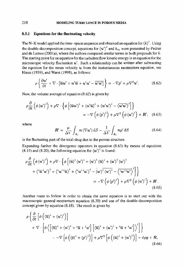
8.5.1 Equations for the fluctuating velocity

The N-K model applied the time-space sequence and obtained an equation for (A:)*. Using the double-decomposition concept, equations for (tx')* and km were presented by Pedras and de Lemos (2001a), where the authors compared similar terms in both proposals for k. The starting point for an equation for the turbulent flow kinetic energy is an equation for the microscopic velocity fluctuation u'. Such a relationship can be written after subtracting the equation for the mean velocity u from the instantaneous momentum equation, see Hinze (1959), and Warsi (1998), as follows:

p < ^ - + V • [uu' + u'u + u'u' - u'u'l > = -Vp' + iJiV'^u'. (8.62)

Now, the volume average of equation (8.62) is given by

p ^ ((/) (txV) + pV • {0 [{uu'Y + {u'uY + {u'u'Y - (^IV) ' ] }

= - V (0 ( P T ) + /iV^ (0 (tx')') + E!, (8.63)

where

R' = - ^ f n {Vu') d5 - - ^ / np' dS (8.64) ^ ^ J A, ^^ JAi

is the fluctuating part of the total-drag due to the porous structure.

Expanding further the divergence operators in equation (8.63) by means of equations (8.15) and (8.20), the following equation for {u'Y is found:

p | (0 («')') + pv • {<A [{uy {u'Y + {u'Y {uY + {ui («')•

+ ( ' « ' « ' ) ' + {'u'%)' + {'u''u'Y - {u'Y {u'Y - (h^^y] I

= -\/[<f>{p'Y)+fiy'{4>{u'Y)+R'. (8.65)

Another route to follow in order to obtain the same equation is to start out with the macroscopic general momentum equation (8.30) and use of the double-decomposition concept given by equation (8.18). The result is given by

+ V • L ([{uY + {u'Y + 'u +'«'] [{uY + {u'Y + %+ '« ' ] ) 1 1

= - V [0 [{PY + {p'Y)] + A'V^ [<!> [{uY + {u'Y)] + 4>P9 + R, (8.66)


which can be simplified to

+ V • [.̂ ((«)' {uY + {uY {u'Y + {u'Y {uY + {u'Y {u'Y

+ {'u'uY + {'u'u'Y + {'u''uY + {'u''u'Y)] I

= -V [0 [{PY + {p'Y)] + MV^ [0 (^{uY + (u'Y)] + cj,pg + R.

(8.67)

Taking now the time average of equation (8.67), one obtains

p I ̂ (</. (UY) + V • !</. huY {uY + {u'Y {u'Y + {'u'uY + (^^7v)'] 11

= - V (<t> (p)') + p V (0 {«)') + <i>pg + R, (8.68)

where

« = ^ / n (Vn) d S ~ ^ l npdS (8.69)

represents the time-averaged value of the instantaneous total-drag given by equation (8.29).

An equation for the fluctuating macroscopic velocity is then obtained by subtracting equation (8.68) from (8.67) and one obtains

p | (0 {ur) -f pv • {0 [{uY {u'Y + {u'Y {uY + {u'Y {u'Y

-f {'u'u'Y + {'u''uY + {'u''u'Y - {u'Y {u'Y - ( V ^ y ] }

(8.70)

Here R' is also given by equation (8.64). Comparing equation (8.70) with equation (8.65) we observe that these two equations are identical.

8.5.2 Equation for turbulence kinetic energy

As mentioned previously, the determination of the flow macroscopic turbulent kinetic energy follows two different paths in the literature. In the A-L method (space-time

averaging sequence) the turbulence kinetic energy is defined as km = {u'Y • {u'Y/'^- On the other hand, the N-K method (time-space averaging sequence) defines the turbulence


kinetic energy as {kY = {u' • u') /2 . The objective of this section is to derive the

transport equation for both, km and (A:)\ and compare the results.

From the instantaneous microscopic continuity equation, equation (8.24), one has

v-(.^(«r)=o. (8.71)

Taking the scalar product of equation (8.63) and ( u ' ) \ using equation (8.71) and time averaging the result, an equation for k^ is developed, having the following terms:

p(n')'-|(0(«f)=P d {<t>km)

dt ••

p{u'Y-[v-(4>{u'u')^}

= p{u'Y • {V • U {uf {u'Y + ̂ (^IZ'«')1}

= pV-[4> {uY km] + p{u'Y • {V • [0 ('n'«')'] },

(8.72)

(8.73)

p{u'Y-[v-(j>{u'u'Y)]

= p{u'Y • {V • [0 {u'Y {uY + 0 {'W 'u)*l}

= pcPiu'Y {u'Y : V {uY + p{u'Y • {V • [</) {iu' iuY] },

p{u'Y-{v-{4>{u'u'Y)}

= p{u'Y • {V • U {u'Y {u'Y + 4> {'w iu'Y]}

i {u'Y-{u'Y 4>{u) + p{u'Y -{y • U(^it''it')']},

p{u'Y-{v •[-<!> {u'u'y)} = Q, -(nf • V (0 (p')') =-V • [0 («f (P'r),

tx{u'Y • V2 ( 0 (« ' ) ' ) = M V ' {<j>km) - P<l>Sr,

{u'Y -R' = Q,

(8.74)

(8.75)

(8.76)

(8.77)

(8.78)

(8.79)

where Sm = ''V {u'Y ' (V {u'Y) • In handling equation (8.77) the porosity 0 was assumed to be constant only for simplifying the manipulation to be shown next. However,


this procedure does not represent a limitation in deriving a general transport equation for km since equation (8.77) requires further modeling.

Another important point is the treatment given to the scalar product shown in equation (8.79). Here, a different view from the work in Lee and Howell (1987), Wang and Takle (1995), Antohe and Lage (1997), and Getachew et al (2000), is considered. The fluctuating drag form R' acts through the solid-fluid interfacial area and, as such, on fluid particles at rest. The fluctuating mechanical energy represented by the operation in equation (8.79) is not associated with any fluid particle movement and, therefore, is here considered to be zero.

A final equation for km gives

d{(t)km) ^ dt

pV • ^(j) {uY kmj

= -pV'{cj>{ur {p'Y ^ {u'Y'{u'Y (8.80)

+ / i V ' ( # ^ ) - p(l){u'Y {U'Y ' V {uY - P(t>£m - Dr,

where

Dm - p{u'Y • {V • [0 [{ûû'Y + {'W ûY + {'W û' )^)] } (8.81)

represents the dispersion of km given by the last terms on the right-hand side of equations (8.73), (8.74) and (8.75). It is of interest to point out that this term can be either negative or positive.

The first term on the right-hand side of equation (8.80) represents the turbulent diffusion of km and is normally modeled via a diffusion-like expression resulting for the transport equation for km. see Antohe and Lage (1997) and Getachew et al (2000), as follows:

p ^ m + pv dt

<t>{uYkm}^

= V + Pm - P<f>£n Dr.

where Pm = -pckiu'Y {U'Y : V {uY

(8.82)

(8.83)

is the production rate of km due to the gradients of the macroscopic time-mean velocity {uY.

The A-L model uses the above equation for km considering R' as the HDD (Darcy-Forchheimer) model with macroscopic time-fluctuation velocities (u'Y- The mode also does not include all dispersion terms that were here grouped into Dm equation (8.81). It should be noted that the averaging order in this case does matter.

The other procedure for composing the turbulence kinetic energy is to take the scalar product of equation (8.62) by the microscopic fluctuating velocity u'. Then apply both time


and volume averaging operators for obtaining an equation for (fc)* = {u' • u') / 2 . It is worth noting that in this case the order of application of both operations is immaterial since no additional mathematical operation is conducted in the averaging processes. Therefore, this is the same as applying the volume operator to an equation for the microscopic k.

The volume average of a transport equation for k has been carried out in detail by de Lemos and Pedras (2000a) and Pedras and de Lemos (2001a). Only the final resulting equation is presented here, namely

d_

dt (ct>{k)')+V'{uD{k)')

= V . + ^)v (*«- ) (8.84)

-\-Pi + Gi-p(t){e)\

where

Pi = -p{u'u'y : VUD,

{ky\uD\ Gi = Ckp(t>-

VK

(8.85)

(8.86)

are the production rate of {kY due to mean gradients of the seepage velocity and the generation rate of intrinsic k due the presence of the porous matrix.

A comparison between terms in the transport equation for km and {kf can now be conducted. Expanding the correlation forming the production term Pi by means of equation (8.2), a connection between the two generation rates can also be written as

Pi = -p{u'u') : VUD

-p ([u'Y {u'Y : VUD + {'W'u'Y : V U D ) (8.87)

^ Pm - P{'U''U'Y • ^UD-

One can note that all the production rate of km due to the mean flow constitutes only part of the general production rate responsible for maintaining the overall level of {kY -

The dissipation rates also carry a similar correspondence if one expands

{sY = V (Vu' : {Vu'f

(8.88)


Considering further constant porosity,

{sY ^em^y[' (VtxO : ' {Vu'f) . (8.89)

This indicates that an additional dissipation rate is necessary to fully account for the energy decay process inside the REV.

8.6 MACROSCOPIC MODEL ADJUSTMENT

Pedras and de Lemos (2000b, 2001b, 2001c) performed numerical simulations on periodic REV cells, with the solid matrix represented by cylindrical, longitudinal and transversal elliptic rods. These simulations were used to calibrate the Pedras and de Lemos turbulence model. The microscopic (pore level) flow equations were numerically solved inside an elementary REV. In all cases, a periodic boundary condition was imposed along the axial direction. The Reynolds number Ren based on the cell height H was varied from about 0.35 (creeping flow) to L2 x 10^ (fully turbulent regime). A version of the k-e model for low Re flow was also incorporated in the code, following the damping functions presented by Abe et al. (1997). The non-orthogonal grid was based on a generalized coordinate system, leading to a total of 150 by 100 irregular control volumes for the high Re model and 300 by 200 for the low Re cases. Samples of the numerical grid are shown in Figure 8.3. For Ren = 12 x 10^, both k-e models were calculated for comparison.

The numerical method SIMPLE was employed for relaxing the mean and turbulence equations within the domain. The dimensions of the periodic cell for the cases considered were i? = 0.1m, 5 = 2iJ, D = 0.03 m (0 = 0.8), 0.05 m (0 = 0.6) and 0.06 m ((/) = 0.4). The solutions were grid independent and all normalized residuals were reduced to 10~^. Also, relaxation parameters for all variables were kept equal to 0.8. A summary of all relevant parameters for the circular rod case is presented in Table 8.1. The constant Ck introduced in the equation for {k)\ via equation (8.86), was determined for closure of the macroscopic mathematical model proposed by Pedras and de Lemos (2001a). In that work, a methodology was devised in order to obtain such value. Accordingly, the need of computing the fine flow properties in order to obtain the volume-integrated quantities has motivated the development of adequate numerical tools. As mentioned, those calculations were needed for adjusting the model and considered either the high Re k-e closure, Rocamora, Jr and de Lemos (1998), as well as the low Reynolds version, Pedras and de Lemos (2001b). Heat transfer analysis was also the subject of additional research, Rocamora, Jr and de Lemos (1999). One of the outcomes of this development was the ability to treat hybrid computational domains with a single numerical tool, Rocamora, Jr and de Lemos (2000b, 2000c).

For macroscopic fully developed uni-dimensional flow in isotropic and homogeneous media the limiting values for {kY and {eY in the additional terms introduced in equation (8.84) and its accompanying equation for {eY (not shown here) are given the values k(f, and e<p, respectively. In this limiting condition, the transport equations for {kY and {eY


(a)

(b)

H

2H

(c)

H

2H

Figure 8.3 Model of REV, periodic cell and elliptically generated grids: (a) cylindrical rods, (b) longitudinal elliptical rods, and (c) transverse elliptical rods. See Pedras and de Lemos (2001c)

reduce to

{ey = ck {kr\uD\ {sY

VK ' {ky = Cfc

VK (8.90)

Using the limiting cases k^ and e^, the pair of equations (8.90) can be combined into the non-dimensional form

E^sfK ki,

I «D I C f c — - [ 2 -

\UD\ (8.91)


Table 8.1 Parameters for microscopic computations (speeds in m/s)

Ren 1.20 x 10^ 1.20 x 10^ 1.20 x 10^ 1.20 x 10^ 1.20 x 10^

) = 0.4 1.80 X 10^ 1.80 X 10° 1.80 X 10^

4.50 X 10^ uu 1 .80x10- '^ 1 .80x10- _ _ _ . . _ _ (n)* 4.50 X 10"^ 4.50 x 10"^ 4.50 x 10° 4.50 x 10°

"^D 1.79 x lO- ' * 1 .79x10-1 1 .79x10° 1 .79x10° 1,79 x 10^ {uY 2.99 X 10-^ 2.99 x 10"! 2.99 x 10° 2.99 x 10° 2.99 x 10^

"^D 1 . 7 9 x 1 0 - ^ 1 .79x10-1 1 .79x10° 1 .79x10° 1.79 x 10^ ~ ' {uf 2.24 X 10-^ 2.24 x 10-^ 2.24 x 10° 2.24 x 10° 2.24 x 10^

Turbulence model

Laminar Low Re Low Re High Re High Re

The permeability used in equation (8.91) was calculated by solving the flow equations for all three geometries and for the Darcy regime (creeping flow, Reu < 1). In order to obtain Ck, the microscopic computations described above for different porosity and Ren were used to calculate the corresponding limiting values fc^ and £0. Once these intrinsic values were obtained, then they were plugged into equation (8.91). The value 0.28 found for Ck from Figure 8.4 correlates very well the data.

|UDI

1.2

1.0

0.8

0.6

^ Transversal ellipses 1 ^ , , , , ,^^^, ^ '^ > Pedras and deLemos (2001c)

A Longitudinal ellipses D Pedras and de Lemos (2001 a) O Nakayama and Kuwahara (1999)

I I I I 1 I I I I I I I I

Figure 8.4 Determination of the Ck value from the best fit using \UD\ = Ckkcf,/ \UD\ for different geometry, porosity and Reynolds

number See Pedras and de Lemos (2001c)

226 MODELING TURBULENCE IN POROUS MEDU

8.7 CONCLUSIONS

One can establish a general classification of the turbulence methods presented in the literature based on the sequence of application of averaging operators, on the handling of surface integrals and on the applications reported so far. A summary of this classification is presented in Table 8.2.

The A-L method derives the transport equations for km instead of {k)\ The initial model, based on this method, and developed by Antohe and Lage (1997), was refined by Getachew et al. (2000). This method is based on time-averaging to macroscopic (volume-averaged) equations.

Table 8.2 Classification of turbulence models fi)r porous media (from de Lemos and Pedras, 2001)

References General characteristics Integration Applications

A-L Lee and Howell (1987), Wang and Takle (1995), Antohe and Lage (1997), Getachew et al. (2(X)0).

Surface integrals are not applied since models are based on macroscopic quantities subjected to time-averaging only.

Space-time Only theory presented. Numerical results using this model are found in Chm etal. (2000).

N-K Masuoka and Takatsu (1996), Kuwahara ^r a/. (1998), Takatsu and Masuoka (1998), Nakayama and Kuwahara (1999).

Masuoka and Takatsu (1996) assumed a non-null value in their equation (11) for the turbulent shear stress St — —pu'u' along the interfacial area Ai. Takatsu and Masuoka (1998) assumed in equation (14) a different from zero value for d = {fi/p + p^t/cTkp) V/c at the interface Ai.

Time-space Microscopic computations on periodic cells of square rods. Macroscopic model computations presented.

T-C Travkin and Catton (1994, 1995, 1998), Catton and Travkin (1996), Gr2Mon etal. (1996), Travkin e/fl/. (1999).

Morphology-based theory. Surface integrals and volume-average operators depend on media morphology.

Time-space Only theory. No closure for the macroscopic equations is presently available.

P-dL Pedras and de Lemos (2000a), Rocamora, Jr and de Lemos (2000a), Pedras and de Lemos (2001a, 2001b).

Double-decomposition theory. Surface integrals involving null quantities at surfaces are neglected. The connection between space-time and time-space theories is unveiled.

Time-space Microscopic computation on periodic cell of circular and elliptical rods and for hybrid domains are found in de Lemos and Pedras (2000b), Rocamora, Jr and de Lemos (2000b, 2000c).


In this sense, the sequence space-time integration is employed and surface integrals are not manipulated since macroscopic quantities are the sole independent variables used. As stated so precisely in the abstract of Antohe and Lage (1997)

Turbulence models derived from the [A-L method] . . . will inevitably fail to characterize accurately turbulence induced by the porous matrix in a microscopic sense [at the pore level].

Application of this theory is found in Chan et al. (2000).

The N-K method constitutes the second class of models here compiled. It is interesting to mention that Masuoka and Takatsu (1996), when deriving their model based on the N-K method, assumed a non-null value for the turbulent shear stress, St = -pu'u', along the interfacial area in their equation (8.11). With that, their surface integral jj^ St-ndA was associated with the Darcy flow resistance term. Yet, using the Boussinesq approximation as in their equation (8.7), St — 2^tD - \kl, one can see that both /i^ and k will vanish at the surface Ai, ultimately indicating that the surface integral in question is actually equal to zero. Similarly, Takatsu and Masuoka (1998) assumed for their surface integral in equation (8.14), / ^ d • n dA, a non-null value, where d — {/j>/p + pt/c^kP) VA:. Here,

it is worth noting also the identity VA: = u' • [Vu') . Moreover, at the interface Ai we have VA: = 0 due to the no-slip condition. Consequently, the surface integral of d over Ai is zero. In regard to the average operators used, the N-K method follows the time-space integration sequence. Calibration of models derived following the N-K method is possible for microscopic computations on a periodic cell, see Nakayama and Kuwahara (1999).

The work developed in a series of papers using a morphology-oriented theory is here grouped under the T-C method. In this morphology-based theory, surface integrals resulting after application of volume-average operators depend on the media morphology. The governing equations set up for turbulent flow, although complicated at first sight, just follow the usual volume integration technique applied to the standard k-e and k-L turbulence models. In this sense, the time-space integration sequence is followed. No closure is proposed for the unknowns surface integrals (and morphology parameters) so that practical applications of such development in solving practical engineering problems is still a challenge to be overcome.

Finally, the P-dL method uses the double-decomposition theory. The connection between space-time and time-space averaging models is made possible due to the splitting of the dependent variables into four (rather that two) components. For the momentum equation, the averaging order is immaterial (as long as the closure for the total-drag is done only after the averaging operators are applied). For the turbulence kinetic energy equation, however, the order of application of such mathematical operators will lead to different quantities being transported. Results for hybrid domains (porous medium-clear flow) are found in de Lemos and Pedras (2000b), and Rocamora, Jr and de Lemos (2000b, 2000c, 2000d).


Acknowledgements

MJSdL is thankful to CNPq, Brazil, for the financial support during the preparation of this work. The numerical simulations by Marcos H. J. Pedras and Francisco D. Rocamora, Jr were performed as part of their doctoral dissertation work at ITA. The authors acknowledge the opportunity, given by the editors, to work out their initially different technical opinions on many issues through informal, collegial communications and present their common views in this unique chapter.

REFERENCES

Abe, K., Nagano, Y, and Kondoh, T. (1997). An improved k-e model for prediction of turbulent flows with separation and reattachment. Trans. Japanese Soc. Mech. Eng. B58:554, 3003-3010.

Antohe, B. V. and Lage, J. L. (1997). A general two-equation macroscopic turbulence model for incompressible flow in porous media. Int. J. Heat Mass Transfer 40, 3013-3024.

Bear, J. (1972). Dynamics of Fluids in Porous Media. Elsevier, New York.

Catton, I. and Travkin, V. S. (1996). Turbulent flow and heat transfer in high permeability porous media. In Proceedings of the International Conference On Porous Media and their Applications in Science, Engineering and Industry, Kona, Hawaii (ed. K. Vafai), pp. 333-368. Engineering Foundation, New York.

Chan, E. C , Lien, F.-S., and Yovanovich, M. M. (2(X)0). Numerical study of forced flow in a back-step channel through porous layer. In Proceedings of 34th ASME-National Heat Transfer Conference, Pittsburgh, Pennsylvania. ASME-HTD-I463CD, paper NHTC2000-12118 (on CD-ROM).

de Lemos, M. J. S. and Pedras, M. H. J. (2000a). Modeling turbulence phenomena in incompressible flow through saturated porous media. In Proceedings of 34th ASME-National Heat Transfer Conference, Pittsburgh, Pennsylvania. ASME-HTD-I463CD, paper NHTC2000-12120 (on CD-ROM).

de Lemos, M. J. S. and Pedras, M. H. J. (2000b). Simulation of turbulent flow through hybrid porous medium-clear fluid domains. In Proceedings of the IMECE2000 ASME International Mechanical Engineering Congress and Exposition, Orlando, Florida. ASME-HTD-366-5, pp. 113-122.

de Lemos, M. J. S. and Pedras, M. H. J. (2001). Recent mathematical models for turbulent flow in saturated rigid porous media. / Fluids Eng. 123. To appear.

Dybbs, A. and Edwards, R. V. (1984). A new look at porous media fluid mechanics—Darcy to turbulent. In Fundamentals of Transport Phenomena in Porous Media (eds J. Bear and M. Y Corapcioglu), pp. 199-256. Martinus Nijhoff, Amsterdam.

Getachew, D., Minkowycz, W. J., and Lage, J. L. (2000). A modified form of the k-e model for turbulent flow of an incompressible fluid in porous media. Int. J. Heat Mass Transferals, 2909-2915.

Gratton, J. L., Travkin, V. S., and Catton, I. (1996). Influence of morphology upon two-temperature statements for convective transport in porous media. J. Enhanced Heat Transfer 3, 129-145.

Gray, W. G. and Lee, P C. Y (1977). On the theorems for local volume averaging of multiphase system. Int. J. Multiphase Flow 3, 333-340.

Hinze, J. O. (1959). Turbulence. McGraw-Hill, New York.


Hsu, C. T. and Cheng, P. (1990). Thermal dispersion in a porous medium. Int. J. Heat Mass Transfer 33, 1587-1597.

Kuwahara, F , Kameyama, Y, Yamashita, S., and Nakayama, A. (1998). Numerical modeling of turbulent flow in porous media using a spatially periodic array. / Porous Media 1, 47-55.

Lage, J. L. (1998). The fundamental theory of flow through permeable media from Darcy to turbulence. In Transport Phenomena in Porous Media (eds D. B. Ingham and I. Pop), pp. 1-30. Pergamon, Oxford.

Lage, J. L. and Antohe, B. V. (2000). Darcy's experiments and the deviation to nonlinear flow regime. ASMEJ. Fluids Eng. Ill, 619-625.

Lee, K. and Howell, J. R. (1987). Forced convective and radiative transfer within a highly porous layer exposed to a turbulent external flow field. In Proceedings of the 2nd ASME/JSME Thermal Engineering Joint Conference, Vol. 2, pp. 377-386.

Masuoka, T. (1999). Some aspects of fluid flow and heat transfer in porous media. In Proceedings of 5th ASME/JSME Joint Thermal Engineering Conference, San Diego, California. AJTE99-6304, pp. 1-14.

Masuoka, T. and Takatsu, Y (1996). Turbulence model for flow through porous media. Int. J. Heat Mass Transfer 39, 2803-2809.

Nakayama, A. and Kuwahara, F (1999). A macroscopic turbulence model for flow in a porous medium. ASMEJ Fluids Eng. Ill, 427-433.

Nield, D. A. (1991). The limitations of the Brinkman-Forchheimer equation in modeling flow in a saturated porous medium and at an interface. Int. J. Heat Fluid Flow 12, 269-272.

Nield, D. A. (1997). Conmients on 'turbulence model for flow through porous media'. Int. J. Heat Mass Transfer 40, 2449.

Nield, D. A. (2001). Alternative models of turbulence in a porous medium, and related matters. ASME J. Fluids Eng. In press.

Nield, D. A. and Bejan, A. (1999). Convection in Porous Media (2nd edn). Springer-Verlag, New York.

Pedras, M. H. J. and de Lemos, M. J. S. (1999). On volume and time averaging of transport equations for turbulent flow in porous media. In Proceedings of 3rd ASME/JSME Joint Fluids Engineering Conference, San Francisco, California. ASME-FED-248, paper FEDSM99-7273 (on CD-ROM).

Pedras, M. H. J. and de Lemos, M. J. S. (2000a). On the definition of turbulent kinetic energy for flow in porous media. Int. Comm. Heat Mass Transfer 11, 211-220.

Pedras, M. H. J. and de Lemos, M. J. S. (2000b). Numerical solution of turbulent flow in porous media using a spatially periodic cell and the low reynolds k-e model. In Proceedings of the CONEM2000— National Mechanical Engineering Congress, Natal, Brazil, (on CD-ROM, in Portuguese).

Pedras, M. H. J. and de Lemos, M. J. S. (2001a). Macroscopic turbulence modeling for incompressible flow through undeformable porous media. Int. J. Heat Mass Transfer 44, 1081-1093.

Pedras, M. H. J. and de Lemos, M. J. S. (2001b). Simulation of turbulent flow in porous media using a spatially periodic array and a low Re two-equation closure. Numer Heat Transfer, Part A 39, 35-59.

Pedras, M. H. J. and de Lemos, M. J. S. (2001c). Computation of turbulent flow in porous media using a low reynolds k-£ model and an infinite array of spatially periodic elliptic rods. Numer Heat Transfer, Part A. Submitted.


Rocamora, Jr, F. D. and de Lemos, M. J. S. (1998). Numerical solution of turbulent flow in porous media using a spatially periodic array and the k-e model. In Proceedings of the ENCIT98—7th Brazilian Congress Thermal Sciences, Rio de Janeiro, Brazil, Vol. 2, pp. 1265-1271.

Rocamora, Jr, F. D. and de Lemos, M. J. S. (1999). Simulation of turbulent heat transfer in porous media using a spatially periodic cell and the k-e model. In Proceedings of the COBEM99—15th Brazilian Congress of Mechanical Engineering, Sao Paulo, Brazil, (on CD-ROM).

Rocamora, Jr, F. D. and de Lemos, M. J. S. (2000a). Analysis of convective heat transfer for turbulent flow in saturated porous media. Int. Comm. Heat Mass Transfer 27, 825-834.

Rocamora, Jr, F D. and de Lemos, M. J. S. (2000b). Prediction of velocity and temperature profiles for hybrid porous medium-clean fluid domains. In Proceedings CONEM2000—National Mechanical Engineering Congress, Natal, Brazil, (on CD-ROM).

Rocamora, Jr, F. D. and de Lemos, M. J. S. (2000c). Laminar recirculating flow and heat transfer in hybrid porous medium-clear fluid computational domains. In Proceedings of 34th ASME—National Heat Transfer Conference, Pittsburgh, Pennsylvania. ASME-HTD-I463CD, paper NHTC2000-12317 (on CD-ROM).

Rocamora, Jr, F D. and de Lemos, M. J. S. (2000d). Heat transfer in suddenly expanded flow in a channel with porous inserts. In Proceedings of the IMECE2000 ASME International Mechanical Engineering Congress and Exposition, Orlando, Florida. ASME-HTD-366-5, pp. 191-195.

Slattery, J. C. (1967). Flow of viscoelastic fluids through porous media. Amer Inst. Chem. Eng. J. 13, 1066-1071.

Takatsu, Y. and Masuoka, T. (1998). Turbulent phenomena m flow through porous media. J. Porous Media 1,243-251.

Travkin, V. S. and Catton, I. (1994). Turbulent transfer of momentum, heat and mass in a two-level highly porous medium. In Heat Transfer, 1994: Proceedings International Heat Transfer Conference, Brighton, UK, Vol. 6, pp. 399-^04. Institute Chemical Engineers, Rugby, UK.

Travkin, V. S. and Catton, I. (1995). A two-temperature model for turbulent flow and heat transfer in a porous layer. ASME J. Fluids Eng. 117, 181-188.

Travkin, V. S. and Catton, I. (1998). Porous media transport descriptions—non-local, linear and nonlinear against effective thermal/fluid properties. Adv. Colloid Interface Sci. 11, 389-443.

Travkin, V. S., Hu, K., and Catton, I. (1999). Turbulent kinetic energy and dissipation rate equation models for momentum transport in porous media. In Proceedings of 3rd ASME/JSME Joint Fluids Engineering Conference, San Francisco, California. FEDSM99-7275, pp. 1-7.

Wang, H. and Takle, E. S. (1995). Boundary-layer flow and turbulence near porous obstacles. Boundary-Layer Meteorol 74, 73-88.

Warsi, Z. U. A. (1998). Fluid Dynamics—Theoretical and Computational Approaches (2nd edn). CRC Press, Boca Raton.

Whitaker, S. (1969). Advances in theory of fluid motion in porous media. Ind. Eng. Chem. 61, 14-28.

Whitaker, S. (1999). The Method of Volume Averaging. Kluwer, Dordrecht.

transport phenomena in porous media ii || modeling turbulence in porous media

Documents