topographic survey of the control points for ... · topographic survey of the control points for...

TOPOGRAPHIC SURVEY OF THE CONTROL POINTS FOR PHOTOGRAMMETRIC RECORD

Alex SORIA MEDINA*, Sílvio Jacks dos Anjos GARNÉS**, Simone da SILVA***

Universidade Federal do Paraná Curso de Pós-graduação em Ciências Geodésicas

* [email protected] **Universidade para o Desenvolvimento do Estado e da Região do Pantanal

[email protected] *** Departamento de Desenho

[email protected]

KEY WORDS: Architecture, Control points, Topographical survey. ABSTRACT T he acco mp l i shment o f a p ho to grammet r i c r eco rd ing o f h i s to r i ca l mo nument s i t i s imp o r t an t t ha t be done a topograph ica l su rvey, wi th the purpose o f de t e rmine so me con t ro l po in t s i n the bu i ld ing s t r uc tu r e , fo r pos t e r io r o r i en ta t io n o f t he pho tographs . T h i s pape r shows the expe r i ence o f t he topograph ica l su rvey made in the “So la r do Ro sá r io” , h i s to r i ca l mo nument o f Cur i t i b a – P a raná - B raz i l . T he used me tho d was the sp a t i a l i n t e r sec t io n and the p o in t s co nf igura t io n o f t he b ase (un t i l t o t h r ee p o in t s ) had the i r l o ca t io n d e f ined co nc i l i a t i ng the ava i l ab l e sp ace and the r i g id i t y . T he r edund an t obse rva t ions p rov ided l ea s t sq ua re s ad j us tment . T he f ina l r e su l t s and the r e sp ec t ive accuracy o f t he ad j us tment a l l o wed the i r co mp ar i so n wi th the o b ta ined so lu t io n us ing s imp le r me tho d s , i nd ica t ing the mo re v i ab le i n sp end t ime and accuracy. T he survey was done wi th a t o t a l s t a t i on whose angula r accuracy i s o f 1 ” and l i nea r o f 1 mm + 1 p p m. I t was a l so t r i ed to t e s t t he v i ab i l i t y i n execu t ing the survey wi th eq u ip ment o f sma l l e r co s t , i n t he case a t heo d o l i t e e l ec t ro n ic o f angula r a ccuracy o f 10” .

1 INTRODUCTION

T his wo rk i s o ne s t ep s o f t he p ho to grammet r i c r eco rd ing o f a r ch i t ec tu r a l facad es tha t i s b e ing acco mp l i shed in the " So la r d o Ro sá r io " , co ns t ruc t io n tha t b e lo ngs to the h i s to r i ca l co l l ec t io ns o f Cur i t i b a - B raz i l . T he wo rk i s b e ing d eve lo p ed a t t he P o s t -Grad ua te P ro gram in Geo d es i c Sc iences o f t he Fed e ra l Unive r s i ty o f P a r aná (UFP R) , and th i s s t ep had the suppo r t o f t he Ca l ib r a t io n and Geode t i c I ns t rumenta t io n Labo ra to ry o f UFPR. As we l l a s i n t he co nven t io na l p ho to grammet r i c ( ae r i a l ) , t he t e r r e s t r i a l p ho to grammet r i c i s ba se on con t ro l po in t s t o pho to s o r i en ta t io n , a s we l l a s t o r ep re sen t t he ob j ec t i n a p ro j ec t io n sys t em. T he d e t e rmina t io n o f t hese p o in t s co o rd ina t e s , i n t h i s wo rk , we re ca l cu la t ed by d i f fe r en t me thods us ing topograph ica l obse rva t io ns tha t we re ob ta ined in two f i e ld surveying : i n t he f i r s t , a t o t a l s t a t i o n was used , and in t he seco nd an e l ec t ro n ic t heo d o l i t e .

2 EQUIPMENT AND PROCEDURES

2.1 Equipment

In the d i r ec t io ns o b se rva t io n two eq u ip ment were used in d i f fe r en t su rveying , neve r the le ss occupying the same base s t a t io ns : a t o t a l s t a t io n Le ica T C 2002 , wi th a p r i sm in the ba se measure and an Le i ca e l ec t ron i c t heodo l i t e (T 100) , wi th a t ape measure fo r t he base d e t e rmina t io n . T he sp ec i f i ca t io ns o f b o th ins t rument s a r e sho wn in the t ab le 1 .

Soria Medina, Alex

International Archives of Photogrammetry and Remote Sensing. Vol. XXXIII, Part B5. Amsterdam 2000.734

N e s t o r d e C a s t r o p a

Ro

sá

rio

st r

ee

t

S o l a r d o R o s á r i o

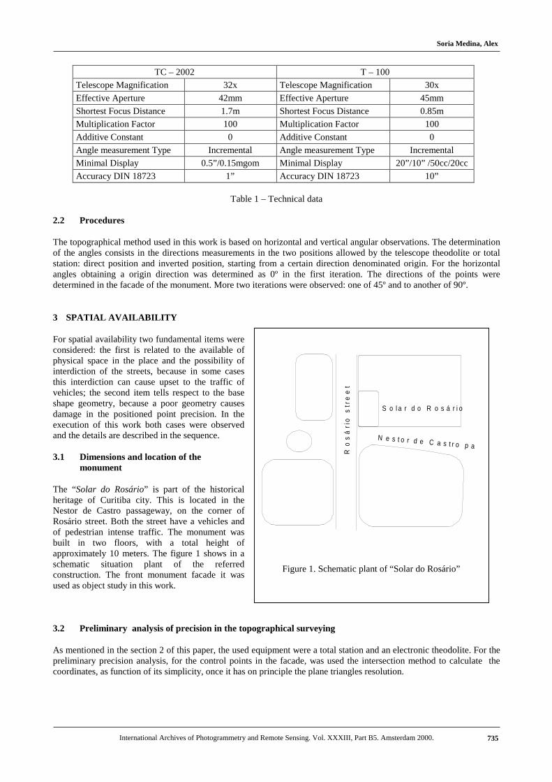
Figure 1. Schematic plant of “Solar do Rosário”

TC – 2002 T – 100

Telescope Magnification 32x Telescope Magnification 30x

Effective Aperture 42mm Effective Aperture 45mm

Shortest Focus Distance 1.7m Shortest Focus Distance 0.85m

Multiplication Factor 100 Multiplication Factor 100

Additive Constant 0 Additive Constant 0

Angle measurement Type Incremental Angle measurement Type Incremental

Minimal Display 0.5”/0.15mgom Minimal Display 20”/10” /50cc/20cc

Accuracy DIN 18723 1” Accuracy DIN 18723 10”

Table 1 – Technical data

2.2 Procedures

The topographical method used in this work is based on horizontal and vertical angular observations. The determination of the angles consists in the directions measurements in the two positions allowed by the telescope theodolite or total station: direct position and inverted position, starting from a certain direction denominated origin. For the horizontal angles obtaining a origin direction was determined as 0º in the first iteration. The directions of the points were determined in the facade of the monument. More two iterations were observed: one of 45º and to another of 90º.

3 SPATIAL AVAILABILITY

For spatial availability two fundamental items were considered: the first is related to the available of physical space in the place and the possibility of interdiction of the streets, because in some cases this interdiction can cause upset to the traffic of vehicles; the second item tells respect to the base shape geometry, because a poor geometry causes damage in the positioned point precision. In the execution of this work both cases were observed and the details are described in the sequence. 3.1 Dimensions and location of the

monument

The “Solar do Rosário” is part of the historical heritage of Curitiba city. This is located in the Nestor de Castro passageway, on the corner of Rosário street. Both the street have a vehicles and of pedestrian intense traffic. The monument was built in two floors, with a total height of approximately 10 meters. The figure 1 shows in a schematic situation plant of the referred construction. The front monument facade it was used as object study in this work. 3.2 Preliminary analysis of precision in the topographical surveying

As mentioned in the section 2 of this paper, the used equipment were a total station and an electronic theodolite. For the preliminary precision analysis, for the control points in the facade, was used the intersection method to calculate the coordinates, as function of its simplicity, once it has on principle the plane triangles resolution.

Soria Medina, Alex

International Archives of Photogrammetry and Remote Sensing. Vol. XXXIII, Part B5. Amsterdam 2000. 735

FAC A D E

BA SEE D

5 6

Figure 2. – Triangle configuration of the processing points

Of the errors theory, it’s known that is smaller the errors observational propagation, if an equilateral triangle was formed. In a practical surveying it is not possible to form equilateral triangles, as it could be observed in the case shown in the “Solar do Rosário”. The figure 2 shows the configuration of the two worse points (with poor geometry). The size of the base B and the distance of this to the facade were determined in agreement with the available space of the place. It was used in this work a local coordinates system, the Cartesian origin of X, Y, Z was established in the instrument optic center, in the E point. The X axis was defined by the ED direction, the Z axis coincident with the vertical of the station E and the Y axis was determined forming a dextrogery system. The measured angles from the E station were called just

for Ê , the angles from the D station were called D , and

the vertical angles were called Z . The following expressions were used calculate the coordinates:

)DE180sec(cosEcosDBsinx −−=�

(3.2.1)

)DE180sec(cosEsinDBsiny −−=�

(3.2.2)

)DE180sec(cosZgcotDBsinz −−=�

(3.2.3)

The covariance matrix ( ∑ bL ) of the observed angles

and of the base is known and the propagation of the covariance law (exp. 3.2.5) provides the covariance matrix of the coordinates (x, y, z) of the points.

∑ ∑=zyxT

LbDD,, (3.2.5)

where:

∂∂

∂∂

∂∂

∂∂

∂∂

∂∂

∂∂

∂∂

∂∂

∂∂

∂∂

∂∂

=

Z

z

D

z

E

z

B

zZ

y

D

y

E

y

B

yZ

x

D

x

E

x

B

x

D

ˆˆˆ

ˆˆˆ

ˆˆˆ

Considering the standard deviation as:

mB 001,0=σ and rad1098481368110,4 6ZDE

−×=σ=σ=σ

The obtained deviations for the coordinates points 5 and 6 were: Point 5 Point 6

=Xσ 0.00241 mm =Xσ 0.00062 mm

=yσ 0.01391 mm =yσ 0.01359 mm

=σz 0.00159 mm =σz 0.00160 mm

Soria Medina, Alex


P

B

dE Dd

E

E

D

D

x

y

γ

P

E

Z

z

E

E

d

Figure 3 – Intersection Method

The deviations above are estimate of the errors for the points positioning in the facade, and they are inside of an acceptable precision. This fact confirms that used configuration to the surveying was appropriate.

4 COORDINATES PROCESSING

T he coo rd ina te s p rocess ing was made us ing th r e e d i f fe r e n t me tho d o lo g ie s : i n t e r sec t io n ; ana lyt i ca l sp a t i a l i n t e r sec t io n ; and l eas t sq ua re s me thod . 4.1 Intersection

T his me tho d co ns i s t s i n the r e so lu t io n o f p l ane t r i ang le s , t o o b ta in the p l ane co o rd ina t e s ( x , y) , a s we l l a s , t he coo rd ina te ( z ) . Be ing E and D two ob se rva t io n s t a t io ns and P the p o in t o f coo rd ina te s to be de te rmine , t he f igure 3 shows the p rocedure . I n the survey were obse rved the

ho r i zon ta l ang le s ( E and D ) , t he ba se B and the ve r t i ca l ang le (Z) fo r e ach s t a t io ns . T he ang le γ was d e t e rmined th ro ugh r e l a t io nsh ip amo ng in t e rna l ang le s o f t he p l ane t r i ang le :

)DE(180 +−=γ�

(4.1.1)

T he d i s t ances d E and d D were ca l cu la t ed ap p lying the s inus l aw:

γ=

sen

DsenBd E

( 4 . 1 . 2 )

γ=

sen

EsenBd D ( 4 . 1 . 3 )

T he p l ane coo rd ina te s (x , y) we re ca l cu la t ed us ing the fo l lo wing exp re ss ions :

Ecosdxx EEP += o r Dcosdxx DDP += ( 4 . 1 .4 )

Esindyy EEP += o r Dsindyy DDP += ( 4 . 1 .5 )

T he va lue o f t he co o rd ina t e Z i s ca l cu la t ed f ro m:

EEEP Ztandzz += o r

DDDP Ztandzz += ( 4 . 1 .6 )

I f mo re than two s t a t io ns had be used to p roce ss the coo rd ina te s , t hey shou ld be ob ta ined by the ave rage o f t he so lu t io ns , co mb ined two b y two . T he t ab le 2 sho ws the o b ta ined coo rd ina te s o f t he topograph ica l su rveying wi th the to t a l s t a t io n and the t ab le 3 shows the co o rd ina t e s wi th the e l ec t ro n ic t heo d o l i t e .

Soria Medina, Alex


y

x

z

Z

Z

z 'P

E

E

E

D

D

D

P '

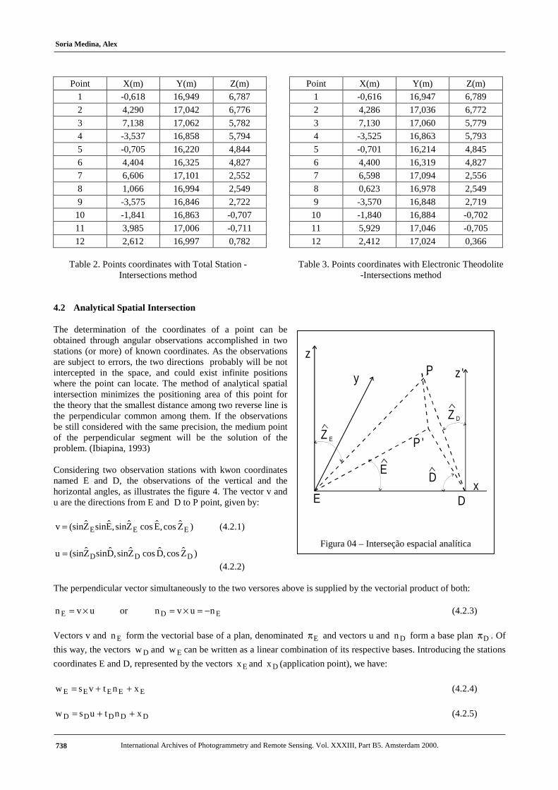
Figura 04 – Interseção espacial analítica

Point X(m) Y(m) Z(m)

1 -0,618 16,949 6,787

2 4,290 17,042 6,776

3 7,138 17,062 5,782

4 -3,537 16,858 5,794

5 -0,705 16,220 4,844

6 4,404 16,325 4,827

7 6,606 17,101 2,552

8 1,066 16,994 2,549

9 -3,575 16,846 2,722

10 -1,841 16,863 -0,707

11 3,985 17,006 -0,711

12 2,612 16,997 0,782

Table 2. Points coordinates with Total Station -Intersections method


1 -0,616 16,947 6,789

2 4,286 17,036 6,772

3 7,130 17,060 5,779

4 -3,525 16,863 5,793

5 -0,701 16,214 4,845

6 4,400 16,319 4,827

7 6,598 17,094 2,556

8 0,623 16,978 2,549

9 -3,570 16,848 2,719

10 -1,840 16,884 -0,702

11 5,929 17,046 -0,705

12 2,412 17,024 0,366

Table 3. Points coordinates with Electronic Theodolite -Intersections method

4.2 Analytical Spatial Intersection

The determination of the coordinates of a point can be obtained through angular observations accomplished in two stations (or more) of known coordinates. As the observations are subject to errors, the two directions probably will be not intercepted in the space, and could exist infinite positions where the point can locate. The method of analytical spatial intersection minimizes the positioning area of this point for the theory that the smallest distance among two reverse line is the perpendicular common among them. If the observations be still considered with the same precision, the medium point of the perpendicular segment will be the solution of the problem. (Ibiapina, 1993) Considering two observation stations with kwon coordinates named E and D, the observations of the vertical and the horizontal angles, as illustrates the figure 4. The vector v and u are the directions from E and D to P point, given by:

)Zcos,EcosZsin,EsinZsin(v EEE= (4.2.1)

)Zcos,DcosZsin,DsinZsin(u DDD=

(4.2.2) The perpendicular vector simultaneously to the two versores above is supplied by the vectorial product of both:

uvn E ×= or ED nuvn −=×= (4.2.3)

Vectors v and En form the vectorial base of a plan, denominated Eπ and vectors u and Dn form a base plan Dπ . Of

this way, the vectors Dw and Ew can be written as a linear combination of its respective bases. Introducing the stations

coordinates E and D, represented by the vectors Ex and Dx (application point), we have:

EEEEE xntvsw ++= (4.2.4)

DDDDD xntusw ++= (4.2.5)

Soria Medina, Alex


being Es and Et the vector base parameters of the plan Eπ . Ds and Dt are the vector base parameters of the plan

Dπ .

The vectors which possess the same direction of the versores v and u, with application points in E and D, are respectively given for:

EEE xvr +λ= (4.2.6)

DDD xur +λ= (4.2.7)

The point P (see figure 4) is calculated by the intersection of the line (defined by the vector in 4.2.6) with the plan (defined in 4.2.5). Therefore, in the intersection, we have:

DDDDDEEE wxntusxvr =++=+λ= (4.2.8)

that rearranging gives:

DEDDDE xxntusv −=++λ (4.2.9)

The equations system above is constituted by three equations and three unknown variables and like vectorial v, u and

Dn are linearly independent, the system admits only a solution. Substituting those values in the equation (4.2.4) or in

the equation (4.2.5) we obtain the coordinates of the point P. In a way similar can calculate the coordinates of PD, equaling rD = wE solving a new system of linear equations, with three equations by three unknown variables. The found values are substituted in the equation (4.2.4) or in the (4.2.7), supplying the coordinates of the point P. The coordinates of the point P is obtained finally of the average between the coordinates of PE and PD, that is:

2

PPP DE +

= (4.2.10)

The next tables (table 4 and table 5) shows the found coordinates for the control points, for the observations with the total station and with the theodolite, respectively.

Point X (m) Y (m) Z (m)

1 -0,618 16,959 6,812

2 4,301 17,111 6,824

3 7,152 17,114 5,820

4 -3,546 16,875 5,821

5 -0,709 16,230 4,868

6 4,327 16,062 4,770

7 6,573 17,032 2,562

8 1,063 16,997 2,570

9 -3,573 16,842 2,743

10 -1,835 16,850 -0,685

11 3,979 16,999 -0,690

12 2,609 16,997 0,803

Table 4. Points coordinates with Total Station –Analytical Spatial Intersection

Point X (m) Y (m) Z (m)

1 -0,616 16,950 6,790

2 4,286 17,039 6,773

3 7,130 17,062 5,780

4 -3,525 16,866 5,794

5 -0,701 16,216 4,846

6 4,400 16,322 4,828

7 6,598 17,097 2,557

8 0,624 16,980 2,549

9 -3,570 16,850 2,719

10 -1,840 16,886 -0,701

11 5,930 17,048 -0,704

12 2,412 17,027 0,366 Table 5. Points coordinates with Electronic Theodolite

– Analytical Spatial Intersection

Soria Medina, Alex


4.3 LEAST SQUARES

To apply the Least Squares method in the adjustment is necessary to establish the mathematical model to be used. In this work each observation can be explicit as a function of unknown parameters, characterizing the parametric method of adjustment (Gemael, 1994). For each observed point it is possible to form two observation equations: one for the horizontal angles and another for the vertical angles. If of the two different stations (E and D) observations, can be accomplished to a same point P and also if these two stations can be considered fixed, we will have 4 equations for 3 unknown. Can be applied the LSM to supply the solution. In the case of three observation stations we will have 6 equations for 3 unknown variables. The observations adjustment has as objective, besides the estimate of only one value for the unknown of the problem, to estimate the precision of this unknown, and an eventual correlation among them. In the coordinates adjustment was obtained quadratic medium errors of the order of 1.8 mm, for the observations with the electronic theodolite, starting from two observation stations (E and D); 1.9 mm for the observations with the total station starting from the same observation stations and a errors of 1.5 mm for the observations with the total station, starting from the three observation stations (E, D and C). In the tables 6 and 7 the adjusted coordinates are shown, having as observations base the stations E and D, from the total station and the theodolite, respectively. The table 8 shows the adjusted coordinates for the accomplish observations with the total station for the base of three points (E, D and C).


1 -0,618 16,950 6,787

2 4,290 17,043 6,776

3 7,138 17,062 5,782

4 -3,538 16,862 5,794

5 -0,705 16,221 4,845

6 4,404 16,325 4,827

7 6,606 17,102 2,552

8 1,066 16,997 2,549

9 -3,575 16,848 2,723

10 -1,842 16,865 -0,707

11 3,985 17,006 -0,711

12 2,612 16,998 0,782 Table 6. Points coordinates with Total Station – Least

Squares


1 -0,616 16,948 6,789

2 4,286 17,037 6,773

3 7,130 17,061 5,781

4 -3,527 16,867 5,793

5 -0,701 16,214 4,845

6 4,400 16,320 4,827

7 6,598 17,095 2,556

8 0,623 16,980 2,550

9 -3,570 16,849 2,716

10 -1,840 16,885 -0,701

11 5,929 17,046 -0,704

12 2,412 17,025 0,362 Table 7. Points coordinates with Electronic Theodolite

– Least Squares


1 -0.619 16.976 6.795

2 4.292 17.054 6.778

3 7.141 17.076 5.784

4 -3.543 16.890 5.803

5 -0.705 16.241 4.849

6 4.405 16.332 4.828

7 6.607 17.106 2.551

8 1.068 17.006 2.549

9 -3.580 16.877 2.727

10 -1.842 16.892 -0.708

11 3.986 17.004 -0.712

12 2.615 16.998 0.781

Table 8 - Points coordinates with Total station for E, D and C base - Least Squares

Soria Medina, Alex


5 CONCLUSIONS

With relationship to the equipment used for the angular information obtaining, to points without target, there is not difference in the coordinates calculated. The observations with electronic theodolite had the same result found in the observations with the total station. For the observation stations number is important to accomplish tests with other base configurations. For the work, three stations were used forming a triangular base, that provided results different from the found to base formed for two stations, besides a larger standard deviation. In relation to the three methods used in the coordinates calculation, everybody presented implement easy with satisfactory results, even so LSM just offers besides the points coordinates, its respective precision.

REFERENCES

Blachut, T. J, Chrzanowski, A., Saastamoinen, J. K., 1979. Urban Surveying and mapping. Springer-Verlag, New York, pp. 162-174. Gemael, C., 1994. Introdução ao ajustamento de observações. Editora da UFPR, Curitiba. Ibiapina, D. S., Silva, I., Manzole Neto, O., 1993. Método topográfico para o posicionamento tridimensional de um ponto. In: Anais do XVI Congresso Brasileiro de Cartografia, Rio de Janeiro, Brasil, pp. 261-267. Richie, W., Wood, M, Wright, R, Tait, D., 1988. Surveying and mapping for fields scientists. Logman Scientific & Technical, New York.

Soria Medina, Alex


topographic survey of the control points for ... · topographic survey of the control points for...

Documents