topographic change detection using cloudcompare … · topographic change detection using...

Topographic Change Detection Using CloudCompare (v1.0)

November, 2013 Page. 1

Topographic Change Detection Using CloudCompare Version 1.0

November, 2013

Emily Kleber, Arizona State University Edwin Nissen, Colorado School of Mines

J Ramón Arrowsmith, Arizona State University Introduction CloudCompare is a powerful piece of open-source point cloud processing software that was developed for civil engineering and manufacturing quality control purposes. It is an open source 3D point cloud and mesh processing software project. It is most powerful in processing and comparing dense point cloud data, visualizing data and data analysis. Some of the data processing capabilities of CloudCompare:

• Projections • Point registration (ICP) • Distance computation (cloud-cloud or cloud-mesh, nearest neighbor distance) • Statistics computation (spatial chi-squared test) • Segmentation (connected components labeling) • Geometric features estimation (density, curvature, roughness, geol. plane orientation)

For more information about CloudCompare and point cloud data: • CloudCompare Website: http://www.danielgm.net/cc/ • CloudCompare Forum: http://www.danielgm.net/cc/forum/ • CloudCompare Wiki: http://www.danielgm.net/cc/doc/wiki/ • ASPRS LAS Specification:

http://www.asprs.org/a/society/committees/standards/LAS_1_4_r13.pdf In this exercise we will use point cloud data from OpenTopography to highlight the features of CloudCompare and do iterative closest point (ICP) analysis on a Aeolian sand dunes. Datasets Used

• Lake Tahoe: http://www.opentopography.org/id/OTLAS.032011.26910.1 • Sand dunes at White Sands National Monument:

o 2009 data: http://www.opentopography.org/id/OTLAS.012013.26913.2 o 2010 data: http://www.opentopography.org/id/OTLAS.022012.26913.1



To introduce manipulating point cloud data in CloudCompare, we will look at classified lidar data and explore how to get from a classified point cloud to a ground model based on discrete ground returns. For this exercise, we will use the Lake Tahoe dataset collected in 2010. First, some general CloudCompare tips:

• Make sure and select the layer in the “DB Tree” window before doing any analysis. • To rename files, select the file and push F2. • To change the background color, Display > Light and Materials > Set Light and

Materials

---- Introduction to CloudCompare with Lake Tahoe Data ---- Load “tahoepoints.las” into CloudCompare by going to File > Open. A window will pop up prompting you to select which field of the LAS header CloudCompare will read. Unless you have specific analyses you’re doing, just select the default (all selected) by clicking ok.

Next a pop-up will come up asking if you’d like to re-center your point cloud. Click yes as this will speed up your processing time.

In the “properties” window, change “Scalar Fields” to “Classification” to show the points by classification. You should see that there are at least two distinguishable classes (unclassified points and ground) for this sample dataset.

In CloudCompare the “scalars” that we will analyze are the actual x,y,z points with attributes attached. Depending on the point cloud data, a range of attributes like classification, intensity, scan angle, return number, ect. will show up. This way to vizualize point cloud data is very useful for understanding your lidar data and understanding what the scalar values mean visually.



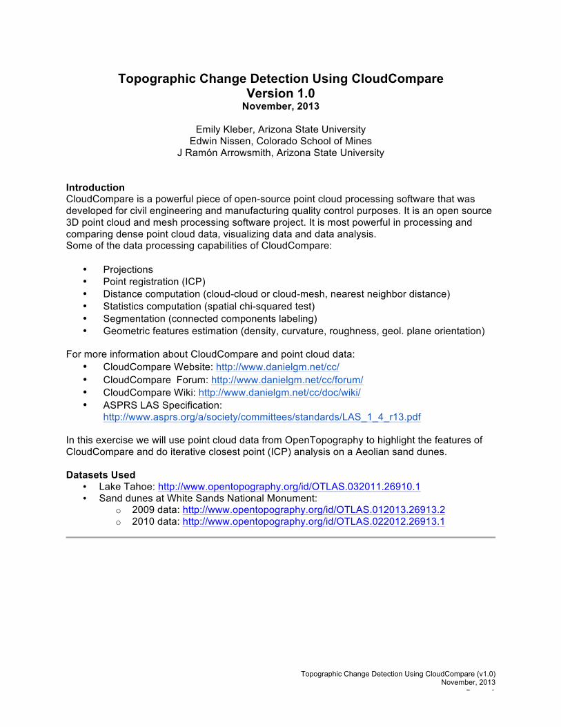
CloudCompare window looking across the surface. Classified ground points are white and unclassified returns are red. You can toggle between color scale of the points in the properties window.

Explore the data by scrolling or using the visualization toolbar on the right. Find a single feature to extract. For this example, we use a tree. Find a view angle that will best capture all the points that define the feature. For this exercise, looking normal to the surface is the best way.

Cutting out a Feature

Select scissors tool from top toolbar. Draw a segment around the feature, making sure to capture all points. Right click to close the polygon. CloudCompare will generate a new layer with the selected feature.



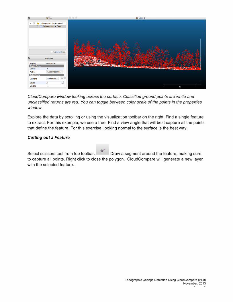
Single tree with classified return number. Blue is first return, green is second and yellow is third.

Building a Ground model

Filter by scalar value: Edit >Scalar Fields > Filter by Value

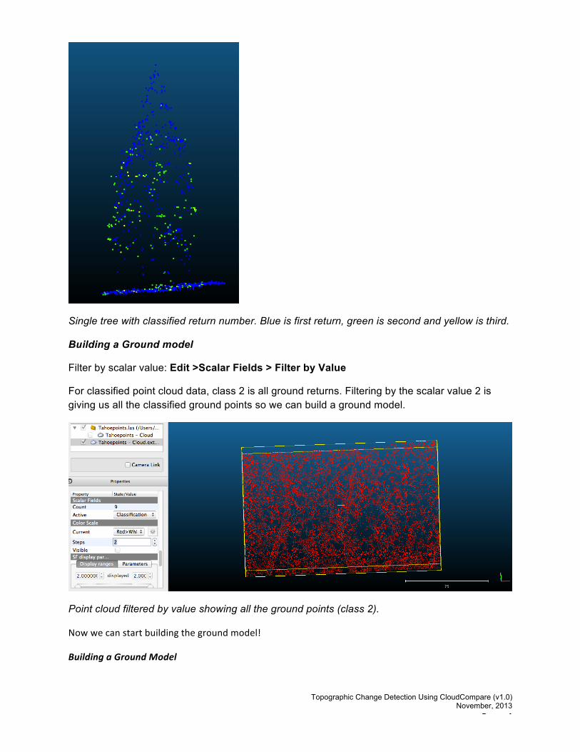
For classified point cloud data, class 2 is all ground returns. Filtering by the scalar value 2 is giving us all the classified ground points so we can build a ground model.

Point cloud filtered by value showing all the ground points (class 2).

Now we can start building the ground model!

Building a Ground Model



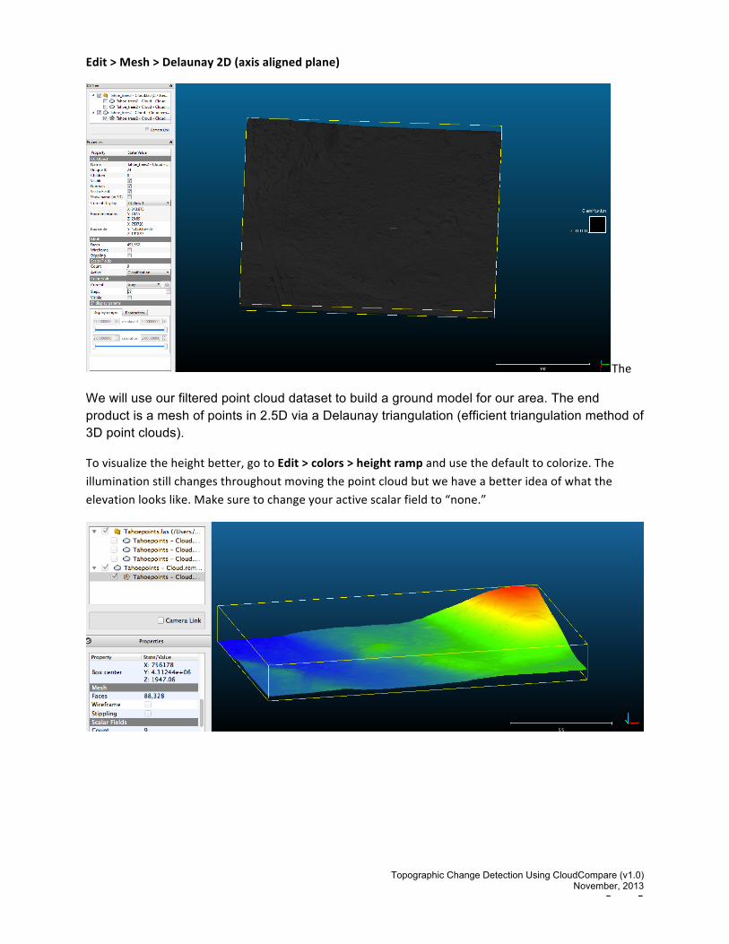
Edit > Mesh > Delaunay 2D (axis aligned plane)

The

We will use our filtered point cloud dataset to build a ground model for our area. The end product is a mesh of points in 2.5D via a Delaunay triangulation (efficient triangulation method of 3D point clouds).

To visualize the height better, go to Edit > colors > height ramp and use the default to colorize. The illumination still changes throughout moving the point cloud but we have a better idea of what the elevation looks like. Make sure to change your active scalar field to “none.”



Isolate Trees

Now we will take a look at the distance between our original point cloud and the mesh we just build. Select the ground model and the full point cloud then go to Tools > Distance > Cloud/Mesh Distance making sure both your mesh and the points are selected.

This tool calculates the distance between the ground surface mesh and the vegetation points. In the console, you will see the statistics calculated from the point cloud.

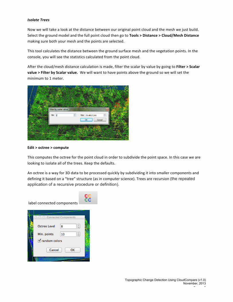
After the cloud/mesh distance calculation is made, filter the scalar by value by going to Filter > Scalar value > Filter by Scalar value. We will want to have points above the ground so we will set the minimum to 1 meter.

Edit > octree > compute

This computes the octree for the point cloud in order to subdivide the point space. In this case we are looking to isolate all of the trees. Keep the defaults.

An octree is a way for 3D data to be processed quickly by subdividing it into smaller components and defining it based on a “tree” structure (as in computer science). Trees are recursion (the repeated application of a recursive procedure or definition).

label connected components



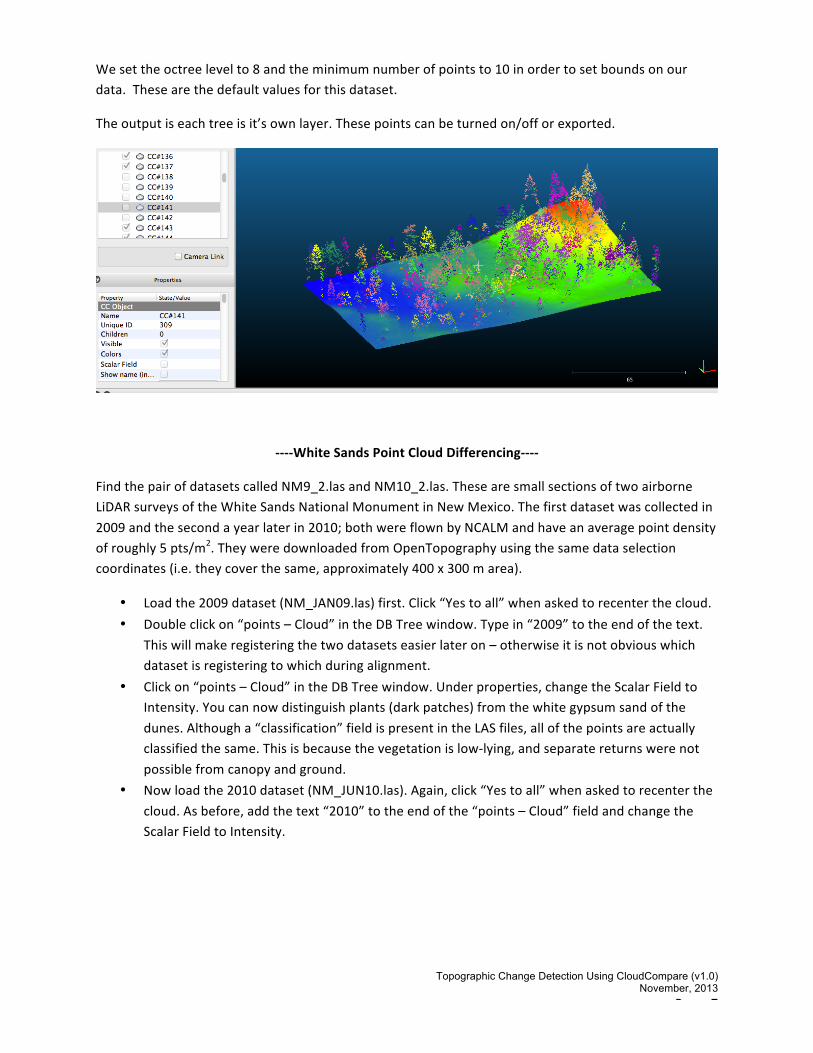
We set the octree level to 8 and the minimum number of points to 10 in order to set bounds on our data. These are the default values for this dataset.

The output is each tree is it’s own layer. These points can be turned on/off or exported.

-‐-‐-‐-‐White Sands Point Cloud Differencing-‐-‐-‐-‐

Find the pair of datasets called NM9_2.las and NM10_2.las. These are small sections of two airborne LiDAR surveys of the White Sands National Monument in New Mexico. The first dataset was collected in 2009 and the second a year later in 2010; both were flown by NCALM and have an average point density of roughly 5 pts/m2. They were downloaded from OpenTopography using the same data selection coordinates (i.e. they cover the same, approximately 400 x 300 m area).

• Load the 2009 dataset (NM_JAN09.las) first. Click “Yes to all” when asked to recenter the cloud. • Double click on “points – Cloud” in the DB Tree window. Type in “2009” to the end of the text.

This will make registering the two datasets easier later on – otherwise it is not obvious which dataset is registering to which during alignment.

• Click on “points – Cloud” in the DB Tree window. Under properties, change the Scalar Field to Intensity. You can now distinguish plants (dark patches) from the white gypsum sand of the dunes. Although a “classification” field is present in the LAS files, all of the points are actually classified the same. This is because the vegetation is low-‐lying, and separate returns were not possible from canopy and ground.

• Now load the 2010 dataset (NM_JUN10.las). Again, click “Yes to all” when asked to recenter the cloud. As before, add the text “2010” to the end of the “points – Cloud” field and change the Scalar Field to Intensity.



1. ALIGNING THE DATASETS

You will see that the two datasets are not aligned. This is because CloudCompare chose different x, y and z shifts for its recentering. There are two ways to fix this. Both involve an initial rough registration (alignment) of the datasets, followed by a fine registration that makes use of the Iterative Closest Point (ICP) algorithm. (ICP will not work if the datasets are not roughly aligned to start with).

1a. Alignment using translate/rotate

We will register the 2010 dataset to the 2009 dataset. The first option for the initial rough alignment to use the Translate/Rotate toolbar option, which looks like this:

• Click on the 2010 points – Cloud dataset in the DB Tree window. Then click on the Translate/Rotate button.

• Right clicking and holding on the 2010 dataset allows you to drag it around the screen. This is a translation.

• Left clicking and holding allows you to rotate the dataset. • A small box should appear on the right of screen.



By checking or unchecking Tx, Ty and Tz, and choosing the correct rotation from the drop down menu, allows you to play with each translational and rotational component at a time.

• To accept the changes to the position of the 2010 dataset, you would click the “tick” mark. However, we will instead click on the “cross” so that we can try the other method of roughly aligning the datasets.

1b. Alignment with equivalent point pairs

The second option for the initial rough registration is to align the datasets by picking (at least three) equivalent point pairs. The toolbar option looks like this:

• Click on “points – Cloud 2009” and control click “points – Cloud 2010” in the DB Tree window so that both are selected. Then click on the button above.

• You are asked to choose which dataset is to be aligned and which is the reference dataset. In this case it doesn’t really matter, but for the time being click “swap” and “OK” so that the 2009 dataset is the reference. A new dialogue will appear in the window

Initially, both datasets are displayed. You can toggle between the datasets by checking and unchecking the “show aligned cloud” and “show registered cloud” boxes in the dialogue.

Next, we need to find features within the two datasets that we can identify as being the same. There are several large, dark bushes that are clear in both datasets which are good features to use. We need to pick out at least three of these – preferably not too close together and not arranged in a straight line – and to select them in both registered and aligned clouds.

• Uncheck “show aligned cloud” so that only the reference cloud is shown.



• Left click on three conspicuous plants which you have identified in both datasets. They are labeled in the order that you click them (R0, R1 and R2), and you should remember this order. I chose these ones:

• Next, uncheck “show reference cloud” and check “show aligned cloud”. Find the same three points in the aligned cloud and click on them, in the same order as you did before. These points will be labeled A0, A1 and A2.

• Finally, click the “align” button. The 2010 dataset should move over the 2009 one. Click on the green “tick” if the results look good.

• A box will appear with the transformation matrix that was applied to the 2010 point cloud. Click “OK”.

1a. Fine registration using ICP

So far we have roughly aligned the two datasets. A final adjustment to this alignment can now be made with ICP. This algorithm relies on two assumptions. (1) Both clouds must already be roughly registered (as we have done). (2) Both clouds should have a reasonably large overlapping surface: ICP will not work in aligning small, overlapping corners of two largely non-‐overlapping datasets. ICP is selected using this toolbar option:

• Click on “points – Cloud 2009” and control click “points – Cloud 2010” in the DB Tree window so that both are selected. Then click on the button above.

• Again, you are asked to choose which dataset is to be aligned (the “Model”) and which is the reference dataset (“Data”). Click “swap” so that the 2009 dataset is the reference.



• The “Error difference” is the minimum registration error decrease between two steps. If the registration error doesn't decrease by more than this quantity between two iterations, then the algorithm will stop. So the smaller this value, the longer it will take to converge, but the finer the result should be.

• The “Random sampling limit” can be lowered to increase computation speed on big clouds. It is an optimization scheme which randomly sub-‐samples the data cloud at each iteration. The higher the number, the larger the sub-‐sampled clouds and the slower the iterations will be.

• For these datasets, there is no need to change the default values for either of these options, so click “OK”.

You should find that the two datasets are now very closely aligned. The reference 2009 dataset has been relabeled “points – Cloud 2009.registered”.

2. IMAGING SAND DUNE MIGRATION WITH POINT DISTANCES

Next, we will look for differences between the 2009 and 2010 datasets.

2a. Cloud to Cloud distances

This function allows you to compute the distances between each point in the reference dataset and each of their closest points in the “compared” dataset. Once the datasets are aligned, this is a powerful way of identifying areas of topographic change.

• Click on “points – Cloud 2009.registered” and control click “points – Cloud 2010” in the DB Tree window so that both are selected. Then click on the button above.

• Make sure the 2009 dataset is the reference (click “swap” if necessary). In this case, it doesn’t really matter which dataset is the reference. However, for pairs of clouds with different extents this does matter. In these instances, you should make sure that the reference cloud extents are wider than the compared cloud ones. This avoids high closest point distances along the boundaries of the smaller dataset.

• The following dialogue box appears.



The default way to compute distances between two point clouds is the “nearest neighbor distance”. This works well if the reference dataset is dense. For sparse reference datasets, you can create a local surface model for each patch of the sparse reference cloud and compute distances to this surface, instead. Options for local surface modeling are shown in the “Local modeling” tab. These datasets are dense enough that you can keep the local model set to “NONE”.

You also have the option of splitting the computed distances into their x, y and z components, by checking the “split X, Y and Z components” box. CloudCompare will generate 3 more scalar fields, one for each axis. Left unchecked, CloudCompare will produce one more scalar field containing only the total distance.

• Click on the “Compute” button.

The compared 2010 dataset is now colored according to a new Scalar Field, called “C2C absolute distances”. Note that the 2009 dataset does not have this new Scalar Field – this is because it was the reference dataset, not the compared one. It is still colored in gray according to the “Intensity” scalar field.



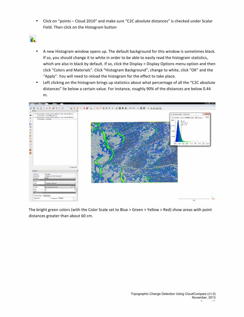
• Click on “points – Cloud 2010” and make sure “C2C absolute distances” is checked under Scalar Field. Then click on the Histogram button

• A new Histogram window opens up. The default background for this window is sometimes black. If so, you should change it to white in order to be able to easily read the histogram statistics, which are also in black by default. If so, click the Display > Display Options menu option and then click “Colors and Materials”. Click “Histogram Background”, change to white, click “OK” and the “Apply”. You will need to reload the histogram for the effect to take place.

• Left clicking on the histogram brings up statistics about what percentage of all the “C2C absolute distances” lie below a certain value. For instance, roughly 90% of the distances are below 0.44 m.

The bright green colors (with the Color Scale set to Blue > Green > Yellow > Red) show areas with point distances greater than about 60 cm.

topographic change detection using cloudcompare … · topographic change detection using...

Documents