meaningful change detection and sediment...
TRANSCRIPT

Meaningful Change Detection and Sediment Budgeting from Repeat Topographic Data
NSF LiDaR Tools Workshop – Session 2B
June 1, 2010 Boulder, Colorado
Instructor: Joe Wheaton
Introduction As repeat topographic data sets become an increasingly popular form of scientific monitoring, the need grows for robust methods of quantifying and accounting for uncertainties in those data to reliably distinguish between calculated changes likely to be real versus those changes one cannot distinguish from noise. Once the uncertainties in repeat topographic data sets are accounted for, the more interesting question of how to interpret the data and use it to test specific hypotheses remains. In this session, participants will learn how to use the DEM of Difference Uncertainty Analysis Software to do both an uncertainty analysis of repeat topographic datasets and interpret the data in terms of sediment budgets.
For More Information (including references & publications): http://www.joewheaton.org/Home/research/projects-1/morphological-sediment-budgeting
Download software at: http://www.joewheaton.org/Home/research/software/dod-uncertainty-analysis-software
Chapter Contents This PDF includes the workshop presentation as well workshop exercises, and documentation for DoD 3.0 Beta. Use the bookmarks in the PDF version to help you navigate.

Workshop Session 2B - DoD Analysis
1
Meaningful Change Detection and Sediment Budgeting from Repeat Topographic DataRepeat Topographic Data
NSF WORKSHOP – Session 2BNew Tools in Process-Based Analysis of LiDaR Topographic DataJune 1, 2010
Joe Wheaton
ACKNOWLEDGEMENTS
Matlab Software & Methods presented developed in association with:
• James Brasington
• Steve Darby & David Sear
ArcGIS Software developed with:
• Chris Garrard
Funding from:
Workshop Session 2B - DoD Analysis
2
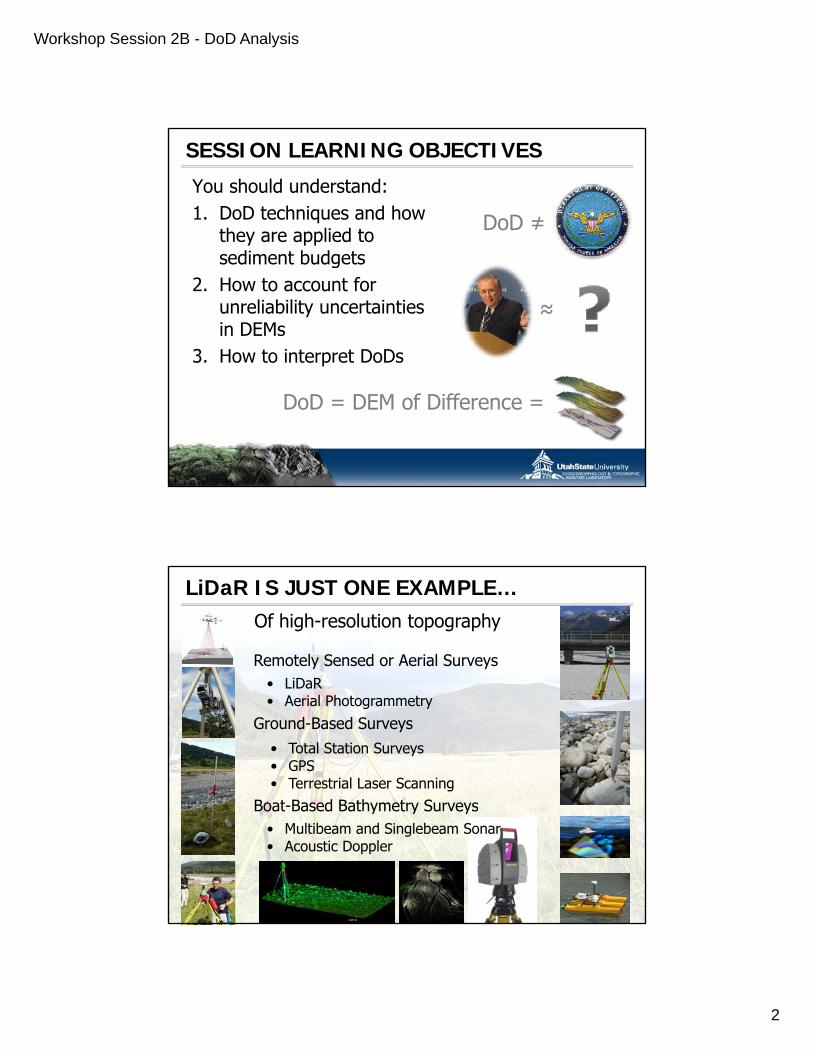
SESSION LEARNING OBJECTIVES
You should understand:1. DoD techniques and how
they are applied to DoD ≠
sediment budgets2. How to account for
unreliability uncertainties in DEMs
3. How to interpret DoDs
≈
DoD = DEM of Difference =
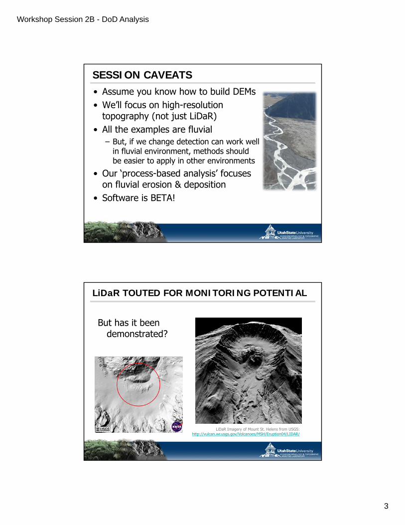
LiDaR IS JUST ONE EXAMPLE…
• LiDaRRemotely Sensed or Aerial Surveys
Of high-resolution topography
• LiDaR• Aerial Photogrammetry
• Total Station Surveys• GPS• Terrestrial Laser Scanning
Ground-Based Surveys
Boat Based Bathymetry Surveys• Multibeam and Singlebeam Sonar• Acoustic Doppler
Boat-Based Bathymetry Surveys
Workshop Session 2B - DoD Analysis
3
SESSION CAVEATS• Assume you know how to build DEMs• We’ll focus on high-resolution
topography (not just LiDaR)• All the examples are fluvial
– But, if we change detection can work well in fluvial environment, methods should be easier to apply in other environments
• Our ‘process-based analysis’ focuses on fluvial erosion & depositionon fluvial erosion & deposition
• Software is BETA!
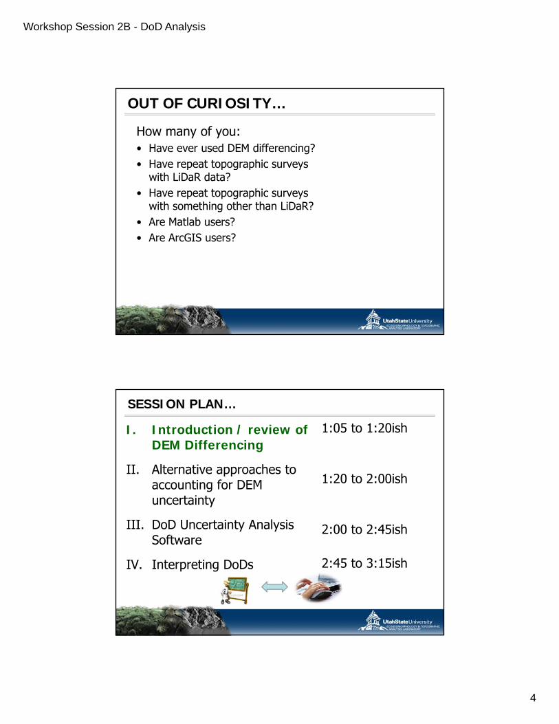
LiDaR TOUTED FOR MONITORING POTENTIAL
But has it been demonstrated?
LiDaR Imagery of Mount St. Helens from USGS: http://vulcan.wr.usgs.gov/Volcanoes/MSH/Eruption04/LIDAR/
Workshop Session 2B - DoD Analysis
4
OUT OF CURIOSITY…
How many of you:• Have ever used DEM differencing?• Have repeat topographic surveys
with LiDaR data?• Have repeat topographic surveys
with something other than LiDaR?• Are Matlab users?• Are ArcGIS users?
SESSION PLAN…
I. Introduction / review of DEM Differencing
II Alternative approaches to
1:05 to 1:20ish
II. Alternative approaches to accounting for DEM uncertainty
III. DoD Uncertainty Analysis Software
1:20 to 2:00ish
2:00 to 2:45ish
IV. Interpreting DoDs 2:45 to 3:15ish

Workshop Session 2B - DoD Analysis
5
SESSION DETAIL PLAN – I.
I. Introduction / review of DEM DifferencingA. Background on monitoring with
repeat topographic surveying for di b d isediment budgeting
B. Basic DEM DifferencingC. Raster Calculator DoD ExampleD. Questions
THE BACKGROUND PROBLEM
• Rivers change through time… how do we detect that change?

Workshop Session 2B - DoD Analysis
6
BECOMING EASIER TO TRACK CHANGE...
© Wheaton (2008)
HOW CAN WE CALCULATE CHANGE?
• Given these DEMs through time, what could we use to calculate change?

Workshop Session 2B - DoD Analysis
7
SESSION DETAIL PLAN – I.
I. Introduction / review of DEM DifferencingA. Background on monitoring with repeat
topographic surveying for sediment b dbudgeting
B. Basic DEM DifferencingC. Raster Calculator DoD ExampleD. Questions
DEM DIFFERENCINGSimple method of quantifying spatial
variations in change in storage terms of a sediment budget.
RASTER CALCULATOR….
CONSERVATION OF MASS VOLUMETRIC
© Wheaton (2008)Mclean & Church (1988) – Water Resources Research
dt
dVQQ b
bobi )1( Porosity of bed material
Volumetric rate of bed material transport
Workshop Session 2B - DoD Analysis
8
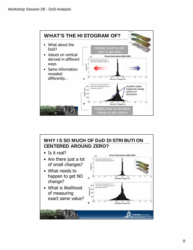
WHAT’S THE HISTOGRAM OF?
• What about the DoD?
• Values on vertical derived in different
Multiply count by cell size2 to get area
derived in different ways
• Same information revealed differently…
ErosionErosion DepositionDeposition
Amplifies higher
Multiply area by elevation change to get volume
p gmagnitude changeportions of distribution
WHY IS SO MUCH OF DoD DISTRIBUTION CENTERED AROUND ZERO?• Is it real?• Are there just a lot
fof small changes?• What needs to
happen to get NO change?
• What is likelihood of measuring exact same value?

Workshop Session 2B - DoD Analysis
9
SESSION DETAIL PLAN – I.
I. Introduction / review of DEM DifferencingA. Background on monitoring with repeat
topographic surveying for sediment b dbudgeting
B. Basic DEM DifferencingC. Raster Calculator DoD ExampleD. Questions
DEM DIFFERENCINGSimple method of quantifying spatial
variations in change in storage terms of a sediment budget.
RASTER CALCULATOR….
CONSERVATION OF MASS VOLUMETRIC
© Wheaton 2008Mclean & Church (1988) – Water Resources Research
dt
dVQQ b
bobi )1( Porosity of bed material
Volumetric rate of bed material transport
Workshop Exercise I - Raster Calculator DoD Example
1 of 3
Using ArcGIS’s Raster Calculator (Spatial Analyst) to Calculate DoD
Produced by Joe Wheaton Updated: May 20, 2010
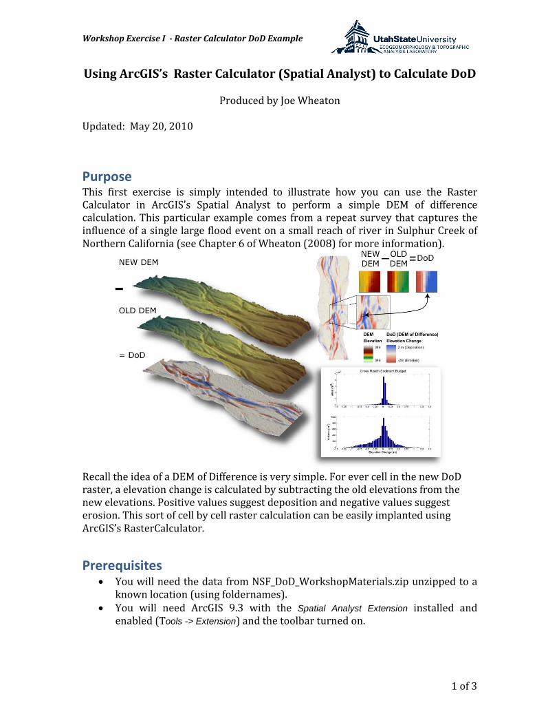
Purpose This first exercise is simply intended to illustrate how you can use the Raster Calculator in ArcGIS’s Spatial Analyst to perform a simple DEM of difference calculation. This particular example comes from a repeat survey that captures the influence of a single large flood event on a small reach of river in Sulphur Creek of Northern California (see Chapter 6 of Wheaton (2008) for more information).
Recall the idea of a DEM of Difference is very simple. For ever cell in the new DoD raster, a elevation change is calculated by subtracting the old elevations from the new elevations. Positive values suggest deposition and negative values suggest erosion. This sort of cell by cell raster calculation can be easily implanted using ArcGIS’s RasterCalculator.
Prerequisites • You will need the data from NSF_DoD_WorkshopMaterials.zip unzipped to a
known location (using foldernames). • You will need ArcGIS 9.3 with the Spatial Analyst Extension installed and
enabled (Tools -> Extension) and the toolbar turned on.

Workshop Exercise I - Raster Calculator DoD Example
2 of 3
Procedure 1. Open a blank new Map Document in ArcGIS 2. Use the Add Data command to add the older DEM first by navigating to the
*/NSF_LiDaR_2010\NSF_DoD_WorkshopMaterials\ArcMap\Data\2005Dec folder and add the 2005 Topo.lyr. This loads both the DEM and hillshade in a group.
3. Next, use the Add Data command to add the newer DEM first by navigating to */NSF_LiDaR_2010\NSF_DoD_WorkshopMaterials\ArcMap\Data\2006Feb folder and add the 2006 Topo.lyr. Notice the differences between the two layers (you can use the Effects toolbar and the Swipe Layer command to view the differences).
4. Using the Spatial Analyst toolbar, go to Spatial Analyst -> Raster Calculator.
Double click on the new DEM first (2006 February DEM) and the hit the minus (-) button, then double click on the old DEM (2005 December DEM) to build an expression in the Rater Calculator dialog. Click Evaluate to see the DEM of Difference (DoD). This will add a layer called Calculation to the Data Frame.
5. To visualize this layer a little better we will import a symbology from a layer file. Right click on the Calculation layer and click on Layer Properties. Under the Symbology tab, change this from a Stretched display to a Classified. If it asks you to Compute Histogram, click Yes. In the upper right corner, click on the Import button:

Workshop Exercise I - Raster Calculator DoD Example
3 of 3
Load the DoD.lyr from the *\NSF_LiDaR_2010\NSF_DoD_WorkshopMaterials\ArcMap\Data\ directory.
6. Next rename the Calculation layer to DoD: 2006-2005 by right clicking on the layer and selecting Rename.
7. Finally, save the DoD by right clicking on the layer and going to Data -> Export…
References
Wheaton JM. 2008. Uncertainty in Morphological Sediment Budgeting of Rivers. Unpublished PhD, University of Southampton, Southampton, 412 pp. Available at: http://www.joewheaton.org/Home/research/projects-1/morphological-sediment-budgeting/phdthesis.

Workshop Session 2B - DoD Analysis
10
SESSION DETAIL PLAN – I.
I. Introduction / review of DEM DifferencingA. Background on monitoring with repeat
topographic surveying for sediment b dbudgeting
B. Basic DEM DifferencingC. Raster Calculator DoD ExampleD. Questions
SESSION PLAN…
I. Introduction / review of DEM Differencing
II Alternative approaches to
1:05 to 1:20ish
II. Alternative approaches to accounting for DEM uncertainty
III. DoD Uncertainty Analysis Software
1:20 to 2:00ish
2:00 to 2:45ish
IV. Interpreting DoDs 2:45 to 3:15ish
Workshop Session 2B - DoD Analysis
11
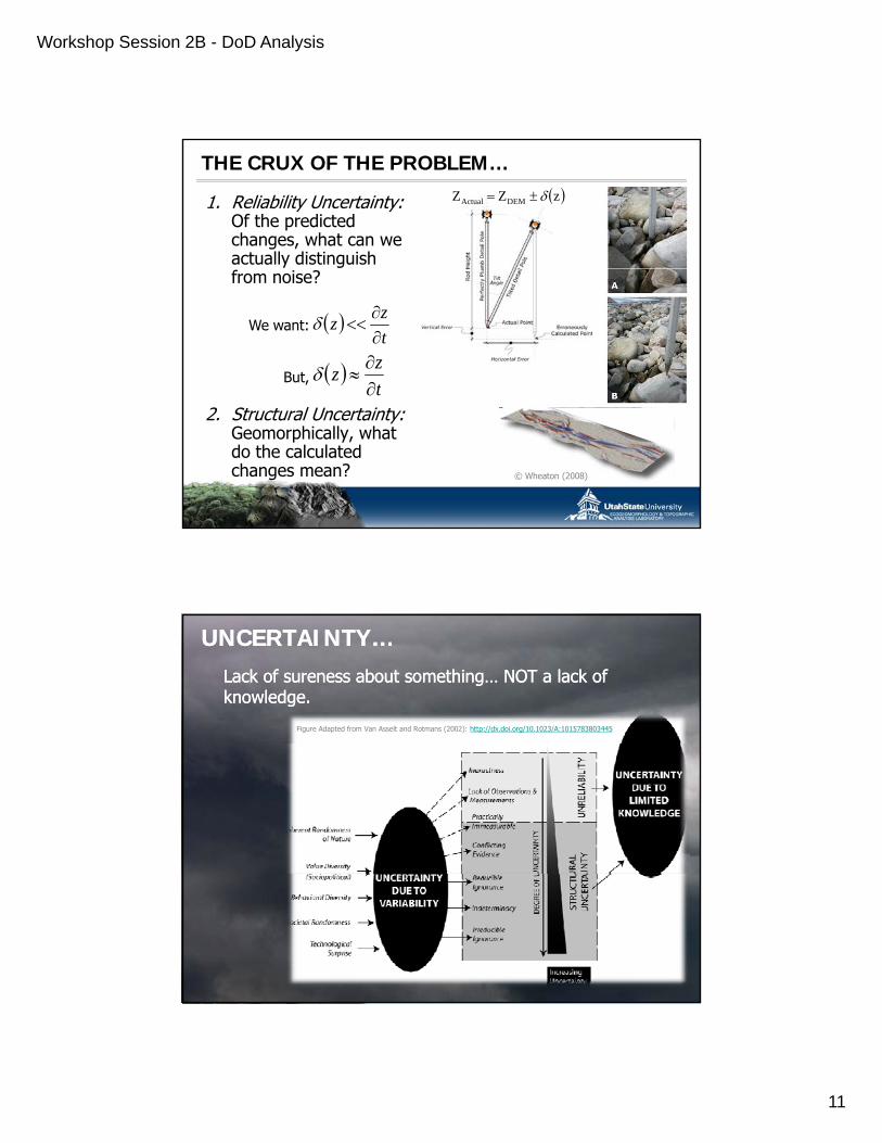
THE CRUX OF THE PROBLEM…
1. Reliability Uncertainty:Of the predicted changes, what can we actually distinguish
z Z Z DEMActual
from noise?
t
zz
t
zz
We want:
But,
2. Structural Uncertainty:Geomorphically, what do the calculated changes mean? © Wheaton (2008)
UNCERTAINTY…UNCERTAINTY…Lack of sureness about something… NOT a lack of Lack of sureness about something… NOT a lack of knowledge.knowledge.
Figure Adapted from Van Asselt and Rotmans (2002): http://dx.doi.org/10.1023/A:1015783803445

Workshop Session 2B - DoD Analysis
12
SESSION DETAIL PLAN – II.
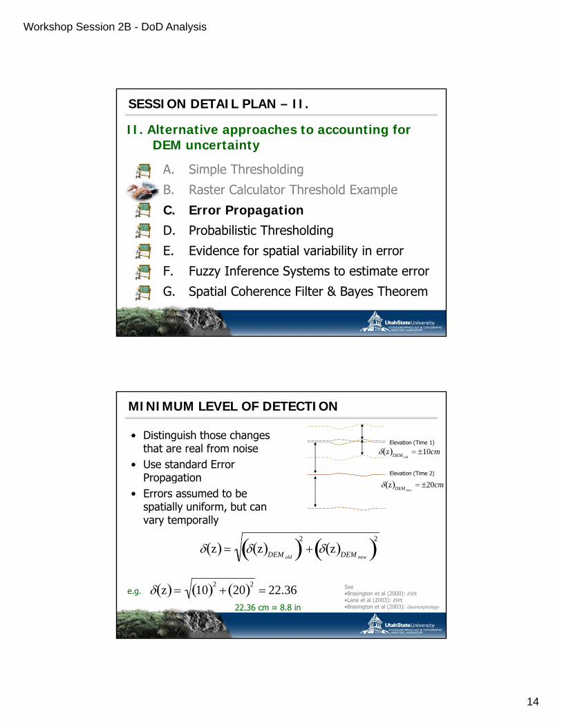
II. Alternative approaches to accounting for DEM uncertainty
A Simple ThresholdingA. Simple ThresholdingB. Raster Calculator Threshold Example
C. Error Propagation
D. Probabilistic Thresholding
E. Evidence for spatial variability in errorE. Evidence for spatial variability in error
F. Fuzzy Inference Systems to estimate error
G. Spatial Coherence Filter & Bayes Theorem
MINIMUM LEVEL OF DETECTION
• Distinguish those changes that are real from noise
• Use standard Error P i
Elevation (Time 1)
Elevation (Time 2)
z DEM old 10cm
Propagation• Errors assumed to be
spatially uniform, but can vary temporally
z z DEM old 2 z DEM new
2
Elevation (Time 2)
z DEM new 20cm
DEM old DEM new
See •Brasington et al (2000): ESPL•Lane et al (2003): ESPL•Brasington et al (2003): Geomorphology
z 10 2 20 2 22.3622.36 cm ≈ 8.8 in
e.g.

Workshop Session 2B - DoD Analysis
13
HOW DOES A MINLoD GET APPLIED?
• You take original DoD, and remove all changes <= minLoDg min
• For example +/- 20 cm
• How would you do that?
• What is the• What is the assumption here?
SESSION DETAIL PLAN – II.
II. Alternative approaches to accounting for DEM uncertainty
A Simple ThresholdingA. Simple Thresholding
B. Raster Calculator Threshold ExampleC. Error Propagation
D. Probabilistic Thresholding
E. Evidence for spatial variability in errorE. Evidence for spatial variability in error
F. Fuzzy Inference Systems to estimate error
G. Spatial Coherence Filter & Bayes Theorem

Workshop Exercise II - Thresholding DoD Example
1 of 3
Using ArcGIS’s Raster Calculator to Threshold a DoD
Produced by Joe Wheaton Updated: May 20, 2010
Purpose After making your own DoD in Exercise I, we would like to apply a typical form of simple uncertainty analysis used in change detection. The idea is to threshold the DoD based on a minimum level of detection (minLoD). As with the example below (at left), your DoD shows some change calculated over the entire raster. The argument is that at below some threshold (20 cm in the example at right below), we cannot distinguish real changes from noise.
Customarily, the changes beneath the minLoD are simply discarded1
Prerequisites
and those above the threshold are assumed to be large enough to be real. See Chapter 4 of Wheaton (2008) or Wheaton et al. (2010) for more information on thresholding.
• You will need your DoD layer from the first exercise. • You will need ArcGIS 9.3 with the Spatial Analyst Extension installed and
enabled (Tools -> Extension) and the toolbar turned on. 1 It should be noted that more sophisticated treatments exist of the data below the threshold (e.g. Lane et al. 2003). Some apply a lesser weight to data below the threshold, others use it as an estimate of +/- error volumes.

Workshop Exercise II - Thresholding DoD Example
2 of 3
Procedure 1. Either use your Map Document from the first exercise or open a blank new
Map Document in ArcGIS. If you are starting over, use the Add Data command to add the DoD you previously created.
2. First we will create a mask of the threshold using simple conditional logic to create a threshold of +/- 10 cm. Using the Spatial Analyst toolbar, go to Spatial Analyst -> Raster Calculator.
Use the expression [DoD] > 0.10 | [DoD] < - 0.10 where [DoD] is whatever layer name your DoD is (recall you can double click on your DoD in the layer list to get it to populate the expression builder). When you click Evaluate, this should return a Calculation raster, which has 0’s everywhere that the expression is false (i.e. when the DoD is below the threshold) and 1’s everywhere the expression is true.
3. Using the Spatial Analyst -> Reclassify command, select the Calculation layer as your Input Raster, and change all the 0s to NoData and keep the 1’s as 1’s:
Use the defaults for therest and Click OK.
4. Using the Spatial Analyst -> Raster Calculator again, multiply your new Reclass of Calculation (mask) layer by your DoD Layer: [Relcass of Calculation]

Workshop Exercise II - Thresholding DoD Example
3 of 3
* [DoD]. This will return a new Calculation2 layer, which represents your thresholded DoD.
5. Turn off the other layers so you can see what has been cut out of this layer. Bring up the Layer Properties for this Calculation2 layer, and go to the Symbology tab. As with the first exercise, change this from a Stretched display to a Classified. If it asks you to Compute Histogram, click Yes. In the upper right corner, again click on the Import button. However, this time you can simply select your DoD layer (presuming it is loaded in the map document instead of loading the DoD.lyr file from the disk.
6. If you want to save this thresholded DoD, Right click on the layer and use
either Data -> Make Permanent or Data -> Export Data…
References Lane SN, Westaway RM and Hicks DM. 2003. Estimation of erosion and deposition
volumes in a large, gravel-bed, braided river using synoptic remote sensing. Earth Surface Processes and Landforms. 28(3): 249-271. DOI: 10.1002/esp.483.
Wheaton JM. 2008. Uncertainty in Morphological Sediment Budgeting of Rivers. Unpublished PhD, University of Southampton, Southampton, 412 pp. Available at: http://www.joewheaton.org/Home/research/projects-1/morphological-sediment-budgeting/phdthesis.
Wheaton JM, Brasington J, Darby SE and Sear D. 2010. Accounting for uncertainty in DEMs from repeat topographic surveys: Improved sediment budgets Earth Surface Processes and Landforms. 35(2): 136-156. DOI: 10.1002/esp.1886.
Workshop Session 2B - DoD Analysis
14
SESSION DETAIL PLAN – II.
II. Alternative approaches to accounting for DEM uncertainty
A Simple ThresholdingA. Simple Thresholding
B. Raster Calculator Threshold Example
C. Error PropagationD. Probabilistic Thresholding
E. Evidence for spatial variability in errorE. Evidence for spatial variability in error
F. Fuzzy Inference Systems to estimate error
G. Spatial Coherence Filter & Bayes Theorem
MINIMUM LEVEL OF DETECTION
• Distinguish those changes that are real from noise
• Use standard Error P i
Elevation (Time 1)
Elevation (Time 2)
z DEM old 10cm
Propagation• Errors assumed to be
spatially uniform, but can vary temporally
z z DEM old 2 z DEM new
2
Elevation (Time 2)
z DEM new 20cm
DEM old DEM new
See •Brasington et al (2000): ESPL•Lane et al (2003): ESPL•Brasington et al (2003): Geomorphology
z 10 2 20 2 22.3622.36 cm ≈ 8.8 in
e.g.

Workshop Session 2B - DoD Analysis
15
WHAT ARE TYPICAL ERRORS?
• LiDaR : +/- 12 to 25 cm• Aerial Photogrammetry : +/- 10 to 15 cm
Remotely Sensed or Aerial Surveys
• Total Station Surveys : +/- 2 to 10 cm
• GPS: : +/- 3 to 12 cm
Ground-Based Surveys
• Terrestrial Laser Scanning: +/-0.5 to 4 cm
SO WHAT WOULD PROPAGATED ERRORS BE?
• LiDaR : +/- 12 to 25 cm (17 to 36 cm minLoD)
• Aerial Photogrammetry : +/- 10 to 15
Remotely Sensed or Aerial Surveys
• Aerial Photogrammetry : +/ 10 to 15 cm(14 to 22 cm minLoD)
• Total Station Surveys : +/- 2 to 10 cm (3 to 14 cm minLoD)
• GPS: : +/- 3 to 12 cm (4 to 17
Ground-Based Surveys
cm minLoD)• Terrestrial Laser Scanning: +/-
0.5 to 4 cm (0.7 to 6 cm minLoD)

Workshop Session 2B - DoD Analysis
16
VARYING minLoD THRESHOLDS
THE PROBLEM: Discards between:
newold DEMDEMf z,zz
22 zzznewold DEMDEM
•70% & 95% of areal budget •45% & 65% of volumetric budget
Much of which is probably meaningful change
© Wheaton 2008
SESSION DETAIL PLAN – II.
II. Alternative approaches to accounting for DEM uncertainty
A Simple ThresholdingA. Simple Thresholding
B. Raster Calculator Threshold Example
C. Error Propagation
D. Probabilistic ThresholdingE. Evidence for spatial variability in errorE. Evidence for spatial variability in error
F. Fuzzy Inference Systems to estimate error
G. Spatial Coherence Filter & Bayes Theorem
Workshop Session 2B - DoD Analysis
17
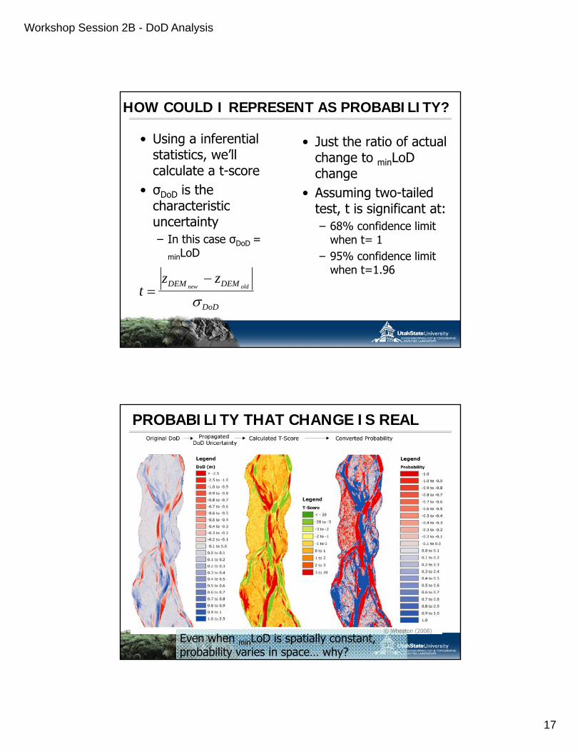
HOW COULD I REPRESENT AS PROBABILITY?
• Using a inferential statistics, we’ll calculate a t-score
• Just the ratio of actual change to minLoD change
• σDoD is the characteristic uncertainty– In this case σDoD =
minLoD
change • Assuming two-tailed
test, t is significant at: – 68% confidence limit
when t= 1– 95% confidence limit
when t=1.96
t zDEM new
zDEM old
DoD
PROBABILITY THAT CHANGE IS REAL
Even when minLoD is spatially constant, probability varies in space… why?
© Wheaton (2008)

Workshop Session 2B - DoD Analysis
18
SESSION DETAIL PLAN – II.
II. Alternative approaches to accounting for DEM uncertainty
A Simple ThresholdingA. Simple Thresholding
B. Raster Calculator Threshold Example
C. Error Propagation
D. Probabilistic Thresholding
E. Evidence for spatial variability in errorE. Evidence for spatial variability in errorF. Fuzzy Inference Systems to estimate error
G. Spatial Coherence Filter & Bayes Theorem
IS UNCERTAINTY SPATIALLY UNIFORM?
• If so what does that imply?• If not what does that imply?

Workshop Session 2B - DoD Analysis
19
TO TEST UNCERTAINTY AS A FUNCTION OF SPACE:
• Conducted some experimentsR (th t h t h d)
z DEM f x,y,.....
• Resurvey same area (that has not changed) over and over and over again, using– Same techniques– Different sampling strategies– Different operators
Different interpolations– Different interpolations
• Use variance of surface representation to test for spatial dependence of error
SOME GAMES

Workshop Session 2B - DoD Analysis
20
EMPIRICAL EVIDENCE OF SPATIAL PATERN
Bootstrapping test….
SESSION DETAIL PLAN – II.
II. Alternative approaches to accounting for DEM uncertaintyA. Simple Thresholding
B. Raster Calculator Threshold Example
C. Error Propagation
D. Probabilistic Thresholding
E. Evidence for spatial variability in error
F. Fuzzy Inference Systems to estimate error
G. Spatial Coherence Filter & Bayes Theorem

Workshop Session 2B - DoD Analysis
21
CRISP VS. FUZZY SETS…
Fuzzy set theory… useful for classifying continuous variables
ARGUMENT FOR FUZZY

Workshop Session 2B - DoD Analysis
22
AN INFERENCE SYSTEM – RULE BASED
STEPS IN A FUZZY INFERENCE SYSTEM
1. Define output categories and membership functions
2 Decide inputs2. Decide inputs1. Define categories and membership functions for
each input
3. Build rule table (weight rules if desired)4. Apply each relevant rule5 Method for combining rules to5. Method for combining rules to 6. Method for defuzzifying output (back to crisp
value)

Workshop Session 2B - DoD Analysis
23
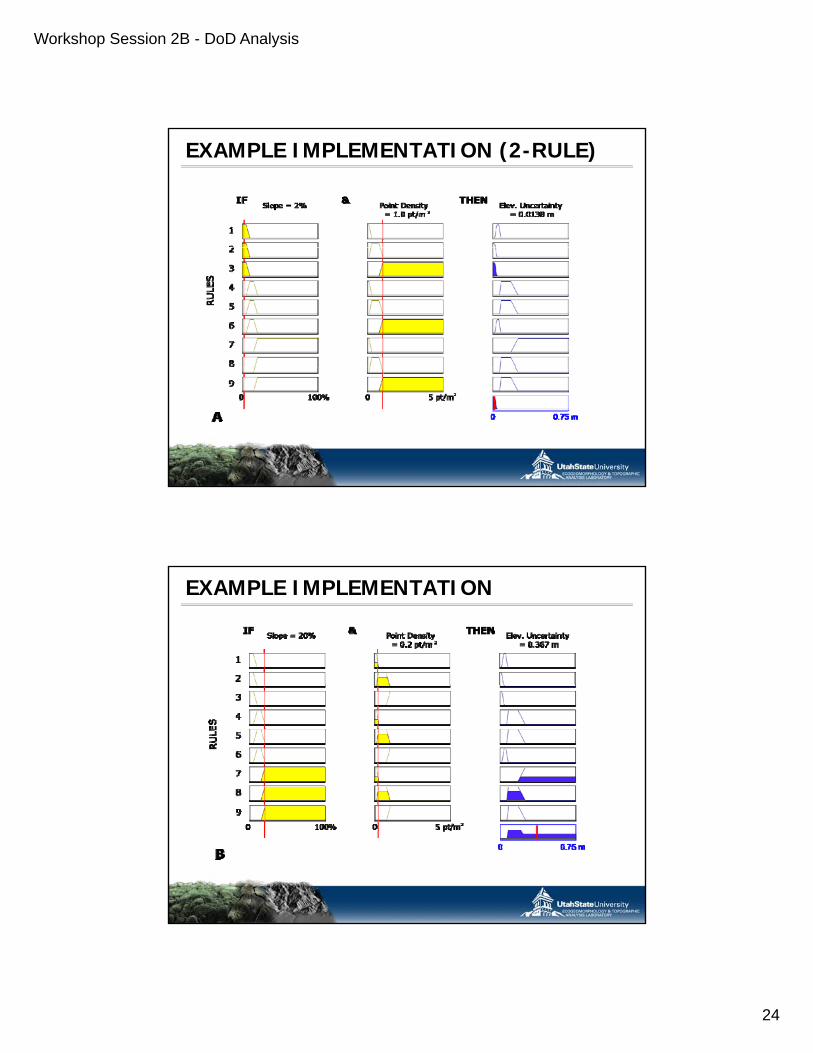
A SIMPLE TWO RULE SYSTEM…
• Given a point cloud• Relationship between
topographic complexity (slope) and sampling (point density)
DEFINING MEMBERSHIP FUNCTIONS
• Define Inputs & Output
• Define number of categories in eachR
yxfDEM ,?,z
• Represent categorical uncertainty (vagueness) with membership functions
• Decide rules…
Workshop Session 2B - DoD Analysis
24
EXAMPLE IMPLEMENTATION (2-RULE)
EXAMPLE IMPLEMENTATION

Workshop Session 2B - DoD Analysis
25
LETS APPLY THIS WITH A REAL EXAMPLE
APPLY FIS ON CELL BY CELL BASIS

Workshop Session 2B - DoD Analysis
26
WHAT DOES FIS DO?
• Recovers some low magnitude change & discards some higher magnitude change
• More realistic bimodal distribution…
Wet
Yea
rea
rD
ry Y
e
Unthresholded Spatailly-UniformminLoD =+/- 10cm
FIS95% C.I.
PROBLEM: THE SMALL STUFF?
• Although calculating a spatially variable minLoD helps, we still never actually include small elevation changes that approach zero
• This is not to say that such changes can’t be real, just that our methods for
i h tmeasuring change can not distinguish these changes from noise

Workshop Session 2B - DoD Analysis
27
SESSION DETAIL PLAN – II.
II. Alternative approaches to accounting for DEM uncertaintyA. Simple Thresholding
B. Raster Calculator Threshold Example
C. Error Propagation
D. Probabilistic Thresholding
E. Evidence for spatial variability in error
F. Fuzzy Inference Systems to estimate error
G. Spatial Coherence Filter & BayesTheorem
SPATIAL COHERENCE OF CHANGE?
• Is change map a checkerboard of blue and red or do changes exhibit coherent spatial patterns?
• PREMISE:– Change is more believable if it is
spatially consistent with its neighbors

Workshop Session 2B - DoD Analysis
28
SPATIAL COHERENCE FILTER
• Normally, if a cell is below minLoD it is discarded
• Let normal minLoD = -5 cmIf hi d i• If everything around me is also erosional, there is a higher likelihood that the small change is real
• By contrast, if everything around me is depositional, th l b bilit th tthen lower probability that change is real
UPDATE USING BAYES THEOREM
p E j A p A EJ p E j p A EJ p E j p A Ei p Ei
• P(Ej|A) is updated (posterior probability)• P(Ej) is initial probability (a priori probability)• P(A|Ej) is conditional probability usingprobability using spatial coherence filter (new information)•Subscript i denotes inverse probability

Workshop Session 2B - DoD Analysis
29
EXAMPLE: WHAT IS P(Ej|A)?
p E j A 0.85 0.68
0.85 0.68 0.15 0.32 0.92
p E j A p A EJ p E j p A EJ p E j p A Ei p Ei
LET:• P(Ej) = 0.68• P(A|Ej) = 0.85• In other words, additional information from spatial coherence index increasedindex increased probability that change is real….
INFLUENCE OF SPATIAL COHERENCE FILTER
• Effectively a better spatial discriminator• For ECD, recovers some low magnitudesome low magnitude changes

Workshop Session 2B - DoD Analysis
30
SO COMBINING FIS & SC FILTER…
• We get a map of probability that change is real
• We choose the confidence interval we want to threshold this at (e.g. 95%, 50%)
• What is more conservative?
• Be careful with systematic yerrors…
SENSITVITY OF THRESHOLD?

Workshop Session 2B - DoD Analysis
31
SESSION PLAN…
I. Introduction / review of DEM Differencing
II Alternative approaches to
1:05 to 1:20ish
II. Alternative approaches to accounting for DEM uncertainty
III. DoD Uncertainty Analysis Software
1:20 to 2:00ish
2:00 to 2:45ish
IV. Interpreting DoDs 2:45 to 3:15ish
SESSION DETAIL PLAN – III.
III. DoD Uncertainty Analysis Software
A Matlab -> DoD 3 0 Wizard ExampleA. Matlab > DoD 3.0 Wizard ExampleB. ArcGIS -> DoD 4.0 BETA Demo
C. Questions and Self-Paced Examples
Workshop Session 2B - DoD Analysis
32
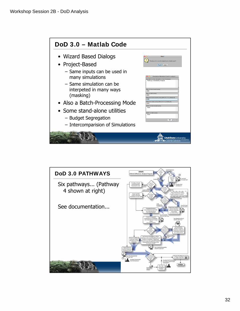
DoD 3.0 – Matlab Code
• Wizard Based Dialogs• Project-Based
– Same inputs can be used inSame inputs can be used in many simulations
– Same simulation can be interpeted in many ways (masking)
• Also a Batch-Processing Moded l l• Some stand-alone utilities
– Budget Segregation– Intercomparision of Simulations
DoD 3.0 PATHWAYS
Six pathways... (Pathway 4 shown at right)
See documentation...

DoD3 Uncertainty Analysis Software Tutorial
1 of 44
DoD 3.0 Beta Tutorial DEM of Difference Uncertainty Analysis Software
Produced by Joe Wheaton Copyright (C) 2009 Wheaton Updated: November 1, 2009
Introduction This tutorial is intended to help you through the different pathways you can take through the DoD3 software wizard. The tutorial will use the example data from Sulphur Creek provided with the zip file. The first part covers basics of navigating through the software. The later half covers more advanced topics for when you start preparing your own data for use in the software or modifying the source code yourself. The screen shots in this tutorial were taken from a Mac OS, and the appearance will be slightly different in Windows. The tutorial is not comprehensive, but should hopefully give you enough direction to navigate through the program. If you experience crashes during the program, check the Matlab Scripts and Functions section and confirm that you have met the minimum requirements specified in the ReadMe file. You may need to make minor tweaks to the code to get it to work for your circumstances. Tutorial Topics:
• Different Pathways Described • To Start: Running the Program • Pathway 1 • Pathway 2 • Pathway 3 • Pathway 4 • Pathway 5 • Pathway 6 • Budget Segregation • Batch Processing • Project File Management • Matlab Scripts and Functions
Different Pathways As described in Chapter 4 of Wheaton (2008), there are six different pathways through the DoD software analysis. The flowchart on the next page shows the primary navigation options through the wizard dialogs in DoD3. The six pathways represent the different routes you might take as a user based on the decision points (diamonds). If you are trying to repeat the type of analyses reported in the Wheaton et al. (2009) ESPL paper, you want a Pathway 4 analysis.

DoD3 Uncertainty Analysis Software Tutorial
2 of 44
START:DEM of Difference Analysis Program
Run DoD Segregation
Analyses
0.0
0.5
1.0
1.5
2.0
2.5
3.0
3.5
4.0
Visualize DoD Distributionsaccording to geomorphic segregation?
Input Parameters can Include:1. Slope; 2. Point Density; 3. 3D Point Quality; 4. Roughness & 5. Wet Dry (note: all grids contain continuous variables)
FINISH
Produce Final Report& Output Data Files
ConsiderUncertainty
in DoD?YES IGNORE
Type ofUncertainty
AnalysisSIMPLE(DoD)
MORESOPHISTICATED
(Individual DEMs)
IsUncertainty
SpatiallyVariable?NO YES
YES
CREATE
NO
YES
Load or Create
DoD
Create DoD from2 Input DEMs
Load Existing DoD
CalculateGrossDoD
Save DoDfor Later Use?
0.0
0.5
1.0
1.5
2.0
2.5
3.0
3.5
4.0
?
? Visualize DoDDistribution?
Consider a SimpleminLoD ElevationThreshold for DoD
Assign SpatiallyUniform Elevation
Uncertainty for Each DEMLoad
or CreateFIS Uncertainty
Estimate
Create FIS from Input Parameters for Each DEM
Load Existing FISFor Each DEM
Apply Fuzzy InferenceSystem to Produce
Estimate of Elevation Uncertainty
(on a cell-by-cell basis)
Save FIS Gridsfor Later Use?
Propagate Elevation Uncertainty from each DEM
into DoD Calculation(on a cell-by-cell basis)
?
?
?
?
?
Convert PropagatedUncertainty to a Probability that Predicted DoD Change
is Real(on a cell-by-cell basis)
Loador Create
NeighbourhoodCoherence
Grid?
Load Existing NeighbourhoodGrid
Moving WindowAnalysis of Spatial
Coherence of Erosion & Deposition Patterns
(on a cell-by-cell basis)
Save NeighbourhoodGrid for Later Use?
ConsiderSpatial
Coherence inDoD?
?
Use Previous Probability as a Priori Estimate, and convert Neighbourhood
Analysis to Probability. Apply Bayes Theorem to provide updated Probability
that predicted DoD change is Real(on a cell-by-cell basis)
Save ProbabilityGrids for Later Use?
Save Updated ProbabilityGrids for Later Use?
Apply MinimumLevel of DetectionThreshold to DoD
Choose ConfidenceInterval to Apply
Threshold to DoD(Probability)
Save Thresholded DoDfor Later Use?
0.0
0.5
1.0
1.5
2.0
2.5
3.0
3.5
4.0?Visualize Thresholded DoD Distributions?
NO
PerformGeomorphic
Segregation ofDoD?
?
Load SegregationMask(s)

DoD3 Uncertainty Analysis Software Tutorial
3 of 44
The same flowchart is shown in each of the Pathway sections to show what each pathway represents. The pathways represent different choices about the type of uncertainty analysis you wish to undertake. The options range from no uncertainty analysis (Pathway 1: a.k.a. gross DoD) to a spatially variable, probabilistic uncertainty analysis combining fuzzy inference systems and a spatial coherence filter (Pathway 4). The table below highlights the primary differences between each of the pathways (refer to the ESPL Wheaton et al. (2009) paper or Wheaton (2008) thesis for fuller explanation).
All wizard-‐based DoD analyses using DoD3 start in the same way and proceed through the same sequence of steps. It is not until you reach the point at which you decide how to consider uncertainty in the DoD (second diamond in flowchart) that you have a different sequence of wizard dialogs. This first part of the tutorial walks you up to that point and based on your decisions from there you can navigate to the different pathways to see what the dialogs look like.
To Start Open Matlab and change your current directory to that which you unzipped the program files in (note, your project files and analyses can be anywhere on your machine). Run DoD3, by typing ‘DoD3’ at the command prompt and pressing enter. For this tutorial we will use data found in the ‘Example Data’ folder, but you can easily substitute it with your own once you’ve prepared your input data in the proper format (see read me file). The first wizard dialog will ask you if you wish to run in a wizard mode or a batch mode. Normally, you will run the program in a wizard mode.

DoD3 Uncertainty Analysis Software Tutorial
4 of 44
You will be asked to select a project directory. For this example, navigate from the root directory through ‘ExampleData’ -‐> ‘Projects’ and select ‘SulphurCreek’ as your directory. It is common for one project to run many different types of analyses or have analyses for different time frames. When doing these analyses, it is not necessary (and can be confusing) to duplicate the input files required to run the analyses. All input files should be put ‘Input’ folder or its subfolders. When you are asked to load inputs at later steps, the default will be to look here first (although they can be placed anywhere you can navigate to). Then all analyses that are preformed are placed in the ‘Simulations’ folder.
Upon selecting the project folder, a warning dialog will appear notifying you that an ‘Input’ folder and Simulations’ folder have been created in your project directory if they did not already exist. Note that every time you run DoD_3, the analysis you run is referred to as a simulation and stored in the ‘Simulations’ folder.

DoD3 Uncertainty Analysis Software Tutorial
5 of 44
You will then be asked to specify a name for your analyses. You can call these anything you wish and a folder of that name will be created in the ‘Simulations’ folder. One convention is to name your analyses with a pathway prefix (e.g. PW3 for pathway 3) a descriptive middle (e.g. of the date of the two DEMs being compared) and a confidence interval suffix (e.g. _95CI for a 95% confidence interval). For example a pathway 3 analysis of DEMs surveyed in 2005 and 2006 and thersholded at a 95% confidence interval might be referred to as PW3_2006-‐2005_95CI. If you specify a name that already exists you will be asked if you wish to overwrite those analyses.
Next you will be asked to enter metadata for the analyses. This information simply gets saved in the output report at the end of the analyses so if you are trying to decipher previous analyses you have enough information to do so. The date fields are important as they determine how all figures will be labeled and how some of the output filenames will be determined.
After specifying metadata for the analysis, you will be asked whether you want to specify your own filenames for every output from that simulation, or whether you wish to use the defaults. It is much faster to use the defaults, otherwise, you will be

DoD3 Uncertainty Analysis Software Tutorial
6 of 44
asked to specify the name and path of every output from the analysis. By using the defaults, they are consistently stored in your simulation folder and cross comparison of different analyses is easier.
The first step for any DEM of Difference is to acquire a DEM of Difference.
To calculate a DEM of difference between two DEMs, select that option and follow the prompts to load the newer and then older DEM. If you already have calculated the DEM of difference (only needs to be calculated once), you can simply load this using the ‘Existing DoD’ button. For this example, choose the ‘Existing DoD’ and then load the ‘2006 Feb – 2005Dec_DoD.asc’ raster found in the Input folder.
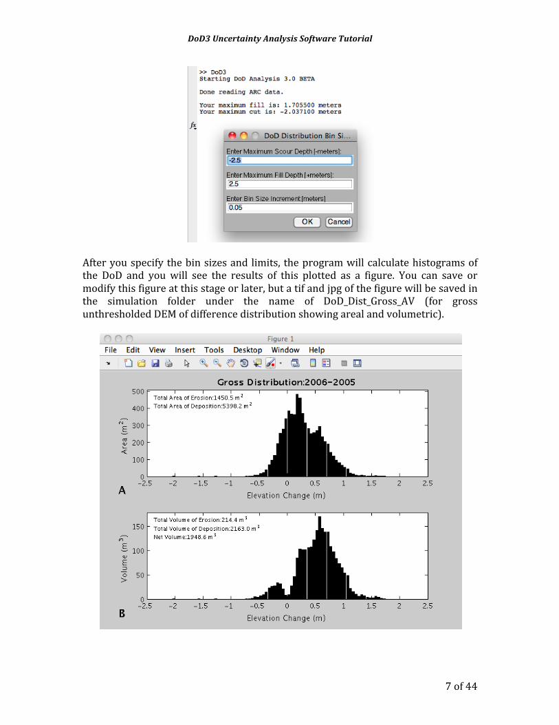
After you load your two DEMs or a DEM of Difference (DoD), the maximum fill depth and cut depth in meters are reported in the Matlab command window. This is done so that you have a basis for selecting appropriate limits for your histogram. The default is +/-‐ 2.5 meters, which works well for many fluvial settings. However, if you want your histogram to span your entire range of elevation change values, you should double check what gets reported in the command window. The other critical parameter here is the bin size increment, which is set at a default of 5 cm. Too fine of an increment can produce discontinuous looking distributions, whereas too coarse of an increment can produce a very blocky histogram.
DoD3 Uncertainty Analysis Software Tutorial
7 of 44
After you specify the bin sizes and limits, the program will calculate histograms of the DoD and you will see the results of this plotted as a figure. You can save or modify this figure at this stage or later, but a tif and jpg of the figure will be saved in the simulation folder under the name of DoD_Dist_Gross_AV (for gross unthresholded DEM of difference distribution showing areal and volumetric).

DoD3 Uncertainty Analysis Software Tutorial
8 of 44
It is worth taking a moment to explain what these elevation change distributions (ECDs) are showing as the ECDs are one of the primary outputs used to summarize the various forms of DoD analyses. The top plot (A) is an areal ECD and shows the distribution of elevation change in terms of surface area experiencing each magnitude of elevation change. The shape of this distribution is the same as what you’d see if you looked at a histogram of raster values for the DoD, but instead of the vertical axis being a cell count, it has been multiplied by the cell area (raster resolution) to show the proportion of the surface experiencing what types of change. It is very common for a majority or high percentage of the surface to be centered around zero representing a combination of no change, minimal change and/or noise. The total area of erosion (i.e. the integral of the area under curve to the left of 0), and the total area of deposition (i.e. the integral of the area under curve to the right of 0) are reported in the upper left corner. The bottom plot (B) is a volumetric ECD and shows the distribution of elevation change in terms of a volume of mass moved (either by net erosion or net deposition). The vertical axis values have been determined by multiplying the area in each bin by the central value of elevation change in that bin. The result is that the shape of the distribution can be quite different, because low magnitude changes are modulated and large magnitude changes are amplified. The volumetric distributions are more helpful in terms of geomorphic sediment budgeting, because they represent the net amount of work done (presumably by geomorphic change) as a change in storage (volume in this case). The total volume of erosion and deposition are reported in the upper right hand corners as well as the difference of the two, which gives an indication whether the whole area within the ECD is net-‐aggradational or net depositional, or in net balance. From this point your responses to the next dialogs determine your pathway, so navigate ahead to the next appropriate subsection. Next you will be asked whether you want to consider Uncertainty in the DoD. If you choose ‘Skip’, this is a Pathway 1 analysis. For Pathways 2 through 6, choose ‘Continue’.
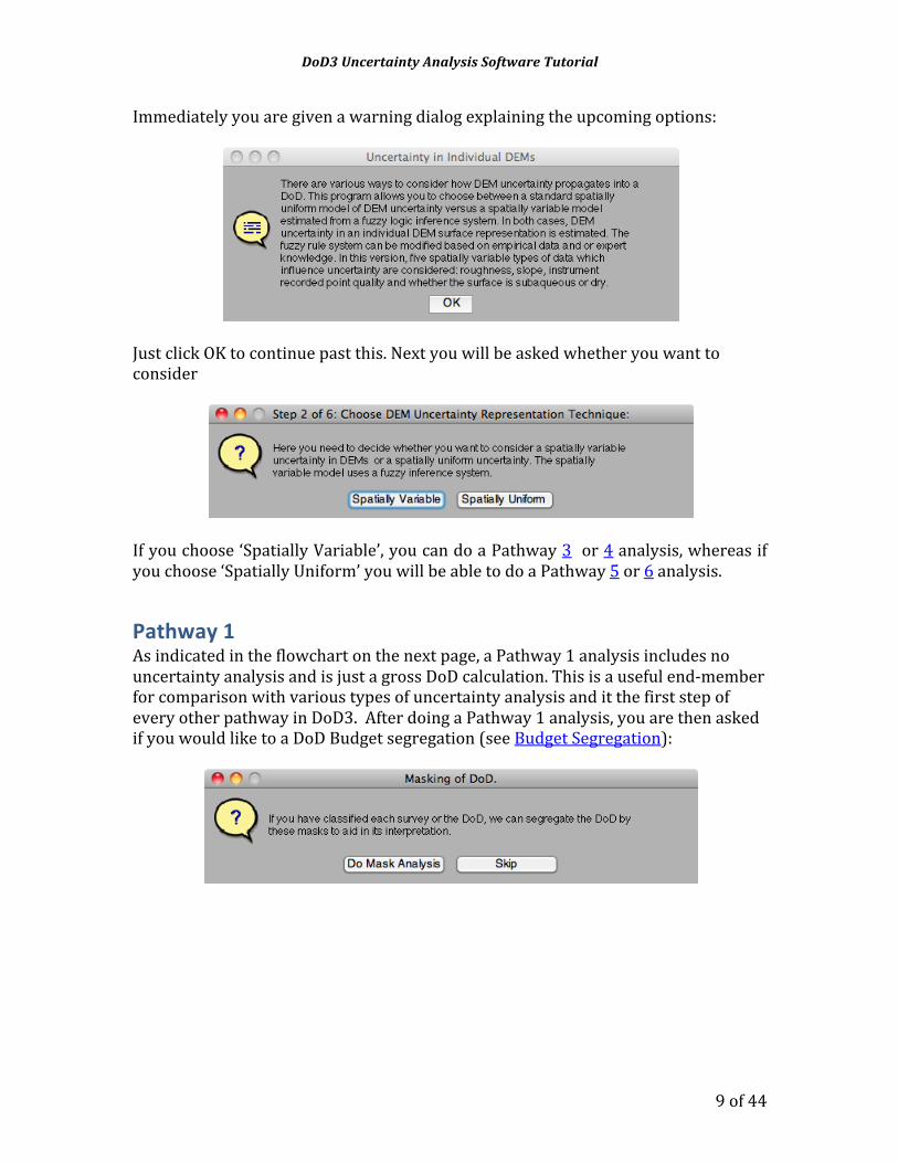
The first choice is whether to do a simple (elevation threshold based) uncertainty analysis or a more sophisticated probabilistic uncertainty analysis. If you choose a ‘Simple’, this is the equivalent of Pathway 2 Analysis. If you choose ‘More Sophisticated’, this will allow a Pathway 3, 4, 5 or 6 analysis.
DoD3 Uncertainty Analysis Software Tutorial
9 of 44
Immediately you are given a warning dialog explaining the upcoming options:
Just click OK to continue past this. Next you will be asked whether you want to consider
If you choose ‘Spatially Variable’, you can do a Pathway 3 or 4 analysis, whereas if you choose ‘Spatially Uniform’ you will be able to do a Pathway 5 or 6 analysis.
Pathway 1 As indicated in the flowchart on the next page, a Pathway 1 analysis includes no uncertainty analysis and is just a gross DoD calculation. This is a useful end-‐member for comparison with various types of uncertainty analysis and it the first step of every other pathway in DoD3. After doing a Pathway 1 analysis, you are then asked if you would like to a DoD Budget segregation (see Budget Segregation):

DoD3 Uncertainty Analysis Software Tutorial
10 of 44
Pathway 1 Analysis in DoD3
START:DEM of Difference Analysis Program
Run DoD Segregation
Analyses
0.0
0.5
1.0
1.5
2.0
2.5
3.0
3.5
4.0
Visualize DoD Distributionsaccording to geomorphic segregation?
Input Parameters can Include:1. Slope; 2. Point Density; 3. 3D Point Quality; 4. Roughness & 5. Wet Dry (note: all grids contain continuous variables)
FINISH
Produce Final Report& Output Data Files
ConsiderUncertainty
in DoD?YES IGNORE
Type ofUncertainty
AnalysisSIMPLE(DoD)
MORESOPHISTICATED
(Individual DEMs)
IsUncertainty
SpatiallyVariable?NO YES
YES
CREATE
NO
YES
Load or Create
DoD
Create DoD from2 Input DEMs
Load Existing DoD
CalculateGrossDoD
Save DoDfor Later Use?
0.0
0.5
1.0
1.5
2.0
2.5
3.0
3.5
4.0
?
? Visualize DoDDistribution?
Consider a SimpleminLoD ElevationThreshold for DoD
Assign SpatiallyUniform Elevation
Uncertainty for Each DEMLoad
or CreateFIS Uncertainty
Estimate
Create FIS from Input Parameters for Each DEM
Load Existing FISFor Each DEM
Apply Fuzzy InferenceSystem to Produce
Estimate of Elevation Uncertainty
(on a cell-by-cell basis)
Save FIS Gridsfor Later Use?
Propagate Elevation Uncertainty from each DEM
into DoD Calculation(on a cell-by-cell basis)
?
?
?
?
?
Convert PropagatedUncertainty to a Probability that Predicted DoD Change
is Real(on a cell-by-cell basis)
Loador Create
NeighbourhoodCoherence
Grid?
Load Existing NeighbourhoodGrid
Moving WindowAnalysis of Spatial
Coherence of Erosion & Deposition Patterns
(on a cell-by-cell basis)
Save NeighbourhoodGrid for Later Use?
ConsiderSpatial
Coherence inDoD?
?
Use Previous Probability as a Priori Estimate, and convert Neighbourhood
Analysis to Probability. Apply Bayes Theorem to provide updated Probability
that predicted DoD change is Real(on a cell-by-cell basis)
Save ProbabilityGrids for Later Use?
Save Updated ProbabilityGrids for Later Use?
Apply MinimumLevel of DetectionThreshold to DoD
Choose ConfidenceInterval to Apply
Threshold to DoD(Probability)
Save Thresholded DoDfor Later Use?
0.0
0.5
1.0
1.5
2.0
2.5
3.0
3.5
4.0?Visualize Thresholded DoD Distributions?
NO
PerformGeomorphic
Segregation ofDoD?
?
Load SegregationMask(s)

DoD3 Uncertainty Analysis Software Tutorial
11 of 44
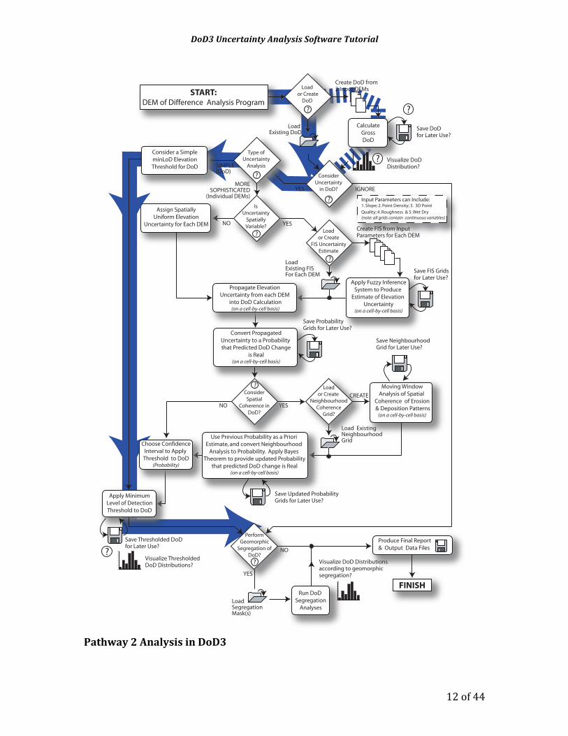
Pathway 2 A pathway 2 analysis is the simplest form of uncertainty analysis allowed in this program. This is a simple application of a spatially uniform minimum level of detection (in meters). You are simply asked to specify the value of your minimum level of detection in a dialog. For more information on how these values are reasonably arrived at, see Wheaton (2008, chapter 4). The next step is to Threshold your DoD based on this value (see DoD Thresholding). The flowchart on the next page illustrates the pathway.
DoD3 Uncertainty Analysis Software Tutorial
12 of 44
Pathway 2 Analysis in DoD3
START:DEM of Difference Analysis Program
Run DoD Segregation
Analyses
0.0
0.5
1.0
1.5
2.0
2.5
3.0
3.5
4.0
Visualize DoD Distributionsaccording to geomorphic segregation?
Input Parameters can Include:1. Slope; 2. Point Density; 3. 3D Point Quality; 4. Roughness & 5. Wet Dry (note: all grids contain continuous variables)
FINISH
Produce Final Report& Output Data Files
ConsiderUncertainty
in DoD?YES IGNORE
Type ofUncertainty
AnalysisSIMPLE(DoD)
MORESOPHISTICATED
(Individual DEMs)
IsUncertainty
SpatiallyVariable?NO YES
YES
CREATE
NO
YES
Load or Create
DoD
Create DoD from2 Input DEMs
Load Existing DoD
CalculateGrossDoD
Save DoDfor Later Use?
0.0
0.5
1.0
1.5
2.0
2.5
3.0
3.5
4.0
?
? Visualize DoDDistribution?
Consider a SimpleminLoD ElevationThreshold for DoD
Assign SpatiallyUniform Elevation
Uncertainty for Each DEMLoad
or CreateFIS Uncertainty
Estimate
Create FIS from Input Parameters for Each DEM
Load Existing FISFor Each DEM
Apply Fuzzy InferenceSystem to Produce
Estimate of Elevation Uncertainty
(on a cell-by-cell basis)
Save FIS Gridsfor Later Use?
Propagate Elevation Uncertainty from each DEM
into DoD Calculation(on a cell-by-cell basis)
?
?
?
?
?
Convert PropagatedUncertainty to a Probability that Predicted DoD Change
is Real(on a cell-by-cell basis)
Loador Create
NeighbourhoodCoherence
Grid?
Load Existing NeighbourhoodGrid
Moving WindowAnalysis of Spatial
Coherence of Erosion & Deposition Patterns
(on a cell-by-cell basis)
Save NeighbourhoodGrid for Later Use?
ConsiderSpatial
Coherence inDoD?
?
Use Previous Probability as a Priori Estimate, and convert Neighbourhood
Analysis to Probability. Apply Bayes Theorem to provide updated Probability
that predicted DoD change is Real(on a cell-by-cell basis)
Save ProbabilityGrids for Later Use?
Save Updated ProbabilityGrids for Later Use?
Apply MinimumLevel of DetectionThreshold to DoD
Choose ConfidenceInterval to Apply
Threshold to DoD(Probability)
Save Thresholded DoDfor Later Use?
0.0
0.5
1.0
1.5
2.0
2.5
3.0
3.5
4.0?Visualize Thresholded DoD Distributions?
NO
PerformGeomorphic
Segregation ofDoD?
?
Load SegregationMask(s)

DoD3 Uncertainty Analysis Software Tutorial
13 of 44
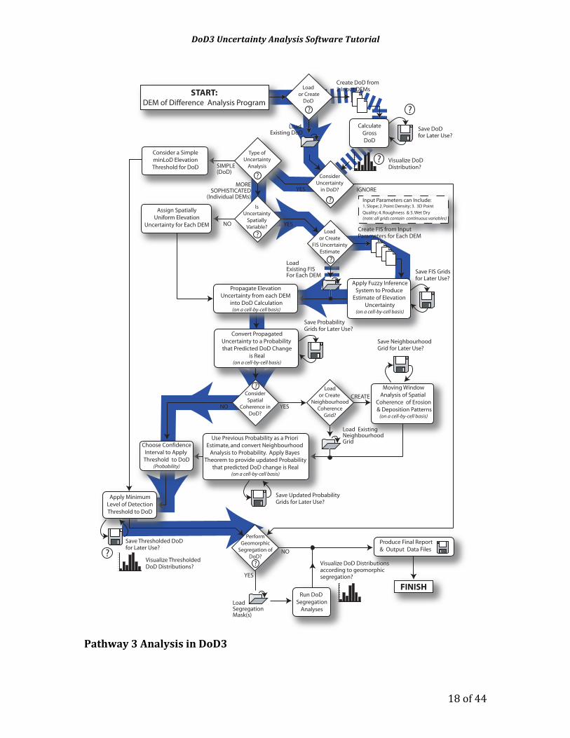
Pathway 3 In a pathway 3 analysis, you are using a fuzzy inference system (FIS) to estimate the surface representation uncertainty of your DEMs on a cell by cell basis in each DEM (see flow chart at end of this section). Thus, this is a spatially variable analysis. A separate FIS estimate of elevation uncertainty is needed for both the newer DEM and the older DEM. As indicated below, you are given the option to either load a grid previously calculated (saves time) or to Create a New FIS. In this example, we will ‘Create a New FIS’ using our Sulphur Creek datasets.
A notification dialog appears explaining the process and warning you to be patient as the calculation can be slow:
The way a new FIS estimate of uncertainty is calculated depends on what input data you have available. This version1 of the program has built into it rules systems calibrated for GPS and total station surveys with various combinations of five potential inputs. The two mandatory inputs are slope and point density (see readme file), whereas roughness (in meters), 3D GPS point quality (in meters) and water depth (in meters) are all optional. For many topographic surveys, these defaults will likely work well, but you may wish to calibrate, modify or extend the FIS using the fuzzy logic toolbox (see here for more information). The way the program knows which FIS is to use, is based on what inputs you tell it you have and load a grid for. We start with slope analysis:
1 Later versions of DoD3 (currently under development) will include the option to use FIS systems for airborne LiDaR (green and Near-‐IR), aerial photogrammetry, and ground-‐based LiDaR in addition to total station and GPS surveys. See readme for more information.

DoD3 Uncertainty Analysis Software Tutorial
14 of 44
Answer yes to this question and you will be asked to load the ‘2006 Slope Analysis’ grid in our example (the more recent survey). You can find this in the ‘2006Feb’ folder within the Input folder and named ‘2006Feb_SA.asc’:
After this has loaded, you are asked if you want to load a point density grid from 2006 (for this example).
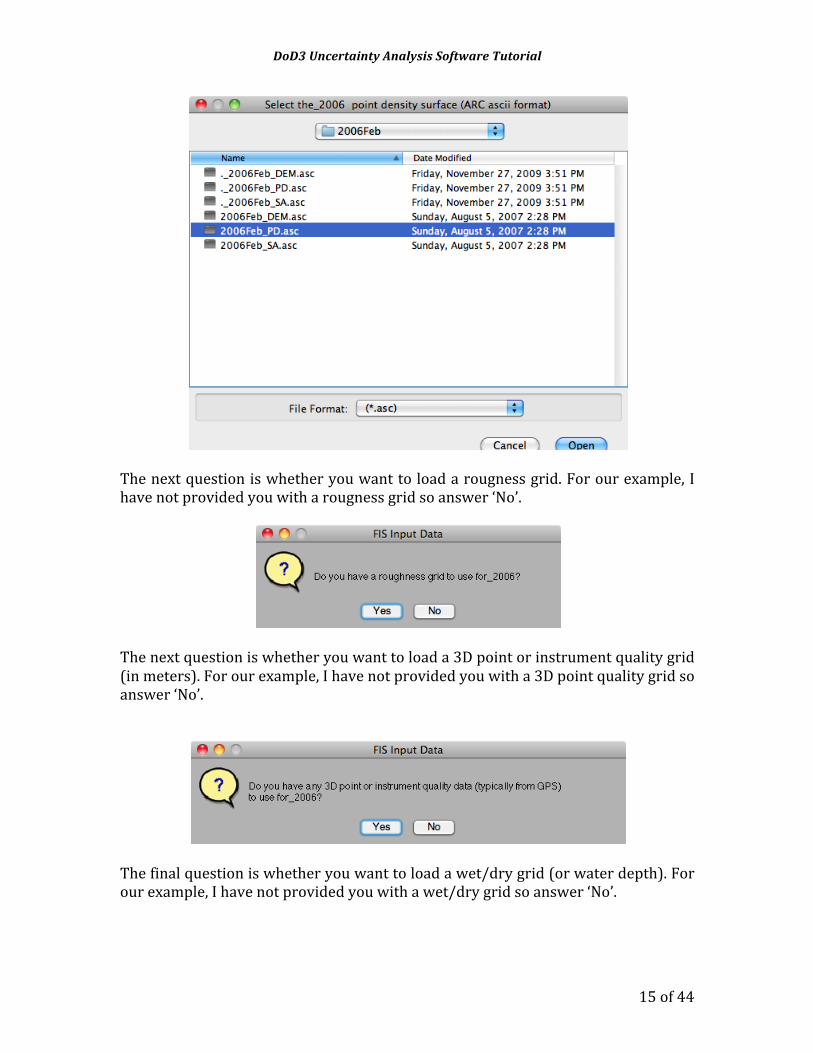
Again, answer yes and you will be asked to load the ‘2006 Point Density Surface’ grid (calculated in points per square meter). You can find this in the ‘2006Feb’ folder within the Input folder and named ‘2006Feb_PD.asc’:
DoD3 Uncertainty Analysis Software Tutorial
15 of 44
The next question is whether you want to load a rougness grid. For our example, I have not provided you with a rougness grid so answer ‘No’.
The next question is whether you want to load a 3D point or instrument quality grid (in meters). For our example, I have not provided you with a 3D point quality grid so answer ‘No’.
The final question is whether you want to load a wet/dry grid (or water depth). For our example, I have not provided you with a wet/dry grid so answer ‘No’.

DoD3 Uncertainty Analysis Software Tutorial
16 of 44
If all you wanted to do is calculate these FIS grids, you can save the FIS grids and quit out of the program at this stage. If you wish to proceed with your Pathway 3 or Pathway 4 analysis, click ‘Save and Continue’ (do not click ‘Help’… there is none).
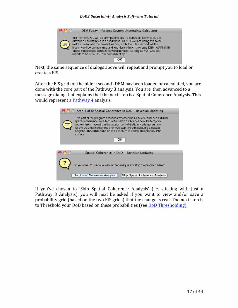
After answering this last question, you will notice that Matlab is busy and it may take some time for it to complete the calculation of the FIS grid. Do not be alarmed if a warning message appears at the command prompt notifying you some of the input values are outside the specified input range of the FIS (such cells will be ignored). When the process is complete a message dialog informs you that you are done with the analysis for the newer DEM and need to repeat the steps for the older DEM:
Click ‘OK’ to proceed.
DoD3 Uncertainty Analysis Software Tutorial
17 of 44
Next, the same sequence of dialogs above will repeat and prompt you to load or create a FIS. After the FIS grid for the older (second) DEM has been loaded or calculated, you are done with the core part of the Pathway 3 analysis. You are then advanced to a message dialog that explains that the next step is a Spatial Coherence Analysis. This would represent a Pathway 4 analysis.
If you’ve chosen to ‘Skip Spatial Coherence Analysis’ (i.e. sticking with just a Pathway 3 Analysis), you will next be asked if you want to view and/or save a probability grid (based on the two FIS grids) that the change is real. The next step is to Threshold your DoD based on these probabilities (see DoD Thresholding).
DoD3 Uncertainty Analysis Software Tutorial
18 of 44
Pathway 3 Analysis in DoD3
START:DEM of Difference Analysis Program
Run DoD Segregation
Analyses
0.0
0.5
1.0
1.5
2.0
2.5
3.0
3.5
4.0
Visualize DoD Distributionsaccording to geomorphic segregation?
Input Parameters can Include:1. Slope; 2. Point Density; 3. 3D Point Quality; 4. Roughness & 5. Wet Dry (note: all grids contain continuous variables)
FINISH
Produce Final Report& Output Data Files
ConsiderUncertainty
in DoD?YES IGNORE
Type ofUncertainty
AnalysisSIMPLE(DoD)
MORESOPHISTICATED
(Individual DEMs)
IsUncertainty
SpatiallyVariable?NO YES
YES
CREATE
NO
YES
Load or Create
DoD
Create DoD from2 Input DEMs
Load Existing DoD
CalculateGrossDoD
Save DoDfor Later Use?
0.0
0.5
1.0
1.5
2.0
2.5
3.0
3.5
4.0
?
? Visualize DoDDistribution?
Consider a SimpleminLoD ElevationThreshold for DoD
Assign SpatiallyUniform Elevation
Uncertainty for Each DEMLoad
or CreateFIS Uncertainty
Estimate
Create FIS from Input Parameters for Each DEM
Load Existing FISFor Each DEM
Apply Fuzzy InferenceSystem to Produce
Estimate of Elevation Uncertainty
(on a cell-by-cell basis)
Save FIS Gridsfor Later Use?
Propagate Elevation Uncertainty from each DEM
into DoD Calculation(on a cell-by-cell basis)
?
?
?
?
?
Convert PropagatedUncertainty to a Probability that Predicted DoD Change
is Real(on a cell-by-cell basis)
Loador Create
NeighbourhoodCoherence
Grid?
Load Existing NeighbourhoodGrid
Moving WindowAnalysis of Spatial
Coherence of Erosion & Deposition Patterns
(on a cell-by-cell basis)
Save NeighbourhoodGrid for Later Use?
ConsiderSpatial
Coherence inDoD?
?
Use Previous Probability as a Priori Estimate, and convert Neighbourhood
Analysis to Probability. Apply Bayes Theorem to provide updated Probability
that predicted DoD change is Real(on a cell-by-cell basis)
Save ProbabilityGrids for Later Use?
Save Updated ProbabilityGrids for Later Use?
Apply MinimumLevel of DetectionThreshold to DoD
Choose ConfidenceInterval to Apply
Threshold to DoD(Probability)
Save Thresholded DoDfor Later Use?
0.0
0.5
1.0
1.5
2.0
2.5
3.0
3.5
4.0?Visualize Thresholded DoD Distributions?
NO
PerformGeomorphic
Segregation ofDoD?
?
Load SegregationMask(s)
DoD3 Uncertainty Analysis Software Tutorial
19 of 44
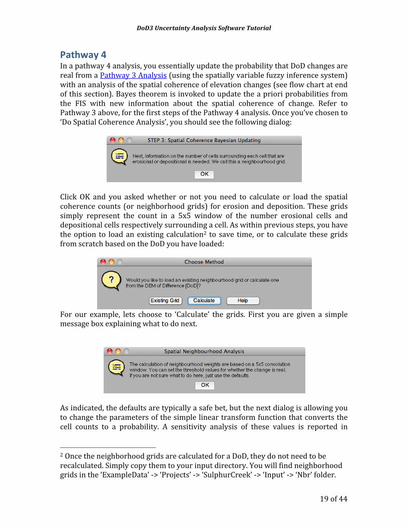
Pathway 4 In a pathway 4 analysis, you essentially update the probability that DoD changes are real from a Pathway 3 Analysis (using the spatially variable fuzzy inference system) with an analysis of the spatial coherence of elevation changes (see flow chart at end of this section). Bayes theorem is invoked to update the a priori probabilities from the FIS with new information about the spatial coherence of change. Refer to Pathway 3 above, for the first steps of the Pathway 4 analysis. Once you’ve chosen to ‘Do Spatial Coherence Analysis’, you should see the following dialog:
Click OK and you asked whether or not you need to calculate or load the spatial coherence counts (or neighborhood grids) for erosion and deposition. These grids simply represent the count in a 5x5 window of the number erosional cells and depositional cells respectively surrounding a cell. As within previous steps, you have the option to load an existing calculation2 to save time, or to calculate these grids from scratch based on the DoD you have loaded:
For our example, lets choose to ‘Calculate’ the grids. First you are given a simple message box explaining what to do next.
As indicated, the defaults are typically a safe bet, but the next dialog is allowing you to change the parameters of the simple linear transform function that converts the cell counts to a probability. A sensitivity analysis of these values is reported in
2 Once the neighborhood grids are calculated for a DoD, they do not need to be recalculated. Simply copy them to your input directory. You will find neighborhood grids in the ‘ExampleData’ -‐> ‘Projects’ -‐> ‘SulphurCreek’ -‐> ‘Input’ -‐> ‘Nbr’ folder.

DoD3 Uncertainty Analysis Software Tutorial
20 of 44
Chapter 4 of Wheaton (2008), but your upper limit should not exceed 25. For this example, just use the default values.
When the calculations are finished, you are given the following message dialog (same dialog appears whether you have loaded or calculated neighborhood grids).
Next you are given the option to view (with a Matlab figure) the probability surfaces created with these analyses. The a Priori is the result of the FIS system, and the Posterior is the result of the Pathway 4 analysis. I typically click ‘No’ here.
If you do instead click ‘Yes’, you will see two figures produced. I would not suggest modifying these figures or zooming in on them until after the program has completed running. At that point you can then modify and save them. The values produced are probabilities. Positive values are probabilities of deposition being real, whereas negative probabilities are probabilities of erosion being real.

DoD3 Uncertainty Analysis Software Tutorial
21 of 44
You then have the option to save both the a priori and posterior probability grids to an Ascii raster file. If you choose yes (recommended), these grids will be saved to your ‘OutputRasters’ folder for the simulation (see Project File Management) and you can visualize them later.
The next step is to Threshold your DoD based on these probabilities (see DoD Thresholding).

DoD3 Uncertainty Analysis Software Tutorial
22 of 44
START:DEM of Difference Analysis Program
Run DoD Segregation
Analyses
0.0
0.5
1.0
1.5
2.0
2.5
3.0
3.5
4.0
Visualize DoD Distributionsaccording to geomorphic segregation?
Input Parameters can Include:1. Slope; 2. Point Density; 3. 3D Point Quality; 4. Roughness & 5. Wet Dry (note: all grids contain continuous variables)
FINISH
Produce Final Report& Output Data Files
ConsiderUncertainty
in DoD?YES IGNORE
Type ofUncertainty
AnalysisSIMPLE(DoD)
MORESOPHISTICATED
(Individual DEMs)
IsUncertainty
SpatiallyVariable?NO YES
YES
CREATE
NO
YES
Load or Create
DoD
Create DoD from2 Input DEMs
Load Existing DoD
CalculateGrossDoD
Save DoDfor Later Use?
0.0
0.5
1.0
1.5
2.0
2.5
3.0
3.5
4.0
?
? Visualize DoDDistribution?
Consider a SimpleminLoD ElevationThreshold for DoD
Assign SpatiallyUniform Elevation
Uncertainty for Each DEMLoad
or CreateFIS Uncertainty
Estimate
Create FIS from Input Parameters for Each DEM
Load Existing FISFor Each DEM
Apply Fuzzy InferenceSystem to Produce
Estimate of Elevation Uncertainty
(on a cell-by-cell basis)
Save FIS Gridsfor Later Use?
Propagate Elevation Uncertainty from each DEM
into DoD Calculation(on a cell-by-cell basis)
?
?
?
?
?
Convert PropagatedUncertainty to a Probability that Predicted DoD Change
is Real(on a cell-by-cell basis)
Loador Create
NeighbourhoodCoherence
Grid?
Load Existing NeighbourhoodGrid
Moving WindowAnalysis of Spatial
Coherence of Erosion & Deposition Patterns
(on a cell-by-cell basis)
Save NeighbourhoodGrid for Later Use?
ConsiderSpatial
Coherence inDoD?
?
Use Previous Probability as a Priori Estimate, and convert Neighbourhood
Analysis to Probability. Apply Bayes Theorem to provide updated Probability
that predicted DoD change is Real(on a cell-by-cell basis)
Save ProbabilityGrids for Later Use?
Save Updated ProbabilityGrids for Later Use?
Apply MinimumLevel of DetectionThreshold to DoD
Choose ConfidenceInterval to Apply
Threshold to DoD(Probability)
Save Thresholded DoDfor Later Use?
0.0
0.5
1.0
1.5
2.0
2.5
3.0
3.5
4.0?Visualize Thresholded DoD Distributions?
NO
PerformGeomorphic
Segregation ofDoD?
?
Load SegregationMask(s)
DoD3 Uncertainty Analysis Software Tutorial
23 of 44
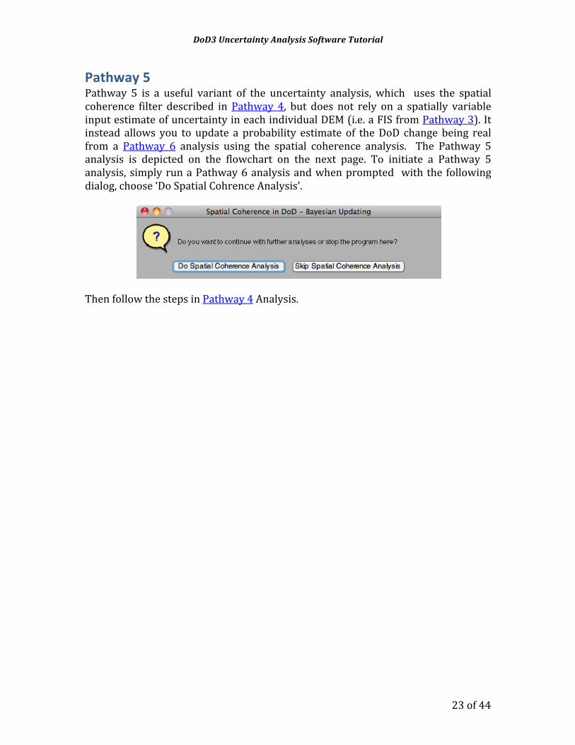
Pathway 5 Pathway 5 is a useful variant of the uncertainty analysis, which uses the spatial coherence filter described in Pathway 4, but does not rely on a spatially variable input estimate of uncertainty in each individual DEM (i.e. a FIS from Pathway 3). It instead allows you to update a probability estimate of the DoD change being real from a Pathway 6 analysis using the spatial coherence analysis. The Pathway 5 analysis is depicted on the flowchart on the next page. To initiate a Pathway 5 analysis, simply run a Pathway 6 analysis and when prompted with the following dialog, choose ‘Do Spatial Cohrence Analysis’.
Then follow the steps in Pathway 4 Analysis.

DoD3 Uncertainty Analysis Software Tutorial
24 of 44
START:DEM of Difference Analysis Program
Run DoD Segregation
Analyses
0.0
0.5
1.0
1.5
2.0
2.5
3.0
3.5
4.0
Visualize DoD Distributionsaccording to geomorphic segregation?
Input Parameters can Include:1. Slope; 2. Point Density; 3. 3D Point Quality; 4. Roughness & 5. Wet Dry (note: all grids contain continuous variables)
FINISH
Produce Final Report& Output Data Files
ConsiderUncertainty
in DoD?YES IGNORE
Type ofUncertainty
AnalysisSIMPLE(DoD)
MORESOPHISTICATED
(Individual DEMs)
IsUncertainty
SpatiallyVariable?NO YES
YES
CREATE
NO
YES
Load or Create
DoD
Create DoD from2 Input DEMs
Load Existing DoD
CalculateGrossDoD
Save DoDfor Later Use?
0.0
0.5
1.0
1.5
2.0
2.5
3.0
3.5
4.0
?
? Visualize DoDDistribution?
Consider a SimpleminLoD ElevationThreshold for DoD
Assign SpatiallyUniform Elevation
Uncertainty for Each DEMLoad
or CreateFIS Uncertainty
Estimate
Create FIS from Input Parameters for Each DEM
Load Existing FISFor Each DEM
Apply Fuzzy InferenceSystem to Produce
Estimate of Elevation Uncertainty
(on a cell-by-cell basis)
Save FIS Gridsfor Later Use?
Propagate Elevation Uncertainty from each DEM
into DoD Calculation(on a cell-by-cell basis)
?
?
?
?
?
Convert PropagatedUncertainty to a Probability that Predicted DoD Change
is Real(on a cell-by-cell basis)
Loador Create
NeighbourhoodCoherence
Grid?
Load Existing NeighbourhoodGrid
Moving WindowAnalysis of Spatial
Coherence of Erosion & Deposition Patterns
(on a cell-by-cell basis)
Save NeighbourhoodGrid for Later Use?
ConsiderSpatial
Coherence inDoD?
?
Use Previous Probability as a Priori Estimate, and convert Neighbourhood
Analysis to Probability. Apply Bayes Theorem to provide updated Probability
that predicted DoD change is Real(on a cell-by-cell basis)
Save ProbabilityGrids for Later Use?
Save Updated ProbabilityGrids for Later Use?
Apply MinimumLevel of DetectionThreshold to DoD
Choose ConfidenceInterval to Apply
Threshold to DoD(Probability)
Save Thresholded DoDfor Later Use?
0.0
0.5
1.0
1.5
2.0
2.5
3.0
3.5
4.0?Visualize Thresholded DoD Distributions?
NO
PerformGeomorphic
Segregation ofDoD?
?
Load SegregationMask(s)
DoD3 Uncertainty Analysis Software Tutorial
25 of 44
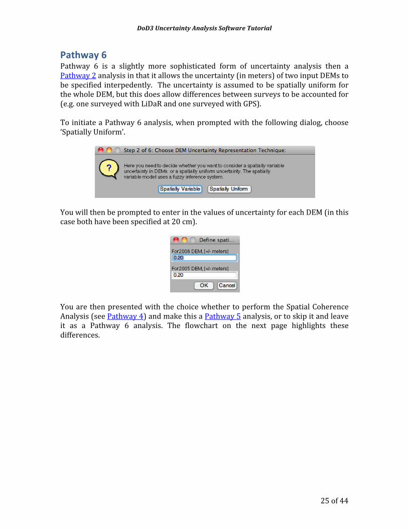
Pathway 6 Pathway 6 is a slightly more sophisticated form of uncertainty analysis then a Pathway 2 analysis in that it allows the uncertainty (in meters) of two input DEMs to be specified interpedently. The uncertainty is assumed to be spatially uniform for the whole DEM, but this does allow differences between surveys to be accounted for (e.g. one surveyed with LiDaR and one surveyed with GPS). To initiate a Pathway 6 analysis, when prompted with the following dialog, choose ‘Spatially Uniform’.
You will then be prompted to enter in the values of uncertainty for each DEM (in this case both have been specified at 20 cm).
You are then presented with the choice whether to perform the Spatial Coherence Analysis (see Pathway 4) and make this a Pathway 5 analysis, or to skip it and leave it as a Pathway 6 analysis. The flowchart on the next page highlights these differences.

DoD3 Uncertainty Analysis Software Tutorial
26 of 44
START:DEM of Difference Analysis Program
Run DoD Segregation
Analyses
0.0
0.5
1.0
1.5
2.0
2.5
3.0
3.5
4.0
Visualize DoD Distributionsaccording to geomorphic segregation?
Input Parameters can Include:1. Slope; 2. Point Density; 3. 3D Point Quality; 4. Roughness & 5. Wet Dry (note: all grids contain continuous variables)
FINISH
Produce Final Report& Output Data Files
ConsiderUncertainty
in DoD?YES IGNORE
Type ofUncertainty
AnalysisSIMPLE(DoD)
MORESOPHISTICATED
(Individual DEMs)
IsUncertainty
SpatiallyVariable?NO YES
YES
CREATE
NO
YES
Load or Create
DoD
Create DoD from2 Input DEMs
Load Existing DoD
CalculateGrossDoD
Save DoDfor Later Use?
0.0
0.5
1.0
1.5
2.0
2.5
3.0
3.5
4.0
?
? Visualize DoDDistribution?
Consider a SimpleminLoD ElevationThreshold for DoD
Assign SpatiallyUniform Elevation
Uncertainty for Each DEMLoad
or CreateFIS Uncertainty
Estimate
Create FIS from Input Parameters for Each DEM
Load Existing FISFor Each DEM
Apply Fuzzy InferenceSystem to Produce
Estimate of Elevation Uncertainty
(on a cell-by-cell basis)
Save FIS Gridsfor Later Use?
Propagate Elevation Uncertainty from each DEM
into DoD Calculation(on a cell-by-cell basis)
?
?
?
?
?
Convert PropagatedUncertainty to a Probability that Predicted DoD Change
is Real(on a cell-by-cell basis)
Loador Create
NeighbourhoodCoherence
Grid?
Load Existing NeighbourhoodGrid
Moving WindowAnalysis of Spatial
Coherence of Erosion & Deposition Patterns
(on a cell-by-cell basis)
Save NeighbourhoodGrid for Later Use?
ConsiderSpatial
Coherence inDoD?
?
Use Previous Probability as a Priori Estimate, and convert Neighbourhood
Analysis to Probability. Apply Bayes Theorem to provide updated Probability
that predicted DoD change is Real(on a cell-by-cell basis)
Save ProbabilityGrids for Later Use?
Save Updated ProbabilityGrids for Later Use?
Apply MinimumLevel of DetectionThreshold to DoD
Choose ConfidenceInterval to Apply
Threshold to DoD(Probability)
Save Thresholded DoDfor Later Use?
0.0
0.5
1.0
1.5
2.0
2.5
3.0
3.5
4.0?Visualize Thresholded DoD Distributions?
NO
PerformGeomorphic
Segregation ofDoD?
?
Load SegregationMask(s)

DoD3 Uncertainty Analysis Software Tutorial
27 of 44
DoD Thresholding Once you have your best estimate of the uncertainty in a DoD, you can use that information to threshold the DoD. This process is described in both Wheaton et al. (2009) and Wheaton (2008, Chapter 4) in detail. Briefly, either an elevation change minimum level of detection is defined (i.e. Pathway 2 or Pathway 6) or a probabilistic minimum level of detection is defined (i.e a confidence interval from Pathway 3, 4 or 5). Then the cells in the original DoD with values beneath these thresholds are changed from their original values to no-‐data cells (i.e. they are threshold out or removed on the basis that they can not be distinguished from noise). When you reach this step of the program you will see an informational dialog as follows:
If you used Pathway 2 or 6, the thresholding may be automatic, but if you used pathways 3, 4 or 5, you will see a dialog asking you for a value between 0 and 1 (i.e. the decimal probability) you wish to threshold at. Obviously, a higher value is a more conservative estimate, and a lower value is more liberal.
After the thresholding is complete, you are asked if you would like to save an Ascii raster of your thresholded DoD (recommended). If you choose to, this grid will be stored in your ‘OutputRasters’ folder.
A useful way of comparing the influence of DoD analysis is to compare the elevation change distribution (ECD) of the original DoD with that of the thresholded DoD. The next step asks you whether you wish to do this analysis (recommended).

DoD3 Uncertainty Analysis Software Tutorial
28 of 44
If you choose to ‘Do Analysis’, a figure will be produced similar to below. A *.jpg and *.tif of the same figure are saved in your simulation folder. If you did a Pathway 4 or 5 analysis, using the spatial coherence filter, you will also be prompted to do this twice (once for the a priori ECD and once for the posterior ECD). At the end of the analysis, you can modify and/or save these figure(s).
Budget Segregation Budget segregation is described extensively in Chapter 5 of Wheaton (2009). In a nutshell, once you have your best estimate of DoD changes (i.e. a thresholded DoD from Pathway 2, 3, 4, 5 or 6 analysis), you then use spatial masks (i.e. polygons) to quantify how much change has taken place in discrete spatial locations. To run, the

DoD3 Uncertainty Analysis Software Tutorial
29 of 44
polygons need to be converted to rasters with a unique integer corresponding to each category (see Project File Management and the ExampleData for examples). The budget segregation is one of the last steps to the DoD3 program (optional), or it can be run as a stand alone application (using A_Geomorph.m) as shown below.
There are two types of mask analyses possible. The simple mask uses a single input mask to segregate the polygon. The Classification of Difference (CoD) mask asks for two classification masks (typically one of the older DEM and one of the newer DEM) and then calculates unique categories of change (to use as masks) from the difference between the two classifications. Below we will walk through a simple example using data from Sulphur Creek. Note that CoD examples can also be found in the ‘Example Data’ -‐> ‘Projects’ -‐> ‘SulphurCreek’ -‐> ‘Input’ -‐> ‘Geomorph’ -‐> ‘GoD’ folder. Assuming we are entering the Mask Analysis from the DoD3 program, you are then asked if you would like to a DoD Budget segregation:
?
START 1: Direct From DoD Analysis Program
START 1: Direct From DoD Analysis Program
START 2: Stand-AlonePost-Processing
Run Stats& SaveOutput Reports
0.0
0.5
1.0
1.5
2.0
2.5
3.0
3.5
4.0
Visualize DoD Distributionsaccording to Mask
FINISH
Produce Final Report& Output Data Files
YES
CLASSIFICATIONOF DIFFERENCE (CoD)
SIMPLE MASK
START 2
STA
RT 1
DoD Uncertainty Software
ChooseMaskType
IF
CalculateUnicque CoD
Classes From Inputs
NO
PerformGeomorphic
Segregation ofDoD?
?
Load 2 IndividualClassification Masks
Load SegregationMask(s)
Use Mask(s) to SegregateDoD Spatially into individual
Mask Classes
Save CoDGrids for Later Use?

DoD3 Uncertainty Analysis Software Tutorial
30 of 44
If you choose to ‘Skip’ the masking or budget segregation step, the Final Report (see here) is then produced and you are asked if you would like to view the final thresholded DoD. Choose ‘Do Mask Analysis’ for our example. As it is possible and typical to segregate the same DoD budget in a variety of ways, you can repeat this geomorphic analysis (using the ‘A_Geomorph.m’ program’). Accordingly, here you are prompted to enter a name for your masking analysis. This will create a folder (of the same name) in a ‘Geomorph’ subdirectory of your simulation.
You are then prompted to specify what type of segregation you are going to do. In our example we will do a simple mask, so use ‘Mask’:
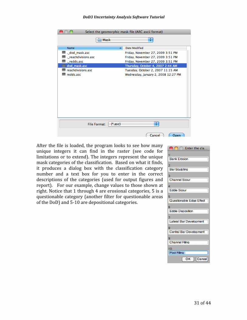
You are then prompted to load the input mask you wish to use. We will load a file called ‘dod_mask.asc’, which can be found in ‘Example Data’ -‐> ‘Projects’ -‐> ‘SulphurCreek’ -‐> ‘Input’ -‐> ‘Geomorph’ -‐> ‘Mask’. This mask is reported in Chapter 6 of Wheaton (2008) and a figure can be found below showing the mask. It represents a gemorphic interpretation of the change from a combination of DoD interpretation, field evidence and repeat aerial photography.
DoD3 Uncertainty Analysis Software Tutorial
31 of 44
After the file is loaded, the program looks to see how many unique integers it can find in the raster (see code for limitations or to extend). The integers represent the unique mask categories of the classification. Based on what it finds, it produces a dialog box with the classification category number and a text box for you to enter in the correct descriptions of the categories (used for output figures and report). For our example, change values to those shown at right. Notice that 1 through 4 are erosional categories, 5 is a questionable category (another filter for questionable areas of the DoD) and 5-‐10 are depositional categories.

DoD3 Uncertainty Analysis Software Tutorial
32 of 44
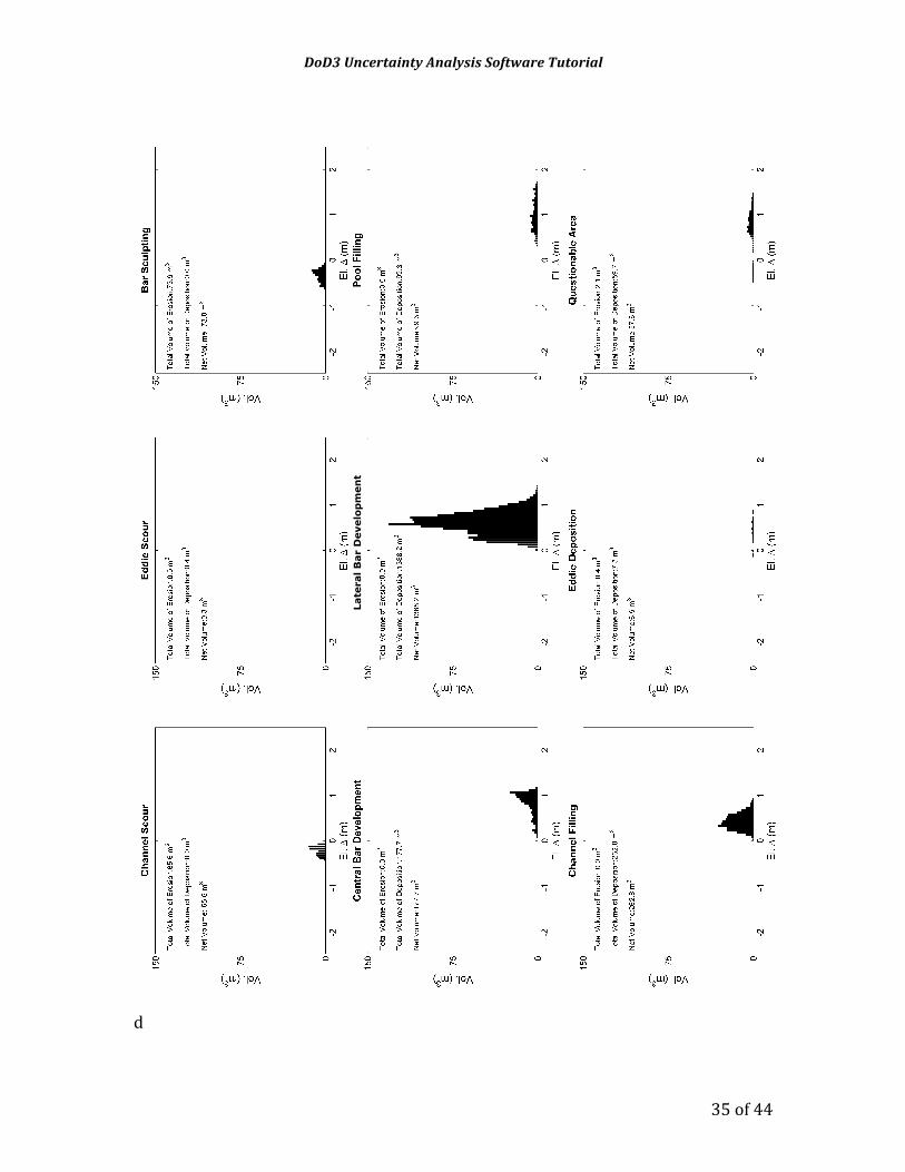
The portion labeled as ‘A’ of the figure at right shows the classification mask we are loading in this example. The portion labeled as B is a pie chart showing one summary of the masking analysis. Here the total volume of change has been divided by the volume of change in each category to determine what category was responsible for producing the most change (i.e. geomorphic work). In this example, lateral bar development dominates. These and other analyses can be summarized from a *.csv file in the output folder that has the ‘_Summary.csv’ suffix.
0 10 20 30 40 50Meters
Legend
Analysis Extent
O
Mask
Classification ofDifference (CoD)
A
B
Bank Erosion
Bar Sculpting
Channel Scour
Eddie Scour
Questionable Edge Effect
Eddie Deposition
Lateral Bar Development
Central Bar Development
Channel Filling
Pool Filling
Percentages by Mask Classes of Total Volume of Sediment Moved
66%
5%
12%
0%3%0%
3%0%
8%
3%

DoD3 Uncertainty Analysis Software Tutorial
33 of 44
What happens is that elevation change distributions are calculated for each category. Two figures for each are produced, 1) a combined plot showing the areal and volumetric ECD; and 2) a plot showing just the volumetric ECD with a common maximum volume for the ECD to allow easier inter-‐comparison (you’ll see the benefits of this in the figures below). Thus, the next dialog prompts you to enter in this maximum fill volume for the second ECD. A good rule of thumb is to use 50% of the maximum volume on the vertical axis of the unthresholded DoD ECD. It may take some trial and error to arrive an appropriate value. In our example, just use the default 150 cubic meter value:
You will then see the program cycle through its production of all the ECD plots (be patient). It saves *.jpgs and *.tiffs of each as well as a *.csv file of each. The combined areal and volumetric figures look something like below:
Notice that the vertical axis is scaled to whatever the peak values of the ECD are and the text label at the top of the figure comes from that which was entered in the earlier dialog for the categories. The second figure that gets produced has its vertical

DoD3 Uncertainty Analysis Software Tutorial
34 of 44
axis set to the value, which was specified (150 in this example). And just shows the volumetric ECD. Notice that the distribution looks much smaller when plotted like this.
The utility of this becomes apparent in the figure shown on the next page. The figure shows an intercomparison of 9 of the 10 categories of change defined by the masks. It allows for an easy identification of the dominant categories of change as well as highlighting distinctive signatures of change.
DoD3 Uncertainty Analysis Software Tutorial
35 of 44
d
Late
ral
Bar
Develo
pm
en
t

DoD3 Uncertainty Analysis Software Tutorial
36 of 44
Final Report At the end of any successful DoD3 analysis, the program attempts to produce several outputs to assist you in later interpretation or reanalysis of the results. When you see the dialog below, you know you’ve successfully reached this point.
Depending on what Pathway you chose, different outputs are reported. All will have a DoD_MetaDataReport.txt and a file with the ‘_ElevDist.csv’ suffix as well as a ‘BatchParamters.csv file. The ‘_ElevDist.csv’ file contains a comma separate file showing all the outputs of the various ECDs of the DoD produced. This enables you to load the data into any other program for subsequent analysis of the ECD or to make your own custom figures. The ‘BatchParametrs.csv’ file contains all the parameters necessary to rerun the exact same analysis (see Batch Processing section for more information). On the next page an example of a portion of the ‘DoD_MetaDataReport.txt’ is shown. The report is intended to provide a summary of the analyses conducted to aid you in later interpretation of simulation results.

DoD3 Uncertainty Analysis Software Tutorial
37 of 44
Batch Processing It is not uncommon to want to perform a sensitivity analysis of the uncertainty analysis to varying parameters. Every simulation produced with the DoD3 program produces an output file called ‘BatchParamters.csv’. This file has a header row with the parameter names and a second row with the parameter values for that simulation. You can rerun any simulation by simply starting DoD3, running it in batch mode and reading this file.

DoD3 Uncertainty Analysis Software Tutorial
38 of 44
Alternatively, you can run numerous simulations in a batch processing mode by editing this file to have multiple rows. You can call your batch simulation file anything you wish while saving it as a *.csv file. I recommend saving this in your Input directory. An example is provided (see Project File Management). Each row will have a different suite of parameter values (for example, minimally it will have different simulation names). The batch program then goes through and runs each simulation in order. The best way to see how to properly format the batch file is to run a regular wizard mode simulation of the type of pathway you whish to run. Then copy the row from that BatchParameters.csv file to the *.csv file you are producing for batch processing and edit them from there.
Project File Management As mentioned above, you can specify your project folder to sit any where on your machine or network that Matlab can see. A sample project folder has been provided for you in the ExampleData folder in the zip file. Note that in this case the project folder is ‘SulphurCreek’ and not ‘Projects’. You could choose to put multiple projects in the the ‘Projects’ folder.
Within every project folder that DoD3 runs on, there will always be an ‘Input’ folder and a ‘Simulations’ folder. In the data provided to you, only the ‘Input’ folder exists initially, but after one DoD3 analysis, the ‘Simulations’ folder will appear.
The Input Folder For many projects, you will run a wide range of analyses off a relatively small set of input data. Instead of duplicating this input data and copying into each simulation folder, that input data can be housed in one place. The ‘Input’ folder is required for this. Where ever you are asked in DoD3 to load data, it defaults to point the open file dialog to this ‘Input’ folder. You can organize your input data in anyway you wish (i.e. with any naming convention and with or without subdirectories). As an

DoD3 Uncertainty Analysis Software Tutorial
39 of 44
example, we will describe how the input data are organized for the SulphurCreek example below:
At the root level in this input folder we have only three files:
• 2006 Feb-2005 Dec_DoD.asc : An ascii raster DoD between February 2006 and December 2005
• PW4_BatchSA.csv : This is an example of a batch processing input file (for running DoD3 in batch mode) for a pathway 4 sensitivity analysis (NOTE: this would need to be updated to work on your machine, because the file paths will be incorrect)
• PW4_Multiplot.dat : This is an example of a multi-‐plot input file for use with the A_MultDistPlot tool (note: this would need to have the path and simulation folder names updated to work)
Within the subfolders, we have a variety of folders:
• 2005Dec – This folder contains the DEM raster and the point density and slope analysis input rasters for the FIS from 2005
• 2006Feb – Same types of rasters as above but for 2006 • FIS – This folder contains the raster output of a FIS analysis using the 2-‐rule
point density and slope analysis data (these can be called up from DoD3 once they are run once, instead of re-‐running them each time… much quicker)
• Geomorph

DoD3 Uncertainty Analysis Software Tutorial
40 of 44
o GoD – Contains a geomorphic classification of difference input rasters (for 3 and 10 category classifications)
o Mask – Contains three types of DoD Masks (a geomorphic interpretation, a sub-‐reach mask, and a Chinook redd mask)
• Nbr – The spatial coherence grids for erosion and deposition for the 2006-‐2005 DoD (these too can be called up from DoD3 once they are run once, instead of re-‐running them each time… much quicker)
The Simulation Folder Depending on the type of analysis you run and the answers to the wizard questions, you will have different contents in your simulation folders. Each simulation (or analysis) you run will have it own subfolder in the Simulation folder. Below we show the contents of a simulation called ‘Analysis PW2’:
Within the that folder we see some common files and subfolders:
• BatchParameters.csv: This CSV file gets created every time you run a simulation and is a complete record of all the parameters used to run that simulation. It can be used in batch mode to repeat an analysis, or by copying the rows (e.g. in excel) and modifying the correct parameters it can be used to batch process numerous simulations.
• DoD_Dist_Gross_AV (jpg & tif) – These are just image files of the gross elevation change distributions (ECDs) with no uncertainty accounting
• DoD_Dist_PW2_AV – These are image files of gross ECDs with a pathway 2 analysis
• DoD_MetaDataReport.txt – This is the text file output report, which summarizes all of the analyses
• Geomorph folder – This where all masking analyses get outputted. Note that in this case there is a CoD_A folder (Classification of Difference A). You can

DoD3 Uncertainty Analysis Software Tutorial
41 of 44
and often do run multiple masks over the same DoD analysis and these would each get stored in here as different subdirectories.
• Output Rasters folder – This is where any output rasters created during your analysis get stored. These include your thresholded DoD rasters, FIS output rasters, spatial coherence output rasters, DoD probability maps, etc. Although you can view these rasters in Matlab, typically, these rasters are best visualized in another stand-‐alone GIS application.
• P2DoDElevDist.csv file – This CSV file gets outputted from every analysis and contains the raw data to produce the histograms of all the elevation change distributions associated with that simulation. This can be used to make your own figures in any program (e.g. Excel, or using some of the analysis tools here in Matlab)

DoD3 Uncertainty Analysis Software Tutorial
42 of 44
Matlab Scripts & Functions – Program Folder Within the ‘Programs’ folder, you will find a mix *.m Matlab script and function files and *.fis fuzzy inference files. The naming convention for the *.m files is as follows:
• DoD3.m is the main program file to access the wizard program or batch processing version.
• All *.m files with the ‘A_’ prefix are analysis programs, some of which are called from DoD3 and some of which can be run as stand-‐alone files on outputs from DoD3
• The handful of *.m files with the ‘f_’ prefix are functions
• All *.m files with the ‘io_’ prefix are scripts for reading in data from files and writing output data to files (primarily ASCII raster grids).
• Any *.m file with a ‘m_’ prefix is one of the primary method scripts called in DoD3
The *.fis files are created using the fuzzy logic toolbox. If you wish to change the existing membership functions or rules (but keep the same inputs), you can do this manually in the *.fis files or with the help the fuzzy logic toolbox’s GUI. If you wish to extend the fuzzy inference system, you will need to create a new *.fis using the fuzzy logic toolbox and then update the calls to this *.fis within the m_2DEM_FIS.m file (line 47 updates the call to the *.fis file). You will also need to update the io_Reader_FIS_Inputs.m file to add additional inputs.

DoD3 Uncertainty Analysis Software Tutorial
43 of 44
Some notes about the Code You will notice that pretty much everything loaded or calculated gets stored in memory. This was done partly to make code development easier and have flexibility in pathway. It is however very inefficient. When you’re working with smaller rasters (i.e. less then 100 MB) with a machine with more than 2GB RAM, this tends not to be a problem. However, with larger rasters you may exceed your memory limits. You can insert lines in your code to clear some of the unnecessary grids from Matlab’s memory.3 Another inefficient feature of the code is the use of ascii text rasters. These are much slower to read in and write out then binary raster formats. However, ascii raster formats are readable buy a wide variety of other programs and are nice for troubleshooting because you can read them with any text editor (e.g. notepad). As Matlab is a non-‐complied language, it is very slow at running loops. Where possible, the code has been vectorized to speed it up. However, there are certain grid operations we could not get to work as easily or flexibly and have left these in loops. This is again an inefficient feature of the code. The above shortcomings are all part of the reasons the program is being parsed over into a compiled C++ library, which will drive a platform independent web application and an ArcGIS plugin (toolbar). However, for many users who might only make slight modifications to the sourecode, this Matlab version should be relatively straightforward to follow and or modify.
3 The C++ library version under development will be much more memory efficient and quicker

DoD3 Uncertainty Analysis Software Tutorial
44 of 44
Matlab Version Notes: This program was originally developed in Matlab 6 running in Windows XP Pro, and this release was tested and in Matlab 7.8.0.347 (R2009a) on Mac OSX 10.6.2. There have been minor syntax differences between older and newer releases. If running an older version, you may need to edit the code. If you are attempting to run this without the Fuzzy Logic Toolbox installed, the code will crash in Pathways 3 & 4.
References: Wheaton JM. 2008. Uncertainty in Morphological Sediment Budgeting of Rivers.
Unpublished PhD, University of Southampton, Southampton, 412 pp. Available at: http://www.joewheaton.org.uk/Research/Projects/PhDThesis.asp.
Wheaton JM, Brasington J, Darby SE and Sear D. 2009. Accounting for uncertainty in DEMs from repeat topographic surveys: Improved sediment budgets Earth Surface Processes and Landforms. 34. DOI: 10.1002/esp.1886.

DoD 3.0 Beta Read Me DEM of Difference Uncertainty Analysis Software
Produced by Joe Wheaton Copyright (C) 2009 Wheaton Developer can be contacted at [email protected] or Joe Wheaton, Department of Watershed Sciences, Utah State University, 5210 Old Main Hill, Logan, UT 84322-‐5210, USA. This program is free software; you can redistribute it and/or modify it under the terms of the GNU General Public License as published by the Free Software Foundation; either version 2 of the License, or (at your option) any later version. This program is distributed in the hope that it will be useful, but WITHOUT ANY WARRANTY; without even the implied warranty of MERCHANTABILITY or FITNESS FOR A PARTICULAR PURPOSE. See the GNU General Public License for more details. You should have received a copy of the GNU General Public License along with this program; if not, write to the Free Software Foundation, Inc., 51 Franklin Street, Fifth Floor, Boston, MA 02110-‐1301 USA or see http://www.gnu.org/licenses/gpl-‐2.0.txt (GLP v2 license). If you do choose to modify the source code and redistribute it, please cite the Wheaton et al. (2009b) paper accordingly. Updated November 1, 2009 WHAT DOES IT DO? The DoD3 software was developed primarily for morphological sediment budgeting in rivers. The volumetric change in storage is calculated from the difference in surface elevations from digital elevation models (DEMs) derived from repeat topographic surveys. As each DEM has an uncertain surface representation (which might vary in space and time), DoD3 provides a suite of tools for quantifying those uncertainties and propagating them through to the DEM of difference. The program also provides ways for segregating the best estimates change spatially using different types of masks. The overall suite of tools is more generically applicable to many different spatial change detection problems. BACKGROUND Thank you for downloading our DoD 3.0 Beta Software. This release was made available to accompany a paper published in Earth Surface Processes and Landforms. It is a fully functioning Matlab version of the code, which was used in the ESPL paper (Wheaton et al., 2009b), the Wheaton (2008) thesis, and the Wheaton et al. (2009a) RRA paper. This code is provided as supplemental information with the ESPL paper so that readers can test or extend the code as they see fit for their purposes. Together with the paper and Wheaton (2008) thesis (particularly Chapters, 4 and 5), this readme and a tutorial act as the documentation for this version of the source code. The tutorial file is intended to help walk you through application of the code. Additionally, some sample input data used in Chapter 6 of the Wheaton (2008) thesis is provided to show you how the input data should be pre-‐processed and so you can compare the outputs with the analyses published there. The code has

reasonably verbose comments to help you follow along what its doing, however the main interface is a wizard driven dialog, that prompts you to enter your inputs and specify your preferences for the analyses. Based on the answers to your questions, you can work your way through the multiple pathways outlined in Chapter four of the Wheaton (2008) thesis (for reference, pathways 3 & 4 are what are reported in the ESPL paper). Alternatively, you can skip the verbose instructions and just cut right to running DoD3 from a command line in Matlab, and then just refer back to the tutorial if you get stuck. USER REQUIREMENTS: Some understanding of DEM differencing Familiarity with Matlab
SYSTEM REQUIREMENTS: Matlab 7 or later (tested on 7.8.0.347 (R2009a) on Mac OSX 10.6.2) Fuzzy Logic Toolbox for Matlab Machine with enough RAM to handle your input rasters
INPUT DATA REQUIREMENTS: Everything you need to run this software can be derived from a raw x-‐y-‐z
point cloud of your topographic survey data. From this you can build a TIN and derive a raster DEM. You can also derive a point density grid and slope analysis (the only two required inputs for the fuzzy inference system)
Input data are on collinear rasters of equal extent and resolution and in an Arc ASCII format (see example input files); the headers should be identical
Data are assumed to be in meters and on the same vertical datum Inputs to Fuzzy Inference system:
o If you use slope input rasters, slope should be calculated as a percent slope
o If you use point density rasters, point density should be calculated in points per square meter
o If you use roughness input rasters, roughness heights should be reported in meters
o If you use 3D GPS Point quality input rasters, quality should be reported in meters
o If you use water depth input rasters, depth should be reported in meters
Inputs to Geomorphic Interpretation / Masking o Whether you use the classification of difference method or straight
masking method, the input masks should be raster integer grids with 1, 2, 3, … n corresponding to unique mask categories (you will be prompted to enter what linguistic categories these values correspond to)

INSTALLATION PROCEDURE: To start, unzip the contents of DoD3_Beta using folder names to a desired location visible by Matlab. There are three folders: Documentation -‐> contains readme, tutorial and license files Programs -‐> contains all the Matlab scripts and functions that collectively
comprise the program ExampleData -‐> Contains some sample data from Sulphur Creek California
for you to use to become familiar with the program and compare your results with Chapter 6 of Wheaton (2008).
The vast majority of analyses available to you are accessed from running the DoD3.m file in the Progam directory (see ‘Matlab Scipts & Function – Program Folder’ section of DoD3_Tutorial File for more info). Below are the three folders found in the root of the zip file:
FUTURE RELEASES, SUPPORT & UPDATES: The DoD software is under ongoing development. That development is extending the software to other survey technologies, capability of handling larger raster sizes, and other change detection problems. At the time of this release, the code is being refactored into an open-‐source C++ library, which will be the backbone to a web-‐application and an ArcGIS plug-‐in. However, this Matlab version of the software is perfectly functional and should be easily extendible to users familiar with Matlab. Given the ease of development within Matlab, we felt it was important to make this version of the code available to others. Future releases will just be of the C++ library, and will automatically apply to the web-‐application that anyone will be able to use without proprietary Matlab or ArcGIS software licenses. No formal support is available with this free software, but you can always contact the developer if you have questions or suggestions. Good luck. REFERENCES: Wheaton JM. 2008. Uncertainty in Morphological Sediment Budgeting of Rivers.
Unpublished PhD, University of Southampton, Southampton, 412 pp.

Available at: http://www.joewheaton.org.uk/Research/Projects/PhDThesis.asp.
Wheaton JM, Brasington J, Darby SE, Merz JE, Pasternack GB, Sear DA and Vericat D. 2009a. Linking Geomorphic Changes to Salmonid Habitat at a Scale Relevant to Fish. River Research and Applications. DOI: 10.1002/rra.1305.
Wheaton JM, Brasington J, Darby SE and Sear D. 2009b. Accounting for uncertainty in DEMs from repeat topographic surveys: Improved sediment budgets Earth Surface Processes and Landforms. 34. DOI: 10.1002/esp.1886.
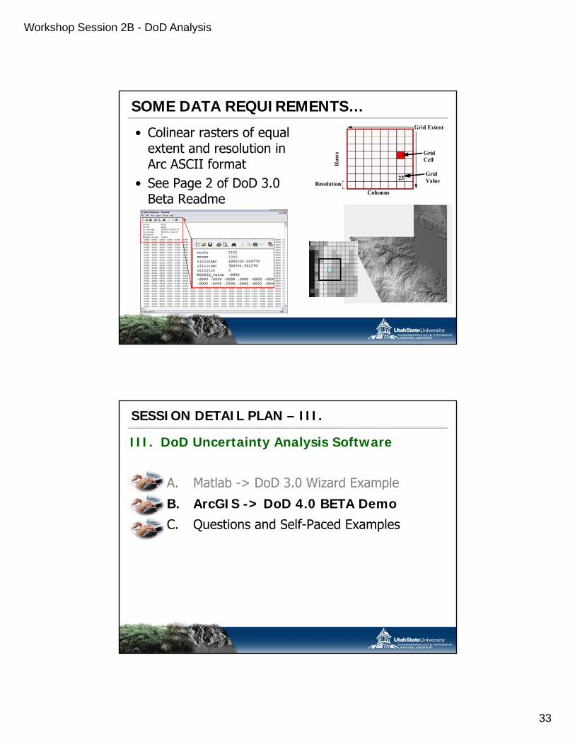
Workshop Session 2B - DoD Analysis
33
SOME DATA REQUIREMENTS…
• Colinear rasters of equal extent and resolution in Arc ASCII format
• See Page 2 of DoD 3.0 Beta Readme
SESSION DETAIL PLAN – III.
III. DoD Uncertainty Analysis Software
A Matlab -> DoD 3 0 Wizard ExampleA. Matlab > DoD 3.0 Wizard Example
B. ArcGIS -> DoD 4.0 BETA DemoC. Questions and Self-Paced Examples

Workshop Session 2B - DoD Analysis
34
DoD 4.0… NO PATHWAYS, JUST ArcGIS
Just a quick demo of things to come…
DoD 4.0 – Other Versions
• C++ Source Code (dll)F ti lit b d i• Functionality can be accessed using:– Stand-alone Windows GUI Version– Command Prompt utilities (from Linux, Mac or
Windows)– Web Application (browser-based, reduced
functionality)u ct o a ty)

Workshop Session 2B - DoD Analysis
35
SESSION DETAIL PLAN – III.
III. DoD Uncertainty Analysis Software
A Matlab -> DoD 3 0 Wizard ExampleA. Matlab > DoD 3.0 Wizard Example
B. ArcGIS -> DoD 4.0 BETA Demo
C. Questions and Self-Paced Examples
SESSION PLAN…
I. Introduction / review of DEM Differencing
II Alternative approaches to
1:05 to 1:20ish
II. Alternative approaches to accounting for DEM uncertainty
III. DoD Uncertainty Analysis Software
1:20 to 2:00ish
2:00 to 2:45ish
IV. Interpreting DoDs 2:45 to 3:15ish

Workshop Session 2B - DoD Analysis
36
WHAT MORE CAN WE SAY OR ASK?
Best estimate of gross reach-scale sediment budget
Deposition Volume 1156.1 4810.8 1288.5 6605.3Erosion Volume 2268.1 5794.0 1857.8 8581.0Net -1112.0 -983.2 -569.3 -1975.7
e.g. What is the dominant mechanism of change?
Where in the reach is contributing the most?
LET’S SAY MORE…
1. Reliability Uncertainty:Of the predicted changes, what can we actually distinguish
z Z Z DEMActual
from noise?
t
zz
t
zz
We want:
But,
2. Structural Uncertainty:Geomorphically, what do the calculated changes mean?

Workshop Session 2B - DoD Analysis
37
USE MASKS TO SEGREGATE DoD
What are the individual mechanisms of net change?
ARTICULATE THE ARM-WAVING AS MASK
• Qualitative geomorphic interpretations pare easy (and useful)
• Translate these to quantitative analyses by using asusing as classification mask for DoD segregation

Workshop Session 2B - DoD Analysis
38
SESSION DETAIL PLAN – IV.
IV. Interpreting DoDs
A. How to interpret DoDs using masksB Si l hi i t t ti lB. Simple geomorphic interpretation example
THREE TYPES OF MASKS
Just a way of spatially segregating budget to ask questions and query
Segregates both DoD & its Elevation Change Distribution…
q q ybudget results.
1.Standard Classification2.Classification of
Difference3 Geomorphic3.Geomorphic
InterpretationJust polygons…

Workshop Session 2B - DoD Analysis
39
1. STANDARD CLASSIFCATION
• Any classification that is of:– The pre-survey– The post-survey– Or Time Independent
• Examples:– Morphological Units– Habitat Classification– Administrative Bndys– Reaches
2. CLASSIFICATION OF DIFFERENCE
• The difference is defined by all possible combinations of class change or stabilitychange or stability
• Same classification used for earlier and later surveys
• Good for looking at correlation between geomorphic change andgeomorphic change and categorical change
• The N2 problem

Workshop Session 2B - DoD Analysis
40
CoD APPLIED…
• The largest class was in a stable class (bar to bar)to bar)
• Inferences about processes can be made (i.e. bar to channel erosional)
3. GEOMORPHIC INTERPRETATION
• Instead of mask being based on one point in time, this is based on the change surface it lf (i th D D)itself (i.e. the DoD)
• Multiple lines of evidence can be used beyond DoD
• You define geomorphic processes of interest

Workshop Session 2B - DoD Analysis
41
DOMINANT OR UNIQUE SIGNATURES?
THREE DIFFERENT WAYS OF INTERPRETING SAME DoD• Are the conclusions contradictory?• Does the spatial
masking/segregation tell usClassification of DifferenceClassification of Difference
Standard Classification
Standard Classification
masking/segregation tell us something that the gross analysis can not?
• Does this allow for more explicit and quantitative hypothesis testing?
• Are unique or distinctive signatures f h (i ECD ) ? Understanding of
Geomorphic InterpretationGeomorphic
Interpretation
of change (in ECDs) present?• Sensitivity to single interpretation..
Understanding of DoD Budget

Workshop Session 2B - DoD Analysis
42
TRANSFORMING UNCERTAINTY?• Considered in terms of sources• Provides a rationale for treating
different sources differently• Some can be transformed• Some can be transformed
Figure Adapted from Van Asselt and Rotmans (2002): http://dx.doi.org/10.1023/A:1015783803445
SESSION DETAIL PLAN – IV.
IV. Interpreting DoDs
A. How to interpret DoDs using masks
B Si l hi i t t tiB. Simple geomorphic interpretation example

Workshop Session 2B - DoD Analysis
43
REFER TO DoD 3.0 TUTORIAL
SESSION REVIEW…
I. Introduction / review of DEM Differencing
II Alternative approaches to
1:05 to 1:20ish
II. Alternative approaches to accounting for DEM uncertainty
III. DoD Uncertainty Analysis Software
1:20 to 2:00ish
2:00 to 2:45ish
IV. Interpreting DoDs 2:45 to 3:15ish

Workshop Session 2B - DoD Analysis
44
ONGOING SOFTWARE DEVELOPMENT• Finish DoD 4.0 for ArcGIS & Stand-Alone, finish help
documentation (next few months)• Extend FIS ‘rule of thumb’ library to other survey
technologiestechnologies– Green LiDaR, NIR LiDaR, TLS, Multi-beam SONAR, &
Optically-based depth retrievals (over next year)• DoD 4.0 – Web Application on OpenTopography.org
(over next year)• DoD 5.0 – A USGS GCMRC project
P i Cl d d P i h dli– Point Cloud and Pre-processing handling– Batch processing capability– Mixed input capability (e.g. LiDaR & multi-beam) – Inter-simulation comparisons
WHERE HAVE WE APPLIED THIS?• River Feshie, Scotland• River Rees, New Zealand• Bridge Creek, Oregon• Asotin Creek, Washington• Logan River, UT• Sulphur Creek, California• Mokelumne River, California• Yuba River, California• Highland Water England
In the next year:• Grand Canyon, Arizona• Yampa River, Colorado
Trinity River California• Highland Water, England• Provo River, Utah
• Trinity River, California• Lemhi River, Idaho• Salmon Falls Landslide, Idaho

Workshop Session 2B - DoD Analysis
45
WHAT’S THIS BEING USED FOR?• Long-term geomorphic monitoring & sediment budgeting
(e.g. Wheaton et al., 2010a)• Monitoring habitat & floodplain reconnection restoration
projects (e g Wheaton et al 2010b)projects (e.g. Wheaton et al., 2010b)• Monitoring feedbacks associated with beaver dams• Monitoring changes in fish habitat
QUESTIONS?
So do you understand:1. DoD techniques and how
they are applied to
DoD 3.0 & DoD 4.0
sediment budgets2. How to account for
unreliability uncertainties in DEMs
3. How to interpret DoDs
DoD = DEM of Difference =