1

EC109: Microeconomics I2019 – 2020

University of Warwick

Department of Economics

Terms 1 and 2

Professor Elizabeth Jones

Welcome!! This is the first part of a 2-year long microeconomics module:

EC109 and EC202 EC109 Module Leader: Professor Elizabeth Jones

Social Sciences S0.79 Elizabeth.H.Jones@warwick.ac.uk Advice and Feedback Hours: See my personal website

EC109 Lecturer: Dr. Andrew Harkins Social Sciences S1.113b Email Address: Andrew.Harkins@warwick.ac.uk Advice and Feedback Hours: See personal website

1

2

2

Organisation Lecture times (2 x 1 hour lectures) term 1:

Tuesday 2 – 3pm in R0.21

Thursday 12 – 1pm in OC1.05

Lecture times (2 x 1 hour lectures) term 2:

Tuesday 2 – 3pm in R0.21

Thursday 12 – 1pm in OC1.05

8 x 1 hour Workshops (fortnightly meetings weeks 3 – 10; 17 - 24)

8 x 1 hour classes (fortnightly meetings weeks 3 – 10; 17 - 24)

Sign up to a class time/group: stick to it

Only the UG office can give you permission to switch to another group (not your tutor)

Class/Workshop materials will be on the module webpage

Assessment 2 x Tests (20% in total)

One covering term 1 topics, worth 10%

One covering term 2 topics, worth 10%

Further details of time/location will be made available

New format this year – all MCQs

Exam (80%) Past papers available online

3

4

3

Resources The Syllabus

Lectures and the lecturers

Advice and Feedback hours: lecturers and tutors

Support and Feedback Classes and Class Tutors

Revision Sessions

Textbooks

Online resources

Forum

Tabula

Microeconomics Textbooks

‘Intermediate Microeconomics’ by Varian (WW Norton)

‘Microeconomics' by Perloff (Pearson) - easier

A suite of online resources is available if you purchase a new textbook with an access code

‘Game Theory: An Introduction’ by Tadelis (Princeton)

There are many other intermediate microeconomics textbooks that will cover the material – find one that suits you

5

6

4

Module Aims Across the two years, you will study a range of topics

and learn to Develop analysis which combines mathematical,

graphical and intuitive skills Apply theoretical concepts and analytical tools Understand how theoretical concepts can be applied

to various economic situations Develop critical analysis skills and an ability to question

rational economic thought Understand the policy implications of microeconomic

theory

Module Structure View EC109 as part 1 of your micro modules Topics are split between years 1 and 2 Aim: by the end of year 2, you can approach:

Mas-Colell’s ‘Microeconomic Theory’ or Varian’s ‘Microeconomic Analysis’

We start by showing you the final goal: where your studies of microeconomics can take you

1 lecture by a researcher in an area of applied microeconomics (8/10/19): Robbie Akerlof

Content is non-examinable, but link to and application of theory can be examined

7

8

5

The 2 year road map The plan for your 2 years in microeconomics

The core topics; The core skills; The tools of the trade

EC202

Choice under Uncertainty

Game Theory

General equilibrium

Market failure

EC109

Consumer Theory

Producer Theory

Market structure and firm behaviour

Intro to Game Theory

Partial equilibrium

EC109

CONSUMER THEORY

Elizabeth Jones

9

10

6

The Topics

Budget Constraints and the feasible set

Preferences

Indifference curves and utility functions

Revealed Preferences

Optimisation

Comparative statics

Changes in welfare

Applications

An example

If you and I go shopping in our respective local towns, why is it unlikely we will each come out of the shop with the same amount of each good in our baskets?

If I buy more milk than you, what are the possible explanations?

Differences in behaviour can emerge from

– Different tastes

– Different circumstances

We optimise subject to our constraints

11

12

7

BUDGET CONSTRAINTS

Budget constraint IIncome and prices affect the quantity consumers demand

– Income can be determined exogenously as an amount, M

– Or determined endogenously from resources

Assume my weekly income is £200 and I spend money on food at £5/g and clothes at £10/unit.

M= � × �� if I decide to only consume food.

200 = � × 5 → � = 40 =�

��

M= � × �� if I decide to only buy clothes.

200 = � × 10 → � = 20 =�

��

13

14

8

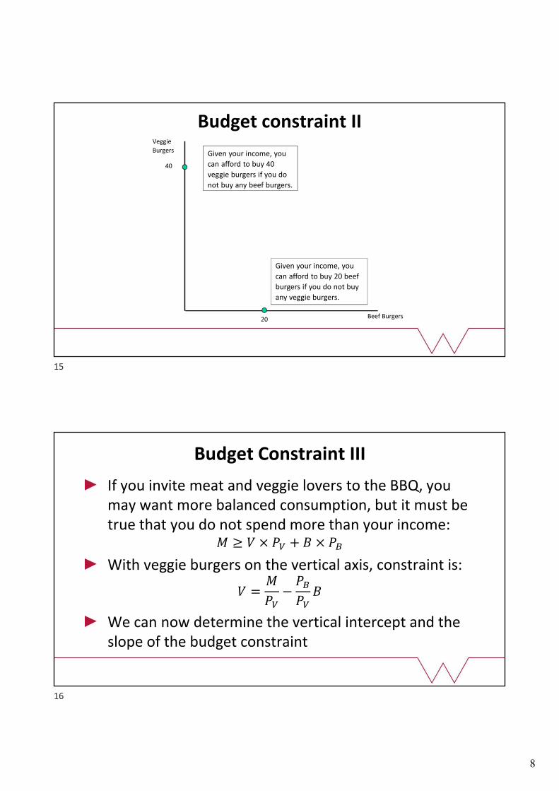
Budget constraint II

Given your income, you

can afford to buy 40

veggie burgers if you do

not buy any beef burgers.

Given your income, you

can afford to buy 20 beef

burgers if you do not buy

any veggie burgers.

Veggie

Burgers

Beef Burgers

40

20

If you invite meat and veggie lovers to the BBQ, you may want more balanced consumption, but it must be true that you do not spend more than your income:

� ≥ � × �� + � × ��

With veggie burgers on the vertical axis, constraint is:

� =�

��−

��

���

We can now determine the vertical intercept and the slope of the budget constraint

Budget Constraint III

15

16

9

The feasible set

Given your income, any

bundle below the budget

constraint is affordable.

Any bundle on the budget

constraint is just

affordable

Veggie

burgers

Beef Burgers

40

20

Plugging in the values for �, �� and �� allows us to construct the budget constraint and determine the feasible set:

200 = 5� + 10�

� =200

5−

10

5�

Budget constraint IV

The slope measures the rate the market ‘substitutes’ good 1 for good 2: it’s the opportunity cost of consuming good 1

If we consume more good 1, ∆��, by how much must good 2 change to continue to satisfy the budget constraint?

���� + ���� = �

��(�� + ∆��) + ��(�� + ∆��) = �

Subtract (1) from (2) to find: ��∆�� + ��∆�� = 0

Thus:∆��

∆��= −

��

��

(1)

(2)

17

18

10

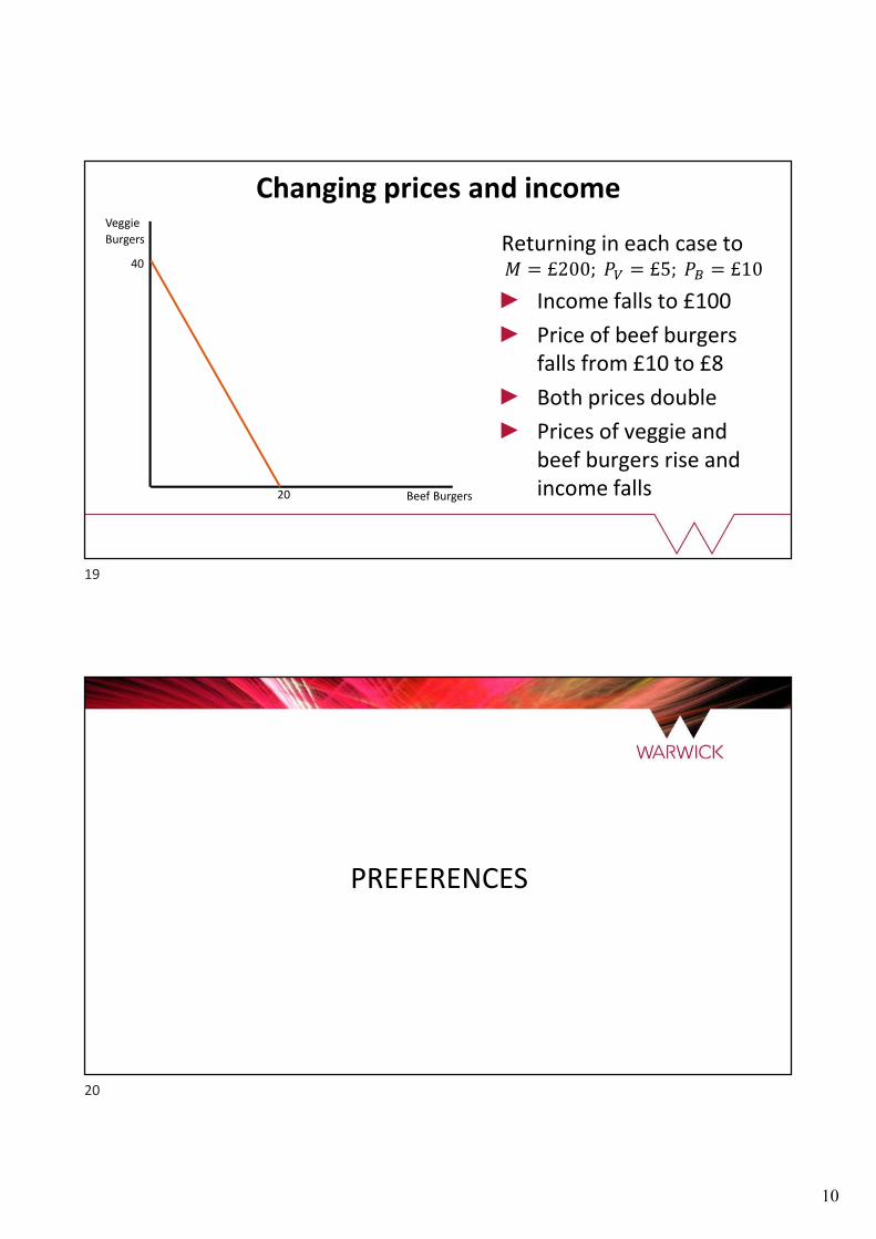
Changing prices and incomeVeggie

Burgers

Beef Burgers

40

20

Returning in each case to� = £200; �� = £5; �� = £10

Income falls to £100

Price of beef burgers falls from £10 to £8

Both prices double

Prices of veggie and beef burgers rise and income falls

PREFERENCES

19

20

11

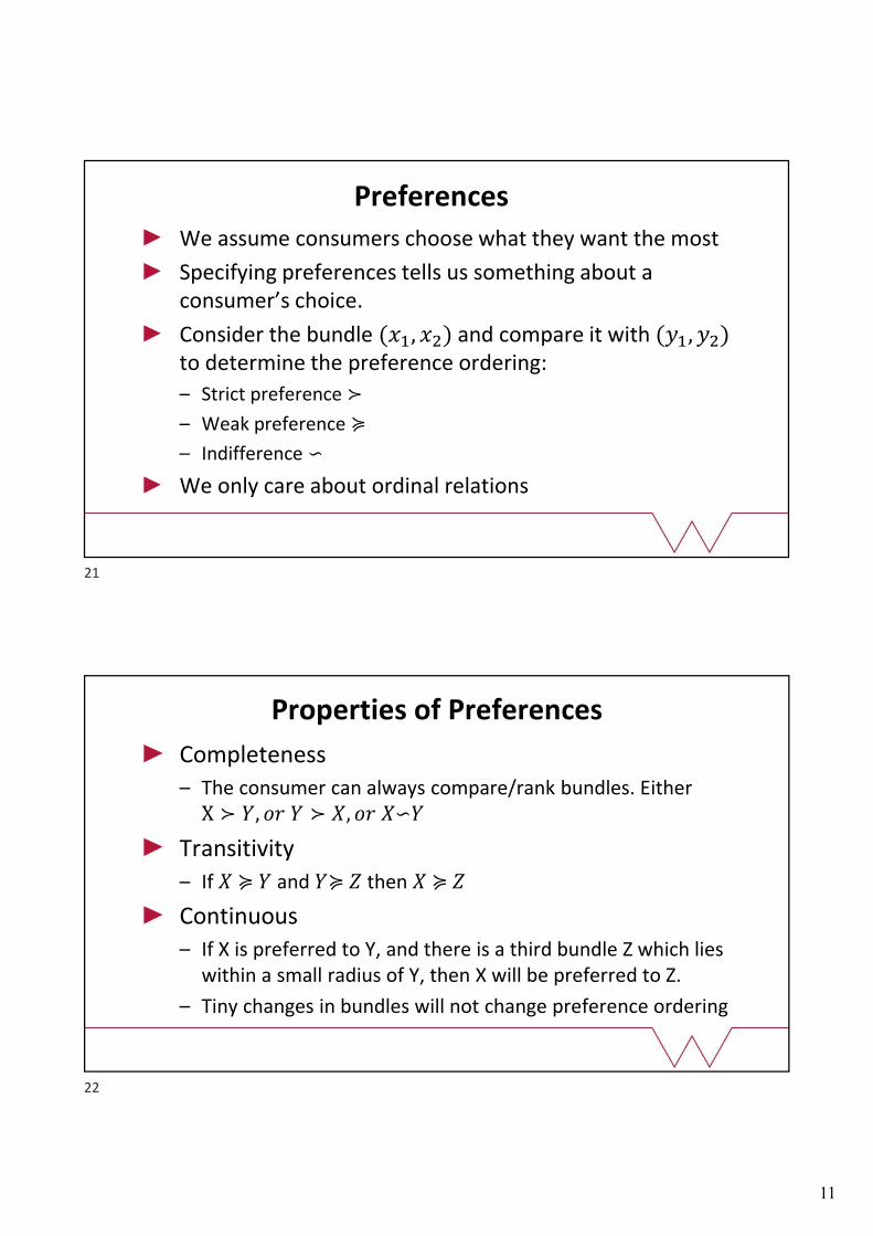
Preferences

We assume consumers choose what they want the most

Specifying preferences tells us something about a consumer’s choice.

Consider the bundle (��, ��) and compare it with (��, ��)to determine the preference ordering:

– Strict preference ≻

– Weak preference ≽

– Indifference ∽

We only care about ordinal relations

Properties of Preferences

Completeness

– The consumer can always compare/rank bundles. Either X ≻ �, �� � ≻ �, �� �∽�

Transitivity

– If � ≽ � and �≽ � then � ≽ �

Continuous

– If X is preferred to Y, and there is a third bundle Z which lies within a small radius of Y, then X will be preferred to Z.

– Tiny changes in bundles will not change preference ordering

21

22

12

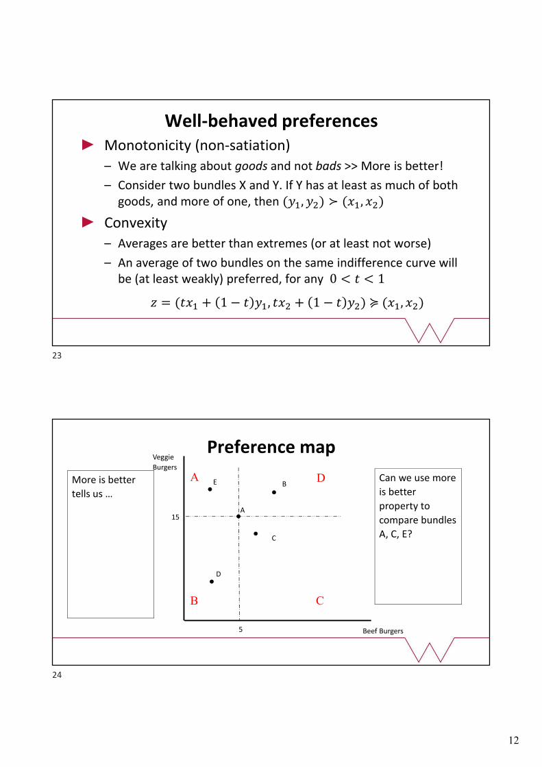
Well-behaved preferencesMonotonicity (non-satiation)

– We are talking about goods and not bads >> More is better!

– Consider two bundles X and Y. If Y has at least as much of both goods, and more of one, then (��, ��) ≻ (��, ��)

Convexity

– Averages are better than extremes (or at least not worse)

– An average of two bundles on the same indifference curve will be (at least weakly) preferred, for any 0 < � < 1

� = (��� + 1 − � ��, ��� + 1 − � ��) ≽ (��, ��)

Preference map

More is better

tells us …

Veggie

Burgers

Beef Burgers

A

B

D

C

5

15

A

B C

DE Can we use more

is better

property to

compare bundles

A, C, E?

23

24

13

Indifference curves IVeggie

Burgers

Beef Burgers

A

E

D

C

5

15

Which bundles do

you like equally to

bundle A?

Connecting these

points (bundles A, C

and E) creates an

indifference curve.

Plotting other

indifference curves

creates an

indifference map.

B

Indifference Curves IIVeggie

Burgers

Beef Burgers

I1

I2

I3

Bundles on I3 are preferred to bundles on I2 etc.

Indifference curves are continuous

Indifference curves cannot cross

Most people’s indifference curves are convex to the origin

Indifference curves are downward sloping

25

26

14

Indifference curves III

Perfect Substitutes – goods with a constant rate of substitution

Perfect Complements – goods that are always consumed together

‘Bads’ – a good that you dislike

Neutral goods – a good that you don’t care about

Satiation – an overall best bundle: too much AND too little is worse

Utility I

Utility Functions describe preferences, assigning higher numbers to more-preferred bundles– All combinations of two goods that give an individual the same

level of utility lie on the same indifference curve

The further from the origin, the higher the utility

Bundle ��, �� ≻ ��, �� iff �(��, ��) ≻ �(��, ��)

We are interested in ordinal and not cardinal utility– We care about which bundle is preferred and not by how much

27

28

15

Utility IIWhat will the utility functions look like for …

Perfect Substitutes:

Perfect Complements:

Cobb-Douglas

– Between the two extremes: Imperfect Substitutes

– The simplest example of well-behaved preferences

– � ��, �� = ���� (or � ��, �� = ��2��

2 )

– � ��, �� = ��

�

���

�

�

– More generally: � ��, �� = ����2

���

Monotonic transformations

Applying monotonic transformations to a utility function creates a new function but with the same preferences– Transforms a set of numbers into another set; preserving the order

– We can’t work back from optimal demands for exact utility function

Consider a utility function �(��, ��, … , ��). Some examples of monotonic transformations:

– log (� ��, ��, … , �� ) − exp � ��, ��, … , ��

– � ��, ��, … , �� + � − �(�(��, ��, … , ��))

– � ��, ��, … , ��n − � ��, ��, … , ��

29

30

16

Behavioural insights IWhich factors affect utility?

Psychological attitudes

Peer group pressures

Personal experiences

The general cultural environment

Ceteris paribus

Only consider choices among quantifiable options

Hold constant other things that affect behaviour

31

32

17

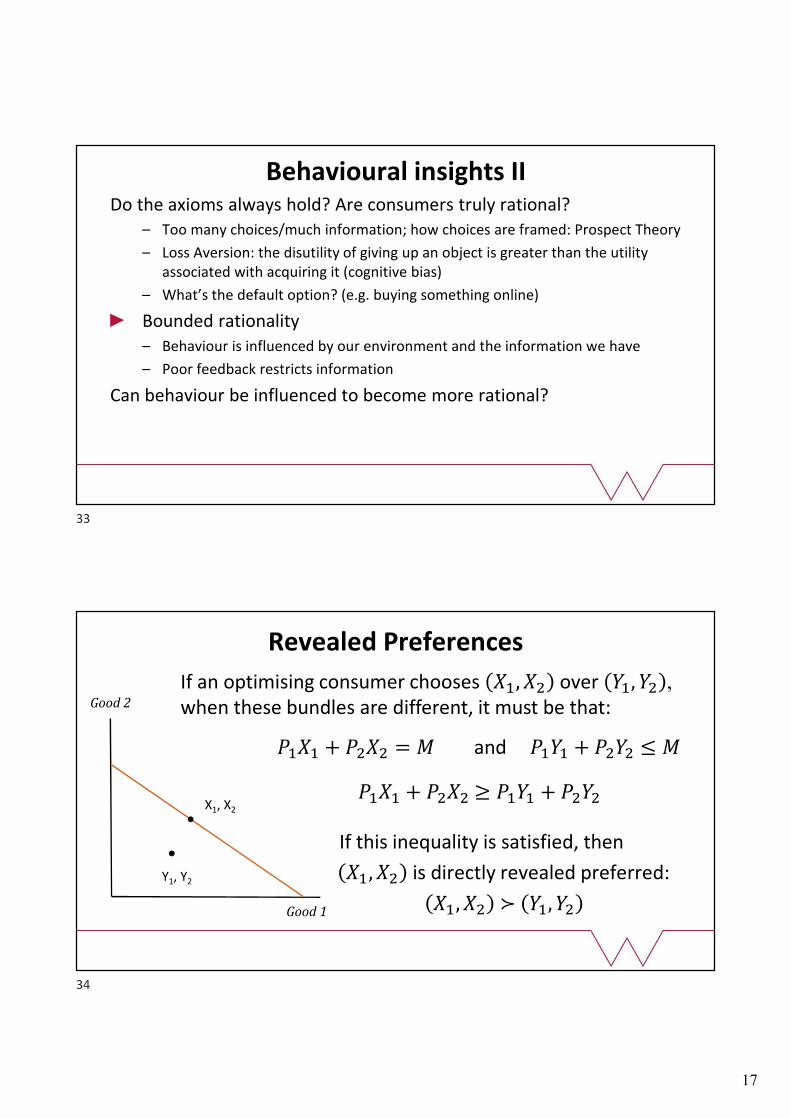
Do the axioms always hold? Are consumers truly rational?– Too many choices/much information; how choices are framed: Prospect Theory

– Loss Aversion: the disutility of giving up an object is greater than the utility associated with acquiring it (cognitive bias)

– What’s the default option? (e.g. buying something online)

Bounded rationality– Behaviour is influenced by our environment and the information we have

– Poor feedback restricts information

Can behaviour be influenced to become more rational?

Behavioural insights II

Good 1

Y1, Y2

X1, X2

Revealed Preferences

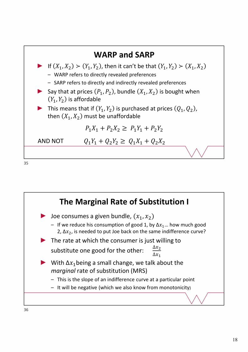
���� + ���� = � and ���� + ���� ≤ �

���� + ���� ≥ ���� + ����

If this inequality is satisfied, then

��, �� is directly revealed preferred:

��, �� ≻ ��, ��

Good 2

If an optimising consumer chooses ��, �� over ��, �� , when these bundles are different, it must be that:

33

34

18

WARP and SARPIf ��, �� ≻ ��, �� , then it can’t be that ��, �� ≻ ��, ��

– WARP refers to directly revealed preferences

– SARP refers to directly and indirectly revealed preferences

Say that at prices ��, �� , bundle ��, �� is bought when ��, �� is affordable

This means that if ��, �� is purchased at prices ��, �� , then ��, �� must be unaffordable

���� + ���� ≥ ���� + ����

AND NOT ���� + ���� ≥ ���� + ����

The Marginal Rate of Substitution I

Joe consumes a given bundle, (��, ��)– If we reduce his consumption of good 1, by ∆��… how much good

2, ∆��, is needed to put Joe back on the same indifference curve?

The rate at which the consumer is just willing to

substitute one good for the other: ∆��

∆��

With ∆��being a small change, we talk about the marginal rate of substitution (MRS)– This is the slope of an indifference curve at a particular point

– It will be negative (which we also know from monotonicity)

35

36

19

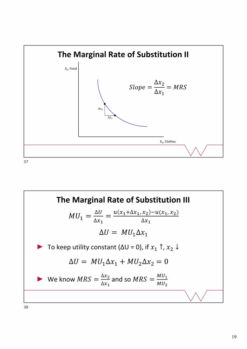
The Marginal Rate of Substitution II

X2, Food

X1, Clothes

∆x2

∆x1

����� =∆��

∆��= ���

��� =∆�

∆��=

� ���∆��, �� ��(��, ��)

∆��

∆� = ���∆��

To keep utility constant (∆U = 0), if �� ↑, �� ↓

∆� = ���∆�� + ���∆�� = 0

We know ��� =∆��

∆��and so ��� =

���

���

The Marginal Rate of Substitution III

37

38

20

We refer to small changes in ��and �� and so

�� = ��(��, ��)

������ +

��(��, ��)

������ = 0

���

���=

�� ��, �����

�� ��, �����

= MRS

The Marginal Rate of Substitution IV

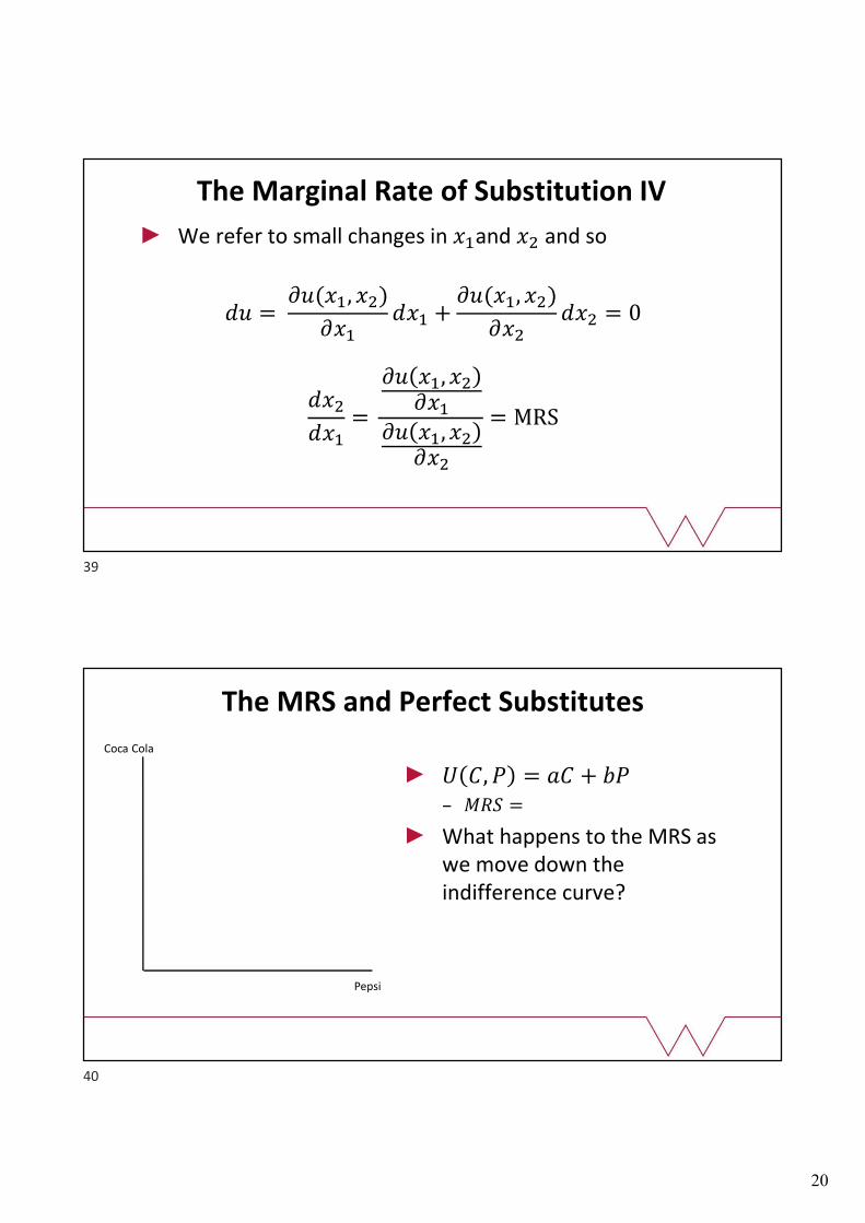
The MRS and Perfect Substitutes

� �, � = �� + ��– ��� =

What happens to the MRS as we move down the indifference curve?

Coca Cola

Pepsi

39

40

21

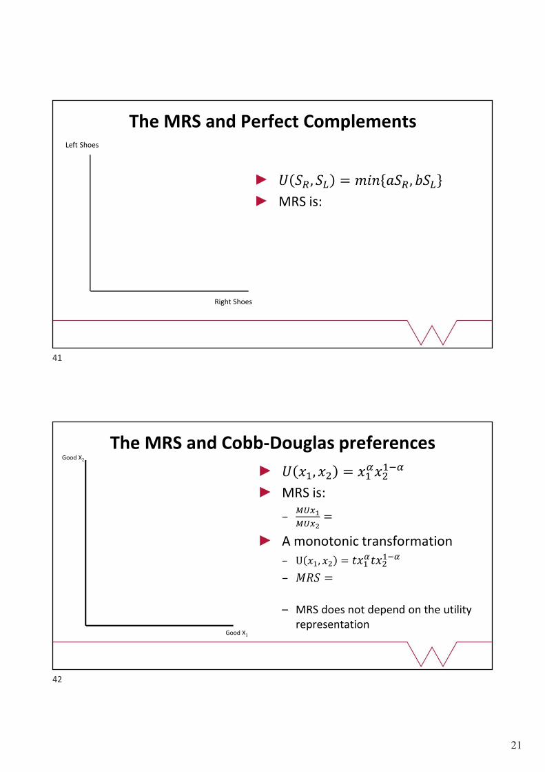
The MRS and Perfect Complements

� ��, �� = ��� ���, ���

MRS is:

Left Shoes

Right Shoes

The MRS and Cobb-Douglas preferencesGood X2

Good X1

� ��, �� = �����

���

MRS is:

–����

����=

A monotonic transformation– U ��, �� = ���

�������

– ��� =

– MRS does not depend on the utility representation

41

42

22

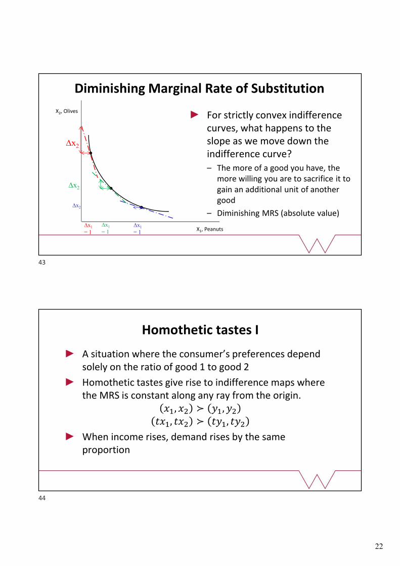
Diminishing Marginal Rate of Substitution

X2, Olives

X1, Peanuts∆x1

= 1

For strictly convex indifference curves, what happens to the slope as we move down the indifference curve?– The more of a good you have, the

more willing you are to sacrifice it to gain an additional unit of another good

– Diminishing MRS (absolute value)∆x1

= 1

∆x2

∆x2

∆x2

∆x1

= 1

Homothetic tastes I

A situation where the consumer’s preferences depend solely on the ratio of good 1 to good 2

Homothetic tastes give rise to indifference maps where the MRS is constant along any ray from the origin.

��, �� ≻ ��, ��

���, ��� ≻ ���, ���

When income rises, demand rises by the same proportion

43

44

23

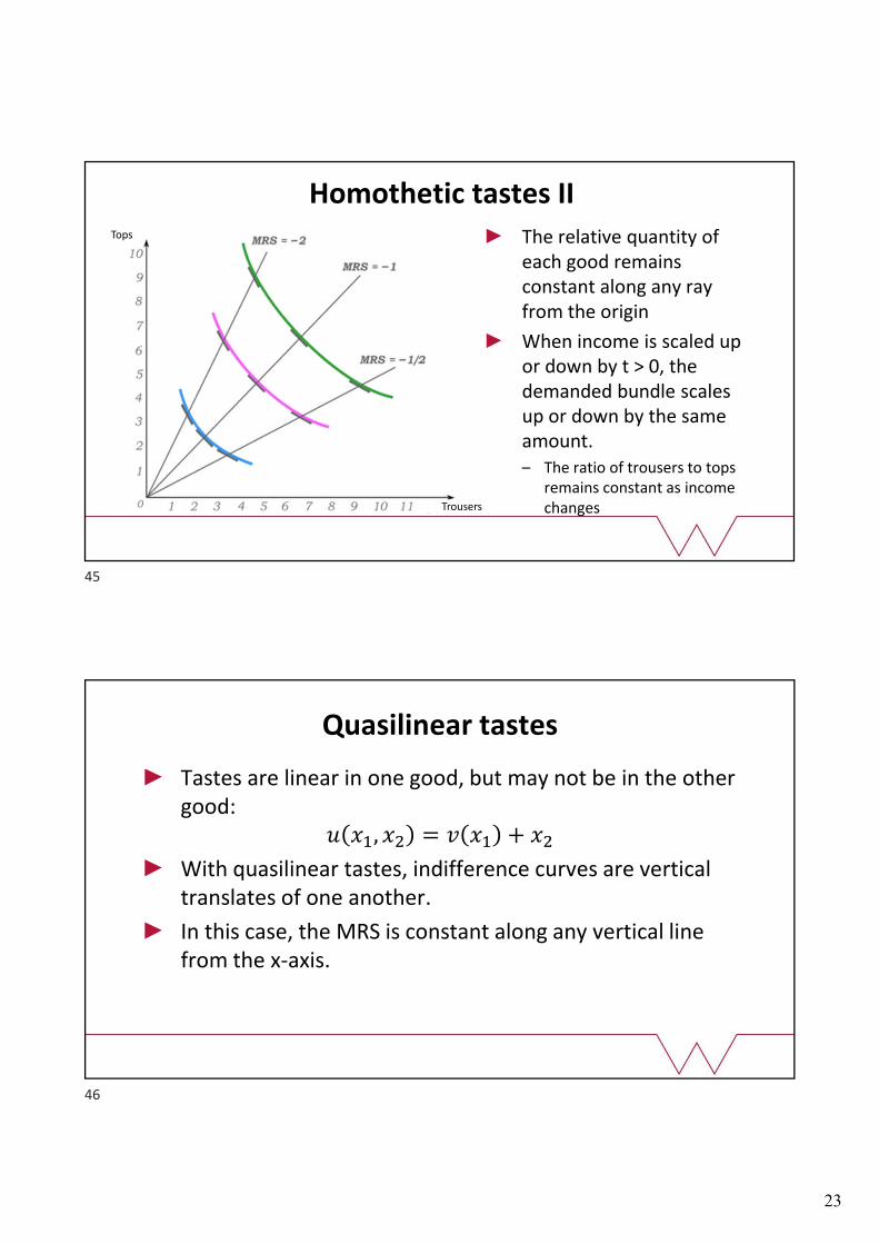
Homothetic tastes II

The relative quantity of each good remains constant along any ray from the origin

When income is scaled up or down by t > 0, the demanded bundle scales up or down by the same amount.– The ratio of trousers to tops

remains constant as income changesTrousers

Tops

Quasilinear tastes

Tastes are linear in one good, but may not be in the other good:

� ��, �� = � �� + ��

With quasilinear tastes, indifference curves are vertical translates of one another.

In this case, the MRS is constant along any vertical line from the x-axis.

45

46

24

Coke and all other consumption

At A, MRS = -1: we will trade $1 for 1 can of coke.

At B, will we value the 50th can of coke the same as the 25th?

– More likely that the 25th

can is valued the same regardless of how much in other consumption we undertake

Elasticity of Substitution IHow does the consumer substitute between �� and ��?

The degree of substitutability measures how responsive the bundle of goods along an IC is to changes in the MRS

The elasticity of substitution is defined as:

– Perfect substitutes: perfect substitutability: σ = ∞

– Perfect complements: no substitutability: σ = 0

– Cobb-Douglas: σ = 1

47

48

25

Elasticity of Substitution II��

��= 10/2

��

��= 4/8

��

��= 10/2

��

��= 8/4

From A to B, there is a large %∆ in x2/x1

From A to B, there is a smaller %∆ in x2/x1

Elasticity of Substitution III

Consider a 1% change in the MRS

The less curved the IC, the more x2 has to fall and the more x1 has to increase for the MRS to have changed by 1%

Thus, the less curvature in the IC, the greater is the % ∆x2/x1 required for the MRS to change by 1%, which implies a higher elasticity of substitution σ– i.e. Perfect Substitutes

49

50

26

OPTIMISATION

Optimisation IGood Y

M/Px

Consumers choose the best bundle within their feasible set

Remember

Slope of budget constraint: ��

��

=Slope of indifference curve:

MRS =���

���

Good X

M/Py

51

52

27

Optimisation II

Consumers maximise utility subject to a budget constraint

This occurs at a tangency, where

��� =��(�, �) ��⁄

��(�, �) ��⁄=

���

���=

��

��

Why must this hold for an interior solution?

– Assume two goods X and Y

– What would happen if:���

���≠

��

��?

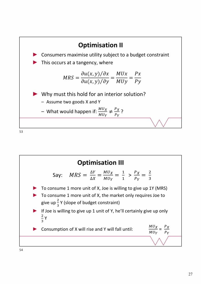
Optimisation III

Say: ��� = ∆�

∆�=

���

���=

�

�>

��

��=

�

�

To consume 1 more unit of X, Joe is willing to give up 1Y (MRS)

To consume 1 more unit of X, the market only requires Joe to

give up �

�Y (slope of budget constraint)

If Joe is willing to give up 1 unit of Y, he’ll certainly give up only �

�Y

Consumption of X will rise and Y will fall until: ���

���=

��

��

53

54

28

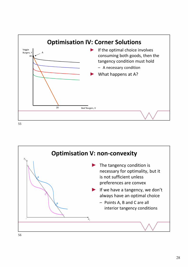
Optimisation IV: Corner Solutions

40

20

If the optimal choice involves consuming both goods, then the tangency condition must hold

– A necessary condition

What happens at A?

AVeggie

Burgers, Y

Beef Burgers, X

Optimisation V: non-convexity

The tangency condition is necessary for optimality, but it is not sufficient unless preferences are convex

If we have a tangency, we don’t always have an optimal choice

– Points A, B and C are all interior tangency conditions

55

56

29

Equi-marginal Principle I

We can find the optimum bundle by setting the MRS equal to the price ratio and using the budget constraint.

The solutions give the Marshallian demands – demand is dependent on prices and income: �∗ ��, ��, �

An example: � = �����

���, with ��, ��, �

Find the MRS and set equal to the price ratio: ��

��=

��

��

Rearrange to give (say): ���� = ����

Plug into the budget constraint

Equi-marginal Principle II

� = ���� + ���� But ���� = ����

� = ���� + ���� >> � = 2����

So, we can find: �� =�

���

Plug the demand for �� into the budget constraint:

� = ���

���+ ���� >> 2� = � + 2����

�� =����

���=

�

���

Demand is dependent on prices and income

57

58

30

Marshallian demands I

What if we have a utility function where there isn’t a tangency?

Perfect Substitutes

Perfect Complements– In each case, think about it logically…

– In the diagram, what do we know about how consumers will allocate their income?

– What do we know about the point at which consumers maximise their utility?

Marshallian demands II

Perfect Substitutes:

��∗ = �

�/��

0 < 0

��∗ < �/��

Coca Cola

Pepsi

Budget Constraint

�� �� < ��

�� �� = ��

�� �� > ��

Maximise utility on highest IC subject to BC:

Compare slopes of BC and IC to determine which good is consumed

59

60

31

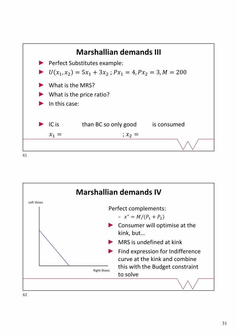
Marshallian demands IIIPerfect Substitutes example:

� ��, �� = 5�� + 3�� ; ��� = 4, ��� = 3, � = 200

What is the MRS?

What is the price ratio?

In this case:

IC is than BC so only good is consumed

�� = ; �� =

Marshallian demands IV

Perfect complements:– �∗ = �/(�� + ��)

Consumer will optimise at the kink, but…

MRS is undefined at kink

Find expression for Indifference curve at the kink and combine this with the Budget constraint to solve

Left Shoes

Right Shoes

61

62

32

Marshallian demands VPerfect Complements example:

� ��, �� = min {4��, 3��} ; ��� = 4, ��� = 3, � = 200

How many units of �� ��� �� do we have at the kink?

(1)

Find an expression for the BC. (2)

Substitute (1) into (2):

Solve: �� = ; �� =

Marshallian demands VICobb-Douglas: � = ��

����

��∗ =

�

���

�

��and ��

∗ =�

���

�

��

It is convenient to write Cobb-Douglas utility functions with exponents that sum to 1

– Raise utility to power 1 � + �⁄ ≫ � = �����

���

A fixed proportion of income is spent on each good– The size is determined by the exponents, e.g. good 1 = α

– Marshallian demand: ��∗ =

��

��and ��

∗ =(���)�

��

63

64

33

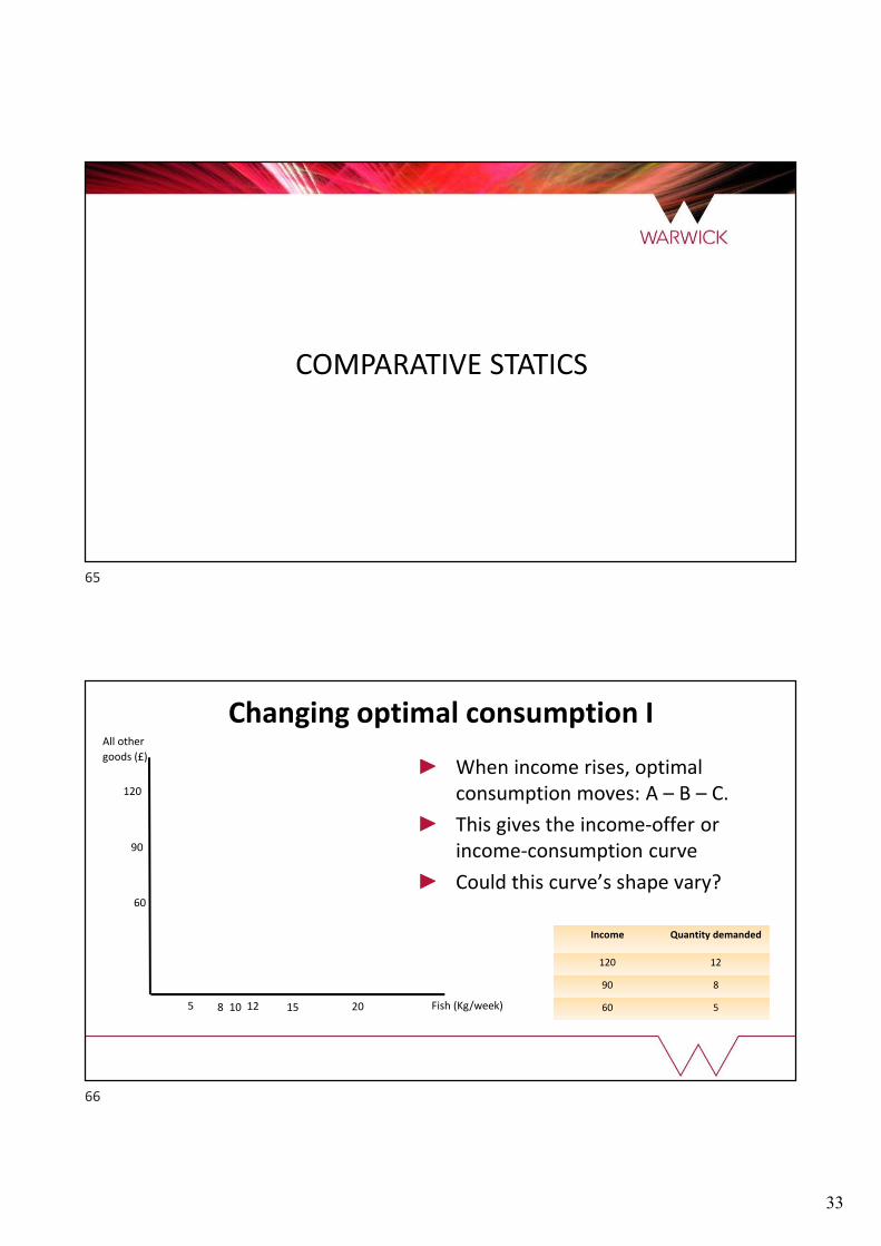
COMPARATIVE STATICS

When income rises, optimal consumption moves: A – B – C.

This gives the income-offer or income-consumption curve

Could this curve’s shape vary?

Changing optimal consumption IAll other

goods (£)

Fish (Kg/week)

60

90

120

5 8 1210 15 20

Income Quantity demanded

120 12

90 8

60 5

65

66

34

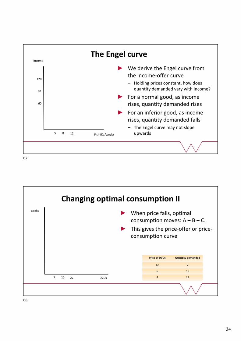
The Engel curve Income

Fish (Kg/week)

60

90

120

5 8 12

We derive the Engel curve from the income-offer curve– Holding prices constant, how does

quantity demanded vary with income?

For a normal good, as income rises, quantity demanded rises

For an inferior good, as income rises, quantity demanded falls– The Engel curve may not slope

upwards

Changing optimal consumption II Books

DVDs

Price of DVDs Quantity demanded

12 7

6 15

4 22

When price falls, optimal consumption moves: A – B – C.

This gives the price-offer or price-consumption curve

7 15 22

67

68

35

The Demand Curve IPrice (P)

DVDs

Quantity

demanded, DVDs

12

6

4

7 15 22

We derive the demand curve for DVDs from the price-offer curve– Holding income, other prices

and preferences constant, how does quantity demanded change following a price change?

– What happens to demand if income, other prices or preferences change?

The Demand Curve II

The law of demand

The substitution effect: As �� ↓, good Y becomes relatively more expensive and less attractive to the consumer.

Even remaining on the same IC, the price ratio changes– Optimal demands will change to where: MRS = NEW price ratio

The income effect: As �� ↓, real income rises. The consumer now feels richer, so quantity demanded changes. – As real income changes, the consumer must move to a new IC

69

70

36

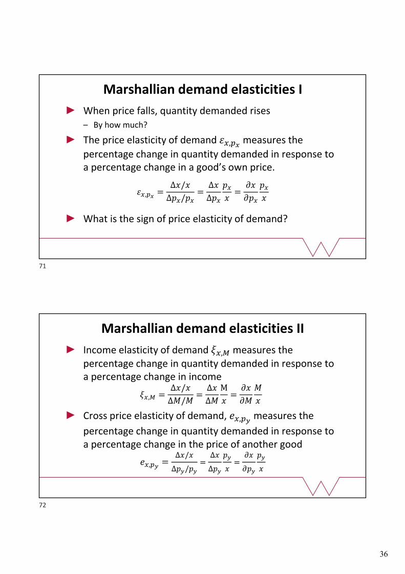
Marshallian demand elasticities I

When price falls, quantity demanded rises– By how much?

The price elasticity of demand ��,��measures the

percentage change in quantity demanded in response to a percentage change in a good’s own price.

��,��=

Δ�/�

��/��=

Δ�

��

��

�=

��

���

��

�

What is the sign of price elasticity of demand?

Marshallian demand elasticities II

Income elasticity of demand ��,� measures the percentage change in quantity demanded in response to a percentage change in income

��,� =�/�

Δ�/�=

Δ�

Δ�

M

�=

��

��

�

�

Cross price elasticity of demand, ��,��measures the

percentage change in quantity demanded in response to a percentage change in the price of another good

��,��=

Δ�/�

��/��

=Δ�

��

��

�=

��

���

��

�

71

72

37

CONSUMER THEORY IN PRACTICE

Income and substitution effects

Two goods: apples and bananas and price of apples falls

Apples are relatively cheaper (substitution effect), so the consumer can afford to buy more (income effect)– How many more are bought just because they are cheaper?

– What’s the change in demand ONLY due to the substitution effect?

Graphical analysis: what we do– When price falls (BC pivots), real income rises … but ignore that by

– … taking some income from the consumer (shift new BC) so that …

73

74

38

Income and substitution effects

Either (1)– Utility is the same after the price change as it was before the price change (that

way the consumer is no better off despite the lower price)

Or (2)– Purchasing power is the same after the price change as it was before the price

change (the consumer has just enough income to buy the original bundle)

(1): Hicksian

(2): Slutsky

Both only consider the substitution effect (the change in demand purely because the good is cheaper)

76

What’s the point?Government is about to introduce an energy tax and is concerned about the impact on pensioners– How much less energy will pensioners consume at this higher price?

Government doesn’t want pensioners worse off - key votes!– By how much should their pension rise so they are no worse off?

As a government economist, you will be asked to find:– The change in demand due to the substitution effect

– Original welfare of pensioners, to calculate required ‘compensation’

– Then it’s interesting to see how energy consumption has changed with the tax and the increased pension payments

75

76

39

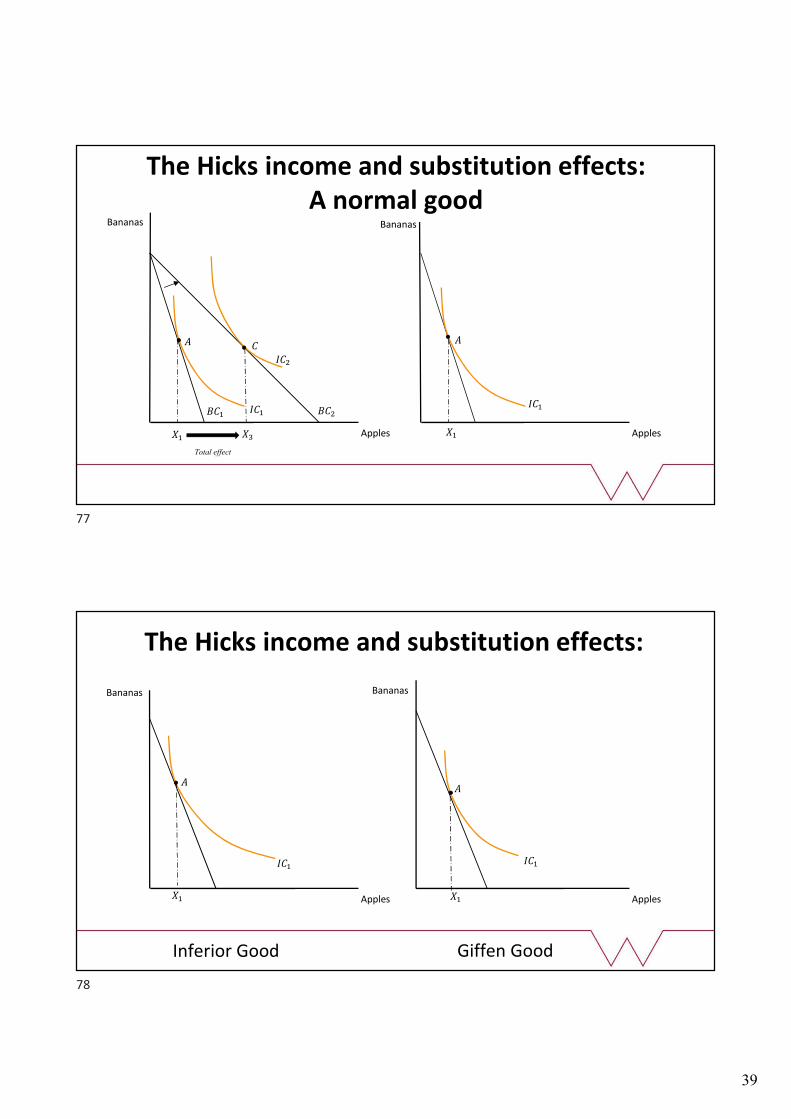
The Hicks income and substitution effects:A normal good

Bananas

Apples����

Bananas

Apples��

������

���

���

��� ���

Total effect

The Hicks income and substitution effects:

Bananas

Apples��

Bananas

Apples��

������

��

Inferior Good Giffen Good

77

78

40

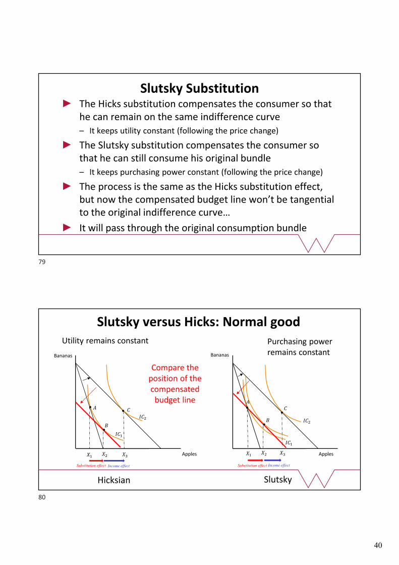
Slutsky SubstitutionThe Hicks substitution compensates the consumer so that he can remain on the same indifference curve– It keeps utility constant (following the price change)

The Slutsky substitution compensates the consumer so that he can still consume his original bundle– It keeps purchasing power constant (following the price change)

The process is the same as the Hicks substitution effect, but now the compensated budget line won’t be tangential to the original indifference curve…

It will pass through the original consumption bundle

Slutsky versus Hicks: Normal good

Bananas

Apples����

Bananas

Apples���� ��

���

���

���

���

�

�

�

��

Income effectSubstitution effect

Compare the position of the compensated

budget line

Utility remains constant

��

�

Hicksian Slutsky

Substitution effect Income effect

Purchasing power remains constant

79

80

41

81

Hicksian: The Dual Problem I

Find the initial bundle (at original price ratio)– Utility maximisation: Consume on highest IC subject to BC

Find the change in demand due to the substitution effect– Expenditure minimisation: what is the least costly way of

achieving the original level of utility at the new price ratio?

Find the new bundle (at new price ratio)– Utility maximisation (now also takes into account the income

effect)

82

Slutsky substitutionFind the change in income needed to make the original bundle affordable at new price, ��

�

Original Income: � = ���� + ����

New Income: �� = ��′�� + ����

∆� = �� − � = ����� − ���� = ��∆��

The change in income tells us the new amount of income the consumer needs such that they can just buy the original bundle at the new set of prices

81

82

42

83

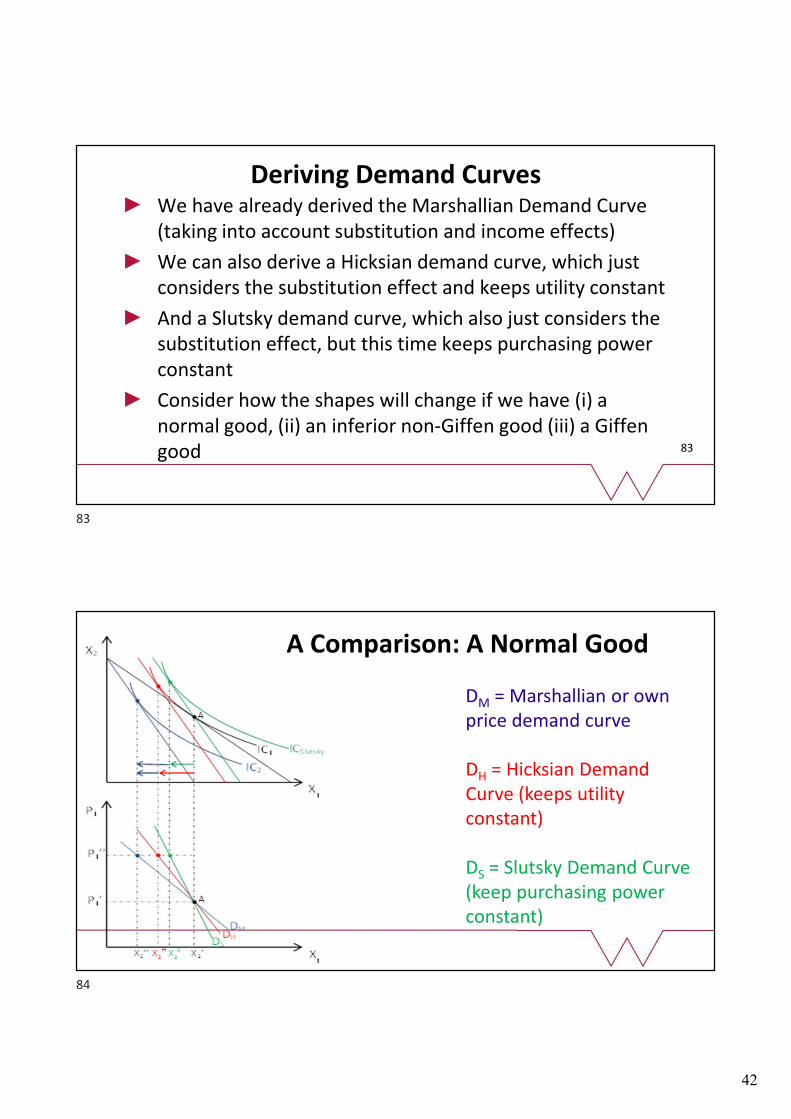
Deriving Demand CurvesWe have already derived the Marshallian Demand Curve (taking into account substitution and income effects)

We can also derive a Hicksian demand curve, which just considers the substitution effect and keeps utility constant

And a Slutsky demand curve, which also just considers the substitution effect, but this time keeps purchasing power constant

Consider how the shapes will change if we have (i) a normal good, (ii) an inferior non-Giffen good (iii) a Giffengood

DM = Marshallian or own price demand curve

DH = Hicksian Demand Curve (keeps utility constant)

DS = Slutsky Demand Curve (keep purchasing power constant)

A Comparison: A Normal Good

83

84

43

OPTIMISING MATHEMATICALLY

Optimising mathematically: The Primal

If we know income, prices and the utility function:

max��,��,λ

� = � ��, �� + λ(� − ���� − ����)

and solve for the Marshallian demands: �∗ ��, ��, �– Demand is homogenous of degree zero

• �∗ ��, ��, � = �∗ ���, ���, �� ��� � > 0

– If utility is monotonic then the budget binds

Tangency is necessary, not sufficient. Only sufficient if preferences are convex– If preferences are not convex, check SOC to ensure a maximum

85

86

44

The Lagrange multiplier

Tangency implies:

λ∗ =���

��=

���

��= ⋯ =

���

��= ⋯ =

���

��

λ∗ is the marginal utility of an extra £ of expenditure– The marginal utility of income

– £1 of extra income will increase utility by λ

Price is the consumer’s evaluation of the utility of the last unit consumed

�� =���

�for every i

88

A reminder: The Dual Problem I

Find the initial bundle (at original price ratio)– Utility maximisation: Consume on highest IC subject to BC

Find the change in demand due to the substitution effect– Expenditure minimisation: what is the least costly way of

achieving the original level of utility at the new price ratio?

Find the new bundle (at new price ratio)– Utility maximisation (now also takes into account the income

effect)

87

88

45

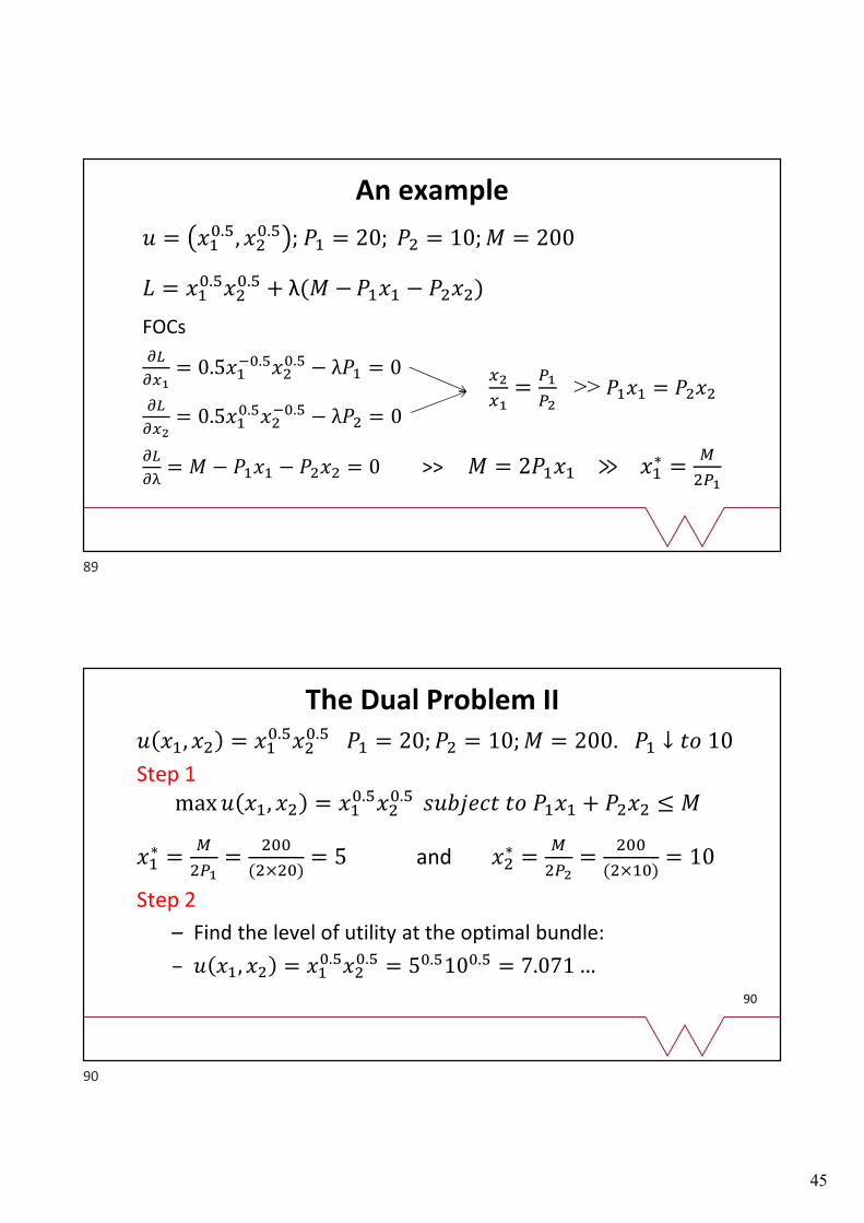
An example

� = ���.�, ��

�.� ; �� = 20; �� = 10; � = 200

� = ���.���

�.� + λ(� − ���� − ����)

FOCs

��

���= 0.5��

��.����.� − λ�� = 0

��

���= 0.5��

�.�����.� − λ�� = 0

��

��= � − ���� − ���� = 0 >> � = 2���� ≫ ��

∗ =�

���

��

��=

��

��>> ���� = ����

90

The Dual Problem II� ��, �� = ��

�.����.� �� = 20; �� = 10; � = 200. �� ↓ �� 10

Step 1max � ��, �� = ��

�.����.� ������� �� ���� + ���� ≤ �

��∗ =

�

���=

���

(���)= 5 and ��

∗ =�

���=

���

(���)= 10

Step 2

– Find the level of utility at the optimal bundle:

– � ��, �� = ���.���

�.� = 5�.�10�.� = 7.071 …

89

90

46

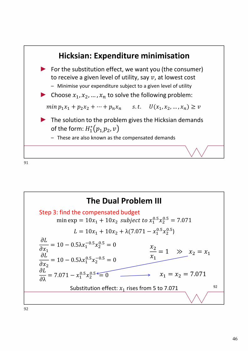
Hicksian: Expenditure minimisation

For the substitution effect, we want you (the consumer) to receive a given level of utility, say �, at lowest cost– Minimise your expenditure subject to a given level of utility

Choose ��, ��, … , �� to solve the following problem:

��� ���� + ���� + ⋯ + ���� �. �. �(��, ��, … , ��) ≥ �

The solution to the problem gives the Hicksian demands

of the form: ��∗ ��,��, �

– These are also known as the compensated demands

92

The Dual Problem IIIStep 3: find the compensated budget

min exp = 10�� + 10�� ������� �� ���.���

�.� = 7.071

� = 10�� + 10�� + λ(7.071 − ���.���

�.�)

��

���= 10 − 0.5λ��

��.����.� = 0

��

���= 10 − 0.5λ��

�.�����.� = 0

��

�λ= 7.071 − ��

�.����.� = 0

Substitution effect: �� rises from 5 to 7.071

��

��= 1 ≫ �� = ��

�� = �� = 7.071

91

92

47

93

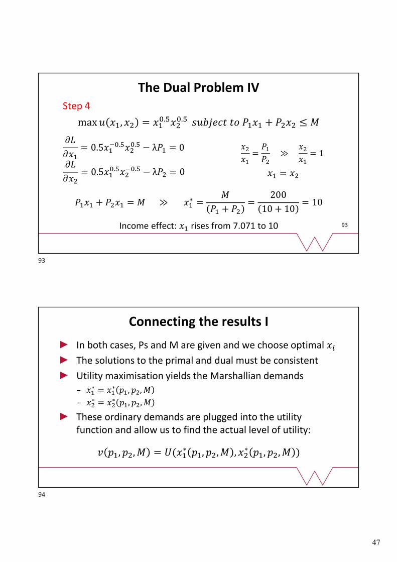
The Dual Problem IVStep 4

max � ��, �� = ���.���

�.� ������� �� ���� + ���� ≤ �

��

���= 0.5��

��.����.� − λ�� = 0

��

���= 0.5��

�.�����.� − λ�� = 0

���� + ���� = � ≫ ��∗ =

�

�� + ��=

200

10 + 10= 10

Income effect: �� rises from 7.071 to 10

��

��=

��

�� ≫

��

��= 1

�� = ��

Connecting the results I

In both cases, Ps and M are given and we choose optimal ��

The solutions to the primal and dual must be consistent

Utility maximisation yields the Marshallian demands

– ��∗ = ��

∗ ��, ��, �

– ��∗ = ��

∗ ��, ��, �

These ordinary demands are plugged into the utility function and allow us to find the actual level of utility:

� ��, ��, � = �(��∗ ��, ��, � , ��

∗ ��, ��, � )

93

94

48

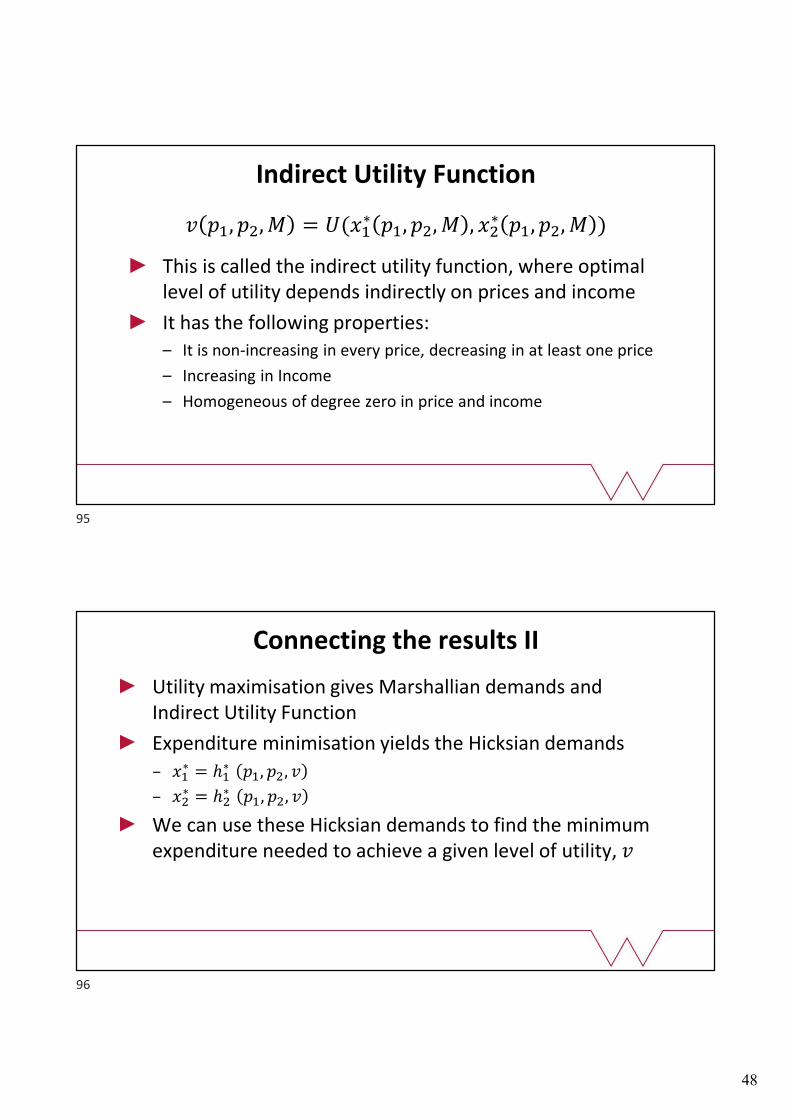
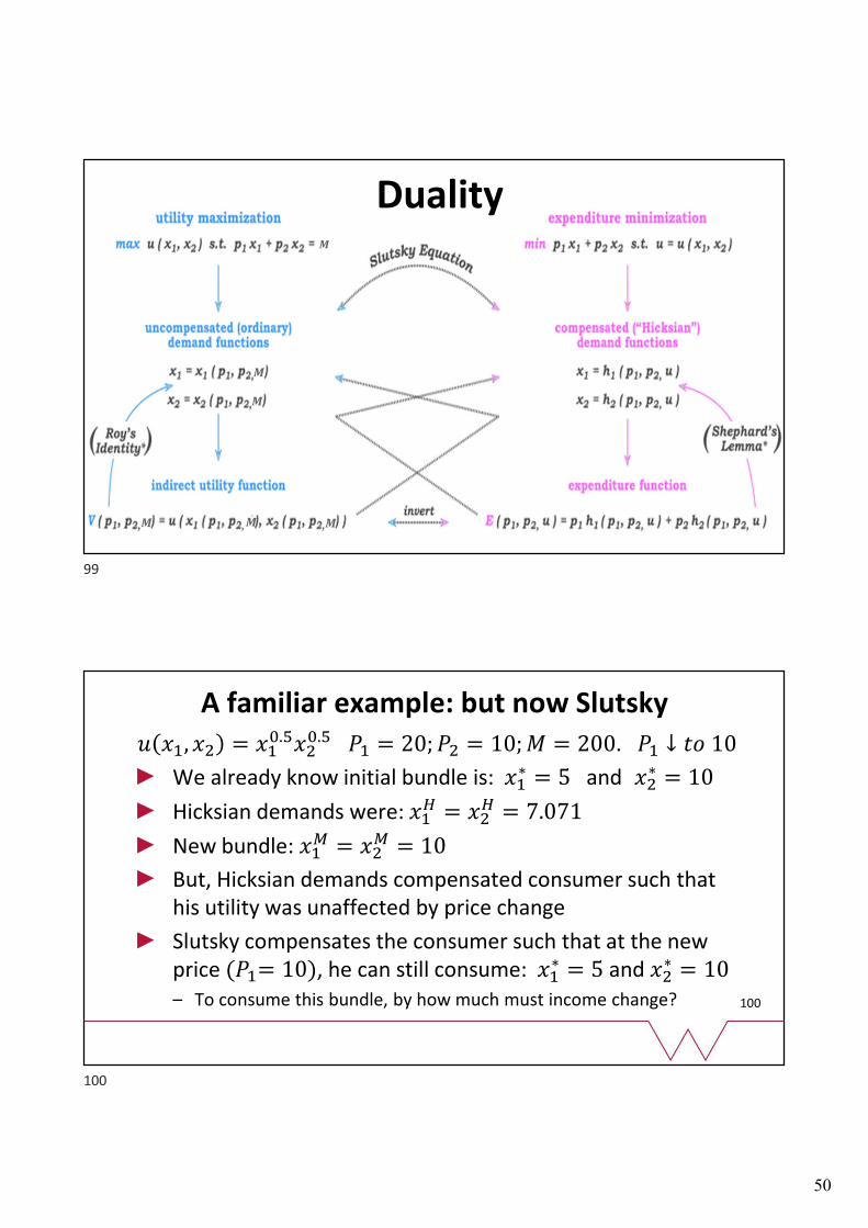
Indirect Utility Function

� ��, ��, � = �(��∗ ��, ��, � , ��

∗ ��, ��, � )

This is called the indirect utility function, where optimal level of utility depends indirectly on prices and income

It has the following properties:– It is non-increasing in every price, decreasing in at least one price

– Increasing in Income

– Homogeneous of degree zero in price and income

Connecting the results II

Utility maximisation gives Marshallian demands and Indirect Utility Function

Expenditure minimisation yields the Hicksian demands

– ��∗ = ℎ�

∗ ��, ��, �

– ��∗ = ℎ�

∗ ��, ��, �

We can use these Hicksian demands to find the minimum expenditure needed to achieve a given level of utility, �

95

96

49

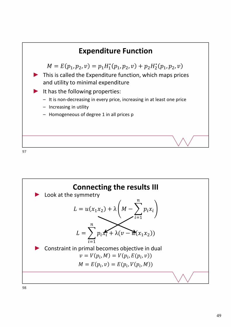
Expenditure Function

� = � ��, ��, � = ����∗ ��, ��, � + ����

∗ ��, ��, �

This is called the Expenditure function, which maps prices and utility to minimal expenditure

It has the following properties:– It is non-decreasing in every price, increasing in at least one price

– Increasing in utility

– Homogeneous of degree 1 in all prices p

Connecting the results III Look at the symmetry

� = � ���� + λ � − � ����

�

���

� = � ����

�

���

+ λ(� − � ���� )

Constraint in primal becomes objective in dual� = � ��, � = � ��, �(��, � )

� = � ��, � = �(��, � ��, � )

97

98

50

Duality�

�

�

� � �

100

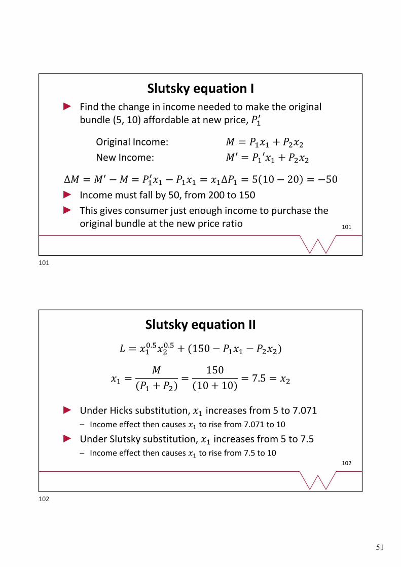
A familiar example: but now Slutsky� ��, �� = ��

�.����.� �� = 20; �� = 10; � = 200. �� ↓ �� 10

We already know initial bundle is: ��∗ = 5 and ��

∗ = 10

Hicksian demands were: ��� = ��

� = 7.071

New bundle: ��� = ��

� = 10

But, Hicksian demands compensated consumer such that his utility was unaffected by price change

Slutsky compensates the consumer such that at the new price (��= 10), he can still consume: ��

∗ = 5 and ��∗ = 10

– To consume this bundle, by how much must income change?

99

100

51

101

Slutsky equation IFind the change in income needed to make the original bundle (5, 10) affordable at new price, ��

�

Original Income: � = ���� + ����

New Income: �� = ��′�� + ����

∆� = �� − � = ����� − ���� = ��∆�� = 5 10 − 20 = −50

Income must fall by 50, from 200 to 150

This gives consumer just enough income to purchase the original bundle at the new price ratio

102

Slutsky equation II

� = ���.���

�.� + (150 − ���� − ����)

�� =�

(�� + ��)=

150

(10 + 10)= 7.5 = ��

Under Hicks substitution, �� increases from 5 to 7.071– Income effect then causes �� to rise from 7.071 to 10

Under Slutsky substitution, �� increases from 5 to 7.5 – Income effect then causes �� to rise from 7.5 to 10

101

102

52

103

Slutsky equation III

Substitution effect: ∆��� = �� ��

�, �� − �� ��, �

Income effect: ∆��� = �� ��

�, � − �� ��′, �′

Total effect: ∆�� = �� ���, � − �� ��, � = ∆��

� + ∆���

Express as rates of change by defining ∆��� as −∆��

�

∆�� = ∆��� − ∆��

�

Divide each side by ∆��∆��

∆��=

∆���

∆��−

∆���

∆��

104

Slutsky equation IV∆��

∆��=

∆���

∆��−

∆���

∆��and recall: ∆� = ��∆�� >> ∆�� =

∆�

��

Replace denominator in term 3∆��

∆��=

∆���

∆��−

∆���

∆���

1. Rate of change of �� following a change in ��, holding M fixed (total effect)

2. Rate of change of �� as �� changes, adjusting M to keep old bundle affordable (substitution effect)

3. Rate of change of ��, holding prices fixed and adjusting M (income effect)

103

104

53

WELFARE

A change in welfare IIn policy debates it is important to be able to quantify how consumer “welfare” is affected by changing prices.– How is welfare affected if fuel tax rises, or a carbon tax is introduced?

– A key part of economists’ role in government, regulators, consulting

We can’t look at utility directly (ordinal utility), so we use a proxy – income or money

There are 3 ways that changes in welfare can be measured– Consumer Surplus

– Compensating variation

– Equivalent variation

105

106

54

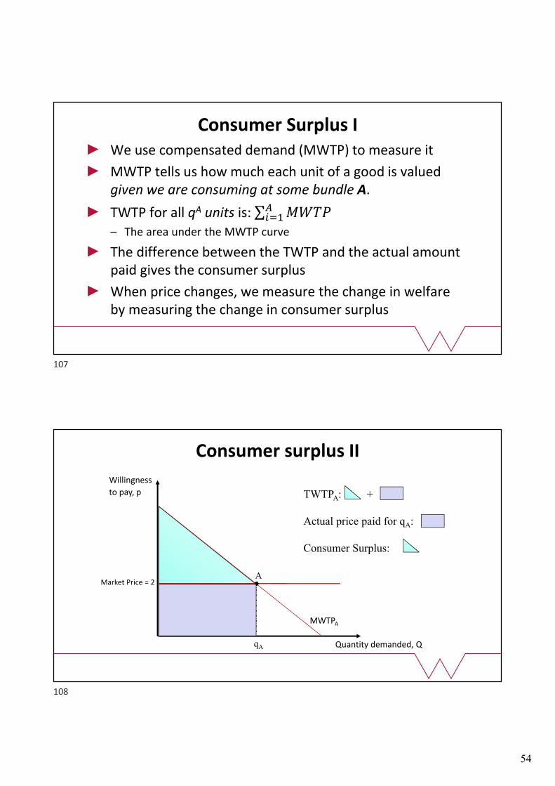
Consumer Surplus IWe use compensated demand (MWTP) to measure it

MWTP tells us how much each unit of a good is valued given we are consuming at some bundle A.

TWTP for all qA units is: ∑ ��������

– The area under the MWTP curve

The difference between the TWTP and the actual amount paid gives the consumer surplus

When price changes, we measure the change in welfare by measuring the change in consumer surplus

Consumer surplus II

Willingness

to pay, p

Quantity demanded, Q

Market Price = 2

TWTPA: +

Actual price paid for qA:

Consumer Surplus:

MWTPA

A

qA

107

108

55

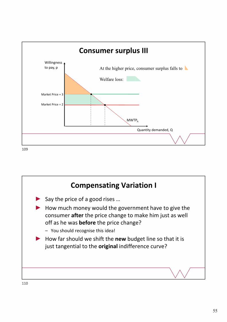
Consumer surplus III

Willingness

to pay, p

Quantity demanded, Q

Market Price = 2

At the higher price, consumer surplus falls to

Welfare loss:

Market Price = 3

MWTPA

Compensating Variation I

Say the price of a good rises …

How much money would the government have to give the consumer after the price change to make him just as well off as he was before the price change?– You should recognise this idea!

How far should we shift the new budget line so that it is just tangential to the original indifference curve?

109

110

56

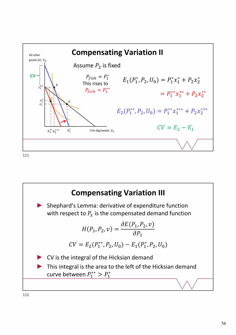
Compensating Variation IIAll other

goods (£): ��

Fish (Kg/week): ��

�

��

��∗∗

����� = ��∗

This rises to����� = ��

∗∗

��(��∗, ��, ��) = ��

∗��∗ + ����

∗

��∗∗∗ ��

∗

��∗∗

��∗

��∗∗∗

= ��∗∗��

∗∗ + ����∗∗

��(��∗∗, ��, ��) = ��

∗∗��∗∗∗ + ����

∗∗∗

�� = �� − ��

Assume �� is fixed

CV

Compensating Variation III

Shephard’s Lemma: derivative of expenditure function with respect to �� is the compensated demand function

� ��, ��, � =��(��, ��, �)

���

�� = ��(��∗∗, ��, ��) − ��(��

∗, ��, ��)

CV is the integral of the Hicksian demand

This integral is the area to the left of the Hicksian demand curve between ��

∗∗ > ��∗

111

112

57

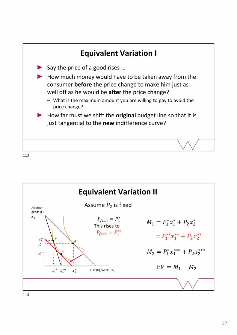
Equivalent Variation I

Say the price of a good rises …

How much money would have to be taken away from the consumer before the price change to make him just as well off as he would be after the price change?– What is the maximum amount you are willing to pay to avoid the

price change?

How far must we shift the original budget line so that it is just tangential to the new indifference curve?

Equivalent Variation II

All other

goods (£):

��

Fish (Kg/week): ��

�

��

��∗∗

����� = ��∗

This rises to����� = ��

∗∗

�� = ��∗��

∗ + ����∗

��∗∗∗ ��

∗

��∗∗∗

��∗

��∗∗

= ��∗∗��

∗∗ + ����∗∗

�� = ��∗��

∗∗∗ + ����∗∗∗

E� = �� − ��

Assume �� is fixed

113

114

58

Consumer surplus, compensating variation and equivalent variation can give different values– The same change in price can lead to different changes in welfare,

depending on how we measure it

£1 is worth differing amounts at different prices

CS, CV and EV will only be equal to each other if tastes are quasilinear– As here, there is no income effect

A change in welfare II

APPLICATIONS

115

116

59

Endowments of goods IAn endowment: A bundle of goods owned by a consumer and tradable for other goods:(��, ��)

Say you have �� of good 1, but would choose �� > ��

– This means you are a net demander/buyer of good 1

– If you would choose �� < ��, you are a net supplier/seller of good 1

Income is determined by your endowments and prices

Consumer’s choice set depends on endowments and prices

� ��, ��, ��, �� = ��, �� |���� + ���� ≤ ���� + ����

The budget constraint will always pass through (��, ��)

Endowments of goods IISay you bought 5 pairs of jeans �� at £20 each and 10 jumpers (��) at £10 each from John Lewis for your partner– But they say that you bought the wrong ones and wrong quantities!

You return to John Lewis, but don’t have the receipt– You get a Gift Certificate for your goods at the current prices

– � = 5�� + 10��

If prices are unchanged, budget constraint is unchanged

If prices have changed, budget constraint must still pass through (��, ��) but will now have a different slope and intercepts

117

118

60

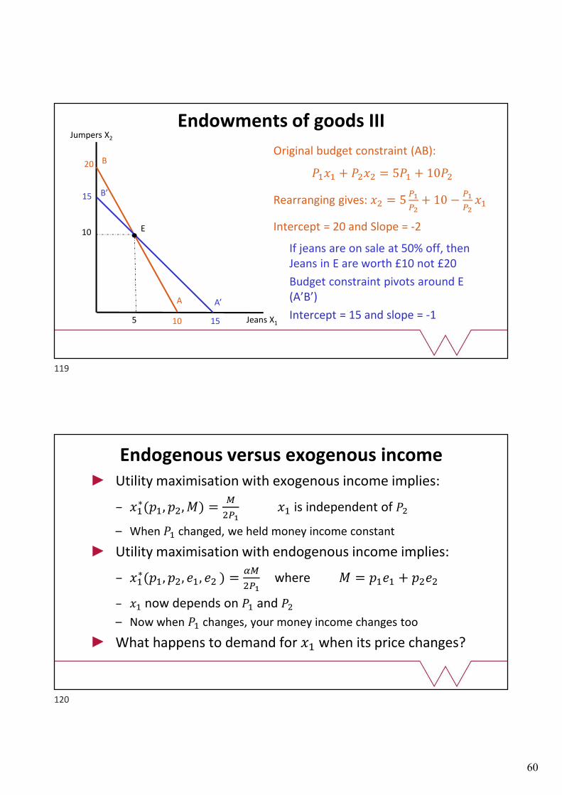
Endowments of goods III

Original budget constraint (AB):

���� + ���� = 5�� + 10��

Rearranging gives: �� = 5��

��+ 10 −

��

����

Intercept = 20 and Slope = -2

20

5

10

Jumpers X2

Jeans X1

E

15

10 15

A

B

A’

B’

If jeans are on sale at 50% off, then Jeans in E are worth £10 not £20

Budget constraint pivots around E (A’B’)

Intercept = 15 and slope = -1

Endogenous versus exogenous incomeUtility maximisation with exogenous income implies:

– ��∗(��, ��, �) =

�

����� is independent of ��

– When �� changed, we held money income constant

Utility maximisation with endogenous income implies:

– ��∗(��, ��, ��, �� ) =

��

���where � = ���� + ����

– �� now depends on �� and ��

– Now when �� changes, your money income changes too

What happens to demand for �� when its price changes?

119

120

61

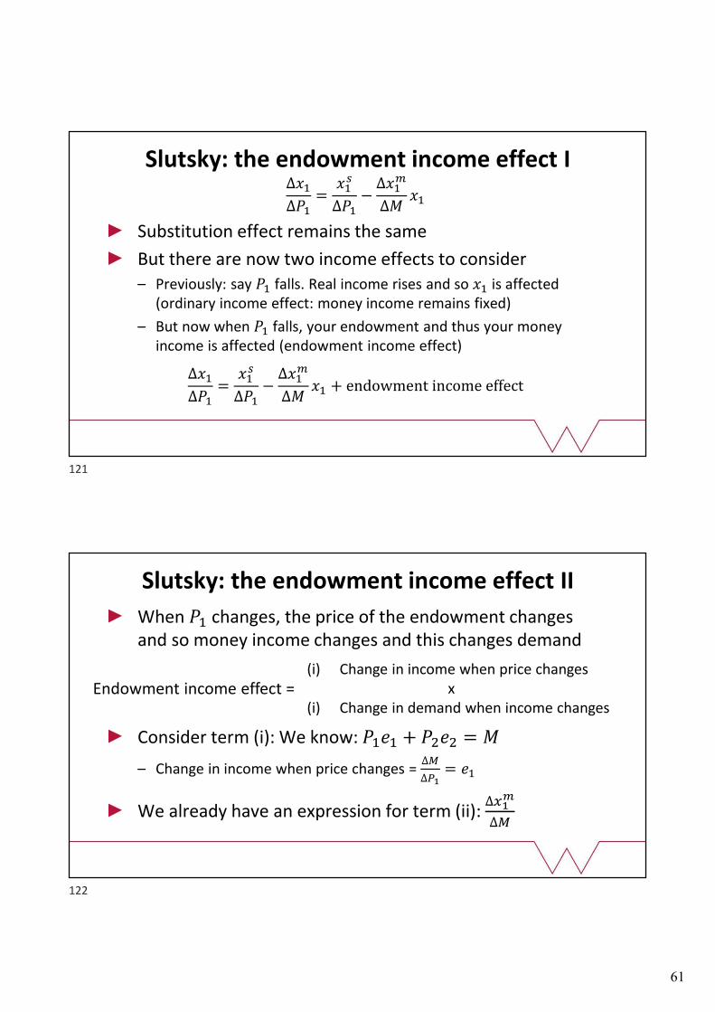
Slutsky: the endowment income effect I∆��

∆��=

���

∆��−

∆���

∆���

Substitution effect remains the same

But there are now two income effects to consider – Previously: say �� falls. Real income rises and so �� is affected

(ordinary income effect: money income remains fixed)

– But now when �� falls, your endowment and thus your money income is affected (endowment income effect)

∆��

∆��=

���

∆��−

∆���

∆��� + endowment income effect

Slutsky: the endowment income effect II

When �� changes, the price of the endowment changes and so money income changes and this changes demand

Consider term (i): We know: ���� + ���� = �

– Change in income when price changes = ∆�

∆��= ��

We already have an expression for term (ii): ∆��

�

∆�

Endowment income effect =(i) Change in income when price changes

x(i) Change in demand when income changes

121

122

62

Slutsky: the endowment income effect III

Endowment income effect:

Revised Slutsky equation:

Substitution effect is always negative: �� ↑ → ↓ ��

With a normal good: ordinary income effect > 0

Size of total effect depends on sign of (��−��): – Net demander: Price of normal good rises, demand must fall

– Net supplier: It depends on the magnitude of the positive combined income effect, versus negative substitution effect

∆���

∆�

∆�

∆��=

∆���

∆���

∆��

∆��=

���

∆��+ (�� − ��)

∆���

∆�

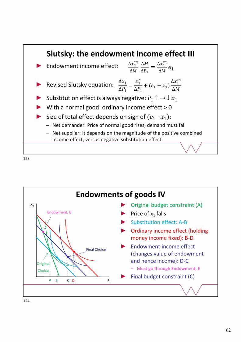
Endowments of goods IVOriginal budget constraint (A)

Price of x1 falls

Substitution effect: A-B

Ordinary income effect (holding money income fixed): B-D

Endowment income effect (changes value of endowment and hence income): D-C– Must go through Endowment, E

Final budget constraint (C)A

X2

X1

Endowment, E

Final Choice

C DB

Original

Choice

123

124

63

Should you go to university?– No: You’ll have a low income as a student and will incur huge debts

– Yes: You’ll have a higher income as a graduate and pensioner

We can apply the consumer choice model to consider:– How much debt should you accumulate as a student?

– How will the amount of debt depend on the interest rate?

– How much should you save for retirement?

This model is crucial to understanding saving decisions

We treat two time periods (t = 1, 2) exactly like two goods

Intertemporal Choice I

I can earn £10,000 (m1) this summer and then travel next summer, earning £0 (m2). Assume r = 10%– If c1 = 0, I could consume [�� 1 + 0.1 + ��] next summer.

– For every £1 consumed today, next year’s consumption falls by (1+r)

– The most I have for consumption next summer is what I would have had if c1 = 0 minus (1+r) times my actual consumption this summer

�� ≤ �� 1 + � + �� − 1 + � ��

1 + � �� + �� ≤ �� 1 + � + ��

�� + ��(1 + �)��≤ �� + ��(1 + �)��

Intertemporal Choice II

Future value

Present value

Rearranging gives:

125

126

64

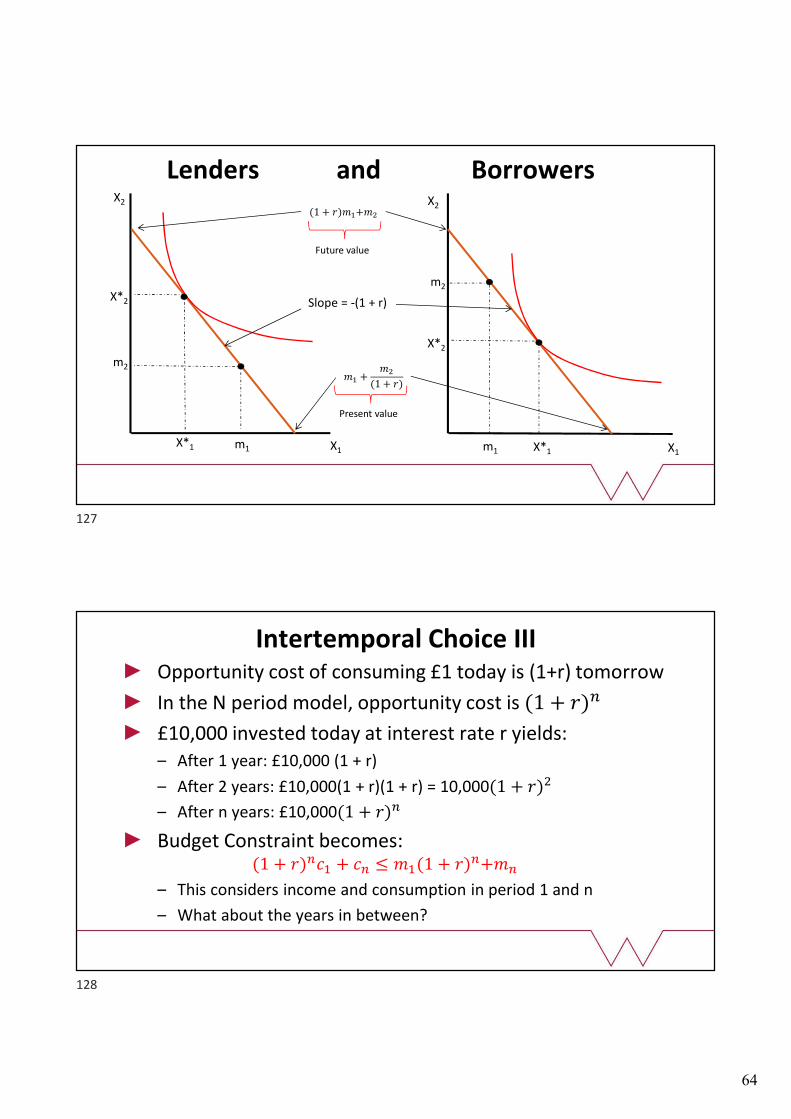
Lenders and Borrowers

m1

m2

X*1

X*2

X2

X1

Slope = -(1 + r)

�� +��

(1 + �)

Present value

(1 + �)��+��

Future value

m1

m2

X*1

X*2

X2

X1

Opportunity cost of consuming £1 today is (1+r) tomorrow

In the N period model, opportunity cost is (1 + �)�

£10,000 invested today at interest rate r yields:– After 1 year: £10,000 (1 + r)

– After 2 years: £10,000(1 + r)(1 + r) = 10,000(1 + �)�

– After n years: £10,000(1 + �)�

Budget Constraint becomes:(1 + �)��� + �� ≤ ��(1 + �)�+��

– This considers income and consumption in period 1 and n

– What about the years in between?

Intertemporal Choice III

127

128

65

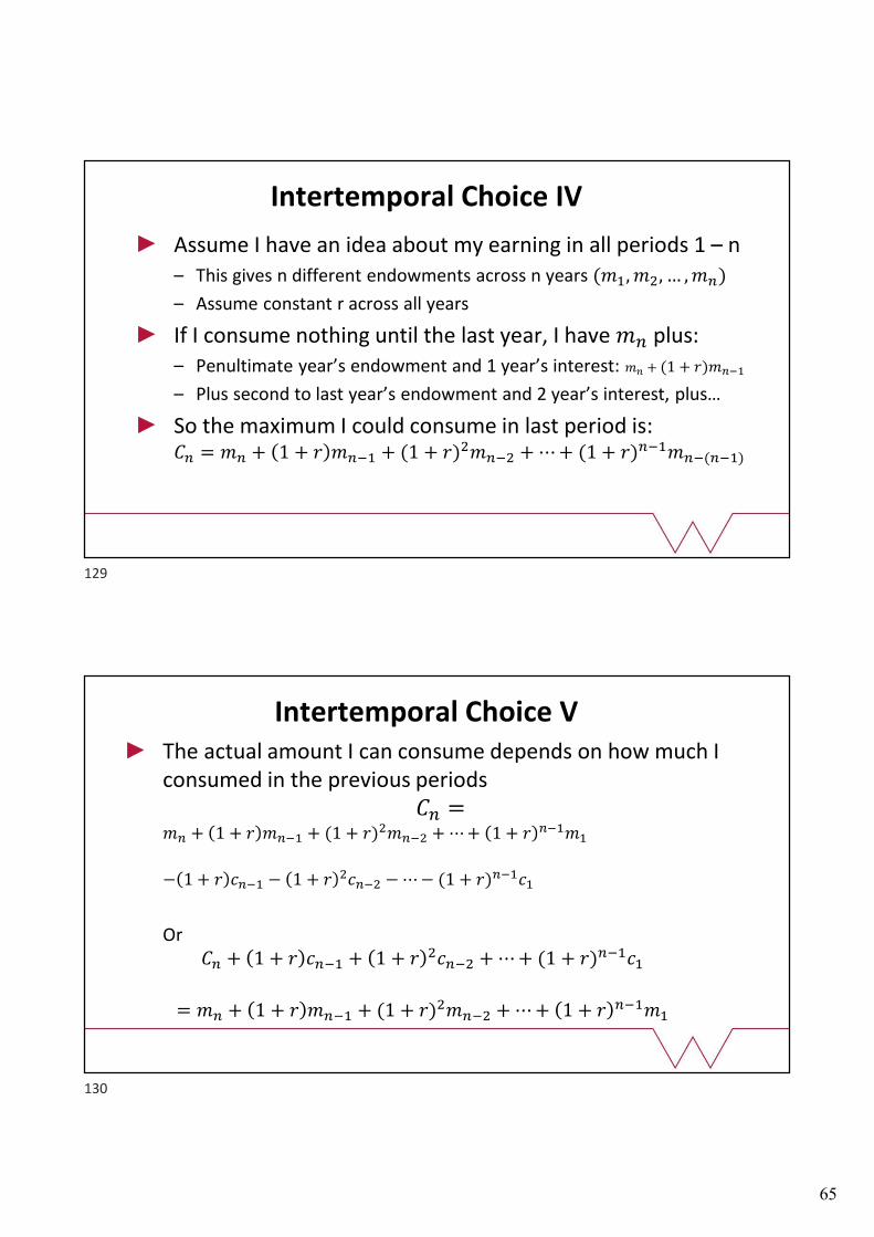
Assume I have an idea about my earning in all periods 1 – n– This gives n different endowments across n years (��, ��, … , ��)

– Assume constant r across all years

If I consume nothing until the last year, I have �� plus:– Penultimate year’s endowment and 1 year’s interest: �� + (1 + �)����

– Plus second to last year’s endowment and 2 year’s interest, plus…

So the maximum I could consume in last period is:�� = �� + 1 + � ���� + (1 + �)����� + ⋯ + (1 + �)������(���)

Intertemporal Choice IV

The actual amount I can consume depends on how much I consumed in the previous periods

�� =�� + 1 + � ���� + (1 + �)����� + ⋯ + 1 + � �����

− 1 + � ���� − 1 + � ����� − ⋯ − (1 + �)�����

Or�� + 1 + � ���� + 1 + � ����� + ⋯ + (1 + �)�����

= �� + 1 + � ���� + (1 + �)����� + ⋯ + 1 + � �����

Intertemporal Choice V

129

130

66

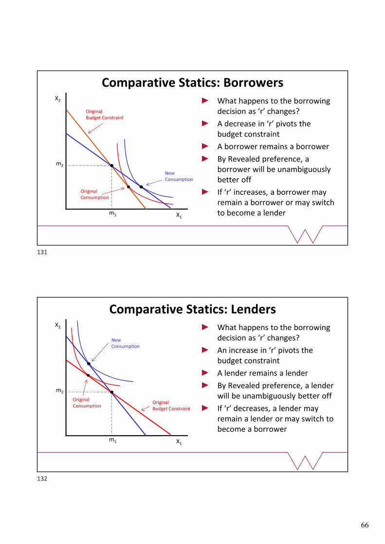
Comparative Statics: BorrowersWhat happens to the borrowing decision as ‘r’ changes?

A decrease in ‘r’ pivots the budget constraint

A borrower remains a borrower

By Revealed preference, a borrower will be unambiguously better off

If ‘r’ increases, a borrower may remain a borrower or may switch to become a lender

X2

X1m1

m2

OriginalConsumption

NewConsumption

OriginalBudget Constraint

Comparative Statics: LendersWhat happens to the borrowing decision as ‘r’ changes?

An increase in ‘r’ pivots the budget constraint

A lender remains a lender

By Revealed preference, a lender will be unambiguously better off

If ‘r’ decreases, a lender may remain a lender or may switch to become a borrower

X2

X1m1

m2

OriginalConsumption

NewConsumption

OriginalBudget Constraint

131

132

67

We can apply the consumer choice model to many areasand it can give important insights to policy-makers– Should taxes be increased on certain goods?

– If interest rates change, how will this affect the behaviour of savers and borrowers?

– If income tax rises, what happens to the supply of labour?

– If in-work or out-of-work benefits change, how will this affect people’s incentive to work?

You will look at a further application in seminars

Applications

133

31/10/2019

1

EC109

Production Theory

Elizabeth Jones

The Topics

Production functions

Isoquants and MRTS

Returns to scale

Cost functions and cost curves

Cost minimization

Expansion paths

Comparative statics

Short versus long run

Profit functions

Supply functions

31/10/2019

2

The firm’s problem

Firms make choices:

Which inputs should be used, e.g. capital and labour?

Firms face constraints:

Technological constraints, e.g. how easy it is to convert inputs into outputs?

Which combinations of inputs will produce a given level of output?

Economic constraints that derive from the prices of inputs and outputs

Maximise profit: difference between revenue and costs

Given input prices, what’s the cheapest way to produce a given quantity?

Given output prices, how much should the firm produce?

Production Functions

31/10/2019

3

Production functions

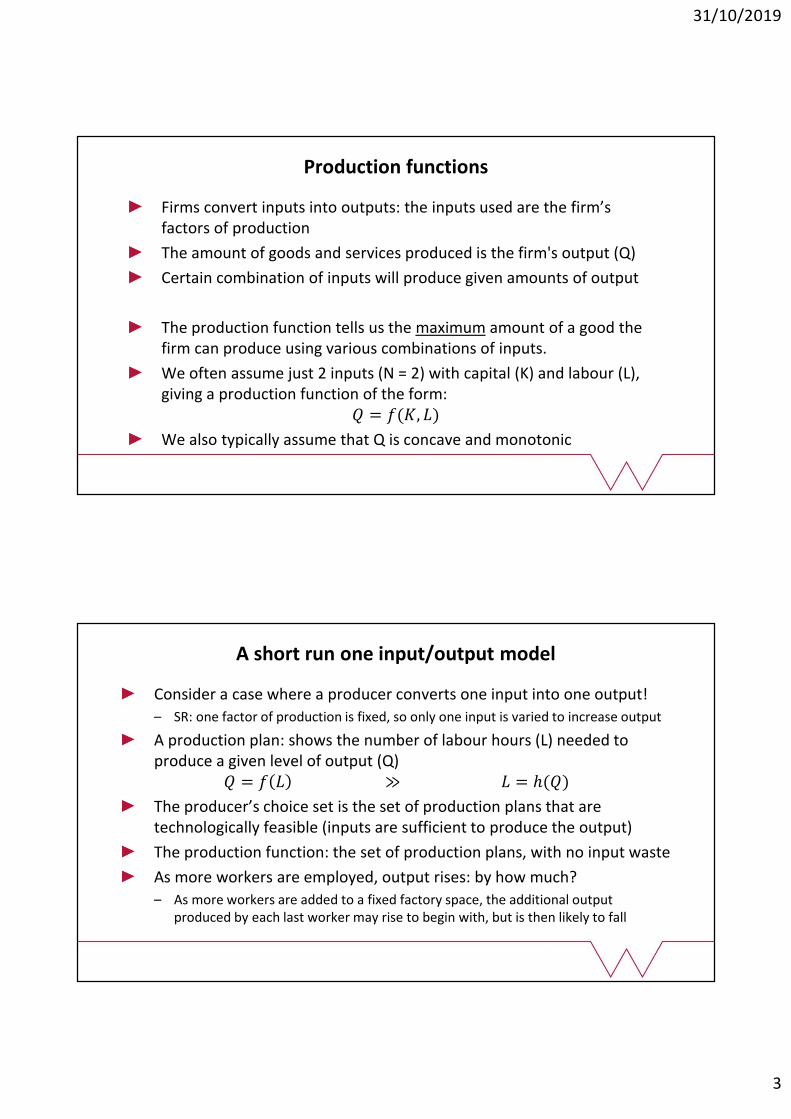
Firms convert inputs into outputs: the inputs used are the firm’s factors of production

The amount of goods and services produced is the firm's output (Q)

Certain combination of inputs will produce given amounts of output

The production function tells us the maximum amount of a good the firm can produce using various combinations of inputs.

We often assume just 2 inputs (N = 2) with capital (K) and labour (L), giving a production function of the form:

� = �(�, �)

We also typically assume that Q is concave and monotonic

A short run one input/output model

Consider a case where a producer converts one input into one output!

– SR: one factor of production is fixed, so only one input is varied to increase output

A production plan: shows the number of labour hours (L) needed to produce a given level of output (Q)

� = � � ≫ � = ℎ(�)

The producer’s choice set is the set of production plans that are technologically feasible (inputs are sufficient to produce the output)

The production function: the set of production plans, with no input waste

As more workers are employed, output rises: by how much?

– As more workers are added to a fixed factory space, the additional output produced by each last worker may rise to begin with, but is then likely to fall

31/10/2019

4

Production functions

• B uses 20 labour hours to produce 80 units

• What can we say about C and D?

Why does the slope on this production function initially get steeper and then get shallower?

Marginal and Average Product

Marginal product of Labour: The additional output produced by one more worker (or labour hour)

��� =�ℎ���� in total product

�ℎ���� in quantity of labour=

∆�

∆�=

��

��= ��

Linear Production function: Constant ���

We normally assume diminishing marginal productivity (flatter function)

����

��=

���

���< 0

Average product of Labour:

��� =Total product

Quantity of labour=

�

�=

�(�, �)

�

31/10/2019

5

0

10

20

30

40

0 1 2 3 4 5 6 7 8

-2

0

2

4

6

8

10

12

14

0 1 2 3 4 5 6 7 8

Tonnes o

f w

heat

per

year

Tonnes o

f w

heat

per

year

Number of farm workers (L)

Marginal and Average ProductFrom the total product function, we can derive the marginal and average product of labour curves.

Point D: Law of diminishing marginal returns:

As variable input increases, with others held fixed, a point will be reached beyond which the marginal product of the variable input will decrease.

Point E: maximum output (MPL= 0)

��� at 5� is the slope of AB

��� at 2� is the slope of OC

Two inputs - Robots and humans

Assume now that production requires both Capital and Labour.

0

6

12

18

2430

0

50

100

150

200

06

1218

2430

Thousands of machine hours/ day

Thousands of man hours/ day

Q, thousands of economist cards/day

�

0 6 12 18 24 30

0 0 0 0 0 0 0

6 0 5 15 25 30 23

L 12 0 15 48 81 96 75

18 0 25 81 137 162 127

24 0 30 96 162 192 150

30 0 23 75 127 150 117

��� =�ℎ���� in total product

�ℎ���� in quantity of ������=

∆�

∆�=

��

��= ��

We can now find marginal products of capital and labour

��� =�ℎ���� in total product

�ℎ���� in quantity of �������=

∆�

∆�=

��

��= ��

31/10/2019

6

Isoquants

Isoquants

Isoquants show all combinations of labour and capital that produce a given level of output (Q0)

� �, � = ��

K, 0

00s

of

mac

hin

e h

ou

r a

day

L, 000s of Labour hours a day

�

0 6 12 18 24 30

0 0 0 0 0 0 0

6 0 5 15 25 30 23

L 12 0 15 48 81 96 75

18 0 25 81 137 162 127

24 0 30 96 162 192 150

30 0 23 75 127 150 117

18

6

6

18

31/10/2019

7

Marginal rate of Technical Substitution

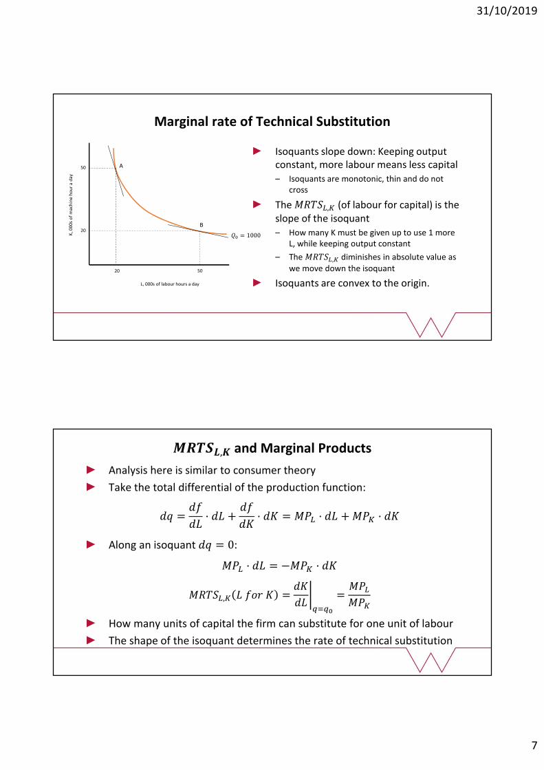
Isoquants slope down: Keeping output constant, more labour means less capital– Isoquants are monotonic, thin and do not

cross

The �����,� (of labour for capital) is the slope of the isoquant– How many K must be given up to use 1 more

L, while keeping output constant

– The �����,� diminishes in absolute value as

we move down the isoquant

Isoquants are convex to the origin.

K, 0

00s

of

mac

hin

e h

ou

r a

day

L, 000s of labour hours a day

20 50

20

50

�� = 1000

A

B

�����,� and Marginal Products

Analysis here is similar to consumer theory

Take the total differential of the production function:

�� =��

��· �� +

��

��· �� = ��� · �� + ��� · ��

Along an isoquant �� = 0:

��� · �� = −��� · ��

�����,� � ��� � =��

���

����

=���

���

How many units of capital the firm can substitute for one unit of labour

The shape of the isoquant determines the rate of technical substitution

31/10/2019

8

Isoquants versus indifference curves

Indifference curves represents tastes, while isoquants arise from production functions, which are the technological constraints faced by producers

Utility is not measureable, meaning there is no objective interpretation as to the numbers accompanying indifference curves, beyond the ordering.

Isoquants reflect output which is measurable

– Doubling all values associated with an indifference map leaves us with the same tastes as before

– Doubling all values associated with isoquants alters the production technology, with the new technology producing twice as much output from any bundle of inputs (Returns to scale)

Convexity under Producer Theory

Vertical and horizontal slices

are convex: concave production function

Only horizontal slices

are convex: quasi-concave production function

31/10/2019

9

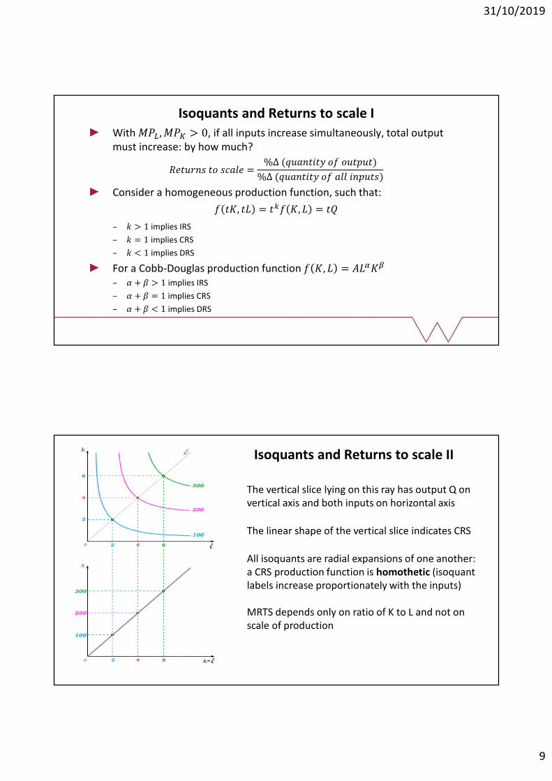
Isoquants and Returns to scale I

With ���, ��� > 0, if all inputs increase simultaneously, total output must increase: by how much?

������� �� ����� =%∆ (�������� �� ������)

%∆ (�������� �� ��� ������)

Consider a homogeneous production function, such that:

� ��, �� = ��� �, � = ��

– � > 1 implies IRS

– � = 1 implies CRS

– � < 1 implies DRS

For a Cobb-Douglas production function � �, � = �����

– � + � > 1 implies IRS

– � + � = 1 implies CRS

– � + � < 1 implies DRS

Isoquants and Returns to scale II

The vertical slice lying on this ray has output Q on vertical axis and both inputs on horizontal axis

The linear shape of the vertical slice indicates CRS

All isoquants are radial expansions of one another: a CRS production function is homothetic (isoquant labels increase proportionately with the inputs)

MRTS depends only on ratio of K to L and not on scale of production

31/10/2019

10

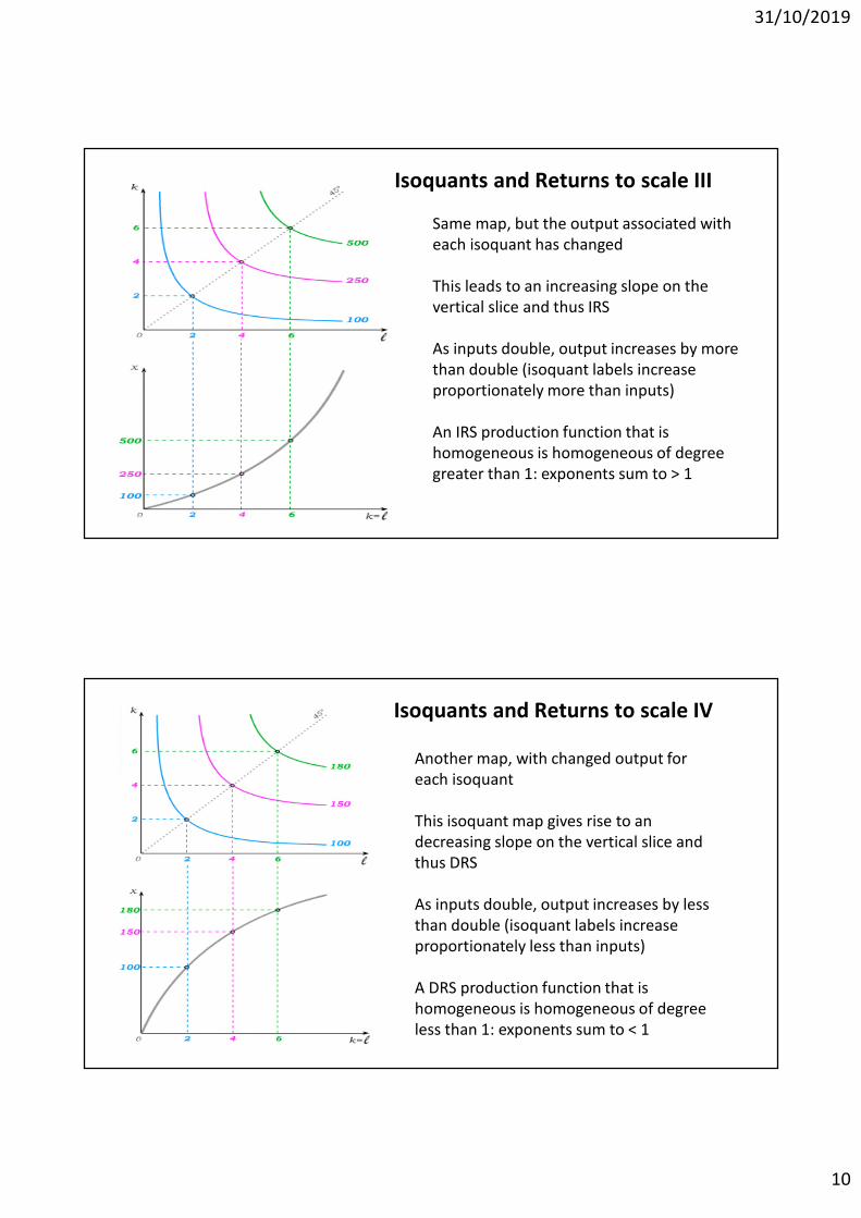
Isoquants and Returns to scale III

Same map, but the output associated with each isoquant has changed

This leads to an increasing slope on the vertical slice and thus IRS

As inputs double, output increases by more than double (isoquant labels increase proportionately more than inputs)

An IRS production function that is homogeneous is homogeneous of degree greater than 1: exponents sum to > 1

Another map, with changed output for each isoquant

This isoquant map gives rise to an decreasing slope on the vertical slice and thus DRS

As inputs double, output increases by less than double (isoquant labels increase proportionately less than inputs)

A DRS production function that is homogeneous is homogeneous of degree less than 1: exponents sum to < 1

Isoquants and Returns to scale IV

31/10/2019

11

K, u

nit

s o

f ca

pit

al p

er

year

L, units of labour per year

� = 100� = 140

� = 170� = 200

� = 300

A

D

E

BC

10 20 30

30

20

10

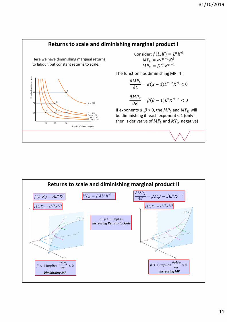
Returns to scale and diminishing marginal product I

Here we have diminishing marginal returns to labour, but constant returns to scale.

Consider: � �, � = ����

��� = �������

��� = �������

The function has diminishing MP iff:

����

��= � � − 1 ������ < 0

����

��= � � − 1 ������ < 0

If exponents �, � > 0, the ��� and ��� will be diminishing iff each exponent < 1 (only then is derivative of ��� and ��� negative)

Marginal Product and Returns to Scale

+b > 1 impliesIncreasing Returns to Scale

Diminishing MP Increasing MP

� �, � = ����� ��� = �������� ����

��= �� � − 1 ������

�(�, �) = ��/���/� �(�, �) = ��/���/�

� < 1 ������� ����

��< 0 � > 1 �������

����

��> 0

Returns to scale and diminishing marginal product II

31/10/2019

12

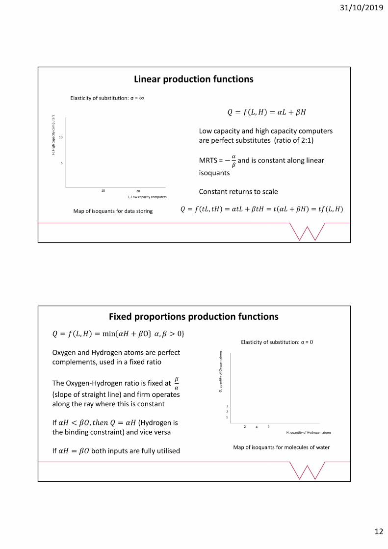
Linear production functions

H, H

igh

cap

acit

y co

mp

ute

rs

L, Low capacity computers

10 20

5

10

Map of isoquants for data storing

� = � �, � = �� + ��

Low capacity and high capacity computers are perfect substitutes (ratio of 2:1)

MRTS = −�

�and is constant along linear

isoquants

Constant returns to scale

Elasticity of substitution: σ = ∞

� = � ��, �� = ��� + ��� = � �� + �� = ��(�, �)

Fixed proportions production functions

O,q

uan

tity

of

Oxy

gen

ato

ms

H, quantity of Hydrogen atoms

2

1

3

4 6

2

Map of isoquants for molecules of water

� = � �, � = min �� + �O �, � > 0}

Oxygen and Hydrogen atoms are perfect complements, used in a fixed ratio

The Oxygen-Hydrogen ratio is fixed at �

�

(slope of straight line) and firm operates along the ray where this is constant

If �� < ��, �ℎ�� � = �� (Hydrogen is the binding constraint) and vice versa

If �� = �� both inputs are fully utilised

Elasticity of substitution: σ = 0

31/10/2019

13

Cobb Douglas production function

K, u

nit

s o

f ca

pit

al p

er

day

L, units of labour per day

10

30

40

20

10

20 30 40 50

50

� = ����� �, �, � > 0

Inputs substitutable in variable proportions along an isoquant

It can exhibit any returns to scale, depending on if (� + �) >, <, = 1

���� =���

���

The CD function is linear in logarithms:

��� = ��� + ���� + ����

� is elasticity of output with respect to L� is elasticity of output with respect to K

Elasticity of substitution: σ = 1

Costs

31/10/2019

14

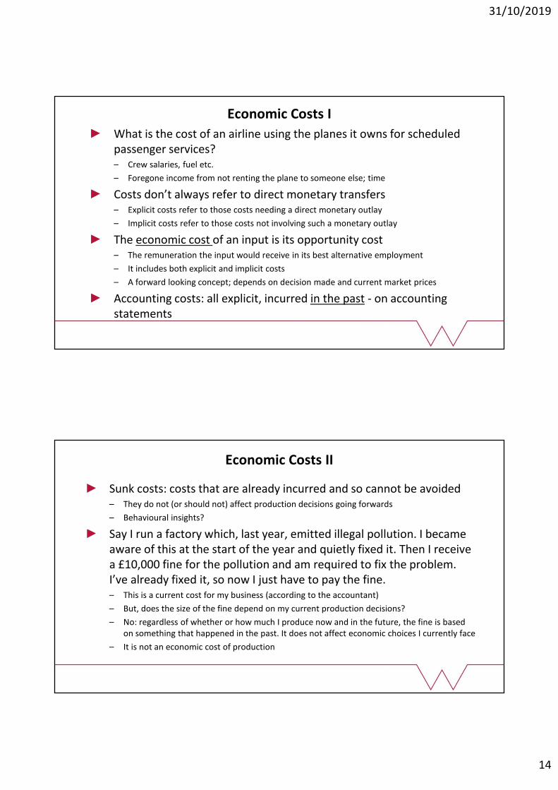
Economic Costs I

What is the cost of an airline using the planes it owns for scheduled passenger services?– Crew salaries, fuel etc.

– Foregone income from not renting the plane to someone else; time

Costs don’t always refer to direct monetary transfers– Explicit costs refer to those costs needing a direct monetary outlay

– Implicit costs refer to those costs not involving such a monetary outlay

The economic cost of an input is its opportunity cost– The remuneration the input would receive in its best alternative employment

– It includes both explicit and implicit costs

– A forward looking concept; depends on decision made and current market prices

Accounting costs: all explicit, incurred in the past - on accounting statements

Economic Costs II

Sunk costs: costs that are already incurred and so cannot be avoided– They do not (or should not) affect production decisions going forwards

– Behavioural insights?

Say I run a factory which, last year, emitted illegal pollution. I became aware of this at the start of the year and quietly fixed it. Then I receive a £10,000 fine for the pollution and am required to fix the problem. I’ve already fixed it, so now I just have to pay the fine.– This is a current cost for my business (according to the accountant)

– But, does the size of the fine depend on my current production decisions?

– No: regardless of whether or how much I produce now and in the future, the fine is based on something that happened in the past. It does not affect economic choices I currently face

– It is not an economic cost of production

31/10/2019

15

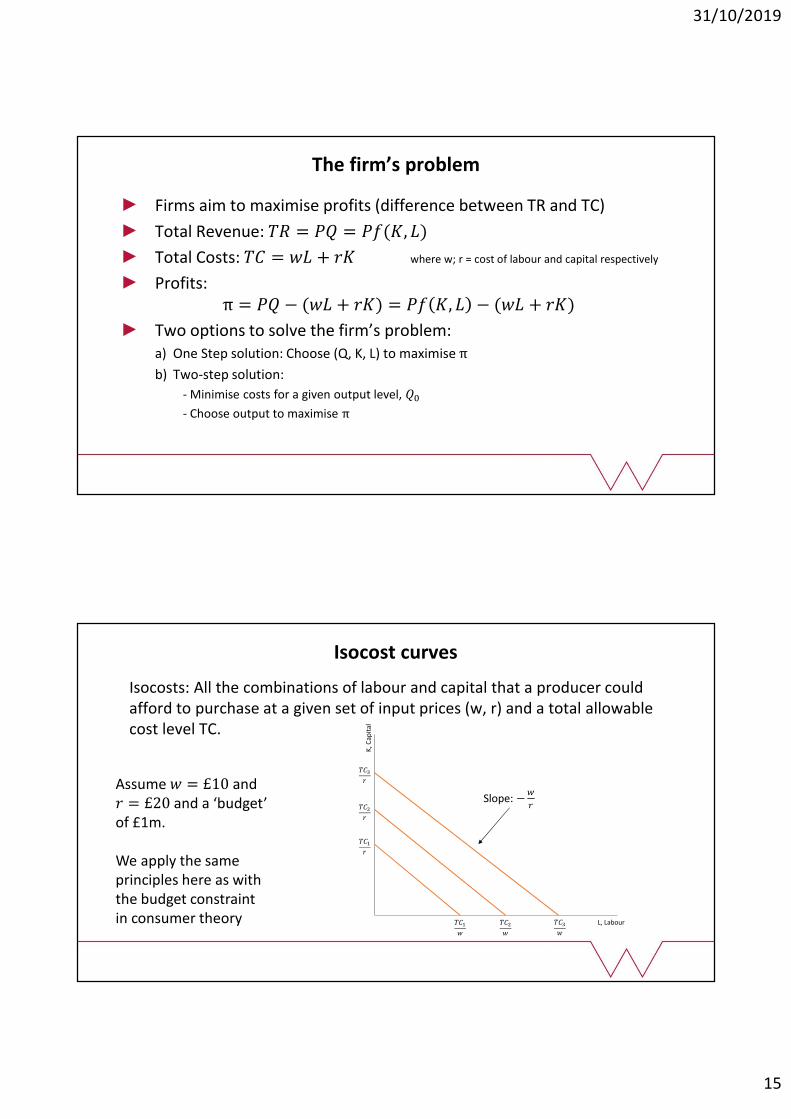
The firm’s problem

Firms aim to maximise profits (difference between TR and TC)

Total Revenue: �� = �� = ��(�, �)

Total Costs: �� = �� + �� where w; r = cost of labour and capital respectively

Profits: π = �� − (�� + ��) = �� �, � − (�� + ��)

Two options to solve the firm’s problem:a) One Step solution: Choose (Q, K, L) to maximise π

b) Two-step solution:

- Minimise costs for a given output level, ��

- Choose output to maximise π

Isocost curves

Isocosts: All the combinations of labour and capital that a producer could afford to purchase at a given set of input prices (w, r) and a total allowable cost level TC.

K, C

apit

al

L, Labour

���

�

���

�

���

�

���

�

���

�

���

�

Assume � = £10 and � = £20 and a ‘budget’ of £1m.

We apply the same principles here as with the budget constraint in consumer theory

Slope: −�

�

31/10/2019

16

K, C

apit

al

L, Labour

���

�

���

�

���

�

���

�

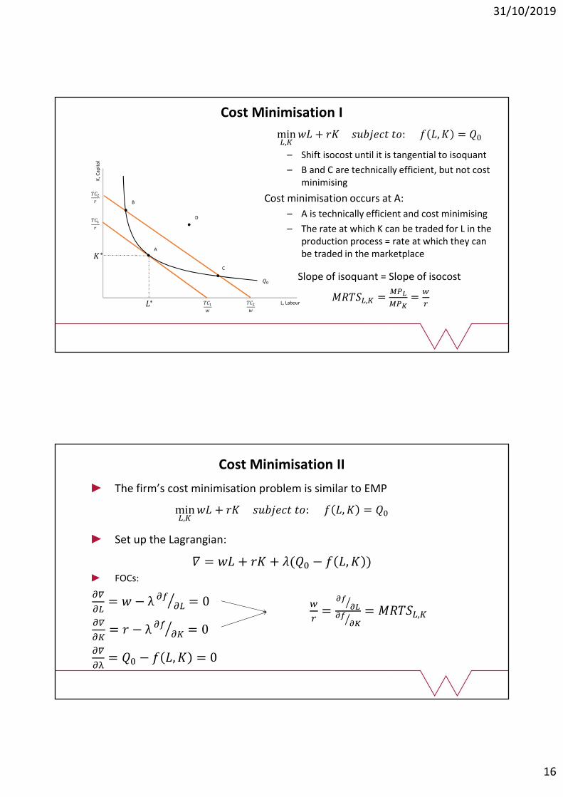
Cost Minimisation I

�∗

�∗

min�,�

�� + �� ������� ��: � �, � = ��

– Shift isocost until it is tangential to isoquant

– B and C are technically efficient, but not cost minimising

Cost minimisation occurs at A:

– A is technically efficient and cost minimising

– The rate at which K can be traded for L in the production process = rate at which they can be traded in the marketplace

Slope of isoquant = Slope of isocost

�����,� =���

���=

�

�

D

C

A

B

��

The firm’s cost minimisation problem is similar to EMP

min�,�

�� + �� ������� ��: � �, � = ��

Set up the Lagrangian:

� = �� + �� + �(�� − � �, � )FOCs:

��

��= � − λ ��

��� = 0

��

��= � − λ ��

��� = 0

��

��= �� − � �, � = 0

Cost Minimisation II

�

�=

����

�

�����

= �����,�

31/10/2019

17

�

�=

����

�

�����

=���

���= �����,�

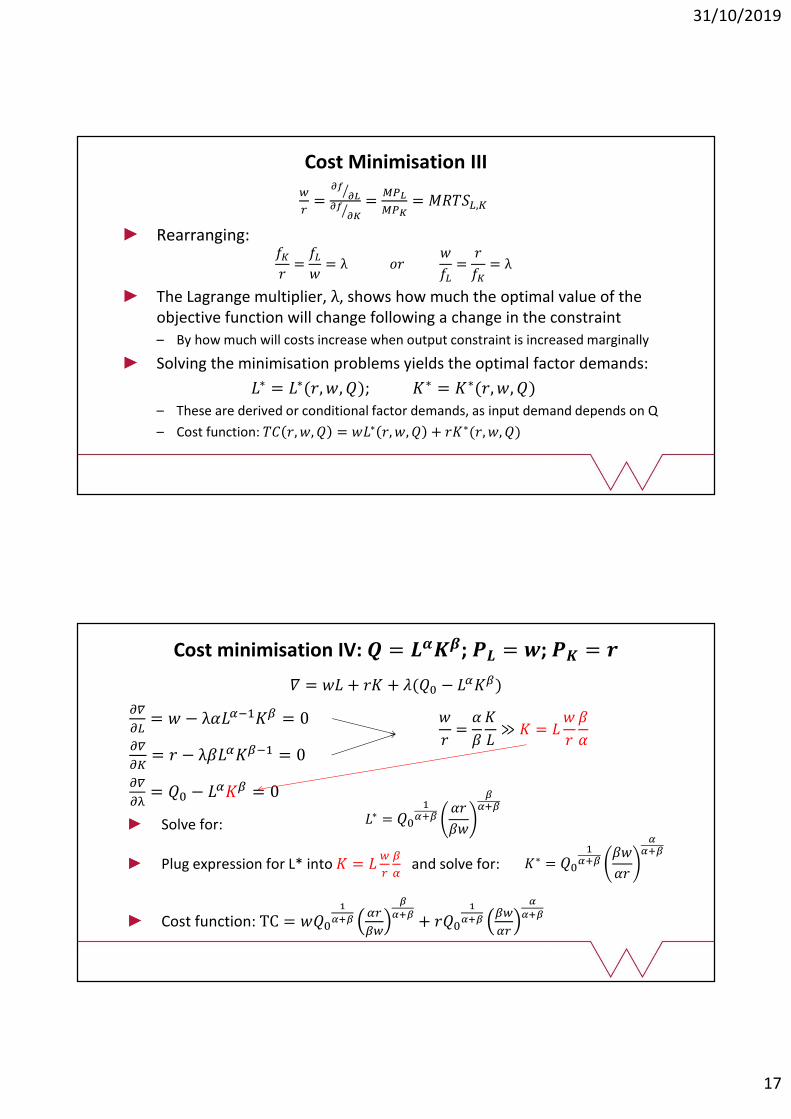
Rearranging:��

�=

��

�= λ ��

�

��=

�

��= λ

The Lagrange multiplier, λ, shows how much the optimal value of the objective function will change following a change in the constraint

– By how much will costs increase when output constraint is increased marginally

Solving the minimisation problems yields the optimal factor demands:

�∗ = �∗(�, �, �); �∗ = �∗(�, �, �)

– These are derived or conditional factor demands, as input demand depends on Q

– Cost function: �� �, �, � = ��∗ �, �, � + ��∗(�, �, �)

Cost Minimisation III

Cost minimisation IV: � = ����; �� = �; �� = �

� = �� + �� + �(�� − ����)

��

��= � − λ������� = 0

��

��= � − λ������� = 0

��

��= �� − ���� = 0

Solve for:

Plug expression for L* into � = ��

�

�

�and solve for:

Cost function: TC = ���

�

�����

��

�

���+ ���

�

�����

��

�

���

�

�=

�

�

�

�≫ � = �

�

�

�

�

�∗ = ��

����

��

��

����

�∗ = ��

����

��

��

����

31/10/2019

18

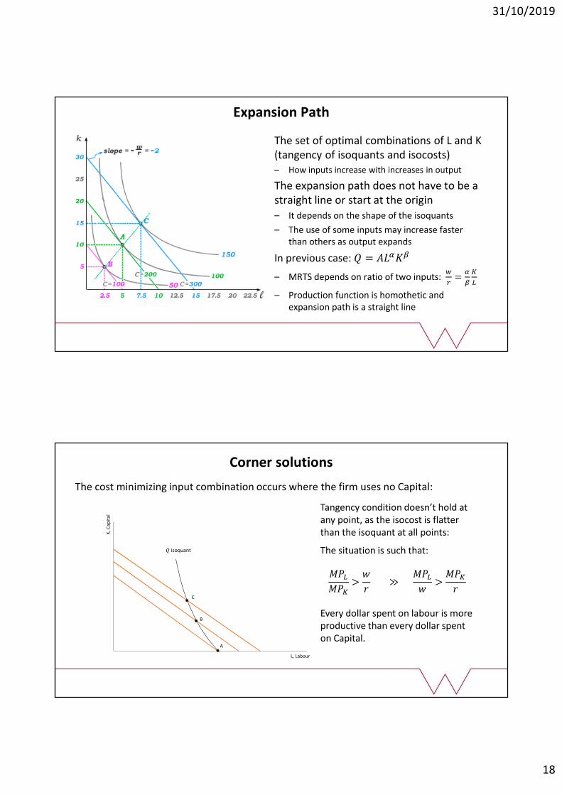
Expansion Path

The set of optimal combinations of L and K (tangency of isoquants and isocosts)– How inputs increase with increases in output

The expansion path does not have to be a straight line or start at the origin– It depends on the shape of the isoquants

– The use of some inputs may increase faster than others as output expands

In previous case: � = �����

– MRTS depends on ratio of two inputs: �

�=

�

�

�

�

– Production function is homothetic and expansion path is a straight line

Corner solutions

The cost minimizing input combination occurs where the firm uses no Capital:

K, C

apit

al

L, Labour

B

A

C

� isoquant

Tangency condition doesn’t hold at any point, as the isocost is flatter than the isoquant at all points:

The situation is such that:

���

���>

�

� ≫

���

�>

���

�

Every dollar spent on labour is more productive than every dollar spent on Capital.

31/10/2019

19

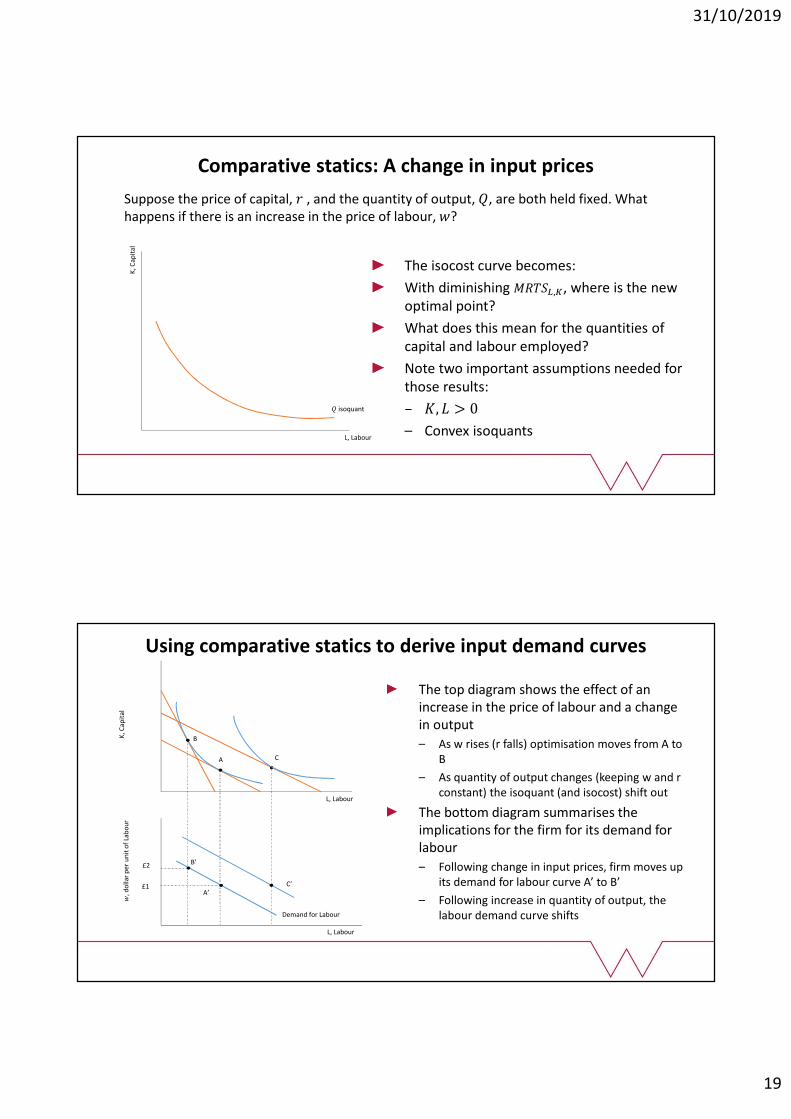
Comparative statics: A change in input prices

Suppose the price of capital, � , and the quantity of output, �, are both held fixed. What happens if there is an increase in the price of labour, �?

K, C

apit

al

L, Labour

� isoquant

The isocost curve becomes:

With diminishing �����,�, where is the new optimal point?

What does this mean for the quantities of capital and labour employed?

Note two important assumptions needed for those results:

– �, � > 0

– Convex isoquants

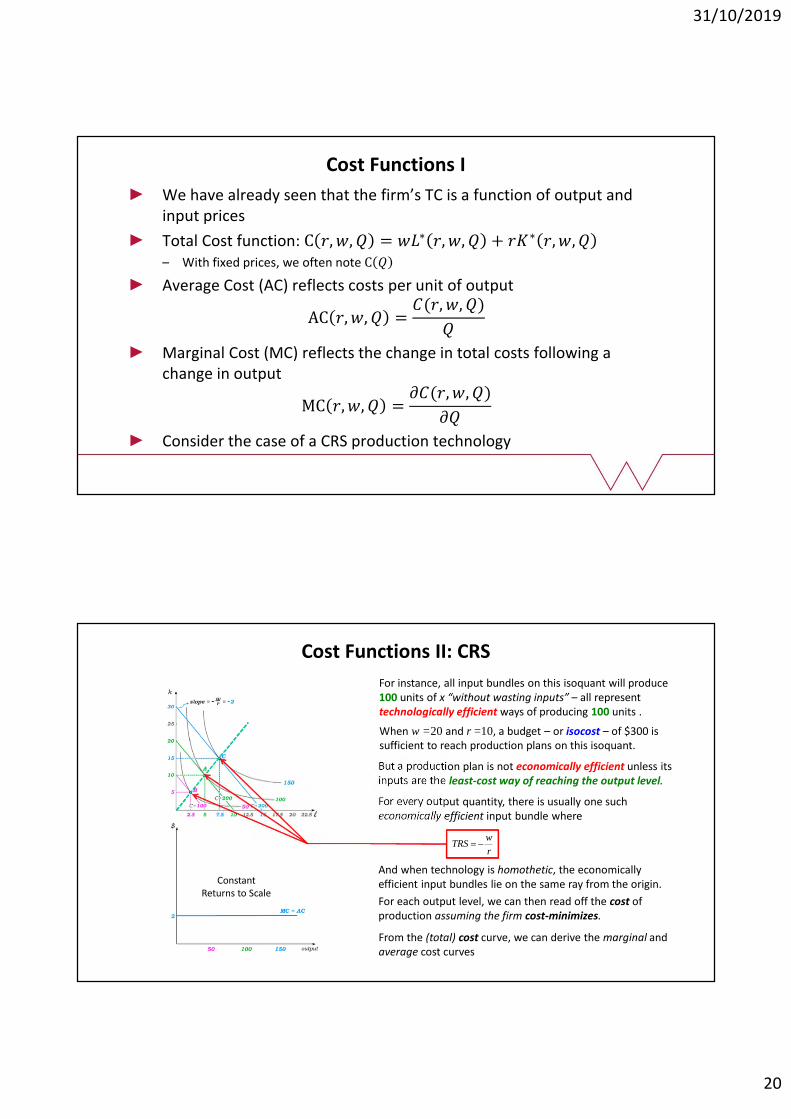
Using comparative statics to derive input demand curves

A

A’

C

B

B’

C’

L, Labour

K, C

apit

al

L, Labour

�, d

olla

r p

er u

nit

of

Lab

ou

r

£1

£2

Demand for Labour

The top diagram shows the effect of an increase in the price of labour and a change in output

– As w rises (r falls) optimisation moves from A to B

– As quantity of output changes (keeping w and r constant) the isoquant (and isocost) shift out

The bottom diagram summarises the implications for the firm for its demand for labour

– Following change in input prices, firm moves up its demand for labour curve A’ to B’

– Following increase in quantity of output, the labour demand curve shifts

31/10/2019

20

Cost Functions I

We have already seen that the firm’s TC is a function of output and input prices

Total Cost function: C �, �, � = ��∗ �, �, � + ��∗ �, �, �– With fixed prices, we often note C �

Average Cost (AC) reflects costs per unit of output

AC �, �, � =�(�, �, �)

�

Marginal Cost (MC) reflects the change in total costs following a change in output

MC �, �, � =��(�, �, �)

��

Consider the case of a CRS production technology

For instance, all input bundles on this isoquant will produce 100 units of x “without wasting inputs” – all represent technologically efficient ways of producing 100 units .

When w =20 and r =10, a budget – or isocost – of $300 is sufficient to reach production plans on this isoquant.

But a production plan is not economically efficient unless its inputs are the least-cost way of reaching the output level.

For every output quantity, there is usually one such economically efficient input bundle where

And when technology is homothetic, the economically efficient input bundles lie on the same ray from the origin.

For each output level, we can then read off the cost of production assuming the firm cost-minimizes.

From the (total) cost curve, we can derive the marginal and average cost curves

TRS w

r

Constant Returns to Scale

Cost Functions II: CRS

31/10/2019

21

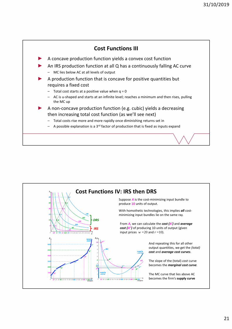
Cost Functions III

A concave production function yields a convex cost function

An IRS production function at all Q has a continuously falling AC curve– MC lies below AC at all levels of output

A production function that is concave for positive quantities but requires a fixed cost– Total cost starts at a positive value when q = 0

– AC is u-shaped and starts at an infinite level; reaches a minimum and then rises, pulling the MC up

A non-concave production function (e.g. cubic) yields a decreasing then increasing total cost function (as we’ll see next)– Total costs rise more and more rapidly once diminishing returns set in

– A possible explanation is a 3rd factor of production that is fixed as inputs expand

Suppose A is the cost-minimizing input bundle to produce 10 units of output.

With homothetic technologies, this implies all cost-minimizing input bundles lie on the same ray.

IRS

DRSFrom A, we can calculate the cost (A’) and average cost (A”) of producing 10 units of output (given input prices w =20 and r =10).

And repeating this for all other output quantities, we get the (total) cost and average cost curves.

The slope of the (total) cost curve becomes the marginal cost curve.

Cost Functions IV: IRS then DRS

The MC curve that lies above AC becomes the firm’s supply curve

31/10/2019

22

Properties of cost functions

Cost functions are homogenous of degree 1 in input prices– Doubling all input prices won’t change level of inputs used; inflation shifts cost curves up

Cost functions are non-decreasing in Q and in input prices

If Q = f(�, �) is convex, it exhibits IRS and C(w, r, �) is concave in Q:– MC(Q) and AC(Q) fall as Q rises: The firm benefits from economies of scale

If Q = f(�, �) is concave, it exhibits DRS and C(w, r, �) is convex in Q:– MC(Q) and AC(Q) rise as Q rises: The firm suffers from diseconomies of scale

With CRS, output increases proportionally to an increase in all inputs: AC(Q) remains constant: no economies or diseconomies of scale– When costs are minimised, the firm is productively efficient: minimum efficient scale

AC(Q) is increasing when MC(Q) ≥ AC(Q) and decreasing when MC(Q) ≤ AC(Q)

Shifting cost curves I

Any change in technology or input prices will shift the isocost curve and hence the cost function

Starting from point A, where the firm produces 1 million televisions, on isocost line ��.

After the price of capital increases, the cost minimising input combination to produce 1 million units occurs at point B

But, total cost is now greater than it was at point A

�� = �� < ��

1 million TV per year

A

B

Labour services per year

K, C

apit

al s

ervi

ces

��

��

��

31/10/2019

23

Shifting cost curves II

1000

��(�) after the

decrease in the

price of coal

Units of Output

B

A

��(�) before

the decrease in

the price of

coal

��

��

TC

, dol

lars

per

year

Coal fields in Pennsylvania and West Virginia were opened in 19th century, cutting the price of coal– Iron producers substituted coal for wood

– Fuel and cost curves for iron output shifted downwards

Cyberspace: acquiring information is now relatively cheaper with ‘IT’

This tilts LRTC down and cuts the cost for producing a given level of output (A to B)– Or level of output increases for the same costs

This may partly explain the breaking up of big companies from mid-1970s as the cost of information for smaller firms fell

Shifting cost curves III

Slope of CD =Marginal Cost

Slope of 0A = Average Cost

An increase in costs– Tilts TC(Q) upwards

– AC shifts upwards

– MC shifts upwards

The relationship between MC and AC is such that:• When AC is decreasing in Q,

�� � > ��(�)

• When AC is increasing in Q, �� � < ��(�)

• When AC is at a minimum, �� � = ��(�)

50 Q, units per year

A

TC

, dol

lars

£1,500

C

0

D

��(�)

A’

A’’

�� � = slope

of ��(�)�� � slope of ray from O

to ��(�)

£30

£10

50 Q, units per year

��

,��

, per

unit

B

B’

B’

31/10/2019

24

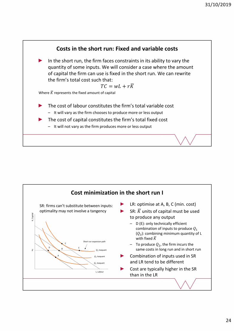
Costs in the short run: Fixed and variable costs

In the short run, the firm faces constraints in its ability to vary the quantity of some inputs. We will consider a case where the amount of capital the firm can use is fixed in the short run. We can rewrite the firm’s total cost such that:

�� = �� + ���

Where �� represents the fixed amount of capital

The cost of labour constitutes the firm’s total variable cost– It will vary as the firm chooses to produce more or less output

The cost of capital constitutes the firm’s total fixed cost– It will not vary as the firm produces more or less output

Cost minimization in the short run I

LR: optimise at A, B, C (min. cost)

SR: �� units of capital must be used to produce any output

– D (E): only technically efficient combination of inputs to produce ��

(��): combining minimum quantity of L with fixed ��

– To produce ��, the firm incurs the same costs in long run and in short run

Combination of inputs used in SR and LR tend to be different

Cost are typically higher in the SR than in the LR

K, C

apit

al

L, Labour

A

B

C

��

�� Isoquant

�� Isoquant

�� Isoquant

Short run expansion path

D E

SR: firms can’t substitute between inputs: optimality may not involve a tangency

31/10/2019

25

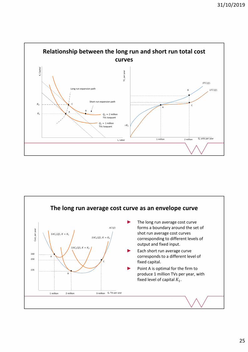
Relationship between the long run and short run total cost curves

K, C

apit

al

L, Labor

AB

C

��

�� = 1 million

TVs Isoquant

�� = 2 million

TVs isoquant

Short run expansion path��

Long run expansion path���(�)

Q, units per year

���(�)

���TC

, per

ye

ar

1 million

A

B

C

2 million

The long run average cost curve as an envelope curve

The long run average cost curve forms a boundary around the set of shot run average cost curves corresponding to different levels of output and fixed input.

Each short run average curve corresponds to a different level of fixed capital.

Point A is optimal for the firm to produce 1 million TVs per year, with fixed level of capital ��.

���� � , � = ��

���� � , � = ��

���� � , � = ��

�� �

A

B

C

1 million 2 million 3 million

£35

£50

£60

Co

st, p

er

year

Q, TVs per year

31/10/2019

26

Profit Maximisation

Profit Maximisation: 2 step problem

– Minimise costs for a given output level (already done)

– Choose output to maximise π (i.e. revenue minus costs)

Step 2 involves: ����� = �� − �(�, �, �)

This is an unconstrained maximisation problem

���: ��

��= � −

�� �, �, �

��= 0 ≫ � =

�� �, �, �

��= ��(�)

If revenue from last unit exceeds cost from last unit, then produce more

As ���(�)

��≥ 0 MC must slope upwards at the optimum

Solving yields optimal output: �∗ �, �, �

And Profit: �(�, �, �) = ��∗ − �(�, �, �∗)

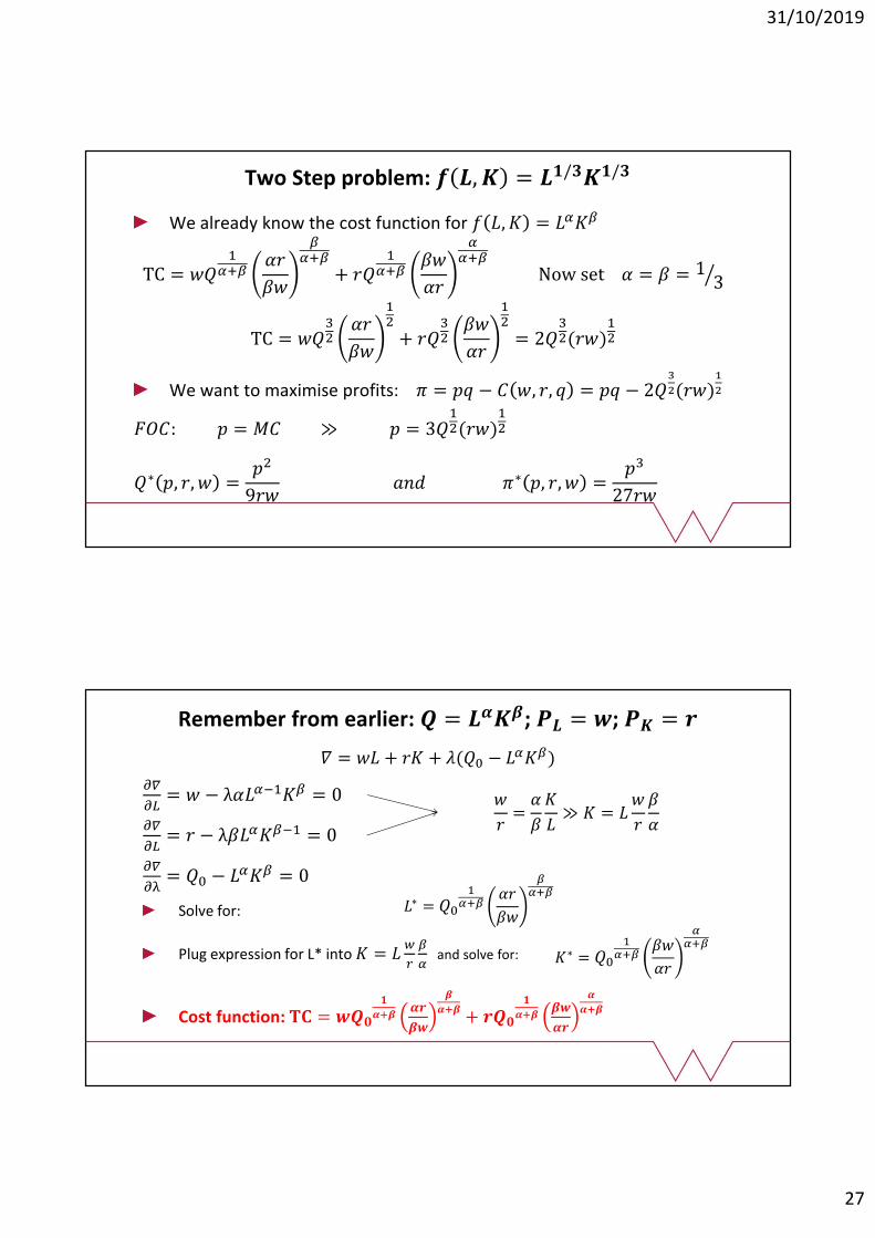
31/10/2019

27

Two Step problem: � �, � = ��/���/�

We already know the cost function for � �, � = ����

TC = ���

�����

��

����

+ ���

�����

��

����

Now set � = � = 13�

TC = ����

��

��

��

+ ����

��

��

��

= 2���(��)

��

We want to maximise profits: � = �� − � �, �, � = �� − 2��

�(��)�

�

���: � = �� ≫ � = 3���(��)

��

�∗ �, �, � =��

9�� ��� �∗ �, �, � =

��

27��

Remember from earlier: � = ����; �� = �; �� = �

� = �� + �� + �(�� − ����)

��

��= � − λ������� = 0

��

��= � − λ������� = 0

��

��= �� − ���� = 0

Solve for:

Plug expression for L* into � = ��

�

�

�and solve for:

Cost function: �� = ���

�

�����

��

�

���+ ���

�

�����

��

�

���

�

�=

�

�

�

�≫ � = �

�

�

�

�

�∗ = ��

����

��

��

����

�∗ = ��

����

��

��

����

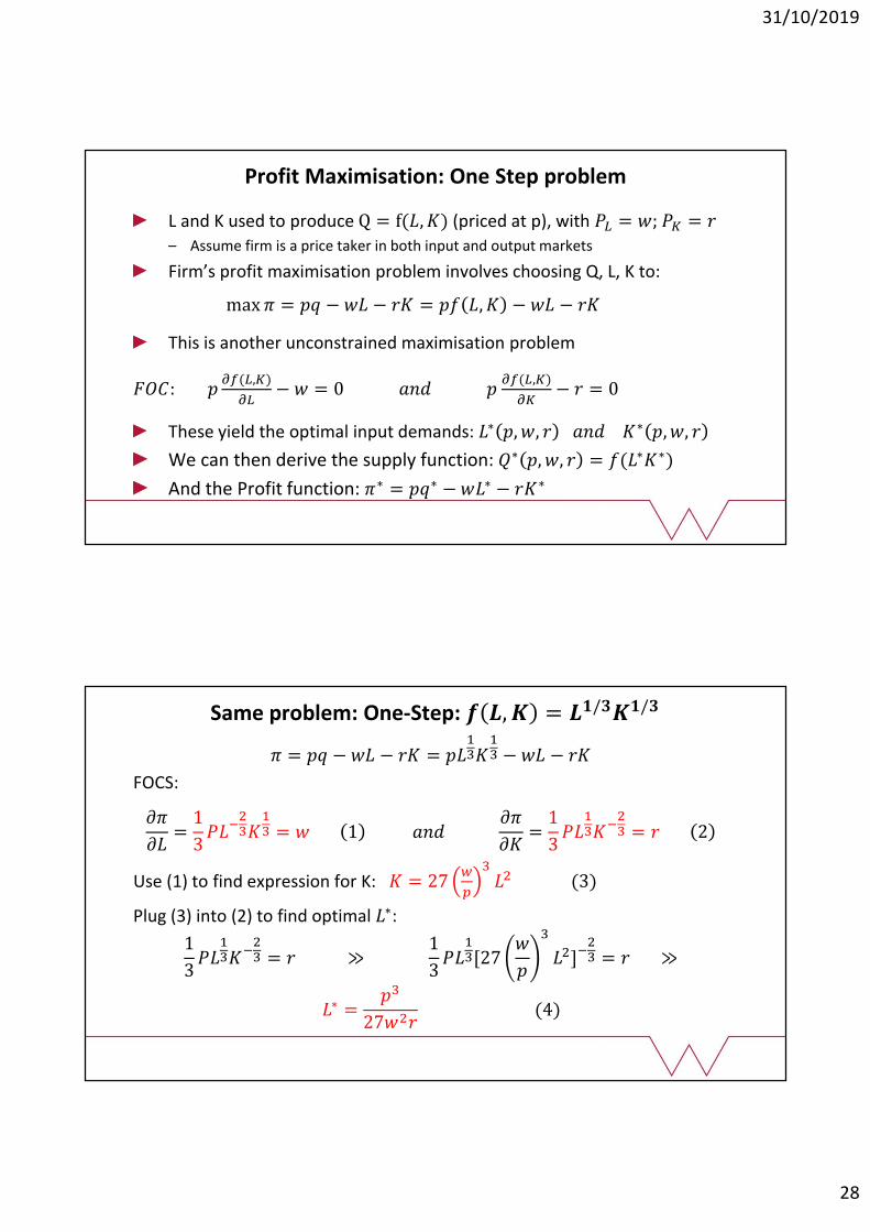
31/10/2019

28

Profit Maximisation: One Step problem

L and K used to produce Q = f(�, �) (priced at p), with �� = �; �� = �

– Assume firm is a price taker in both input and output markets

Firm’s profit maximisation problem involves choosing Q, L, K to:

max � = �� − �� − �� = �� �, � − �� − ��

This is another unconstrained maximisation problem

���: ���(�,�)

��− � = 0 ��� �

��(�,�)

��− � = 0

These yield the optimal input demands: �∗ �, �, � ��� �∗ �, �, �

We can then derive the supply function: �∗ �, �, � = �(�∗�∗)

And the Profit function: �∗ = ��∗ − ��∗ − ��∗

Same problem: One-Step: � �, � = ��/���/�

� = �� − �� − �� = �����

�� − �� − ��

FOCS:

��

��=

1

3���

���

�� = � 1 ���

��

��=

1

3��

����

�� = � 2

Use (1) to find expression for K: � = 27�

�

��� (3)

Plug (3) into (2) to find optimal �∗:

1

3��

����

�� = � ≫

1

3��

��[27

�

�

�

��]��� = � ≫

�∗ =��

27��� (4)

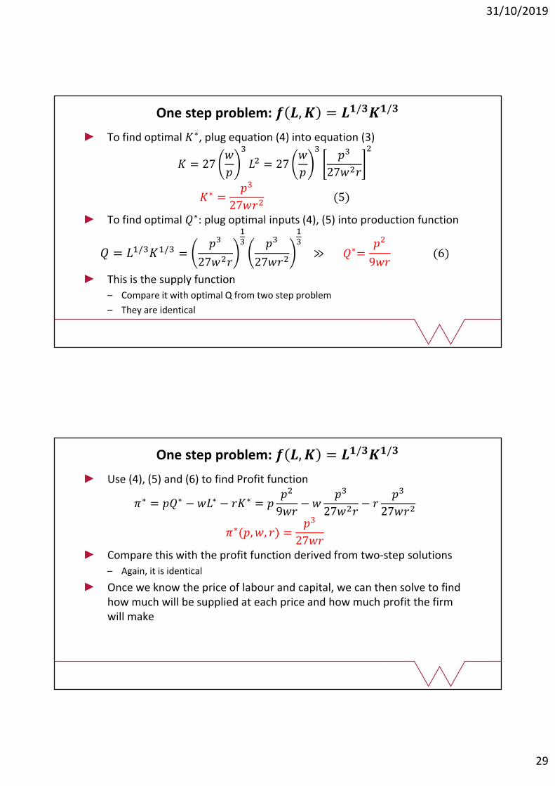
31/10/2019

29

One step problem: � �, � = ��/���/�

To find optimal �∗, plug equation (4) into equation (3)

� = 27�

�

�

�� = 27�

�

���

27���

�

�∗ =��

27��� (5)

To find optimal �∗: plug optimal inputs (4), (5) into production function

� = ��/���/� =��

27���

�� ��

27���

��

≫ �∗=��

9�� (6)

This is the supply function

– Compare it with optimal Q from two step problem

– They are identical

One step problem: � �, � = ��/���/�

Use (4), (5) and (6) to find Profit function

�∗ = ��∗ − ��∗ − ��∗ = ���

9��− �

��

27���− �

��

27���

�∗(�, �, �) =��

27��Compare this with the profit function derived from two-step solutions

– Again, it is identical

Once we know the price of labour and capital, we can then solve to find how much will be supplied at each price and how much profit the firm will make

31/10/2019

30

Profit and Supply Functions

Profit is maximised at Q* where:�� = ��

Profits are given by:� = ��∗ − � �∗

Total profit on top diagram is:� = �� − ��

Total profit on bottom diagram is:� = � − �� �∗ �∗

� �, �, � increases in p and decreases in w, r

� �, �, � is homogeneous of degree 1 in �, �, �

Profit functionTC(Q)TR=PQ

AC(Q)MC(Q)

T π

Quantity

Quantity

Price

Costs

Q*

Q*

�

P AR = MR

AC

�

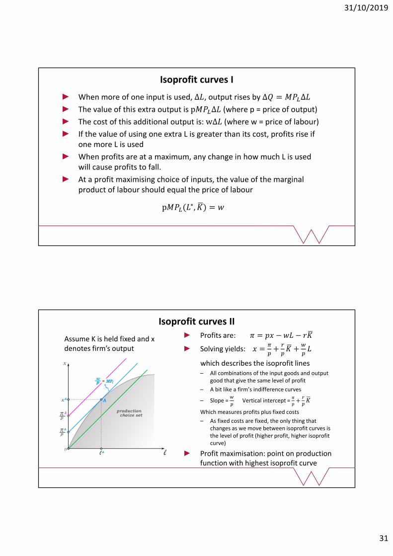
31/10/2019

31

Isoprofit curves I

When more of one input is used, ∆�, output rises by ∆� = ���∆�

The value of this extra output is p���∆� (where p = price of output)

The cost of this additional output is: w∆� (where w = price of labour)

If the value of using one extra L is greater than its cost, profits rise if one more L is used

When profits are at a maximum, any change in how much L is used will cause profits to fall.

At a profit maximising choice of inputs, the value of the marginal product of labour should equal the price of labour

p���(�∗, ��) = �

Profits are: � = �� − �� − ���

Solving yields: � =�

�+

�

��� +

�

��

which describes the isoprofit lines– All combinations of the input goods and output

good that give the same level of profit

– A bit like a firm’s indifference curves

– Slope = �

�Vertical intercept =

�

�+

�

���

Which measures profits plus fixed costs

– As fixed costs are fixed, the only thing that changes as we move between isoprofit curves is the level of profit (higher profit, higher isoprofitcurve)

Profit maximisation: point on production function with highest isoprofit curve

Isoprofit curves II

Assume K is held fixed and x denotes firm’s output

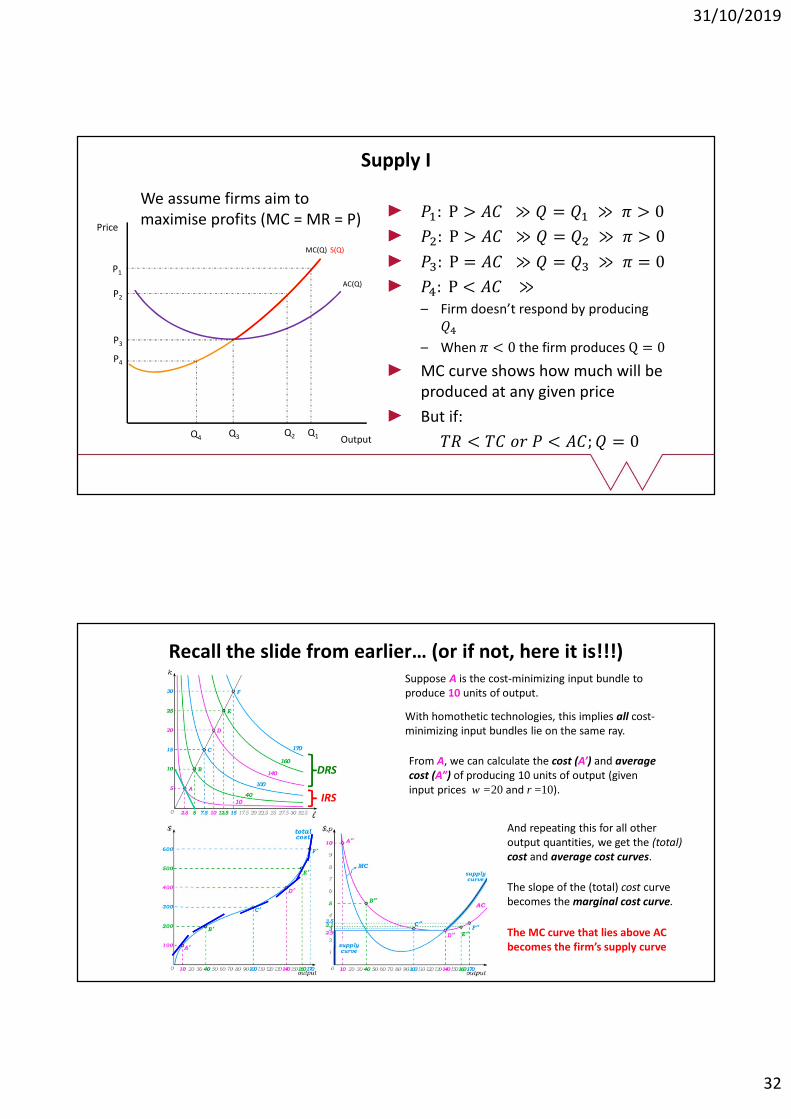
31/10/2019

32

Supply I

P2

P1

P4

Price

Output

P3

Q1Q2Q3Q4

��: P > �� ≫ � = �� ≫ � > 0

��: P > �� ≫ � = �� ≫ � > 0

��: P = �� ≫ � = �� ≫ � = 0

��: P < �� ≫– Firm doesn’t respond by producing

��

– When � < 0 the firm produces Q = 0

MC curve shows how much will be produced at any given price

But if:

�� < �� �� � < ��; � = 0

We assume firms aim to maximise profits (MC = MR = P)

MC(Q)

AC(Q)

S(Q)

Suppose A is the cost-minimizing input bundle to produce 10 units of output.

With homothetic technologies, this implies all cost-minimizing input bundles lie on the same ray.

IRS

DRSFrom A, we can calculate the cost (A’) and average cost (A”) of producing 10 units of output (given input prices w =20 and r =10).

And repeating this for all other output quantities, we get the (total) cost and average cost curves.

The slope of the (total) cost curve becomes the marginal cost curve.

Recall the slide from earlier… (or if not, here it is!!!)

The MC curve that lies above AC becomes the firm’s supply curve

31/10/2019

33

Supply II

Long run Supply (MC above AC)

Short run Supply (MC above AVC) - only needs to cover variable costs

Shape of supply depends on: shape of MC and whether there are FC

The supply function is homogeneous of degree 0 (in p, r, w)– If prices double, profit equation scales up, so optimal output is unaffected

Supply will slope upwards

Long run supply will be flatter than short run supply, due to fixed input, capital

Conclusion: Combining topics 1 and 2

In topic 1, we looked at the consumption decision– We derived consumer demand

In topic 2, we have considered the production decision– We have derived producer supply

We have seen that both the demand and supply functions depend on the market price of the good

Combining these theories allows us to understand the fundamental workings of a competitive market– The interaction between consumers and producers

– How equilibrium is determined in a market via the price mechanism which sends signals between the two sides