thermal and fluid design analysis of a square
TRANSCRIPT
THERMAL AND FLUID DESIGN ANALYSIS OF A SQUARE LATTICE HONEYCOMB NUCLEAR ROCKET ENGINE
By
JOHANN PLANCHER
A THESIS PRESENTED TO THE GRADUATE SCHOOL OF THE UNIVERSITY OF FLORIDA IN PARTIAL FULFILLMENT
OF THE REQUIREMENTS FOR THE DEGREE OF MASTER OF SCIENCE
UNIVERSITY OF FLORIDA
2002

Copyright 2000
by
Johann Plancher

To my Family

ACKNOWLEDGMENTS
This research would not have been possible without the contributions of several
people. I would like to thank Dr. Samim Anghaie for his support and his wise advice
throughout the duration of this project. His trust and guidance made my master’s degree
more than an academic experience. I also would like to express my thanks to Dr Edward
T. Dugan for his quality teaching and support throughout my graduate time at University
of Florida. I would also like to thank Dr. Darryl Butt for agreeing to take the time and
effort to be on my supervisory committee.
I would like to thank my parents and my brothers for their understanding and their
support. I would also like to express my thanks to the French team, all my friends in the
Department of Nuclear and Radiological Engineering and at INSPI who made me enjoy
my stay at the University of Florida. I am also grateful to Jennifer for her support and
encouragement, which helped me to complete this research.
iv

TABLE OF CONTENTS
page
ACKNOWLEDGMENTS ................................................................................................. iv
LIST OF TABLES............................................................................................................ vii
LIST OF FIGURES ......................................................................................................... viii
ABSTRACT........................................................................................................................ x
1 INTRODUCTION ............................................................................................................1
Nuclear Thermal Propulsion ........................................................................................... 1 History of the Nuclear Rocket Engine ............................................................................ 2 Work of the Thesis.......................................................................................................... 4
2 THERMAL HYDRAULIC DESIGN ANALYSIS OF THE SYSTEM OF THE NUCLEAR ROCKET ENGINE..........................................................................................6
System Description ......................................................................................................... 6 Concept of the Nuclear Thermal Propulsion (NTP) ................................................... 6 Thermal Hydraulic System ......................................................................................... 8 Reactor Core Design ................................................................................................... 9 Objective of the Calculation ..................................................................................... 12
Method of Analysis....................................................................................................... 17 Calculation Code....................................................................................................... 17 Variables of the System ............................................................................................ 19
3 IMPROVEMENT OF THE THERMAL HYDRAULIC PRE-CORE SYSTEM OF THE NUCLEAR ROCKET ENGINE...............................................................................21
Results and Discussion ................................................................................................. 21 Influence of the Turbine By-pass Fraction (TBP) .................................................... 21 Influence of the Reflector Flow Fraction (RFF) ....................................................... 23 Influence of the Direct Fraction................................................................................ 24 Comparison between “Parallel” and “Serial” System .............................................. 25 Comparison between “Full-topping” and “Bleed” Cycle System ............................ 27
Optimal Design of the Thermal Hydraulic System of the Nuclear Rocket Engine ...... 29
v

4 CORE HEAT TRANSFER ANALYSIS WITH FLUENT ............................................35
Description of the Problem ........................................................................................... 35 About Fluent ................................................................................................................. 37
General Overview ..................................................................................................... 37 Basic Physical Models .............................................................................................. 38 Heat Transfer Modeling on FLUENT....................................................................... 39 Turbulence Modeling on FLUENT .......................................................................... 41 Numerical Solvers..................................................................................................... 46
Definition of the Calculation ........................................................................................ 48 Dimensional parameters............................................................................................ 49 Gas Properties ........................................................................................................... 51 Boundary Conditions ................................................................................................ 53
5 EVALUATION OF THE CYLINDRICAL APPROXIMATION FOR A SQUARE MICROCHANNEL ...........................................................................................................55
Convergence of the Calculations .................................................................................. 55 Comparison between the Square and the Cylindrical Channel..................................... 58
Variation of the Outlet Velocity according to the Equivalent Diameter .................. 59 Variation of the Outlet Temperature according to the Equivalent Diameter............ 61 Variation of the Pressure Drop over 10 cm according to the Equivalent Diameter . 63 Variation of the Outlet Density according to the Equivalent Diameter.................... 65 Variation of the Temperature Difference between the Two Channel Types along the
Channel ..................................................................................................... 67 Observation on the Heat Transfer in the Channels ....................................................... 70
6 SUMMARY AND CONCLUSIONS .............................................................................75
LIST OF REFERENCES...................................................................................................78
BIOGRAPHICAL SKETCH .............................................................................................80
vi

LIST OF TABLES
Table Page 1 – Influence of the turbine by-pass fraction on the thermal hydraulic parameters in the
pre-core system ................................................................................................................31
2 – Influence of the reflector flow fraction on the thermal hydraulic parameters of the pre-core system with a “parallel” cooling........................................................................32
3 – Influence of the direct fraction on the thermal hydraulic parameters of the pre-core system with a “mixed” cooling ........................................................................................33
4 – Comparison of the highest pressure between the “parallel” and the “serial” systems.....34
5 – Comparison between a “full-topping” and a “bleed” cycle .............................................34
6 – Turbulence parameters for the two inlet velocities..........................................................45
7 – Reynolds number at the outlet (10 cm) for the two inlet velocities.................................69
vii

LIST OF FIGURES
Figure Page 1 – Nuclear rocket engine from Rover/NERVA Program.....................................................3
2 – Nuclear thermal propulsion rocket engine system...........................................................7
3 – Scheme of the pre-core system (TBP=Turbine By-Pass, RFF=Reflector Flow Fraction)...........................................................................................................................9
4 – Square Lattice Honeycomb Fuel Elements......................................................................10
5 – Moderated SLHC Reactor Core.......................................................................................11
6 – Schematic diagram of the parallel cooling system (INSPI model)..................................14
7 – Schematic diagram of the serial cooling system (NERVA model) .................................15
8 – Schematic diagram of the mixed cooling system ............................................................16
9 – Scheme of the main loop of the program code ................................................................19
10 – Turbine by-pass (TBP) fraction influence on the highest pressure and temperature of the pre-core system ..........................................................................................................22
11 – Reflector flow fraction (RFF) influence on the highest pressure and temperature of the pre-core system ..........................................................................................................23
12 – Direct fraction influence on the highest pressure and temperature of the pre-core system ..............................................................................................................................24
13 - Comparison of the “parallel” and the “serial” cooling system designs for different fuel wafer thickness .........................................................................................................25
14 – Comparison between a “full-topping” (bleed=0%) and a “bleed” cycle .......................27
15 – Comparison of the heat transfer to a fluid flowing through a cylindrical or a square micro channel...................................................................................................................36
16 – Axial Profile of the mesh used for FLUENT calculations.............................................49
viii

17 – Orthogonal profile of the mesh used for FLUENT calculations....................................50
18 – Fitting curve of the thermal conductivity of hydrogen ..................................................51
19 – Fitting curve of the viscosity of hydrogen .....................................................................52
20 – Fitting curve of the specific heat of hydrogen ...............................................................52
21 – Example of convergence of the results ..........................................................................56
22 – Enthalpy residual for the different calculations with Vi=20 m/s...................................57
23 – Enthalpy residual for the different calculations with Vi=100 m/s.................................57
24 – Average outlet velocity according to different hydraulic diameters (Vi=20 m/s) .........59
25 – Average outlet velocity according to different hydraulic diameters (Vi=100 m/s) .......60
26 – Average outlet temperature according to different hydraulic diameters (Vi=20 m/s)...61
27 – Average outlet temperature according to different hydraulic diameters (Vi=100 m/s).62
28 – Pressure drop according to different hydraulic diameters (Vi=20 m/s).........................63
29 – Pressure drop according to different hydraulic diameters (Vi=100 m/s).......................64
30 – Outlet density according to different hydraulic diameters (Vi=20 m/s) ........................65
31 – Outlet density according to different hydraulic diameters (Vi=100 m/s) ......................66
32 – Comparison of the thermal hydraulic parameters between the two types of channels (Vi=20 m/s)......................................................................................................................67
33 – Comparison of the thermal hydraulic parameters between the two types of channels (Vi=100 m/s)....................................................................................................................68
34 – Velocity orthogonal distribution of the 1 mm square channel after 10 cm ...................70
35 – Velocity orthogonal distribution of the 10 mm square channel after 10 cm .................71
36 – Temperature orthogonal distribution of the 1 mm square channel after 10 cm.............72
37 – Temperature orthogonal distribution of the 10 mm square channel after 10 cm...........72
ix

Abstract of Thesis Presented to the Graduate School
of the University of Florida in Partial Fulfillment of the Requirements for the Degree of Master of Science
THERMAL AND FLUID DESIGN ANALYSIS OF A SQUARE LATTICE HONEYCOMB NUCLEAR ROCKET ENGINE
By
Johann Plancher
May 2002 Chairman: Professor Samim Anghaie Major Department: Nuclear and Radiological Engineering
Nuclear thermal propulsion is a prime system for handling the high requirements
of the future spatial missions to Mars. The Innovative Nuclear Space Power and
Propulsion Institute (INSPI) has developed a nuclear rocket engine design based on a
square lattice honeycomb core. This work focuses on the pre-core system of the rocket
engine bringing hydrogen coolant to the core at the proper thermal hydraulic conditions.
In order to minimize the thermal and physical stresses on the system, calculations are
performed using a nuclear thermal rocket engineering simulation computer code.
Different variables of the system are evaluated to minimize the thermal and mechanical
stresses on the system. It appears that the optimized design, similar to the Rover/NERVA
Program’s design, presents a serial cooling of the exhaustion nozzle of the rocket and
then the core reflector structure, with a minimum turbine by-pass ratio of 10%. However
if parallel cooling of the nozzle and reflector is chosen instead, then the reflector flow
fraction is 35%.
x
In a second part, a specific issue of the heat transfer in the core is analyzed. The
simulation code used to perform the design analysis of the system approximates the
square channels of the core to cylindrical channels. It appears, according to the
calculations performed on FLUENT, that this approximation brings a significant error for
hydraulic diameter lower than 3 mm. This difference might come from the effect of the
corners of the square channel on the heat transfer. We should consider modeling the
square channels as cylindrical channels with the diameter slightly higher than the
equivalent hydraulic diameter.
xi

CHAPTER 1 INTRODUCTION
The idea of a nuclear rocket engine has been around for over 40 years. Before
presenting the work of this thesis, the basics of the nuclear space propulsion and its origin
are rapidly discussed to show the importance of this field in the future of science.
Nuclear Thermal Propulsion
Nuclear thermal propulsion (NTP) is a relatively simple concept. Compared to
chemical concepts, it provides higher specific impulse, ISP, which represents the ratio of
the thrust over the rate of fuel consumption. A chemical rocket uses the heat produced by
burning fuel and oxidizer in a thrust chamber. In the case of a nuclear rocket engine the
heat is generated in a nuclear reactor core by a controlled nuclear fission reaction. The
energy produced by the reactor is carried away by hydrogen, which plays the role of
coolant or propellant. This high temperature gas is then exhausted through a nozzle
producing a massive thrust.
In the case of chemical rockets, the process needs a huge amount of fuel to power
the rocket over long distances. For many years, this concept has been used to launch
rockets from the earth allowing high thrust in a short period of time. But when
considering the objectives of the next spatial missions, nuclear propulsion meets the
requirements. After the past exploration of the near environment of the earth, the
objectives are now to go further into space with the focus on Mars and other
interplanetary missions for the next decades. These missions will be longer than usual
1

2
ones and thus will be exposed to greater amounts of radiation in space. This must be
taken into consideration. For manned missions, the travel time needs to be reduced and
only the NTP concept is conceivable. NTP is two to three times more efficient than the
chemical concept considering its ISP.
nconsumptiofuelofratethrustISP ___
�
Considering missions to Mars, a nuclear propulsion rocket would reduce the
travel time to 300 days, instead of 600 days with a chemical rocket.
History of the Nuclear Rocket Engine
The United States embarked on a program to develop nuclear rocket engines in
1955. In the 60s, this program became the project Rover/NERVA (Nuclear Engine for
Rocket Vehicle Applications). Initially nuclear rockets were considered as a potential
backup for international ballistic missile propulsion but later proposed applications
included both a lunar second stage as well as use in manned-Mars flight.
Under the Rover/NERVA program, 19 different reactors were built and tested
during the period of 1959-1969. Additionally, several cold flow (non-fueled) reactors
were tested as well as a nuclear fuels test cell. Figure 1 shows a photo of a nuclear rocket
engine designed and tested. The Rover/NERVA program was terminated in 1973, due to
budget constraints and an evolving political climate. The Rover/NERVA program would
have led to the development of a flight engine had the program continued through a
logical continuation. The Rover/NERVA program was responsible for a huge number of
technological achievements.

3
Figure 1 – Nuclear rocket engine from Rover/NERVA Program
In the late 1980s, mandated by President George Bush, the Space Exploration
Initiative (SEI) envisioned a return to the Moon, this time to stay, and subsequently, a
manned expedition to Mars. For a manned-Mars expedition, the trip time must be as short
as possible to assure the survival of the astronauts. Such things as exposure to cosmic
radiations, bone decalcification, and muscle atrophy are of great concern. Short time trip
dictates the use of nuclear propulsion, allowing the one-way trip to be made in roughly 4
months (Finseth, 1991). This program was stopped in 1992 under Clinton administration.

4
Today an extensive amount of research is being conducted to set-up a rocket
design using nuclear energy. NTP is one of the many ways to use the energy provided by
nuclear fission. Other research focuses on an indirect use of the nuclear energy. The
Innovative Space Power and Propulsion Institute (INSPI) based on campus at University
of Florida designed a NTP rocket engine in cooperation with the NASA Marshall Space
Center. Much work has already been completed; yet further analyses are still needed to
confirm the potential of this system. J. Given (1993) performed a core analysis of the
nuclear rocket reactor determining the main parameters of the core. This work constitutes
an advanced analysis of the thermal system of the nuclear rocket engine.
Work of the Thesis
The purpose of this work is to analyze the thermal hydraulic system of the nuclear
rocket engine, to improve its characteristic and find its limits for further uses. In the first
part described in Chapters 2 and 3, the thermal hydraulic system of the nuclear rocket
engine is analyzed using the simulation code developed at INSPI by S. Anghaie (Anghaie
& Chen, 1998). This code allows modifications of the main variables of the pre-core
system. The influence of these variables is studied to optimize the pre-core system. INSPI
and NERVA pre-core systems are compared. An optimal system is proposed from this
analysis.
The second part (Chapters 4 and 5) focuses on a specific issue of the INSPI
nuclear rocket engine. The heat transfer in the micro-channels of the core is specific
because of the high temperature, the high pressure and the unusual geometry. To model
the heat transfer in these square micro-channels of the core, the simulation code uses
correlations for cylindrical channels, considering the hydraulic diameter of the square

5
channels. However according to the specificity of the heat transfer, the hydraulic
diameter approximation might be inaccurate. The computational fluid dynamics (CFD)
code FLUENT is used to do a qualitative study of this approximation. Thanks to these
calculations, some improvement can be done on the nuclear rocket engine simulation
code.

CHAPTER 2 THERMAL HYDRAULIC DESIGN ANALYSIS OF THE SYSTEM OF THE
NUCLEAR ROCKET ENGINE
This chapter presents the calculations performed to optimize the thermal hydraulic
system of the nuclear rocket engine. The results are discussed in the following chapter.
After a description of the system of the nuclear rocket engine, the method of calculation
used in this first part will be presented.
System Description
Much research has been done on various systems using nuclear energy as the
main source for the rocket thrust. This energy can be used directly or indirectly. NTP is a
direct approach.
Concept of the Nuclear Thermal Propulsion (NTP)
The nuclear thermal propulsion (NTP) concept is relatively simple and provides
higher specific impulse ISP than chemical concepts. A NTP rocket engine uses fission
energy instead of combustion energy for a chemical rocket. Figure 2 presents a simple
scheme of a nuclear rocket engine using NTP. The energy produced by the reactor is
carried away by hydrogen, which plays the role of coolant or propellant. The exhaustion
of this high temperature gas through a nozzle produces a massive thrust for a relatively
small core. The NTP concept is two to three times more efficient than the chemical
concept used today due to its high ISP.
When considering the objectives of the next spatial missions, NTP reaches the
high requirements for long travel. Using NTP decreases the mass of the rocket. It does
not require a huge amount of fuel compared to a chemical rocket. The NTP concept also 6

7
reduces the travel time and the radiation amount received during this travel, which makes
it possible to plan Mars manned missions in the future.
Figure 2 – Nuclear thermal propulsion rocket engine system
This work presents an analysis of the nuclear rocket engine concept being
developed at University of Florida’s INSPI. The system uses NTP to power the rocket.
Calculations showed that this type of rocket could reach very high thrust for a long period
of time with a high power to weight ratio. INSPI developed a new design for NTP rocket
8
engine named “Square Lattice Honeycomb Core” (SLHC) nuclear rocket engine. The
main aspects of this system are presented in the following sections.
Thermal Hydraulic System
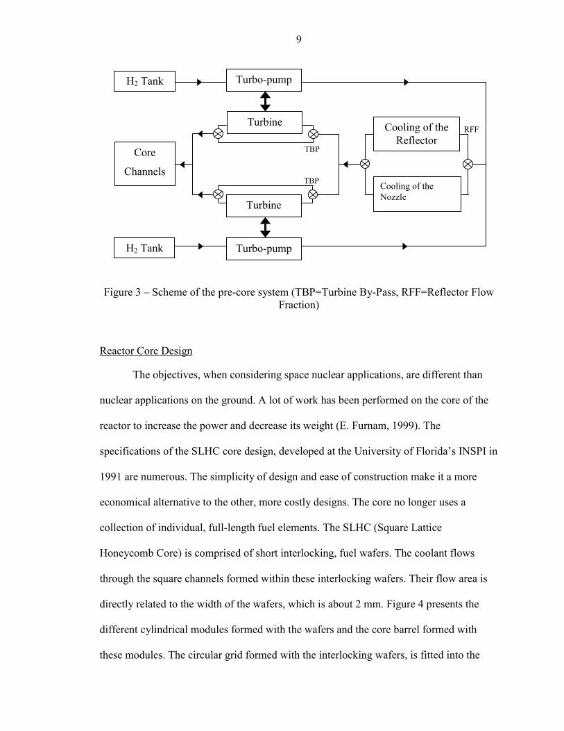
A schematic diagram of the pre-core system configuration is shown in Figure 3.
The main aspects of the core design are its square lattice honeycomb structure allowing a
better heat exchange with the coolant, the high temperature material of the core, and the
simplicity of the thermal hydraulic system. The hydrogen coolant is released as a gas
from the tank and goes through a turbo-pump, which increases its pressure. Then the
hydrogen is preheated in the nozzle and in the reflector, which are both cooled down by
the flowing hydrogen, in order to preserve their structure. The preheated hydrogen drives
a turbine, which powers the initial turbo-pump. After this pre-processing, the hydrogen
arrives in the core at a low temperature. The coolant goes through the square lattice
honeycomb core by several rectangular micro-channels and is heated to very high
temperatures. This heating increases the velocity of the gas, while its pressure and its
density decrease. The gas enters the thrust chamber at high velocity, temperature and
pressure. The exhaustion of the hydrogen through the nozzle creates a massive thrust.
9
RFF
TBP
TBP Cooling of the Nozzle
Cooling of the Reflector
Turbine
Core
Channels
Turbo-pump
Turbine
H2 Tank
H2 Tank
Turbo-pump
Figure 3 – Scheme of the pre-core system (TBP=Turbine By-Pass, RFF=Reflector Flow Fraction)
Reactor Core Design
The objectives, when considering space nuclear applications, are different than
nuclear applications on the ground. A lot of work has been performed on the core of the
reactor to increase the power and decrease its weight (E. Furnam, 1999). The
specifications of the SLHC core design, developed at the University of Florida’s INSPI in
1991 are numerous. The simplicity of design and ease of construction make it a more
economical alternative to the other, more costly designs. The core no longer uses a
collection of individual, full-length fuel elements. The SLHC (Square Lattice
Honeycomb Core) is comprised of short interlocking, fuel wafers. The coolant flows
through the square channels formed within these interlocking wafers. Their flow area is
directly related to the width of the wafers, which is about 2 mm. Figure 4 presents the
different cylindrical modules formed with the wafers and the core barrel formed with
these modules. The circular grid formed with the interlocking wafers, is fitted into the

10
graphite shroud. This grid-shroud combination serves as a support mechanism against
axial forces. Six of these grid-shroud modules are stacked on top of each other to form a
complete length of the core.
1 to 3 mm
Figure 4 – Square Lattice Honeycomb Fuel Elements
The use of stacked grid-shroud fuel modules provides added fuel temperature
control by manipulation of the power shape. The power shape or power distribution
within the core can be manipulated by loading each module with different concentrations
of uranium. For example, placing high enrichment modules on the top and bottom of the
11
stack can flatten the core’s axial power shape. Since the power distribution is directly
related to the heat flux, a flattened power shape insures that the whole length of the core
is operating at its highest and most efficient temperature.
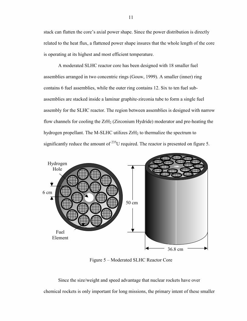
A moderated SLHC reactor core has been designed with 18 smaller fuel
assemblies arranged in two concentric rings (Gouw, 1999). A smaller (inner) ring
contains 6 fuel assemblies, while the outer ring contains 12. Six to ten fuel sub-
assemblies are stacked inside a laminar graphite-zirconia tube to form a single fuel
assembly for the SLHC reactor. The region between assemblies is designed with narrow
flow channels for cooling the ZrH2 (Zirconium Hydride) moderator and pre-heating the
hydrogen propellant. The M-SLHC utilizes ZrH2 to thermalize the spectrum to
significantly reduce the amount of 235U required. The reactor is presented on figure 5.
36.8 cm
50 cm
Fuel Element
Hydrogen Hole
6 cm
Figure 5 – Moderated SLHC Reactor Core
Since the size/weight and speed advantage that nuclear rockets have over
chemical rockets is only important for long missions, the primary intent of these smaller

12
rocket engines is to power interplanetary spacecraft. These rockets will be used after the
craft has escaped Earth’s gravitational pull. Then considerably less thrust is required from
these rockets than those used in the Saturn V or main booster rockets of the Space
Shuttle. Only tens-of-thousands of pounds of thrust is expected from these rockets,
whereas the main booster rockets for terrestrial launches produce thrust in the millions of
pounds. Therefore, the rockets studied in this paper are expected to produce between
10,000 lbf and 50,000 lbf thrust without exceeding the temperature limitations of the fuel.
To obtain such performance, the core uses new materials. Similar to
Rover/NERVA reactors, the core is fueled with 93% enriched uranium. Materials
considered for this reactors are tri-carbide solid solution fuels like (U,Zr,Nb)C or
(U,Zr,Ta)C, which have proven to be efficient at high temperatures. High melting point
and high thermal conductivity are notably two main characteristics of these ultrahigh
temperature materials (Anghaie, Knight, Gouw & Furnam, 2001).
Objective of the Calculation
Calculations on the core design have already been performed (Anghaie, Knight,
Gouw & Furnam, 2001). These new calculations focus on optimizing the pre-core
system. The goal of the pre-core system is to bring the hydrogen to the core at the proper
conditions of pressure and temperature as well as to limit the thermal stresses and
pressure drops in the system. As presented on Figure 6, 7, and 8 various pre-core systems
are studied. These systems correspond to different pre-heating of the coolant hydrogen,
defined by some variables:
�� Figure 6 – INSPI model: This design considers a parallel cooling of the reflector and the nozzle. The main variables are the turbine by-pass ratio (TBP), which defines the fraction of flow not going through the turbine and the reflector flow fraction (RFF), which defines the fraction of the flow cooling the reflector.

13
�� Figure 7 – NERVA model: This design considers a serial cooling of first the nozzle and then the reflector. The main variable is the TBP.
�� Figure 8 – Mixed model: This design considers a mixed cooling of the reflector and the nozzle. A fraction of the flow called the Direct Fraction goes directly to the reflector. The other part of the flow goes first through the nozzle and then through the reflector as in the serial system.
Thermal hydraulic calculations are performed to study the influence of the main
variables that determine the efficiency of the pre-core system. An optimized pre-core
system is given as a result.

14
Figure 6 – Schematic di
TBP
Cooling of the Nozzle
Cooling of the Reflector
agram of the parallel co
TBP
RFF
oling system (INS
RFF
RFFPI model)

15
Cthe
Figure 7 – Schematic dia
TBP
Coolithe N
ooling of Reflector
gram of the serial cooli
TBP
ng of ozzle
ng system (NERVA model)

16
le
Direct Fraction
Cooling of the Reflector
Cooling of the Nozz
Figure 8 – Schematic diagram of the mixed cooling syst
Direct
DirectTBP
TBPem

17
Method of Analysis
The following paragraph presents the method used to analyze the nuclear rocket
engine system. First, the simulation code used to perform calculations on the system is
presented. Secondly, we will see the modification done on this code to analyze the
influence of the different variable of the system.
Calculation Code
A nuclear thermal rocket engineering simulation computer code (Anghaie &
Given, 1997) is used to perform thermal hydraulic design analysis for the SLHC nuclear
thermal rocket system. The original model simulates a full-toping expander cycle engine
system and the thermal fluid dynamics of the core coolant flow. The system simulation
code was originally developed for analysis of NERVA-Derivative and Pratt&Whitney
XNR-2000 nuclear thermal rockets. The code was modified and adapted to the square
lattice geometry of the fuel design. It notably uses a cylindrical approximation for the
square micro channels, which will be discussed in the Chapters 4 and 5 of this work. The
code is composed of different sub-routines, which can be modified to analyze various
system designs. The calculations are iterative and converge to the solutions of the main
parameters of the system for specified exhaustion chamber conditions. Considering the
same operating conditions, the variables of the pre-core system are modified in the sub-
routines of the code, to find the optimal thermal parameters in the system. The original
system is modified to obtain an optimized system with the optimal variables.
The code simulates a complete nuclear rocket engine system, however the
calculations are separated according to the different components of the system in several
sub-routines. These sub-routines are linked to perform a steady state system analysis at
any desired operating conditions. The user defines these conditions of the rocket engine:

18
thrust chamber pressure, thrust chamber temperature, and rocket thrust. Then the
programs of the code calculate by iterations the mass flow rate, pump pressure rise, and
core thermal power needed to produce the desired operating conditions.
Figure 9 presents the main loop on the pre-core thermal hydraulic system. It
shows the main parameters of this iteration and the sub-routines requested in the main
loop. The goal of this figure is not to explain the complete program, which is made of
numerous sub-routines, but it is useful to understand the method of calculation used in
the code and see how the variables influence the calculations.
There are two types of modifications. First the main variables of the system are
changed: RFF, TBP. Secondly the main loop structure is changed to obtain “parallel”,
“serial” or “mixed” systems. Several combinations of these variables are tested and
discussed. The bleed percentage, which characterizes the leaking after the turbine, is set
to zero to model a “full-topping” cycle. In a final analysis, this percentage is varied to
see its influence on the system.

19
Main Parameters of the loop
Bleed percentage: Bleed
Turbine by-pass ratio: TBP
Reflector flow fraction: RCRFF
Total mass flow rate: W
Turbine mass flow rate (half of system): )1()1(2
TBPBleed
WWturb ��
��
�
Reflector cooling mass flow rate: RCRFFBleedWWrcr �
�
�
1
Nozzle cooling mass flow rate: )1(1
RCRFFBleedWWrcr ��
�
�
Iteration on the main loop (till convergence of the results)
TPUMP (P00, T00,…., P01, T01,….) Turbo-pump Sub-routine
P02 = P01 & T02 = T01
RCNOZZLE (P02, T02,…., P03, T03,….) Nozzle cooling Sub-routine
P04 = P01 & T04 = T01
RCREFLECT (P04, T04,…., P05, T05,….) Reflector cooling Sub-routine
MIXER (P03, T03, Wrcn, P05, T05, Wrcr, P06, T06)
TURBINE (P06, T06, Wturb,…., P07, T07) Turbine Sub-routine
MIXER (P06, T06, Wturb*TBP, P07, T07, Wturb, P08, T08)
CORE (P08, T08,……) Core Sub-routine
Figure 9 – Scheme of the main loop of the program code
Variables of the System
The main variables analyzed for the SLHC rocket engine system are the turbine
by-pass fraction (TBP), the reflector flow fraction (RFF) and the direct fraction, which
are specified on Figure 6, 7, and 8 for the different systems. The TBP concerns the

20
fraction of the coolant flow, which does not go through the turbine but goes directly to
the core. The fraction going through the turbine needs to be high enough to drive the
rotation of the turbine within limits due to safety issues.
The other two variables deal with the cooling of the nozzle and the reflector. At
the same time the coolant is heated up, and this heat is used to drive a turbine, which
powers the initial turbo-pump. The structure of these two elements needs to be cooled
down to avoid high thermal stress. The different cooling systems studied in this work are:
�� “Serial” cooling system: the coolant goes through the nozzle and afterwards through the reflector,
�� “Parallel” cooling system: the coolant flow is separated, one part flowing through the reflector, the other part through the nozzle and,
�� “Mixed” cooling system: a part of the coolant flow goes directly to the reflector and the other goes first through the nozzle and afterwards through the reflector.
The “serial” system design is similar to the NERVA system design made in the
60s. The “parallel” system design is defined by the RFF, which determines the fraction of
the coolant flow for these two elements. The “mixed” system is determined by the direct
fraction of the flow, which goes directly through the reflector without going through the
nozzle. These systems are presented in Figure 6, 7, and 8.
All the systems previously presented are full-topping expander cycle systems: all
of the propellant is exhausted through the nozzle at the core exit temperature. An
alternative to this system is the “bleed” cycle where a part of the flow is expulsed out
after being through the turbine. Comparison with this type of cycle is also presented in
order to discuss the efficiency of a “full-topping” cycle. A leakage in the coolant flow
after the turbine is modeled with the bleed variable, which represents the fraction of flow
that leaks out in the turbine.

CHAPTER 3 IMPROVEMENT OF THE THERMAL HYDRAULIC PRE-CORE SYSTEM OF THE
NUCLEAR ROCKET ENGINE
This chapter presents and discusses the results of the first part calculations. Three
main variables of a full-topping system are analyzed. A comparison between a bleed
cycle and a full-topping cycle is also presented.
Results and Discussion
For all the calculations performed in this study operating conditions are kept
constant: requested thrust 30,000 lbf, expansion chamber entrance conditions at 3000 K
and 1000 psi. The fuel wafer thickness, which is the other entry for the code, is taken at
an average value of 1.5 mm for most calculations. The “parallel – serial” comparison is
performed according to different wafer thickness. For the other calculations, the highest
temperature and pressure in the pre-core system are used to evaluate the different designs.
The goal is to have for the same operating conditions, the lowest “highest pressure and
highest temperature”, to minimize the pressure drop and the thermal stress in the pre-core
system.
Influence of the Turbine By-pass Fraction (TBP)
The first results concern the turbine by-pass fraction (TBP). The general influence
of this fraction on the system is studied for the parallel cooling system, but can be
qualitatively considered for other systems. The results are presented in Table 1 at the end
of this chapter. The focus was put on the highest temperature and pressure in the pre-core
system, which represent the thermal and mechanical stresses. The goal of optimizing the
21

22
variables is to minimize the macroscopic stresses on the structure of the rocket. The
highest temperature corresponds to the temperature at the reflector outlet. The highest
pressure corresponds to the pressure at the turbo-pump outlet. Figure 10 shows that the
TBP fraction has no influence on the highest temperature. It also shows that the lower
this fraction is, the lower the peak pressure is. However the TBP has a lower safety limit
of about 10%. This by-pass is a safety guaranty. In case the turbine is blocked, the flow
will still be ejected, going through this by-pass. Therefore considering these results, an
appropriate value for the TBP would be around 10%.
1950
2000
2050
2100
2150
2200
2250
2300
2350
5% 10% 15% 20% 25% 30%
Turbine by-pass fraction (flow %)
Hig
hest
Pre
ssur
e (p
si)
250
255
260
265
270
275
280
285
290
Hig
hest
tem
pera
ture
(K)
HighestPressureHighestTemperature
Optimum Value
Figure 10 – Turbine by-pass (TBP) fraction influence on the highest pressure and temperature of the pre-core system

23
Influence of the Reflector Flow Fraction (RFF)
The second variable studied for a “parallel” cooling system is the RFF. This
variable is the fraction of the flow going through the reflector structure. The results are
presented at the end of this chapter on Table 2. The highest temperature and pressure
points are respectively the reflector outlet and the turbo-pump outlet. The influence of
this variable is shown in Figure 11. It appears that to minimize the pressure drop and the
temperatures, this fraction needs to be set at in a range of 30 to 40 %. For RFF equal to
35%, the highest pressure is under 2000 psi and the highest temperature under 300 K,
which are good values in order to relatively reduce the thermal and mechanical stresses.
The mechanical stress is the greatest concerns, however the thermal stress must not be
neglected.
1800
1900
2000
2100
2200
2300
2400
2500
2600
2700
2800
10% 20% 30% 40% 50% 60% 70%
Reflector flow fraction (flow %)
Hig
hest
pre
ssur
e (p
si)
0
100
200
300
400
500
600
700
800
900
1000
Hig
hest
tem
pera
ture
(K)
HighestPressureHighestTemperature
Optimum Value
Figure 11 – Reflector flow fraction (RFF) influence on the highest pressure and temperature of the pre-core system

24
Influence of the Direct Fraction
By varying the direct fraction, we can study different systems, called “mixed”
cooling systems. One part of the flow goes directly through the reflector, the other part
goes through the nozzle first and then through the reflector. When the direct fraction is
close to zero, the system is then called “serial” systems corresponding to the type of the
NERVA design. Results presented on Table 3 and plotted on Figure 12 show the
influence of this fraction on the main stress parameters. It appears that the lower the
direct fraction, the better the design. The NERVA design type or “serial” system, which
corresponds to a direct fraction close to zero, presents the best thermal hydraulic
parameters.
1800
1900
2000
2100
2200
2300
2400
2500
2600
2700
2800
2900
0 10 20 30 40 50 60 70
Direct fraction (flow %)
Hig
hest
pre
ssur
e (p
si)
0
50
100
150
200
250
300
350
400
450
500
550
Hig
hest
tem
pera
ture
(K)
Highest Pressure
Highest Temperature
Figure 12 – Direct fraction influence on the highest pressure and temperature of the pre-
core system
25
Comparison between “Parallel” and “Serial” System
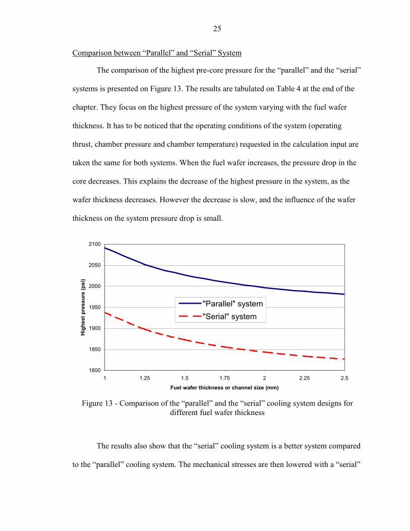
The comparison of the highest pre-core pressure for the “parallel” and the “serial”
systems is presented on Figure 13. The results are tabulated on Table 4 at the end of the
chapter. They focus on the highest pressure of the system varying with the fuel wafer
thickness. It has to be noticed that the operating conditions of the system (operating
thrust, chamber pressure and chamber temperature) requested in the calculation input are
taken the same for both systems. When the fuel wafer increases, the pressure drop in the
core decreases. This explains the decrease of the highest pressure in the system, as the
wafer thickness decreases. However the decrease is slow, and the influence of the wafer
thickness on the system pressure drop is small.
1800
1850
1900
1950
2000
2050
2100
1 1.25 1.5 1.75 2 2.25 2.
Fuel wafer thickness or channel size (mm)
Hig
hest
pre
ssur
e (p
si)
5
"Parallel" system"Serial" system
Figure 13 - Comparison of the “parallel” and the “serial” cooling system designs for
different fuel wafer thickness
The results also show that the “serial” cooling system is a better system compared
to the “parallel” cooling system. The mechanical stresses are then lowered with a “serial”

26
cooling. Moreover the parallel system requires mixers to mix the different separated
flows, which are at different temperature and pressure conditions. These mixers could
present a technical problem due to the specific thermal hydraulic conditions of the
system. Then it is easier to avoid separating and recombining cooling flows. Considering
these aspects, the “serial” cooling system is the best concept.

27
Comparison between “Full-topping” and “Bleed” Cycle System
The “bleed” cycle considers a leakage of the flow in the turbine. To model this
cycle, a modification has been done in the mass flow rate calculation. A variable called
the “bleed” percentage defines the percentage of flow lost in the turbine. This variable is
modified in the code considering a “serial” system, to see its influence on the thermal
hydraulic parameters of the system. Again the focus is put on the highest pressure and the
highest temperature in the pre-core system, which evaluates the thermal and mechanical
stress on the structure. Figure 14 presents the influence of this variable on the thermal
hydraulic parameters.
1840
1845
1850
1855
1860
1865
1870
1875
1880
0 5 10 15 20 25 30Bleed Percentage (%)
Hig
hest
Pre
ssur
e (p
si)
160
165
170
175
180
185
190
195
200
Hig
hest
Tem
pera
ture
(K)
Highest Pressure
HighestTemperature
Figure 14 – Comparison between a “full-topping” (bleed=0%) and a “bleed” cycle
When the “bleed” percentage is zero the system represented is a “full-topping”
cycle. The same operating conditions are considered for all the calculations. Then to
obtain the same mass flow rate in the chamber, the initial mass flow rate is bigger due to

28
the loss in the turbine. This means that as the bleed percentage increases the consumption
of coolant increases for the same operating conditions. As we see on the plot the highest
temperature decreases with this variable. In fact the mass flow rate is bigger in the nozzle
and the reflector, because of the loss in the turbine. Then the cooling is more efficient and
the coolant temperature does not rise as much as for a normal flow rate. However the
increase of the variable makes the highest pressure of the system increase too. As we
want to minimize the pressure drop in the system, it appears that the “full-topping” cycle
system is optimum. However a 5% bleed percentage does not bring a big increase in the
pressure. In this case, the loss of coolant is more an issue than the increase of pressure.
29
Optimal Design of the Thermal Hydraulic System of the Nuclear Rocket Engine
The calculations made on the simulation code elaborated at INSPI on the system
of nuclear rocket engine show that the organization of the pre-core system greatly
influences the thermal hydraulic parameters. To minimize the pressure drops and the
temperature high in the system while keeping the same thrust for the rocket, the optimum
system design appears to be the full-topping “serial” system or NERVA design type, with
a turbine by-pass fraction of about 10%. This system uses a serial cooling system, which
avoids mixing of different coolant flows. However if a “parallel” system was considered
then the reflector flow fraction, which characterizes the separation of the cooling, should
to be set at about 35%, to obtain an optimum system.
When considering an optimized system not only the design, but also the
feasibility of this design has to be considered. Considering the parallel system, it might be
a technical issue to built efficient mixers, which would mix two incoming flows at
different temperature and pressure.
If a “bleed” cycle is considered instead of a “full-topping” cycle, then the fraction
of the flow leaking out after the turbine should be minimum. Maintaining the same
operating conditions, the increase of this fraction makes decrease the highest temperature
value in the pre-core system. In fact the cooling is better, but the mass flow rate is much
higher, a part of the flow leaking out of the cycle before entering the core.
All the results from the calculations are presented on the following tables:
�� Table 1 presents the influence of the TBP on the thermal hydraulic parameters at the main points of the pre-core system. Figure 10, previously presented in this chapter, uses the values for the highest pressure and temperature points, which are respectively the “turbo-pump outlet” and the “reflector outlet”.

30
�� Table 2 presents the influence of the RFF on the thermal hydraulic parameters at the main points of the pre-core system with “parallel” cooling. Figure 11, previously presented in this chapter uses the values for the highest pressure and temperature points, which are respectively the “turbo-pump outlet” and the “reflector outlet”.
�� Table 3 presents the influence of the direct fraction on the thermal hydraulic parameters at the main points of the pre-core system. Figure 12, previously presented in this chapter, uses the values for the highest pressure and temperature points, which are respectively the “turbo-pump outlet” and the “nozzle outlet”.
�� Table 4 presents a comparison between the “parallel” and the “serial” cooling systems for different wafer thickness based on the highest pressure in the pre-core system. These results were presented on figure 13.
�� Table 5 presents a comparison between a “full-topping” and a “bleed” cycle based the mass flow rate, the highest pressure and temperature of the pre-core system. These results were previously presented on figure 14.

31
Table 1 – Influence of the turbine by-pass fraction on the thermal hydraulic parameters in the pre-core system
Turbine by-pass Ratio 5% 10% 15% 20% 25% 30%
T (K) 35 36 36 36 37 38 Point 1 Turbo-pump Outlet (Highest Pressure) P (psi) 1988 2028 2076 2138 2220 2334
T (K) 264 264 264 265 265 265 Point 2 Reflector Outlet
(Highest Temperature) P (psi) 1986 2026 2075 2137 2218 2332
T (K) 185 185 186 186 187 188 Point 3 Nozzle Outlet P (psi) 1471 1509 1556 1616 1695 1805
T (K) 216 216 217 217 218 218 Point 4 Turbine Inlet P (psi) 1471 1509 1556 1616 1695 1805
T (K) 200 200 200 199 199 198 Point 5 Core Inlet P (psi) 1060 1060 1060 1060 1060 1060

32
Table 2 – Influence of the reflector flow fraction on the thermal hydraulic parameters of the pre-core system with a “parallel” cooling
Reflector Flow Fraction 10% 20% 30% 35% 40% 45% 50% 60% 70%
T(K) 34 35 35 35 36 36 36 38 39 Point 1 Turbo-pump
Outlet Highest Pressure P(psi) 1837 1881 1940 1979 2028 2087 2161 2373 2735
T(K) 958 496 341 297 264 239 218 189 168 Point 2 Reflector Outlet
Highest Temperature P(psi) 1837 1880 1939 1978 2026 2085 2159 2370 2732
T(K) 137 149 165 174 185 199 215 262 344 Point 3
Nozzle Outlet P(psi) 1470 1477 1488 1497 1509 1525 1544 1604 1715
T(K) 210 213 215 216 216 217 217 218 218 Point 4
Turbine Inlet P(psi) 1470 1477 1488 1497 1509 1525 1544 1604 1715
T(K) 195 197 199 200 200 200 200 199 196 Point 5 Core
Inlet P(psi) 1060 1060 1060 1060 1060 1060 1060 1060 1060
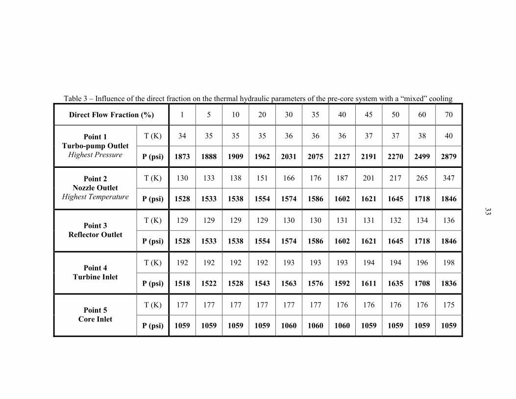
Table 3 – Influence of the direct fraction on the thermal hydraulic parameters of the pre-core system with a “mixed” cooling
33
Direct Flow Fraction (%) 1 5 10 20 30 35 40 45 50 60 70
T (K) 34 35 35 35 36 36 36 37 37 38 40Point 1 Turbo-pump Outlet
Highest Pressure P (psi) 1873 1888 1909 1962 2031 2075 2127 2191 2270 2499 2879
T (K) 130 133 138 151 166 176 187 201 217 265 347Point 2 Nozzle Outlet
Highest Temperature P (psi) 1528 1533 1538 1554 1574 1586 1602 1621 1645 1718 1846
T (K) 129 129 129 129 130 130 131 131 132 134 136Point 3
Reflector Outlet P (psi) 1528 1533 1538 1554 1574 1586 1602 1621 1645 1718 1846
T (K) 192 192 192 192 193 193 193 194 194 196 198Point 4
Turbine Inlet P (psi) 1518 1522 1528 1543 1563 1576 1592 1611 1635 1708 1836
T (K) 177 177 177 177 177 177 176 176 176 176 175Point 5
Core Inlet P (psi) 1059 1059 1059 1059 1060 1060 1060 1059 1059 1059 1059

34
Table 4 – Comparison of the highest pressure between the “parallel” and the “serial” systems
Wafer Thickness (mm) 1 1.25 1.5 1.75 2 2.25 2.5
Parallel Highest Pressure (psi) 2092 2052 2027 2010 1997 1988 1981
Serial Highest Pressure (psi) 1575 1537 1512 1495 1483 1474 1467
Table 5 – Comparison between a “full-topping” and a “bleed” cycle
Bleed Percentage 0 % Full-
Topping 5% 10% 15% 20% 25% 30%
Mass Flow Rate (kg/s) 13.86 14.55 15.25 15.94 16.63 17.33 18.02
Highest Pressure (psi) 1844 1848 1853 1859 1865 1870 1874
Highest Temperature (K) 191 185 179 174 169 164 160

CHAPTER 4 CORE HEAT TRANSFER ANALYSIS WITH FLUENT
The heat transfer in the core is a critical part of the design of the nuclear rocket
engine. The NERVA program had major problems with the core heat transfer; many
small pieces of the core were ejected from the core mainly because of the high thermal
and mechanical stress. The core of the nuclear rocket engine design of INSPI is at a very
high temperature (3000 K) and undergoes a very high pressure (1000 psi). The coolant is
heated up to high temperatures and accelerated in the channels of the core. The coolant is
a gaseous hydrogen, which allows high heat transfer with the core. The coolant flows
through the square-lattice honeycomb core at a high flow rate (several kg/s). These
specific conditions make the heat transfer model in the core different from usual core
design. This specific issue is analyzed and discussed, in this chapter and the following
one. This chapter presents the set up of the analysis.
Description of the Problem
In the first part of the thesis the calculations were performed with a nuclear rocket
engine simulation code. This program treats the heat transfer in the whole core. This heat
transfer analysis is macroscopic and uses thermal hydraulic correlations to calculate the
heat transfer in the channels. This program gives the main thermal hydraulic parameters
in the core. The unusual square geometry of the channel simplifies its fabrication. The
simulation code models the heat transfer in the square channels by considering cylindrical
35

36
channels with an equivalent diameter. In this case, the equivalent hydraulic diameter Dh,
is simply equal to the side of the square channel.
sideside
sideperimeterWetted
areaFlowDh �
�
����
44
__4
2
This formula is used to calculate the dimension of the equivalent cylindrical
channel in order to use the thermal hydraulic correlations developed for cylindrical
geometries. However considering the high temperatures and high pressures in the core,
and the dimensions of the channels, an analysis is needed to validate this approximation
for these conditions.
Equivalent channel (diameter=side of the
square channel)
Actual core channel
Figure 15 – Comparison of the heat transfer to a fluid flowing through a cylindrical or a square micro channel
The work presented in this chapter and the following one, analyses the
approximation of a square micro channel as a cylindrical micro channel, considering the
heat exchange in the channel (Figure 15). The comparison between the two types of
channel is done using FLUENT a computational fluid dynamic (CFD) code. This code
calculates the main thermal hydraulic parameters of a system considering the flow
characteristics as well as the heat transfer. By comparing the results given by FLUENT
37
for the two types of channel, the approximation is evaluated, to conclude on the use of a
cylindrical model in the specific case of the nuclear rocket engine core.
The geometry of the problem is simple. FLUENT 4.5, which includes an
integrated mesh generator, was used to perform the calculations on the two types of
channels. For further calculations, FLUENT 6 with the mesh generator GAMBIT might
give better accuracy of the results thanks a better definition of the regions near the walls.
However FLUENT 4.5 gives good results for these simple geometries.
First an overview of the CFD code FLUENT 4.5 is presented to understand the
choice of the parameters. These parameters are taken to fit with the actual conditions of
the square channels in the core.
About Fluent
As a CFD code, FLUENT solves the fundamental conservation equations for
microscopic regions. It solves the Navier-Stokes equations using a finite element method
on a grid, which is generated directly integrated in FLUENT 4.5. FLUENT 4.5 allows
building simple grids. Boundary conditions have a critical importance in the model of a
system and it will be discussed that the major problem in achieving heat transfer
evaluation is to setup an adequate model. The boundary conditions available in FLUENT,
and those chosen in the model will be also detailed in this chapter.
General Overview
Solving the Navier-Stokes equations is a real challenge, as they do not have an
exact analytical solution. Thus, numerical tools are necessary to solve numerically the
conservation equations. FLUENT is a Computational Fluid Dynamics (CFD) code, which
solves Navier Stokes equations using finite differences methods. Numerical methods are

38
numerous to solve partial differential equations (PDE), and the one used in FLUENT is
described in this chapter. Although discretization of PDE’s is powerful, it has important
limitations concerning stability of the solution and also from the size of the grid that is
chosen. The larger the grid is (or the finer the mesh size is), the more time is needed to
solve the problem. Also, the CPU time needed is generally in the order of N2 for an NxN
grid. So, the definition of the grid is a major step in the modeling of the studied system.
CFD methods, as they calculate the flow patterns and properties at every point of
a detailed grid, are very accurate. Development of a model requires assumptions to match
as well as possible the actual conditions in the channel. Also, FLUENT is solving the
conservation equations for two or three dimension cases. A three dimensional grid was
used to model the square channel and a two dimensional for the cylindrical channel. The
symmetry of the geometries is used to minimize the mesh. In the case of the cylinder, an
half axial profile of the cylinder is consider using the axial symmetry. In the case of the
square channel, a quarter of the channel is modeled, using the two planar symmetries of
the square geometry.
Basic Physical Models
For all types of problems, as shown in the user’s guide (FLUENT, 2000),
FLUENT solves the conservation equations:
�� Conservation of mass,
�� Conservation of momentum,
�� Conservation of energy (if heat transfer)
The “energy” option in the setup of the problem is chosen to calculate
temperature distributions and heat transfer phenomenon. The conservation equations are
39
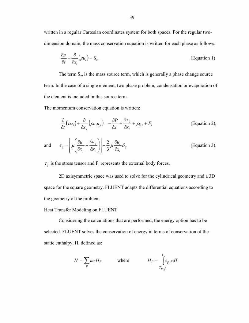
written in a regular Cartesian coordinates system for both spaces. For the regular two-
dimension domain, the mass conservation equation is written for each phase as follows:
� � mii
Suxt
��
��
�
��
� (Equation 1)
The term Sm is the mass source term, which is generally a phase change source
term. In the case of a single element, two phase problem, condensation or evaporation of
the element is included in this source term.
The momentum conservation equation is written:
� � � � iii
ij
iji
ji Fg
xxPuu
xu
t��
�
��
�
���
�
��
�
��
��� (Equation 2),
and ijl
l
i
j
j
iij x
uxu
xu
�����
��
���
�
���
�
�
��
�
�
��
�
��
32 (Equation 3).
ij� is the stress tensor and Fi represents the external body forces.
2D axisymmetric space was used to solve for the cylindrical geometry and a 3D
space for the square geometry. FLUENT adapts the differential equations according to
the geometry of the problem.
Heat Transfer Modeling on FLUENT
Considering the calculations that are performed, the energy option has to be
selected. FLUENT solves the conservation of energy in terms of conservation of the
static enthalpy, H, defined as:
��'
''i
ii HmH where ��
T
refTipi dTcH ','

40
where Tref is a reference temperature and cp,i’ is the specific heat at constant temperature
of species i'.
As the species transport equations, the energy equation solved by FLUENT
assumes that species diffusion due to pressure and external forces is negligible. Under
this assumption, the energy equation cast in terms of h can be written:
� � � � Hj
iij
ii
ijjj
iiii
iS
xu
xpu
xpJH
xxTk
xHu
xh
t�
�
��
�
��
�
��
�
����
�
����
�
�
�
�
�
��
�
�� ���
'''
(Equation 4)
where T is the temperature, � is the viscous stress tensor, Jij j’ is the flux of species j’, and
k is the mixture thermal conductivity. Sh is a source term that includes sources of
enthalpy due to the chemical reaction, radiation, and exchange of heat with the dispersed
second phase.
In conducting solid regions, FLUENT solves a simple conduction equation that
includes the heat flux due to conduction and volumetric heat sources within the solid:
'''.q
xTk
xH
t iw
iww �
�
�
�
��
�
�� (Equation 5)
where = wall density, Hw� w = wall enthalpy ( cw(T-Tref) ), kw = wall conductivity, T =
wall temperature, ' = volumetric heat source. ''.q
The previous equation is solved simultaneously with the enthalpy transport
equation, to yield a fully coupled conduction/convection heat transfer prediction. The
radiation is not considered in these experiments.

41
Turbulence Modeling on FLUENT
In this study, the flow is turbulent, as Reynolds numbers are high (about 104-106).
Reynolds number is equal to �
� hvD�Re where Dh is the hydraulic diameter, � is the
fluid density, v is the fluid velocity and µ is the fluid viscosity. As the temperature of the
gas is high, viscosity is really low, which makes the Reynolds number high. A turbulent
viscosity term has to be taken into account, as seen in the previous part. The way this
parameter is calculated depends on the turbulence model one chooses. Unfortunately,
there is no single universal model for turbulence modeling. Actually, turbulence
modeling may need to be developed for each specific case, as it depends a lot on the fluid
type and properties, and on the geometry. Turbulent flows are characterized by
fluctuating velocity fields. As these fluctuations are of very small scale or high
frequency, it is difficult and too expensive to simulate them from an engineering point of
view. Governing equations can be averaged over time or ensemble so that resulting
modified equations are much easier to solve. But then, models are needed to determine
additional unknown variables. Turbulent viscosity can be calculated with different
methods that can require more or less parameters of the flow, like turbulent kinetic
energy k, or even the dissipation rate of the turbulent kinetic energy � .
The velocity field (and any scalar quantity field) can be decomposed in two
distinct components (mean and perturbation) such as:
iii uu '��u (Equation 6)
The turbulent kinetic energy is defined as � �2,3
2,2
2,12
1 vvvk ��� , using the
perturbation terms. As the average of the perturbation term is zero and as one takes a
42
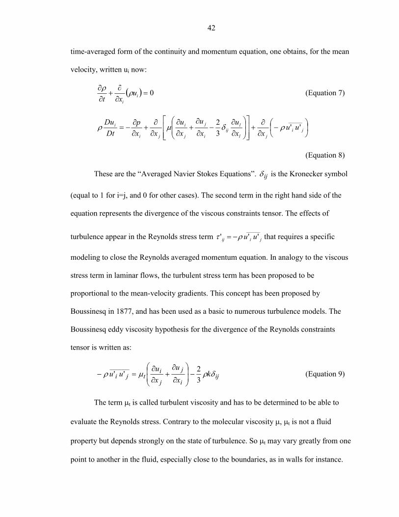
time-averaged form of the continuity and momentum equation, one obtains, for the mean
velocity, written ui now:
� � 0��
��
�
�
ii
uxt
�� (Equation 7)
��
���
��
�
�
�
�
�
�
��
�
�
��
�
�
�
��
�
�
�
�
�
�
�
���
______
''32
jijl
lij
i
j
j
i
ji
i uuxx
uxu
xu
xxp
DtDu
����
(Equation 8)
These are the “Averaged Navier Stokes Equations”. � is the Kronecker symbol
(equal to 1 for i=j, and 0 for other cases). The second term in the right hand side of the
equation represents the divergence of the viscous constraints tensor. The effects of
turbulence appear in the Reynolds stress term � that requires a specific
modeling to close the Reynolds averaged momentum equation. In analogy to the viscous
stress term in laminar flows, the turbulent stress term has been proposed to be
proportional to the mean-velocity gradients. This concept has been proposed by
Boussinesq in 1877, and has been used as a basic to numerous turbulence models. The
Boussinesq eddy viscosity hypothesis for the divergence of the Reynolds constraints
tensor is written as:
ij
' j
______
'' iij uu���
iji
j
j
itji k
xu
xu
uu ����32''
______�
��
�
�
��
�
�
�
�
�
�� (Equation 9)
The term �t is called turbulent viscosity and has to be determined to be able to
evaluate the Reynolds stress. Contrary to the molecular viscosity �, �t is not a fluid
property but depends strongly on the state of turbulence. So �t may vary greatly from one
point to another in the fluid, especially close to the boundaries, as in walls for instance.

43
Many models have been developed to calculate turbulent viscosity. Some of them are
very simple and based on empirical correlations, but other models are more complex and
mix theoretical and empirical considerations to setup transport equations for turbulence-
related quantities used to obtain the turbulent viscosity. So the Boussinesq eddy viscosity
hypothesis does not constitute the whole turbulence model, but it provides the framework
for constructing a model. The main problem is actually to determine the distribution of �t.
Seven models of turbulence can be used in FLUENT, each of them being adapted
to a certain type of situation (FLUENT, 2000):
�� Spalart-Allmaras model,
�� k- model (Standard, RNG and Realizable), �
�� Reynolds stress model and
�� Large Eddy simulation.
Two-equation models are the most widely used in engineering simulations. This
study uses the standard k-� model, which is a two-equation model and uses a Boussinesq
eddy viscosity hypothesis for the divergence of the Reynolds constraints tensor.
The k-� model is used as a better alternative to the one-equation Spalart-
Allmaras model (FLUENT, 2000). This is a very common turbulence model as it is based
on semi-empirical considerations. The standard k-� model proposed by Jones and
Launder has been the workhorse of engineering turbulence models for more than two
decades. It falls in the category of “two-equation” turbulence models based on an
isotropic eddy-viscosity concept. In this model, the transport equations of turbulent
kinetic energy (k) and its dissipation rate ( ) are solved. Basically, the transport
equations of k and � are built on the classical balance equation:
�

44
Rate of change + Convection = Diffusion + (Generation – Destruction)
The transport equations for the Standard k-� model are:
Mbkik
t
i
YGGxk
xDtDk
������
���
�
�
� �
��
� ��
�
��� (Equation 10)
where Gk is the production of turbulent kinetic energy defined as i
jjik u
uuu
�G
��� ''� ,
determined using Boussinesq assumption, Gb is the generation term due to buoyancy,
defined as it
tib x
TgG�
��
Pr�
� . YM is the dilatation dissipation term for high Mach number
flows. � is the turbulent Prandtl number for k. k
� �k
CGCGk
CxxDt
Dbk
i
t
i
2
231�
���
�
��
��
���
�
�����
���
�
�
� �
��
� (Equation 11)
where C , C and are constants, � is the turbulent Prandtl number for� . In
FLUENT, constants have the default values =1.44, =1.92, C =0.09, � =1.0
and � =1.3. These values have been determined experimentally. However, the user can
change them in FLUENT. This study used only the Standard k-� model without
changing the default constants. A detailed description of other two-equation models can
be found in the user manual.
�1
�
�2 �3C�
�1C�2C
�3 k
In this model, the turbulent viscosity is computed as �t=�C�k2/�. This value can
then be used to calculate the Reynolds stress, from the Boussinesq assumption. The main
difficulty is to choose the boundary conditions for k and� . The user guide manual
proposed the following approximations to evaluate the initial conditions for k and� .

45
�� The turbulent kinetic energy k ( can be estimated from the
turbulence intensity I defined as
)/ 22 sm
� � 8/1Re16.0 �
�HD
'�
avguuI : � �2
23 Iuk avg�
�� The turbulent dissipation rate ) can be estimated from a length
scale . Then� is approximately equal to
� /( 32 sm
hDl 07.0�
lkC
2/34/3
��� . The
constant Cµ has been determined equal to 0.09.
This research uses these methods to determine the inlet turbulence conditions, k
and � . Table 6 presents the results for the inlet turbulent parameters calculated for the
velocities considered in the experiment. It has to be noticed that these parameters are
exactly the same for both types of channel. The shape of the channel is the only factor,
which changes between the sets of calculations.
Table 6 – Turbulence parameters for the two inlet velocities
U0 (m/s) � (kg/m3) � (N.s/m2) Dh (mm) Re I k (m2/s2) � (m2/s3)
20 6 8E-06 1 1.5E04 4.81E-02 1.39 5.12
20 6 8E-06 2 3.0E04 4.41E-02 1.17 3.95
20 6 8E-06 3 4.5E04 4.19E-02 1.05 3.39
20 6 8E-06 5 7.5E04 3.93E-02 0.93 2.80
20 6 8E-06 10 15E04 3.61E-02 0.78 2.16
20 6 8E-06 20 30E04 3.31E-02 0.66 1.66
100 6 8E-06 1 7.5E4 3.93E-02 23.20 349.84
100 6 8E-06 2 15E04 3.61E-02 19.51 269.76
100 6 8E-06 3 22.5E4 3.43E-02 17.63 231.71
100 6 8E-06 5 37.5E4 3.22E-02 15.52 191.32
100 6 8E-06 10 75E05 2.95E-02 13.05 147.53
100 6 8E-06 20 150E5 2.70E-02 10.97 113.76

46
Numerical Solvers
This part will present numerical solvers available in FLUENT. Different
algorithms can be used, depending on the type of problem that needs to be solved. Also,
boundary conditions are to be chosen among the list of available models presented in this
part. All types of boundary conditions are not always compatible with each other, or even
with the type of problem, depending on the geometry or the flow conditions for example.
There are two different numerical schemes in FLUENT, the so-called
“segregated” solver and “coupled” solver. The principle of both solvers is to solve the
integral form of the equations of conservation of mass, momentum and energy over a
mesh grid. Turbulence related equations (like in the k- model) also employ these
solvers. A detailed description of both methods can be found in the FLUENT user
manual (FLUENT, 2000). This paper focuses mainly on the segregated solver.
�
Both solvers use a control volume technique. For this method, the domain is
divided in control volumes delimited by a computational grid. The grid choice depends
on the geometry, the type of problem to be solved (heat transfer, fluid flow), and the
resolution needed for the solution. One may choose simple orthogonal grid for simple
geometry where more resolution in certain regions of the domain is not needed. However,
if the focus is on boundary layers or some regions around obstacles, then one may need to
use a finer mesh grid in the interesting regions of the domain. The generation of this type
of grid may be very time consuming, and can need specific tools like GAMBIT. However
for a first evaluation, FLUENT 4.5 allows to build fine meshes for simple geometries.
The governing equations, which are actually partial differential equations, are
integrated over a control volume to obtain a set of algebraic equations involving all
47
variables. These equations are then linearized and the system obtained is solved. These
two steps (linearization and resolution) are different depending on the solver.
In the segregated solution method, starting from an initial estimation or the
current solution, the fluid properties are updated. Next, the momentum equations for
every direction are solved using current values for pressure and face mass fluxes, in order
to update the velocity field. A Poisson type equation obtained from mass conservation
and linearized momentum equation is solved to correct pressure and velocity field so that
mass conservation is satisfied. When needed, scalar quantities like energy or turbulence
are calculated (by solving appropriate equations). The last step is to check the
convergence, which is tested on the residual of the unknown parameters. The
convergence level of each residual can be chosen separately. In the segregated solution
method, terms are treated explicitly and implicitly with respect to the iteration
advancement variable. The variable treated implicitly is the equation’s dependent
variable. Thus, for each variable, we have a set of linear equations, one for each cell in
the domain. The principle of the segregated solver is that it solves a system of equations
for the variables one after the other.
Different discretization schemes are available for each governing equation. As
noted earlier, the code uses a control-volume technique. The governing equations are
integrated over the volume of the cell, such that the values of pressure and velocity are
needed at the cell faces. However, FLUENT uses a co-located scheme, meaning that both
pressure and velocity are stored at the center of the cell. Therefore, an interpolation
scheme is needed for pressure and velocity. Different schemes are available in FLUENT.
This study used the standard scheme for pressure. The momentum interpolation utilizes a

48
first order upwind scheme. It is assumed that the variable face value is equal to the cell
center value of the variable in the upstream cell. As observed, the second step, after
solving the momentum equations, is to perform a pressure and velocity field correction.
The pressure velocity coupling is realized with the SIMPLE algorithm. This algorithm
provides a pressure correction and is described in the FLUENT user’s guide (FLUENT,
2000). Since the energy equation must be solved, interpolation for energy is done using a
first order upwind scheme. This is also the case for k and � transport equations. More
extensive descriptions of numerical methods employed by FLUENT can be found in the
FLUENT user’s guide.
Definition of the Calculation
The set-up of the parameters of the experiment determines the accuracy of the
calculation. The main groups of parameters are the dimensional parameters (defined by
the grid), the material properties (defined in the entries) and the boundaries conditions
(defined both by the grid and the entries). Increasing the accuracy is always possible, but
this increase also means an increase of the computational time. The precision on the
entries has to be even. Each parameter has to be considered to increase the accuracy of
the results. The limits required for these calculations are to obtain residuals less than 10-4.
An equilibrium between the computational time and the accuracy of the parameters has to
be found to reach these limits. The parameters presented in the next section allowed
reaching the convergence of the results after about 30 minutes of iterations (8000 to 9000
iterations) for the cylindrical geometry and 3 hours (8000 to 9000 iterations) for the
square geometry.

49
Dimensional parameters
The geometry of the system is not common due to its specific dimensions. The
cooling channels in the core are long and very narrow. 500 rows of cells are considered in
length. Not to increase the computational time too much, 9 rows of cells are considered in
width (9x9 for the square channel, 9 for the cylindrical channel). The two grids designed
for the calculation are presented on the following Figure 16 and 17.
W1 W1 W1 W1 W1 W1 W1 W1 W1 W1 W1 W1 W1
W1 W2 W2 W2 W2 W2 W2 W2 W2 W2 W2 W2 W2
W1 W2 W2 W2 W2 W2 W2 W2 W2 W2 W2 W2 W2
I I I I I A A A A A A A A A A A A A
W1 W1 W1 W1 W1 W1
W2 W2 W2 W2 W2 W1
W2 W2 W2 W2 W2 W1
O O O O O
A A A A A A
(W1 = Constant temperature wall cell, W2 = Conducting wall cell, I = Inlet cell, O =
Outlet cell, A = Axis symmetry cell)
Figure 16 – Axial Profile of the mesh used for FLUENT calculations

50
S W1 W1 W1 W1 W1 W1 W1 W1
S W2 W2 W2 W2 W2 W2 W2 W1
S W2 W2 W2 W2 W2 W2 W2 W1
S W2 W2 W1
S W2 W2 W1
S W2 W2 W1
S W2 W2 W1
S W2 W2 W1
S S S S S S S S S
(W1 = Constant temperature wall cell, W2 = Conducting wall cell, I = Inlet cell, O =
Outlet cell, S = Symmetry cell)
Figure 17 – Orthogonal profile of the mesh used for FLUENT calculations
Seven types of cells are established to model the flow and the heat transfer in the
channel:
�� I: inlet cell. They model the entering flow with an inlet velocity (Ti=250 K, Vi=20 or 100 m/s)
�� O: outlet cell. They define the flow outlet
�� “Live” cell. They define the flow in the channel
�� A or S: axis or symmetry cells. They define the symmetry depending on the studied geometry
�� W1: constant temperature wall cell. They define the external contours of the channel (Tw=3000 K)
�� W2: conducting wall cell. They define the bulk of the wall of the channel. Used instead of constant temperature wall cells, they better model the heat transfer with the coolant. The characteristics of the material for these cells are the same as the actual core material: conductivity = 50 W/m.K, heat generation rate = 3000 MW/m3

51
The analysis is done on a quarter of the square channel using the symmetry on
two sides of the grid. For the cylindrical channel, only half of the cylinder is studied, one
side of the grid being a symmetry axis.
Gas Properties
The definition of the material parameters is also a key for an accurate calculation.
FLUENT allows changing the properties of the material used. The operating pressure
chosen for the calculations is 65 bars, which corresponds to the calculations performed
with the simulation code on the thermal hydraulic design of the rocket in the first part.
The properties of the fluid, which is gaseous hydrogen have been studied and listed by
INSPI. The thermal conductivity, the viscosity and the specific heat are plotted according
to the temperature on Figure 18, 19 and 20.
y = 3E-07x2 - 0.0003x + 0.3314R2 = 0.9681
0
0.5
1
1.5
2
2.5
200 700 1200 1700 2200 2700 3200
Temperature (K)
Ther
mal
con
duct
ivity
(W/m
.K)
65 bars
Poly. (65 bars)
Figure 18 – Fitting curve of the thermal conductivity of hydrogen

52
y = -1E-12x2 + 2E-08x + 4E-06R2 = 0.9989
5.0E-06
1.0E-05
1.5E-05
2.0E-05
2.5E-05
3.0E-05
3.5E-05
4.0E-05
4.5E-05
5.0E-05
200 700 1200 1700 2200 2700 3200Temperature (K)
Visc
osity
(N.s
/m2 )
65 bars
Poly. (65 bars)
Figure 19 – Fitting curve of the viscosity of hydrogen
y = 0.003x2 - 6.4781x + 17681R2 = 0.9551
10000
15000
20000
25000
30000
35000
200 700 1200 1700 2200 2700 3200
Temperature (K)
Spec
ific
Hea
t (J/
kg.m
2 )
65 bars
Poly. (65 bars)
Figure 20 – Fitting curve of the specific heat of hydrogen

53
EXCEL was used to approximate these curves with polynomial functions. The
degree of the polynomial function is limited because as explained before, increasing the
accuracy of parameters increases the computational time. The goal of this study is a
comparison between the two types of channel, not a quantitative study of one model. The
inaccuracy of the properties definition, given by the factor R2 of the fitting curve, does
not affect the comparison.
The functions used to represent the properties of H2, are:
�� Thermal conductivity: � � 7241 1031031016.3.���
�������� TTKmW�
�� Viscosity: 12286 10102104.��� ��������
���
TTsmkg
�
�� Specific heat: 32 109.2613717559.��������
���
TTKkg
JCp
at 65 bars.
Boundary Conditions
The boundary conditions determine the heat transfer from the wall. These
calculations consider the flow of gas in the channel as well as the heat transfer between
the wall and the fluid. Three cells define the wall in width. The cells of the external row
are wall cells with constant temperatures. To model the heat transfer between the wall
and the coolant, two rows of conducting wall cells are considered. The heat transfer is
modeled taking into consideration the heating from the wall to the fluid, as well as the
cooling of the wall. If only constant temperature cells were selected to model the wall,
the heat transfer between the wall and the coolant would have been poorly defined. Using
more conducting cells would have made the model more accurate, however it would have
increased the computing time. It must be noted that a conducting wall cell cannot be set

54
on the edge of the channel. Constant temperature cells replace them at the entrance and
exit faces. The conducting wall cells have to be set between other cells and that cannot be
on the edge of the grid.
To increase accuracy, a finer mesh could be generated with the software
GAMBIT to better define the region near the wall where the heat transfer takes place.
However the model used for these calculations gave satisfactory results. The wall
boundaries are defined as constant temperature (3000) K wall. The roughness of the wall
is not taken into account, considering that the material used in the core can be made very
smooth or rough according to the fabrication.
Two inlet velocities were considered: 20 and 100 m/s. These velocities
correspond to typical inlet conditions in the nuclear rocket reactor core. These two inlet
velocities correspond also to turbulent flow for most of the dimensions considered in this
study. The results of the numerous calculations are presented and discussed in the next
chapter.

CHAPTER 5 EVALUATION OF THE CYLINDRICAL APPROXIMATION FOR A SQUARE
MICROCHANNEL
This chapter shows and discusses the results of the calculations presented in the
previous chapter. First, the accuracy of the results will be discussed. Second, the
cylindrical approximation is discussed by comparing the results between the cylindrical
channel and the square channel calculations. Indeed some observations are made
considering the validity of the approximation for special conditions.
Convergence of the Calculations
FLUENT calculations are iterative. Then the validity of the results depends on the
convergence of the calculations. This convergence is characterized by the residuals of the
main parameters of the calculation.
The convergence of the calculations is required to validate the results. The model
used for these channels allowed the calculations to converge. However due to the extreme
dimensions, the thermal dynamic and hydraulic considerations and the definition of the
materials, the calculations require a large number of iterations to converge and a large
computational time. The calculations usually required at least 8000 iterations. After those
iterations, the results were checked the next 500 iterations to verify the convergence in
each case. Figure 21 presents the convergence of the velocity for one case.
55

56
0
0.10.2
0.3
0.40.5
0.60.7
0.8
0.91
1.1
1000 2000 3000 4000 5000 6000 7000 8000 9000
Number of Iterations (i)
Con
verg
ence
of t
he te
mpe
ratu
re
T(i)/
Tcon
v Calculations 1
Calculations 2
Figure 21 – Example of convergence of the results
The process of obtaining a converged solution is of great importance in FLUENT
simulations. To monitor this process, FLUENT provides a running report of the residuals
for each equation and for each iteration. The residuals are a measure of how closely each
finite difference equation is balanced, given the current state of the solution. FLUENT
computes residuals for each conservation equation by summing the imbalance in the
equation for all cells in the domain (FLUENT, 2000). The residuals of the calculation,
which represents the accuracy of the results, were less than 10-4 at the end of the
calculations for the 6 parameters: pressure, velocity (2 or 3 parameters), enthalpy,
turbulence energy and turbulence dissipation. The focus is placed on the enthalpy
residual as the calculations consider the heat transfer. This residual was kept low to
accept the convergence of the results. Figure 22 and 23 show the enthalpy residuals for
the different hydraulic diameters for the two inlet velocities (Vi=20 and 100 m/s).

57
1.E-06
1.E-05
1.E-04
1.E-03
0.75 1 2 3 5 10 20
Equivalent Hydraulic Diameter (mm)
Enth
alpy
Res
idua
lCylindrical channel
Square channel
Figure 22 – Enthalpy residual for the different calculations with Vi=20 m/s
1.E-06
1.E-05
1.E-04
1.E-03
0.75 1 2 3 5 10 20Equivalent Hydraulic Diameter (mm)
Enth
alpy
Res
idua
l
Cylindrical channel
Square channel
Figure 23 – Enthalpy residual for the different calculations with Vi=100 m/s

58
The residual is higher for bigger hydraulic diameter because of the lack of radial
definition. In fact the number of cells was kept the same for every calculations not to
interfere with the results. Then for the biggest diameter, the quality of the mesh is not as
good as for the small diameter. However even with this poor definition, the residuals are
low.
Comparison between the Square and the Cylindrical Channel
The following figures present the results of the calculations. They show the
variation of the thermal dynamic parameters after 10 cm in the channel, for the two
geometries according to the equivalent hydraulic diameter. They show the difference of
these parameters between the two types of channel for low equivalent diameters. The
calculations were done for equivalent diameters from 0.75 to 20 mm. However the
figures focus on a range between 0.75 to 5 mm.
The mass flow weighted average is calculated for each thermal hydraulic
parameter over all the cells of the surface at 10 cm after the inlet. The average mx of a
parameter x is given by the following:
�� �
�
cells
cellsm vA
xvAx
�
� )(
where x is the value of the parameter, � the density of the fluid and v its velocity for a
cell of area A.

59
Variation of the Outlet Velocity according to the Equivalent Diameter
The first two figures show the mass flow weighted average velocity after 10 cm in
the two types of channel, which is a an accurate representation of the velocity increase in
the channels. Figures 24 and 25 present the mass flux weighted average velocity variation
according to different hydraulic diameters for inlet velocities of respectively 20 and 100
m/s.
25
50
75
100
125
150
175
200
225
250
0.5 1 1.5 2 2.5 3 3.5 4 4.5 5Equivalent Hydraulic Diameter (mm)
Wei
ghte
d A
vera
ge V
eloc
ity (m
/s) Cylindrical channel
Square channel
Figure 24 – Average outlet velocity according to different hydraulic diameters (Vi=20 m/s)

60
100
200
300
400
500
600
700
800
900
0.5 1 1.5 2 2.5 3 3.5 4 4.5 5Equivalent Hydraulic Diameter (mm)
Wei
ghte
d A
vera
ge V
eloc
ity (m
/s) Cylindrical channel
Square channel
Figure 25 – Average outlet velocity according to different hydraulic diameters (Vi=100 m/s)
The figures show that the increase of velocity through the channel is much bigger
for small hydraulic diameter. It appears that the difference between the two types of
channel is very small. However for the high velocity (100 m/s) and small hydraulic
diameter (less than 3 mm), this difference seems to be significant.

61
Variation of the Outlet Temperature according to the Equivalent Diameter
The second set of figures shows the mass flow weighted average temperature after
10 cm in the two types of channels. Figures 26 and 27 present the mass flow weighted
average temperature variations according to different hydraulic diameter for inlet
velocities of respectively 20 and 100 m/s. This average only considers the flow
temperature and not the wall one. The inlet temperature of the coolant is 250 K.
The figures show that the increase in temperature through the channel is much
bigger for small hydraulic diameters. As for the velocity variations, the difference
between the two types of channel is very small. For the high inlet velocity (100 m/s) and
low hydraulic diameter (less than 3mm), this difference seems to be significant.
0
500
1000
1500
2000
2500
3000
0.5 1 1.5 2 2.5 3 3.5 4 4.5 5Equivalent Hydraulic Diameter (mm)
Wei
ghte
d A
vera
ge T
empe
ratu
re (K
)
Cylindrical channel
Square channel
Figure 26 – Average outlet temperature according to different hydraulic diameters (Vi=20 m/s)
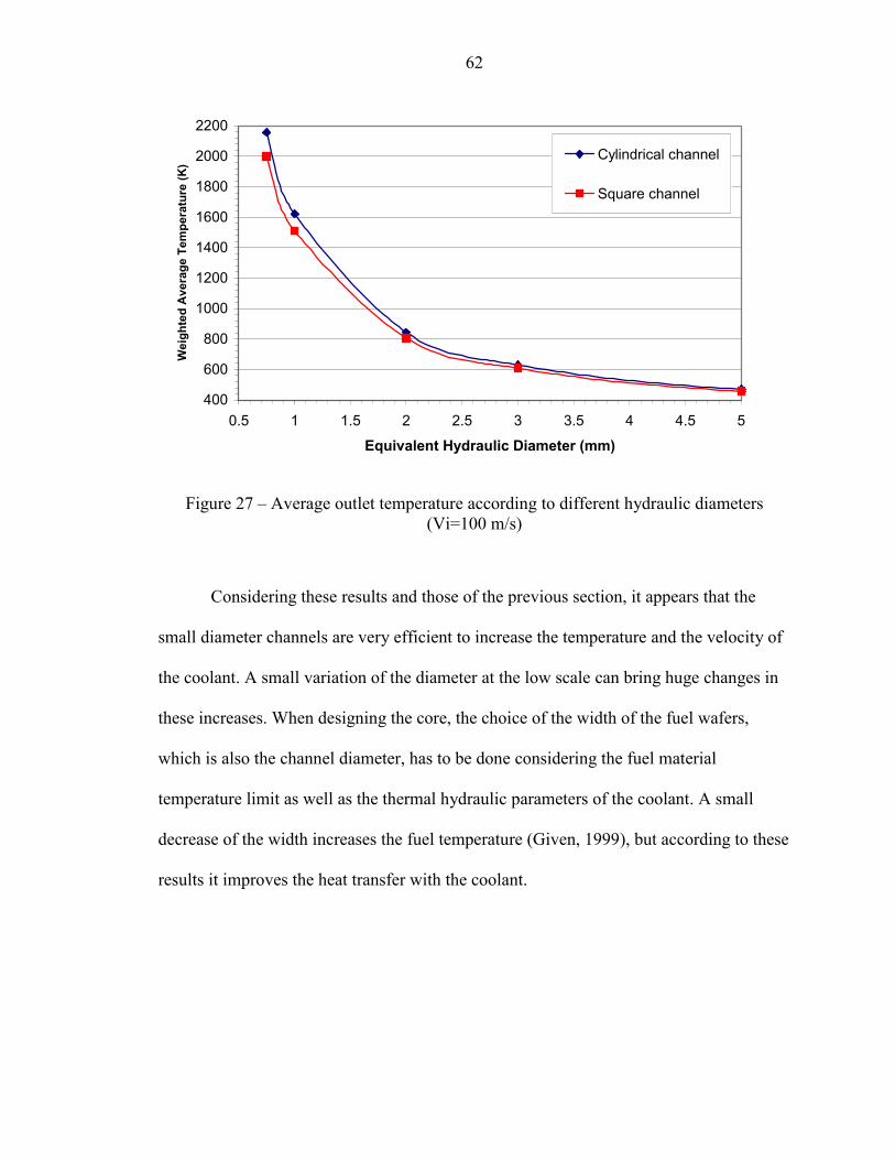
62
400
600
800
1000
1200
1400
1600
1800
2000
2200
0.5 1 1.5 2 2.5 3 3.5 4 4.5 5
Equivalent Hydraulic Diameter (mm)
Wei
ghte
d A
vera
ge T
empe
ratu
re (K
)
Cylindrical channel
Square channel
Figure 27 – Average outlet temperature according to different hydraulic diameters (Vi=100 m/s)
Considering these results and those of the previous section, it appears that the
small diameter channels are very efficient to increase the temperature and the velocity of
the coolant. A small variation of the diameter at the low scale can bring huge changes in
these increases. When designing the core, the choice of the width of the fuel wafers,
which is also the channel diameter, has to be done considering the fuel material
temperature limit as well as the thermal hydraulic parameters of the coolant. A small
decrease of the width increases the fuel temperature (Given, 1999), but according to these
results it improves the heat transfer with the coolant.

63
Variation of the Pressure Drop over 10 cm according to the Equivalent Diameter
The third set of figures shows the mass flow weighted average pressure drop per
meter over 10 cm in the two types of channels. The pressure drop is averaged as the
temperature and the velocity of the coolant even if it does not greatly vary in a section of
the flow. Figures 28 and 29 present these pressure drops according to different hydraulic
diameters for inlet velocities of respectively 20 and 100 m/s. The pressure drops have
been averaged over 10 cm, to obtain a pressure drop per unit length, which is a more
common parameter.
The plots show that the pressure drop drastically increases for small hydraulic
diameters. As in the previous sections, the difference between the two types of channel is
significant only for small hydraulic diameters (less than 3 mm) and high inlet velocity
(100 m/s).
0
10
20
30
40
50
60
70
80
90
100
0.5 1 1.5 2 2.5 3 3.5 4 4.5 5
Equivalent Hydraulic Diameter (mm)
Pres
sure
Dro
p (k
Pa/m
)
Cylindrical channel
Square channel
Figure 28 – Pressure drop according to different hydraulic diameters (Vi=20 m/s)
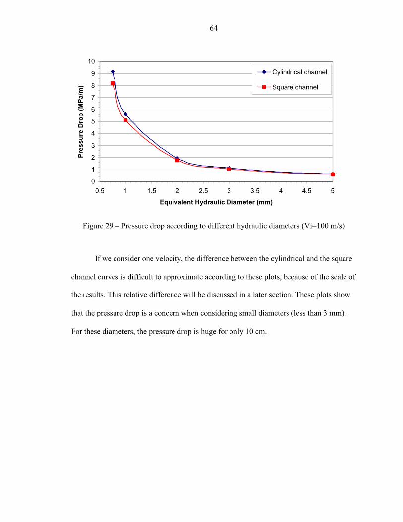
64
0
1
2
3
4
5
6
7
8
9
10
0.5 1 1.5 2 2.5 3 3.5 4 4.5 5
Equivalent Hydraulic Diameter (mm)
Pres
sure
Dro
p (M
Pa/m
)Cylindrical channel
Square channel
Figure 29 – Pressure drop according to different hydraulic diameters (Vi=100 m/s)
If we consider one velocity, the difference between the cylindrical and the square
channel curves is difficult to approximate according to these plots, because of the scale of
the results. This relative difference will be discussed in a later section. These plots show
that the pressure drop is a concern when considering small diameters (less than 3 mm).
For these diameters, the pressure drop is huge for only 10 cm.

65
Variation of the Outlet Density according to the Equivalent Diameter
The fourth set of figures shows the mass flow weighted average density of the
fluid after 10 cm in the two types of channels. Figures 30 and 31 present the density
variations according to different hydraulic diameters for inlet velocities of respectively 20
and 100 m/s.
The variations of the density follow the variations of the temperature because the
density is directly related to the temperature by the approximation presented in the
previous chapter. It has to be noticed that the inlet density is 6 kg/m3. The resulting
density after the heating in the channel is the key parameter for the exhaustion in the
nozzle of the rocket engine. The decrease in density is higher for small diameters.
0.0
0.5
1.0
1.5
2.0
2.5
3.0
3.5
4.0
0.5 1 1.5 2 2.5 3 3.5 4 4.5 5Equivalent Hydraulic Diameter (mm)
Wei
ghte
d A
vera
ge D
ensi
ty (k
g/m
3 )
Cylindrical channel
Square channel
Figure 30 – Outlet density according to different hydraulic diameters (Vi=20 m/s)

66
0.5
1.0
1.5
2.0
2.5
3.0
3.5
4.0
4.5
0.5 1 1.5 2 2.5 3 3.5 4 4.5 5Equivalent Hydraulic Diameter (mm)
Wei
ghte
d A
vera
ge D
ensi
ty (k
g/m
3 )
Cylindrical channel
Square channel
Figure 31 – Outlet density according to different hydraulic diameters (Vi=100 m/s)
The difference observed between the curves for the two types of channels
correspond to the temperature difference. The difference is enhanced for bigger diameters
because of the scale effect. The parameter to consider for the approximation is the
relative difference instead of the absolute difference. This parameter is presented in the
next section.

67
Variation of the Temperature Difference between the Two Channel Types along the Channel
A new parameter is calculated to evaluate the approximation of square channels to
cylindrical channels. The relative difference presented in this section is given by:
� � � �valuechannellcylindrica
valuechannelsquarevaluechannellcylindricadifferencerelative__
_____ �
�
This parameter is a better representation of the difference; the amplitude of the
values does not influence its result. The results presented in the previous figures are used
to calculate the relative difference. Figures 32 and 33 present the variation of the relative
differences between the two types of channel according to different hydraulic diameters
for the two inlet velocities (20 and 100 m/s).
-10%
-8%
-6%
-4%
-2%
0%
2%
4%
6%
8%
0 1 2 3 4 5 6 7 8 9 10 11 12 13 14 15 16 17 18 19 20
Equivalent Hydraulic Diameter (mm)
Rel
ativ
e D
iffer
ence
Pressure Drop
Velocity
Temperature
Density
Figure 32 – Comparison of the thermal hydraulic parameters between the two types of channels (Vi=20 m/s)

68
-12%
-10%
-8%
-6%
-4%
-2%
0%
2%
4%
6%
8%
10%
12%
0 1 2 3 4 5 6 7 8 9 10 11 12 13 14 15 16 17 18 19 20
Equivalent Hydraulic Diameter (mm)
Rel
ativ
e D
iffer
ence
Pressure DropVelocityTemperatureDensity
Figure 33 – Comparison of the thermal hydraulic parameters between the two types of channels (Vi=100 m/s)
From these two curves, we can outline some aspects of the results:
�� Generally the difference between the two models increases as the hydraulic diameter decreases. The difference is only significant for very small hydraulic diameters less than 3 mm
�� The difference in pressure drop is not negligible even for increasing hydraulic diameters
�� For the inlet velocity of 20 m/s, a sudden decrease appears for a hydraulic diameter of 0.75 mm. The flow is not highly turbulent. Table 7 presents the Reynolds number calculated at the exit. The Reynolds number for this case is about 2000. For other cases the flow is highly turbulent with high Reynolds numbers.

69
Table 7 – Reynolds number at the outlet (10 cm) for the two inlet velocities
Dh (mm) 0.75 1 2 3 5 10 20
Re (Vi=20 m/s) 2301 3502 13,438 27,507 55,926 126,696 267,444
Re (Vi=100 m/s) 14,601 25,038 85,473 159,391 304,312 656,789 1,418,073
From these observations, we can discuss the validity of the approximation of
square channels as cylindrical channels with the same hydraulic diameter:
�� The approximation is very good for macroscopic hydraulic diameters, higher than 10 mm. However for pressure drop calculations, a different hydraulic diameter should be considered. The equivalent cylindrical channel diameter should be a little bit bigger than the hydraulic diameter to correct the approximation.
�� For microscopic hydraulic diameter (less than 3 mm) and high turbulent flow, the error brought by the approximation is about 4 to 10 % for the thermal hydraulic parameters. Also for these cases, a diameter slightly higher than the equivalent hydraulic diameter should be considered.
To try to understand the difference between the results for the two types of
channels, the heat transfer is discussed in the next section. FLUENT includes a generator
of contours for most thermal hydraulic parameters. Some observations are made
concerning the variations of the heat transfer and the flow contours for the two types of
channel.

70
Observation on the Heat Transfer in the Channels
From the calculations performed on FLUENT, different profiles and contours can
be plotted. Figures 34 and 35 present the velocity contours for square channels of
different hydraulic diameter: 1 mm and 10 mm. The definition of these contours is related
to the definition of the grid for the calculations. It appears that for the small diameter
channel, the gradient of velocity in the corner of the square channel is relatively lower
than for the big diameter channel. The coolant flow in the corner of the channel is less
important. Because of this low flow in the corner, we may think that the heat transfer
between the wall and the coolant is not as good as for big diameter channels. When
comparing the results from the two inlet velocities (20 and 100 m/s), we saw that for
higher velocities the heat transfer is higher.
Figure 34 – Velocity orthogonal distribution of the 1 mm square channel after 10 cm
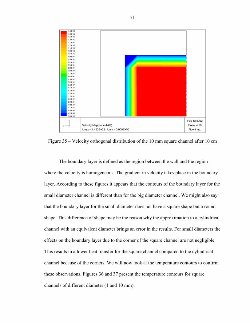
71
Figure 35 – Velocity orthogonal distribution of the 10 mm square channel after 10 cm
The boundary layer is defined as the region between the wall and the region
where the velocity is homogeneous. The gradient in velocity takes place in the boundary
layer. According to these figures it appears that the contours of the boundary layer for the
small diameter channel is different than for the big diameter channel. We might also say
that the boundary layer for the small diameter does not have a square shape but a round
shape. This difference of shape may be the reason why the approximation to a cylindrical
channel with an equivalent diameter brings an error in the results. For small diameters the
effects on the boundary layer due to the corner of the square channel are not negligible.
This results in a lower heat transfer for the square channel compared to the cylindrical
channel because of the corners. We will now look at the temperature contours to confirm
these observations. Figures 36 and 37 present the temperature contours for square
channels of different diameter (1 and 10 mm).

72
Figure 36 – Temperature orthogonal distribution of the 1 mm square channel after 10 cm
Figure 37 – Temperature orthogonal distribution of the 10 mm square channel after 10 cm
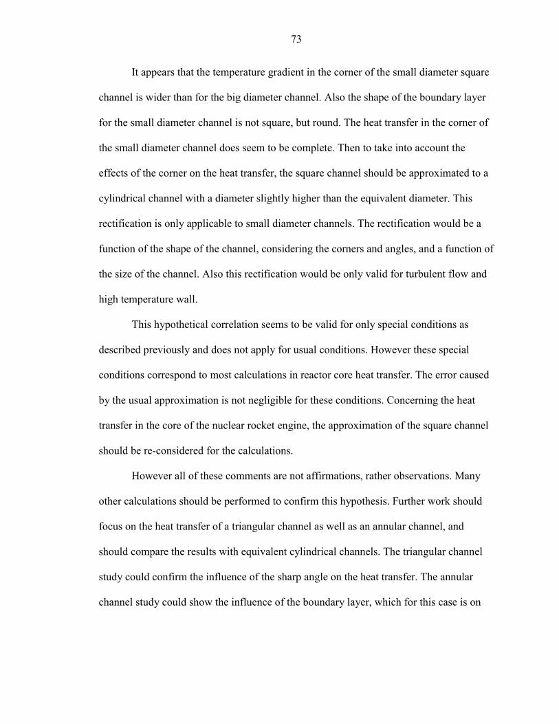
73
It appears that the temperature gradient in the corner of the small diameter square
channel is wider than for the big diameter channel. Also the shape of the boundary layer
for the small diameter channel is not square, but round. The heat transfer in the corner of
the small diameter channel does seem to be complete. Then to take into account the
effects of the corner on the heat transfer, the square channel should be approximated to a
cylindrical channel with a diameter slightly higher than the equivalent diameter. This
rectification is only applicable to small diameter channels. The rectification would be a
function of the shape of the channel, considering the corners and angles, and a function of
the size of the channel. Also this rectification would be only valid for turbulent flow and
high temperature wall.
This hypothetical correlation seems to be valid for only special conditions as
described previously and does not apply for usual conditions. However these special
conditions correspond to most calculations in reactor core heat transfer. The error caused
by the usual approximation is not negligible for these conditions. Concerning the heat
transfer in the core of the nuclear rocket engine, the approximation of the square channel
should be re-considered for the calculations.
However all of these comments are not affirmations, rather observations. Many
other calculations should be performed to confirm this hypothesis. Further work should
focus on the heat transfer of a triangular channel as well as an annular channel, and
should compare the results with equivalent cylindrical channels. The triangular channel
study could confirm the influence of the sharp angle on the heat transfer. The annular
channel study could show the influence of the boundary layer, which for this case is on

74
two surfaces of the channel. These analyses should be performed on FLUENT 6 and use
a finer mesh near the walls to consider more accurately the boundary layer.

CHAPTER 6 SUMMARY AND CONCLUSIONS
The thermal hydraulic analysis plays a major role in designing a rocket engine.
Even if the research for new rocket engines has concentrated for the past decades on the
materials and the energy production, the adaptation of the thermal hydraulic system is
necessary. The increase of the power and the operating conditions show new issues for
the thermal hydraulic systems. Nuclear power is the primary energy source of future
space rockets. In the study of nuclear rocket engines, most of the work has focused on
energy production and material evolution. However, a thermal hydraulic system must
follow similar evolutions. Research must still be conducted to reach the ultimate goal of
launching a nuclear rocket engine to Mars.
This work focuses on the thermal hydraulic system of nuclear rocket engines. The
first part deals with the improvement of the pre-core system of the nuclear rocket engine.
The second part emphasizes a specific issue concerning the heat transfer in the new core
design. This work aims to result in a better understanding of the thermal hydraulic system
for nuclear rocket engines and bring about further improvements.
The calculations in the first part use a code created at INSPI, calculating the
operating parameters of the whole system of a nuclear rocket engine. Some calculations
were already done in previous work, focusing on the improvement of the core design. In
this work, the calculations deal with the main variables of the pre-core system in order to
optimize it. By varying the organization of the system, different cooling designs are
analyzed: “serial” cooling (similar to NERVA), “parallel” cooling (similar to INSPI
75

76
rocket) and “mixed” cooling. Furthermore other variables are varied to find an optimized
system where the thermal and mechanical stresses are minimized. For each calculation
the thermal hydraulic parameters are checked at different points of the system. The main
conclusions after analysis of the different designs are:
�� The optimized system is a “serial” cooling system with a turbine by-pass ratio of about 10% with a full-topping cycle
�� If a “parallel” cooling system is considered then the reflector flow fraction which characterizes this cooling, should be taken in a range of 30 to 40%
�� A “mixed” cooling system is not efficient and for a bleed cycle the bleed percentage has to be reduced at its minimum.
This work also shows the flexibility of the simulation code and its convenience
for this kind of analysis.
The second part of this work focuses on a specific issue relative to the heat
transfer in the core of the rocket engine. The simulation code used in the first part uses a
common approximation for the heat transfer in square channels. To model this,
cylindrical channels with the same hydraulic diameter are used. FLUENT, a CFD code, is
used to compare the two channel models for different diameters and velocities, in the
conditions of the rocket engine core. According to the calculations it appears that the
model is not accurate for small diameters under 3 mm and for turbulent flows. Under
these conditions the heat transfer in the corners of the square channel seem to be the
cause of this difference. For these small dimensions and extreme conditions of
temperature, the diameter of the cylindrical channel should be taken slightly higher than
the equivalent hydraulic diameter. However these results require confirmations to be
validated. Further work should analyze the model for triangular and annular channels,

77
and do more calculations for different velocities. Also the definition of the calculations
should be improved by using a finer grid and the new version of FLUENT6.

LIST OF REFERENCES
S. ANGHAIE, G. CHEN, “A Computational Fluid Dynamics and Heat Transfer Model for Gaseous Core and Very High Temperature Gas-Cooled Reactors,” Nuclear Science and Engineering, Volume 130, 361-373 (1998) S. ANGHAIE, J.A. GIVEN, “A Computational Model for Thermal Fluid Design Analysis of Nuclear Thermal Rockets,” Nuclear Technology, Volume 117, 87-108 (January 1997) S. ANGHAIE, T. KNIGHT, R. GOUW, E. FURNAM, “ Square Lattice Honeycomb Tri-Carbide Fuels for 50 to 250 KN Variable Thrust NTP Design,” in Proceedings of NASA JPL/MSFC/UAH 12th Annual Advanced Space Propulsion, Huntsville, AL, 88-100 (Apr. 3-5 2001) G.L. BENNET, “The Past as Prologue: A Look at Historical Flight Qualifications for Space Nuclear Systems,” in Aerospace Power Proceedings of the Intersociety Energy Conversion Engineering Conference, Volume 1, 319-324, IEEE Service Center, Piscataway, NJ (1992) G. BLEEKER, J. MOODY, M. KESAREE, “The Space Nuclear Thermal Propulsion Program: Propulsion for the Twenty First Century,” in Proceedings of the Intersociety Energy Conversion Engineering Conference, Volume 1, 587-592, Warrendale, PA (1993) J.L. FINSETH, “Major Accomplishments of America’s Nuclear Rocket Program (ROVER),” in Proceedings of the Intersociety Energy Conversion Engineering Conference, Volume 1, 456-461, IEEE Service Center, Piscataway, NJ (1992) FLUENT Inc., FLUENT 4.5 User’s Guide, Fluent Inc., Lebanon, NH (October 2000) E. FURNAM, “Thermal Hydraulic Design Analysis of Ternary Carbide Fueled Square-Lattice Honeycomb Nuclear Rocket Engine,” Master’s Thesis, University of Florida (1999) E. FURNAM, S. ANGHAIE, “Thermal Hydraulic Design Analysis of Ternary Carbide Fueled Square-Lattice Honeycomb Nuclear Rocket Engine,” in Proceedings of 16th Symposium on Space Nuclear Power and Propulsion, Albuquerque, NM, Jan. 31-Feb. 4, 1999, 25-35, American Institute of Physics, NY (1999) J.A. GIVEN, “Engine System Simulation and Core Thermo-Fluid Dynamics of Nuclear Thermal Propulsion Rockets,” Master’s Thesis, University of Florida (1993)
78
79
R. GOUW, “Nuclear Design Analysis of Square-Lattice Honeycomb Space Nuclear Rocket Engine,” Master’s Thesis, University of Florida (1999) L.M. JIJI, Heat Transfer Essentials, Begell House Inc., New York (1998) R. SALKELD, D.W. PATTERSON, J. GREY, Space Transportation Systems: 1980-2000, American Institute of Aeronautics and Astronautics, New York (1978) I.H. SHAMES, Mechanics of Fluids, Third Edition, McGraw-Hill Inc., New York (1992) T.-H. SHIH, W. W. LIOU, A. SHABBIR and J. ZHU, "A New k-epsilon Eddy Viscosity Model for High Reynolds Number Turbulent Flows – Model Development and Validation," Computer Fluids 24, Volume 3, 155-180, (1995)

BIOGRAPHICAL SKETCH
Johann Plancher was born on November 29, 1977, in Avignon, France. He
graduated from Joffre High School in France. He entered the National School for Physics
in Grenoble in the fall of 1998. As part of an academic exchange, he entered the
University of Florida in the fall of 2000 as a graduate student, and obtained his French
engineer diploma in Summer 2001. Since then, he has been pursuing a Master of Science
degree in nuclear engineering sciences while working at INSPI as a graduate research
assistant.
80