Karl-Franzens-Universität Graz

Bachelor Thesis

The Aharonov-Bohm-Effect

Author:Oliver Orasch

Supervisor:Ao. Univ. Prof. Dr.

Ulrich Hohenester

December 16, 2014

ContentsPreface . . . . . . . . . . . . . . . . . . . . . . . . . . . . . . . . . . . 2Symbols and units . . . . . . . . . . . . . . . . . . . . . . . . . . . . . 3

1 AB-Effect: Theory 41.1 Introduction . . . . . . . . . . . . . . . . . . . . . . . . . . . . . . 41.2 Hamiltonian for e.m. problems . . . . . . . . . . . . . . . . . . . 51.3 Gauge Transformations . . . . . . . . . . . . . . . . . . . . . . . 6

1.3.1 General aspects . . . . . . . . . . . . . . . . . . . . . . . . 61.3.2 Schrödinger equation . . . . . . . . . . . . . . . . . . . . . 71.3.3 Phase shift in a field-free-region . . . . . . . . . . . . . . . 91.3.4 Coulomb gauge . . . . . . . . . . . . . . . . . . . . . . . . 11

1.4 Bound state problem . . . . . . . . . . . . . . . . . . . . . . . . . 121.5 Interference Experiments with e.m. potentials . . . . . . . . . . . 14

1.5.1 Double slit . . . . . . . . . . . . . . . . . . . . . . . . . . 141.5.2 Aharonov-Bohm-set-up . . . . . . . . . . . . . . . . . . . 16

1.6 Scattering AB-effect . . . . . . . . . . . . . . . . . . . . . . . . . 171.6.1 Integer α . . . . . . . . . . . . . . . . . . . . . . . . . . . 181.6.2 Half-integer α . . . . . . . . . . . . . . . . . . . . . . . . . 19

1.7 Single-valuedness of Ψ . . . . . . . . . . . . . . . . . . . . . . . . 20

2 AB-Effect: Experiments 212.1 Chambers . . . . . . . . . . . . . . . . . . . . . . . . . . . . . . . 212.2 Möllenstedt and Bayh . . . . . . . . . . . . . . . . . . . . . . . . 222.3 Tonomura et al. I . . . . . . . . . . . . . . . . . . . . . . . . . . . 232.4 Tonomura et al. II . . . . . . . . . . . . . . . . . . . . . . . . . . 24

3 Quantum Interference devices 263.1 AB-Effect in ring structures . . . . . . . . . . . . . . . . . . . . . 26

PrefaceThis thesis sums up the theoretical prediction and the experimental confirma-tion of the so-called Aharonov-Bohm-Effect [AB-Effect]. With their work YakirAharonov and David Bohm revolutionized the role of electromagnetic poten-tials in physics. To show that, simple demonstrative examples, groundbreakingexperiments, as well as applications will be presented.

The thesis is divided in three major chapters. We start with a section, whichdescribes the required theory to understand the processes associated with theAB-effect. It covers the gauge transformation, the basic quantum mechanicsand further examples, which point out the consequences of electromagnetic po-tentials. Concluding this chapter, the main work of Aharonov and Bohm willbe presented.

The second chapter concentrates on the experimental confirmation of the AB-effect, respectively on the attempts to show the influence of electromagneticpotentials. Starting with the early experiments of Chambers and Möllenstedtand Bayh, using mainly electron biprisms, we end up at Tonomura’s set-ups,where "electron- and optical-holographic techniques [were] employed". [5]

Concluding this thesis the last chapter deals with one application of the AB-effect. The consequences of miniaturization - in reference to the AB-effect - willbe shown.

Oliver Orasch Graz, December 16, 2014

2

Symbols and unitsCommon symbols used during the thesis:

~A(~x, t) ... vector potential on location ~x

~B(~x, t) ... magnetic field on location ~x

φ(~x, t) ... electrostatic potential on location ~x

~E(~x, t) ... magnetic field on location ~x

∆ϕ ... relative phase shift/ phase difference

φ ... magnetic flux through a surface σ

H0 ... Hamiltonian in a region without electromagnetic potentials or fields

H ... general Hamiltonian

e0 ... unit charge

e = −e0 ... charge of an electron

c ... velocity of light

~ ... reduced Planck constant

i ... imaginary unit

ψ0(~x, t) ... wave function for regions without electromagnetic potentials or fields

ψ(~x, t) ... general wave function

Ψ ... composit wave function

Λ(~x, t) ... arbitrary gauge function

Due to the appearance of electrodynamics, the Gaussian unit system will beused. That means

[φ(~x, t)] =[~A(~x, t)

]and

[~B(~x, t)

]=[~E(~x, t)

],

where "[...]" denotes the unit of a physical quantity. [12]

3

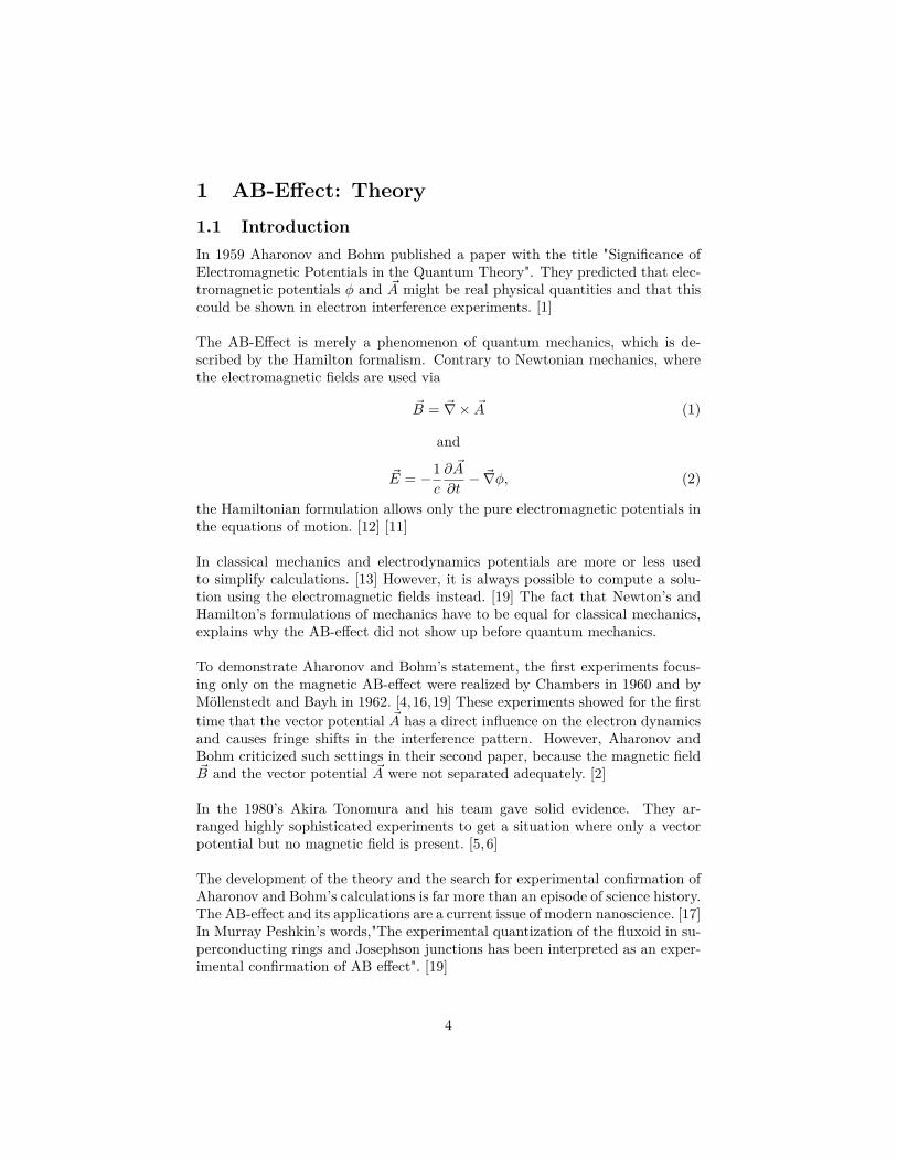
1 AB-Effect: Theory1.1 IntroductionIn 1959 Aharonov and Bohm published a paper with the title "Significance ofElectromagnetic Potentials in the Quantum Theory". They predicted that elec-tromagnetic potentials φ and ~A might be real physical quantities and that thiscould be shown in electron interference experiments. [1]

The AB-Effect is merely a phenomenon of quantum mechanics, which is de-scribed by the Hamilton formalism. Contrary to Newtonian mechanics, wherethe electromagnetic fields are used via

~B = ~∇× ~A (1)

and

~E = −1c

∂ ~A

∂t− ~∇φ, (2)

the Hamiltonian formulation allows only the pure electromagnetic potentials inthe equations of motion. [12] [11]

In classical mechanics and electrodynamics potentials are more or less usedto simplify calculations. [13] However, it is always possible to compute a solu-tion using the electromagnetic fields instead. [19] The fact that Newton’s andHamilton’s formulations of mechanics have to be equal for classical mechanics,explains why the AB-effect did not show up before quantum mechanics.

To demonstrate Aharonov and Bohm’s statement, the first experiments focus-ing only on the magnetic AB-effect were realized by Chambers in 1960 and byMöllenstedt and Bayh in 1962. [4,16,19] These experiments showed for the firsttime that the vector potential ~A has a direct influence on the electron dynamicsand causes fringe shifts in the interference pattern. However, Aharonov andBohm criticized such settings in their second paper, because the magnetic field~B and the vector potential ~A were not separated adequately. [2]

In the 1980’s Akira Tonomura and his team gave solid evidence. They ar-ranged highly sophisticated experiments to get a situation where only a vectorpotential but no magnetic field is present. [5, 6]

The development of the theory and the search for experimental confirmation ofAharonov and Bohm’s calculations is far more than an episode of science history.The AB-effect and its applications are a current issue of modern nanoscience. [17]In Murray Peshkin’s words,"The experimental quantization of the fluxoid in su-perconducting rings and Josephson junctions has been interpreted as an exper-imental confirmation of AB effect". [19]

4

1.2 Hamiltonian for e.m. problemsTo quote Richard Feynman, "Know your Hamiltonian!" [10], it is very revealingto analyze the workhorse of non-relativistic quantum mechanics. Therefore westart at the very beginning, at classical mechanics. The Hamilton-function inclassical mechanics is equal to the energy of the system,

H = T + V. (3)

This holds for arbitrary potentials V that are independent of the particle veloc-ity, whereas the kinetic energies T depend quadratically on it. [11] In general,the Hamiltonian-function can be written as

H = ~p 2

2m + V (~x), (4)

with the momentum ~p and the particle mass m.

To apply the classical Hamilton-function to quantum mechanics, one has toreplace the variables ~p and ~x by operators, which will be denoted by a "hat" ontop of the variable.

In general the Hamilton-operator (Hamiltonian) takes the form

H = ~p 2

2m + V (~x), with ~p = ~i~∇. (5)

Applying the Hamiltonian to electromagnetic problems, the kinematic momen-tum has to be replaced by [21]

m~x = ~p− e

c~A, (6)

where ~p is the canonical momentum and ~A the vector potential. Furthermore,the potential energy contribution has to be extended by eφ(~x), which is thepotential energy due to an electrostatic potential.With the last replacements the Hamiltonian allows to treat arbitrary problemsinvolving electromagnetic fields for a scalar particle, and transforms to [20]

H = 12m

[~p− e

c~A]2

+ eφ(~x) + V (~x), (7)

where V (~x) is an additional arbitrary contribution to the potential energy, whichwill be set to zero in the following.

Now we are able, to write down the general Schrödinger equation for purelyelectromagnetic problems.

i~∂

∂tψ(~x, t) =

[1

2m

[~p− e

c~A]2

+ eφ(~x)]ψ(~x, t) (8)

Due to the fact that we are only interested in field-free-regions, there does notenter a spin contribution.

5

1.3 Gauge TransformationsThe fact that the electromagnetic fields are constructed by differential operatorsshows that the electromagnetic potential Aµ =

(φ, ~A

)is well defined up to the

derivative of an arbitrary function ∂µΛ. This property is called gauge freedomand has to be fixed, as we will see later. Due to the gauge properties of φ and~A, they are often called gauge fields. [9] These points will be described in moredetail in the following.

1.3.1 General aspects

Generally, the curl of a conservative field vanishes [14],

~∇×[~∇Λ(~x, t)

]= 0. (9)

Therefore the magnetic field ~B does not change under a gauge transformationof the form

~A(~x, t) −→ ~A(~x, t) + ~∇Λ(~x, t). (10)

In this case, Λ(~x, t) is an arbitrary and real scalar field, a so-called gauge func-tion. [13]

To grant the same for the electric field

~E = −1c

∂ ~A

∂t− ~∇φ, (11)

one has to insert (10) in (11).

~E′ = −1c

∂ ~A′

∂t− ~∇φ′ = −1

c

∂

∂t

[~A+ ~∇Λ

]− ~∇φ′ != ~E (12)

It follows that~E = −1

c

∂ ~A

∂t− ~∇

[φ′ + 1

c

∂Λ∂t

](13)

and the corresponding gauge transformation reads off as

φ(~x, t) −→ φ(~x, t)− 1c

∂Λ(~x, t)∂t

. (14)

In the language of 4-vectors, the gauge transformation of the electromagneticfields becomes

Aµ −→ Aµ − ∂µΛ,

with Aµ =(φ, ~A

)and ∂µ =

(1c∂∂t ,−~∇

). [11]

6

1.3.2 Schrödinger equation

Next it is important to check what happens to the general Schrödinger equation,if a gauge transformation of the potentials is performed. Starting at

i~∂

∂tψ =

[1

2m

[p− e

c~A]2

+ eφ(~x)]ψ, (15)

we insert the transformed potentials ~A′ and φ′.

i~∂

∂tψ =

=[

12m

(p− e

c~A(~x, t)− e

c~∇Λ(~x, t)

)2+ e

(φ(~x, t)− 1

c

∂Λ(~x, t)∂t

)]ψ (16)

i~(∂

∂tψ − ie

c~ψ∂Λ(~x, t)∂t

)=

=[

12m

(p− e

c~A(~x, t)− e

c~∇Λ(~x, t)

)2+ eφ(~x, t)

]ψ (17)

A closer analysis of the l.h.s. of (17) shows that this part can also be transformedusing

ψ = ψ′e−iS(~x,t), with S(~x, t) ≡ e

~cΛ(~x, t). (18)

To show this, we take the time derivative of (18) and write explicitly

∂

∂tψ = e−iS(~x,t) ∂

∂tψ′ − ψ′ie−iS(~x,t) ∂

∂tS(~x, t) = (19)

=[e−iS(~x,t) ∂

∂t− ie−iS(~x,t) ∂

∂tS(~x, t)

]ψeiS(~x,t). (20)

Multiplying (19) to the left with eiS(~x,t), we find

eiS(~x,t) ∂

∂tψ =

[∂

∂t− i ∂

∂tS(~x, t)

]ψeiS(~x,t). (21)

By replacing the time derivatives in (21) by spatial ones, ~∇ can be transformedtoo. In general such a transformation looks like [21]

ef(x) ∂

∂x=(∂

∂x− ∂f

∂x

)ef(x). (22)

With the approach of (18) it is possible to gauge transform (15). The first step

7

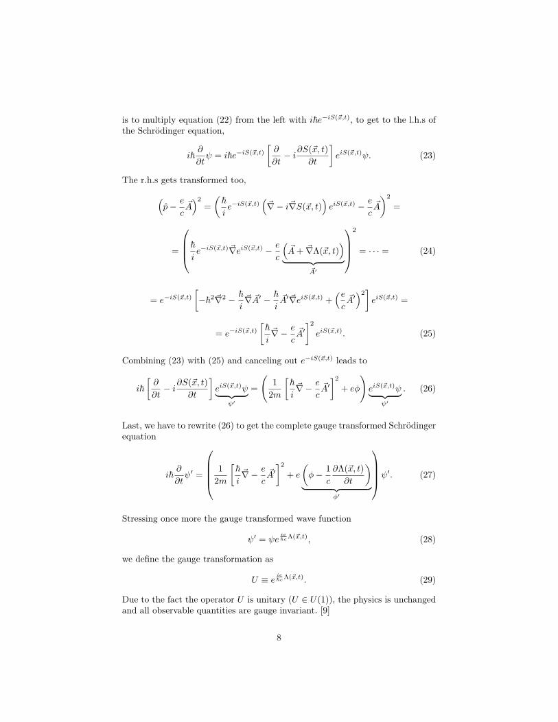
is to multiply equation (22) from the left with i~e−iS(~x,t), to get to the l.h.s ofthe Schrödinger equation,

i~∂

∂tψ = i~e−iS(~x,t)

[∂

∂t− i∂S(~x, t)

∂t

]eiS(~x,t)ψ. (23)

The r.h.s gets transformed too,(p− e

c~A)2

=(~ie−iS(~x,t)

(~∇− i~∇S(~x, t)

)eiS(~x,t) − e

c~A

)2=

=

~ie−iS(~x,t)~∇eiS(~x,t) − e

c

(~A+ ~∇Λ(~x, t)

)︸ ︷︷ ︸

~A′

2

= · · · = (24)

= e−iS(~x,t)[−~2~∇2 − ~

i~∇ ~A′ − ~

i~A′~∇eiS(~x,t) +

(ec~A′)2]eiS(~x,t) =

= e−iS(~x,t)[~i~∇− e

c~A′]2eiS(~x,t). (25)

Combining (23) with (25) and canceling out e−iS(~x,t) leads to

i~[∂

∂t− i∂S(~x, t)

∂t

]eiS(~x,t)ψ︸ ︷︷ ︸

ψ′

=(

12m

[~i~∇− e

c~A′]2

+ eφ

)eiS(~x,t)ψ︸ ︷︷ ︸

ψ′

. (26)

Last, we have to rewrite (26) to get the complete gauge transformed Schrödingerequation

i~∂

∂tψ′ =

12m

[~i~∇− e

c~A′]2

+ e

(φ− 1

c

∂Λ(~x, t)∂t

)︸ ︷︷ ︸

φ′

ψ′. (27)

Stressing once more the gauge transformed wave function

ψ′ = ψeie~cΛ(~x,t), (28)

we define the gauge transformation as

U ≡ e ie~cΛ(~x,t). (29)

Due to the fact the operator U is unitary (U ∈ U(1)), the physics is unchangedand all observable quantities are gauge invariant. [9]

8

This can easily be shown, by computing the expectation value of an arbitraryHermitian operator O [2]

〈O′〉 = 〈UOU−1〉 =∫Rψ′∗UOU−1ψ′dx =

=∫Rψ∗ U−1U︸ ︷︷ ︸

1

OU−1U︸ ︷︷ ︸1

ψdx = 〈O〉, (30)

where O′ = UOU−1 is the gauge transformed O.Furthermore, we use the last argument to relate the Hamiltonian H0, whichholds at a time where the magnetic flux is zero, to a time where the vectorpotential is present. [19]

i~∂

∂tψ = H0ψ ⇔ i~

∂

∂tUψ = UH0U

−1Uψ (31)

Rewriting (31) the Schrödinger equation takes the form

i~∂

∂tψ′ = Hψ′ with H = UH0U

−1 (32)

Concluding this section, we have found that the phase of the gauge transforma-tion U depends on the used gauge. [20]

1.3.3 Phase shift in a field-free-region

Consider a experiment where at first no magnetic field is used. Later on aconstant magnetic flux is switched on adiabatically, but due to the chosen set-up it is enclosed to an impenetrable cylinder. Moreover, we wait long enoughtill

~A(~x, t) = ~A(~x) (33)

holds. This corresponds to a gauge transformation of the kind [8]

~A(~x) = ~A0(~x) + ~∇Λ(~x) with | ~A0| = 0. (34)

The justification of that lies in

~B = 0 = ~∇× ~A ⇔ ~A = ~∇Λ, (35)

since the wave function of the electron cannot enter the regime of the magneticfield. [21]

Henceforth the gauge function Λ(~x) takes the form

Λ(~x) =∫ ~x

~x0

~A(~x′)d~x′, (36)

9

where the integration is carried out on an arbitrary path in space. [21] If~B = ~∇ × ~A = 0, the line integral depends only on the beginning ~x0 and theending ~x, not on the path itself. [11, 13]

To give (36) meaning, we consider integrals of the form∫ ~x

~x0, 1~A(~x′)d~x and

∫ ~x

~x0, 2~A(~x′)d~x′,

with 1 and 2 denoting different paths. These paths have the same starting andending point and enclose therefore the surface σ. See Figure 3 for graphicalinterpretation. Next, one can use the magnetic flux through the specific surfaceσ,

φ =∫σ

~B · d~σ (37)

where σ is enclosed by the curve that path 1 and path 2 encircle. [21] Now weuse the relation [12]

~B = ~∇× ~A, (38)

to get to ∫σ

~B · d~σ =∫σ

[~∇× ~A

]· d~σ. (39)

Stoke’s theorem allows us to transform the surface integral to a line integralover the boundary of σ. [14]

φ =∮∂σ

~A · d~x′ =∫ ~x

~x0, 1~A · d~x′ +

∫ ~x0

~x, 2~A · d~x′ =

=∫ ~x

~x0, 1~A · d~x′ −

∫ ~x

~x0, 2~A · d~x′ (40)

In conclusion, it is important to note that path 1 and 2 encircle a shielded mag-netic flux on different sides. The wave functions emitted at point ~x0 propagateeither on path 1 or 2 and get detected on point ~x. Due to their differing phases,they will interfere. As it turns out, this depends on the magnetic flux theirpaths encircle.

To generalize the discussion of phase shifts in regions where the magnetic fieldis absent, it is important to point out that analog methods can also be usedfor the electric case. Due to the 4-vector formulation of electrodynamics the4-potential can be written as [12]

Aµ(x) = (φ(~x, t),− ~A(~x, t)), with x = t, x, y, z. (41)

The space-time line element which we need for integration looks like

dxµ = (cdt, d~x). (42)

10

With this generalization the electromagnetic flux takes the form

e

~c

∮Aµ(x)dxµ = e

~c

[∮cφ(~x, t)dt−

∮~A(~x, t)d~x

], (43)

where the integration is carried out on a closed curve in space-time. [2]

1.3.4 Coulomb gauge

Since we are interested in the pure magnetic AB-effect, we choose

φ(~x, t) = 0 (44)

and fix the gauge with the so-called Coulomb-gauge [19]

~∇ · ~A = 0. (45)

Additionally all our idealized problems show plane polar symmetry, and due tothe choice ~B ‖ ez we expect ~A ‖ eθ. Therefore, the following integration can becarried out [1]

φ =∮

~A(~x)d~x =∫ 2π

0Aθρdθ = 2πρAθ. (46)

It follows that~A(θ, ρ) = φ

2πρ eθ. (47)

This choice as well satisfies the Coulomb-condition

~∇ · ~A = 1ρ

∂

∂θ

φ

2πρ = 0 (48)

and represents a suitable function for the the vector potential, since it vanishesat ρ → ∞. ~A 6= ~A(θ) exhibits once more polar symmetry.

11

1.4 Bound state problemBefore we deal with experimental set-ups and interference it is very revealing totake a look on the bound state AB-effect. This shows at least mathematicallythe influence of the vector potential ~A on an electron. Consider the set-up shown

Figure 1: Electron orbiting magnetic flux [19]

in Figure 1, where an electron encircles a solenoid on a one-dimensional wirewith radius ρ. Assuming the solenoid’s length infinite, guarantees ~B = 0 on theoutside of the cylinder. Without loss of generality we, choose ~B‖ez, so φ > 0.Due to the cylindrical symmetry we use polar coordinates with the azimutalangle θ. Here, the Schrödinger equation takes the form [13,19,21]

12m

[~i~∇− e

c~A

]2ψ(θ) = 1

2m

[−i~1

ρ

∂

∂θ− e

cAθ

]2ψ(θ) =

= ~2

2mρ2

[− ∂2

∂θ2 + i2 ec~φ

π

∂

∂θ+(e

~cφ

2π

)2]ψ(θ) = Eψ(θ). (49)

The factor of 2 at the single derivative ∂θ arises due to the commutator

[∂θ, Aθ]ψ(θ) = ∂θ (Aθψ(θ))−Aθ∂θψ(θ) = ψ(θ)∂θAθ = 0. (50)

=⇒ ∂θ (Aθψ(θ)) = Aθ∂θψ(θ) (51)

To write (49) more transparently we define φ0 ≡ πe ~c and rewrite

∂2ψ(θ)∂θ2 − i2 φ

φ0︸︷︷︸≡β

∂ψ(θ)∂θ

+

2mEρ2

~2 − φ2

φ20︸︷︷︸

≡β2

︸ ︷︷ ︸

≡ε

ψ(θ) = 0 (52)

This ordinary differential equation with constant coefficients is solved by thewave ansatz [13]

ψ(θ) = Ceiλθ, (53)

12

with λ = β ±√β2 + ε = φ

φ0± ρ

~√

2mE. (54)

To specify the parameter λ, we have to consider the continuity of the wavefunction at 2π → 0.

ψ(2π) = ψ(0) ⇒ 1 = ei2πλ (55)

From equation (55) follows that λ has to be integer, we call it l. Furthermore,ψ has to be normalized to 1 so C becomes∫ 2π

0dθ|Ceilθ|2 = 1 ⇒ C = 1√

2π(56)

Now the complete wave function is [19]

ψ(θ) = 1√2πeilθ (57)

With the computed wave function, the energy spectrum becomes

~2

2mρ2

[−i ∂∂θ− φ

φ0

]2ψ(θ) = ~2

2mρ2

[l − φ

φ0

]2ψ(θ) = Elψ(θ). (58)

El = ~2

2mρ2

[l − φ

φ0

]2= ~2

2mρ2

[l − eφ

2π~c

]2with l ∈ Z (59)

Thus, the energy spectrum of the bound states depends directly on the magneticflux, though the magnetic field is zero outside of the solenoid. Considering pos-itive l as counterclockwise and in contrary negative l as clockwise rotations, wecan interpret equation (59). If the particle orbits the solenoid counterclockwisewith a certain l, the energy would be higher (since e = −e0 < 0), in comparisonto the opposite case. [13]

The calculation above can be generalized, by allowing the electron to move in aradially symmetric potential V (ρ) around the magnetic flux, which is shieldedby a barrier or impenetrable cylinder. The main conclusion of this slightly so-phisticated problem reveals once more that the energy spectrum depends on theenclosed magnetic flux. [8]

The value of the introduced constant 2φ0 is in Gaussian units [20]

2φ0 = 2π~ce

= hc

e= 4.135× 10−7Gauss cm2 (60)

and has further physical interpretation. For reasons that will come up laterin this discussion, the introduced constant is the named "fundamental unit ofmagnetic flux".

13

1.5 Interference Experiments with e.m. potentialsTo understand the upcoming experimental set-ups, it is very important to clar-ify the general concept of interference experiments which are designed to showthe influence of electromagnetic potentials on electrons.

Interference in general occurs at the superposition of waves. That argumentholds for light waves, as well as for electron waves. Furthermore, to get station-ary fringes (interference pattern), the superposed waves have to be coherent.Two superposed waves are coherent if their time-dependent wave functions areequal except for a phase difference ∆ϕ,

ψ1(t) = const. × ψ2(ωt+ ∆ϕ). (61)

If the wave packets do not spatially overlap, there is no way that they can in-terfere. [15]

Therefore, one important feature of interference experiments is to create time-independent fringes. To achieve such interference patterns, one can either useset-ups that create stationary fringes anyway and add electromagnetic flux asperturbation, or use the pure electromagnetic potentials themselves instead.But it is very challenging to arrange such experiments, because the electrostaticpotential φ and the vector potential ~A have to be separated carefully from theelectromagnetic fields ~E and ~B.

1.5.1 Double slit

For better understanding of Aharonov and Bohm’s attempt, it is possible to il-lustrate the influence of vector potential using a double slit experiment. Figure1 shows a classical double slit experiment. The continuous line represents theoutcome of the experiment if no magnetic flux is present, while the dashed line

bElectronsource

Interferencescreen

Path 1

Path 2

Enclosed magnetic

fluxA

B

Figure 2: Double slit experiment [9]

14

suggests interaction between the vector potential and the electron.

As shown in section 1.3.3 the wave function in a region with a non-zero vectorpotential ~A is

ψ = ψ0eie~c

∫~A(~x)d~x (62)

where ψ0 represents the free case wave function. At first, to compute the inter-ference pattern, we close one of the slits and arrange the wave functions. [21]

ψ1 = ψ1,0eie~c

∫1~A(~x)d~x (63)

ψ2 = ψ2,0eie~c

∫2~A(~x)d~x (64)

The final result for both slits open arises at the superposition of (63) and (64),

Ψ = ψ1 + ψ2 = ψ1,0eie~c

∫1~A(~x)d~x + ψ2,0e

ie~c

∫2~A(~x)d~x

. (65)

Next we extract the phase factor of ψ2 and this leads to

Ψ =[ψ1,0e

ie~c

[∫1~A(~x)d~x−

∫2~A(~x)d~x

]+ ψ2,0

]eie~c

∫2~A(~x)d~x

. (66)

Stressing the calculations we did in section 1.3.3, the complete wave functioncan be written as [21]

Ψ =[ψ1,0e

ie~cφ + ψ2,0

]eie~c

∫2~A(~x)d~x

. (67)

Using equation (67) we can write down the probability density P. [21]

P = |Ψ|2 = ΨΨ∗ =

=[ψ1,0e

ie~cφ + ψ2,0

]eie~c

∫2~A(~x)d~x ×

[ψ1,0e

ie~cφ + ψ2,0

]∗e− ie

~c

∫2~A(~x)d~x =

= |ψ1,0|2 + |ψ2,0|2 + 2Re(ψ∗1,0ψ2,0e

− ie~cφ)

(68)

Summing up the last calculations, it is important to note that the shift ofthe interference pattern depends numerically on the enclosed magnetic flux.This set-up should approximately show how interference pattern are shifted ifa magnetic flux is switched on. Though for computing the AB-wave functions,it is not important to add a double slit to the experiment, as we will see in thenext section. [3] Using a double slit, however, is illustrative because the wavefunctions take the form of cylindrical waves. [21]

15

1.5.2 Aharonov-Bohm-set-up

For showing the magnetic AB-effect Aharonov and Bohm suggested the follow-ing experimental setting:

Solenoid

Interferenceregion

Electronsource

Path 1

Path 2BA

Metal guard

Figure 3: Interference Experiment in the sense of Aharonov and Bohm [1]

Figure 3 is just a schematic representation of actually realized experiments, butit can be used for the calculation of the phase shift. The technical details toarrange such experimental set-ups will be discussed in section "AB-Effect: Ex-periments".

As can be seen in the figure, the electrons are emitted by a source. At pointA the beam is split coherently, to focus it later on to point B, where the inter-ference pattern can be observed. [19] On their paths (1 or 2) the electrons arefully shielded of the magnetic field. Because (i) the magnetic field of the infinitesolenoid exists only on its inside [12] and (ii) the metal guard is arranged in away no electron can enter the inside of the solenoid. The assumption that thesolenoid is infinite, can actually be realized if the magnetic flux is enclosed byan impenetrable cylinder. [20]

The fact that the magnetic field of the solenoid vanishes on the outside andis constant on the inside, shows that the vector potential ~A cannot vanish ev-erywhere. [19]

Similar to the wave function in section 1.5.1, one can arrange the general AB-wave function like this:

Ψ =[ψ1,0e

ie~cφ + ψ2,0

]eie~c

∫2~A(~x)d~x

, (69)

where ψ1,0 and ψ2,0 represent the undisturbed wave function on paths 1 and2. [3] In general, this problem is not trivial, so Aharonov and Bohm simplifiedthe calculation by setting the radius of the flux line to zero. Therefore, theAB-effect reduces to an incoming plane electron wave that gets scattered at theflux line. [1]

16

1.6 Scattering AB-effectTo obtain exact solutions for the scattering states, Aharonov and Bohm fixedthe flux, but assumed a vanishing radius. The associated stationary Schrödingerequation in cylindrical coordinates takes the form [1][

12m

[~i~∇− e

c~A

]2+ eφ(~x)

]ψ = · · · =

=[∂2

∂ρ2 + 1ρ

∂

∂ρ+ 1ρ2

(∂

∂θ+ iα

)2+ k2

]ψ = 0. (70)

Where ~k is the wave vector,

|~k| = k = 1~√

2mE, (71)

and a flux parameterα = −eφ

ch. (72)

In the limit of vanishing flux-radius, it is justified to assume the incoming wavefunction as a single plane wave [1]

ψ0 = e−i~k~x = e−ikρ cos θ. (73)

Due to the gauge transformation (29), we are able to compute the disturbedplane wave ψ,

ψ = e−ikρ cos θeie~c

∫ ~x~x0

~A(~x′)d~x′

. (74)

Combining (72) and the Coulomb-gauge condition, the integral in the phase canbe computed ∫ ~x

~x0

~A(~x′)d~x′ =∫ θ

0Aθdθ = φ

2π θ (75)

and the wave function takes the form [3]

ψ = e−ikρ cos θe−iαθ. (76)

It is obvious that (76) does not fulfill the condition ψ(ρ = 0) = 0, but, as we willsee later on, this is a special case for integer α and has to be treated separately.Furthermore, diffraction has not been considered. Aharonov and Bohm statedthat this contribution can be neglected. [1] In the end, equation (76) is a correctincoming wave function for this problem.

The next step is, to compute the exact scattering states Ψ. We expand thewave function ψ in partial waves, in eigenstates of the angular momentum op-erator. [3, 21]

17

We find that the AB-wave function is proportional to a superposition of positiveorder Bessel-functions J(kρ)|l+α|. [1]

Ψ =∞∑

l=−∞(−i)|l+α|J|l+α|(kρ)eilθ (77)

The achievement of Aharonov and Bohm was the interpretation of Ψ. Theyconverted the exact wave function to a manageable form of [21]

Ψ = e−i~k~x + e±ikρ√

rf(θ). (78)

Now one can read off the scattered wave function and the scattering amplitudef~k(θ). The general solution takes the form [1] [19]

Ψ = e−i~k~x + eikρ√

2πikrsin πα e

−i θ2

cos θ2. (79)

The scattering amplitude reads off as

f(θ) = sin πα√2πi

e−iθ2

cos θ2. (80)

With the resulting scattering amplitude, we are able to compute the differentialscattering cross section [21]

dσdΩ = |f(θ)|2 = 1

2πsin2 πα

cos2 θ2. (81)

1.6.1 Integer α

Consider nowα = n, n ∈ Z. (82)

With this assumption, sin πn = 0, ∀ n ∈ Z and (76) takes the form

Ψ = e−i~k~x. (83)

This means that there is no observable effect on the electron wave - no interfer-ence - if the flux is quantized by integral numbers. [19]

However, this actually is already revealed by the very general equation (68),where the interference pattern is determined by the phase factor e ie~cφ. Rewrit-ing the phase factor leads to vanishing interference

eie~cφ = e

2πiehc φ = e−i2πα = e−i2πn = 1. (84)

In other words: (83) is a correct wave function for this case and it is not im-portant if it vanishes at ρ = 0 or not, because there is no observable effectanyway.

18

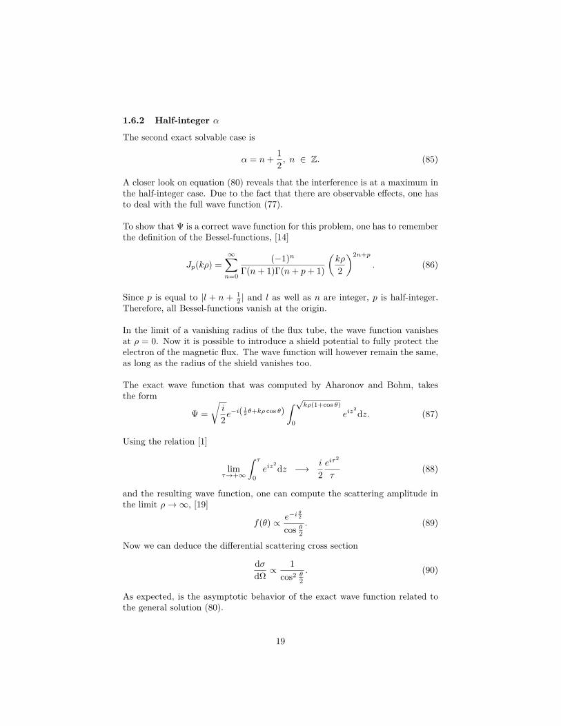
1.6.2 Half-integer α

The second exact solvable case is

α = n+ 12 , n ∈ Z. (85)

A closer look on equation (80) reveals that the interference is at a maximum inthe half-integer case. Due to the fact that there are observable effects, one hasto deal with the full wave function (77).

To show that Ψ is a correct wave function for this problem, one has to rememberthe definition of the Bessel-functions, [14]

Jp(kρ) =∞∑n=0

(−1)n

Γ(n+ 1)Γ(n+ p+ 1)

(kρ

2

)2n+p. (86)

Since p is equal to |l + n + 12 | and l as well as n are integer, p is half-integer.

Therefore, all Bessel-functions vanish at the origin.

In the limit of a vanishing radius of the flux tube, the wave function vanishesat ρ = 0. Now it is possible to introduce a shield potential to fully protect theelectron of the magnetic flux. The wave function will however remain the same,as long as the radius of the shield vanishes too.

The exact wave function that was computed by Aharonov and Bohm, takesthe form

Ψ =√i

2e−i( 1

2 θ+kρ cos θ)∫ √kρ(1+cos θ)

0eiz

2dz. (87)

Using the relation [1]

limτ→+∞

∫ τ

0eiz

2dz −→ i

2eiτ

2

τ(88)

and the resulting wave function, one can compute the scattering amplitude inthe limit ρ→∞, [19]

f(θ) ∝ e−iθ2

cos θ2. (89)

Now we can deduce the differential scattering cross section

dσdΩ ∝

1cos2 θ

2. (90)

As expected, is the asymptotic behavior of the exact wave function related tothe general solution (80).

19

1.7 Single-valuedness of ΨIn previous sections we calculated solutions for problems, implying excluded fluxregions, though spared an important issue: Is the solution of the Schrödingerequation still meaningful if it is computed in regions, where parts of space aremissing?

Requiring a vanishing wave function in the flux region is strongly associatedwith excluding regions that are in the domain of the wave function. That leads,mathematically spoken, to a multiply-connected region. As we have seen in pre-vious sections, the wave function gains a phase by propagating in such regions.

That the initial wave function

Ψ = e−ikρ cos θe−iαθ (91)

is multivalued, can easily be shown by leading the wave function one time ona circuit around the excluded soleniod. [3] The change of the wave function istherefore

e−i2πα. (92)

It vanishes only if α is integer and from that follows the wave function is auto-matically single-valued. Since (90) is in general not a useful wave function it, isreasonable to consider this special case only.

For the second exact solvable case, α is half-integer, the wave function is alsosingle-valued. [1] This property is not as obvious as in the first case. The rea-son for single-valuedness is the asymptotic behavior of (87). It is the same asthe general solution (79), for half-integer flux parameter α, as shown in section1.6.2. [19]

Generally, it is important to note that due to the single-valuedness of the Hamil-tonian, the single-valuedness of a wave function is preserved. If a wave functionis single-valued in the first place (in our case far from the origin), this propertycannot be changed. [2]

20

2 AB-Effect: Experiments2.1 Chambers [4]A few months after Aharonov and Bohm published their first paper, Robert G.Chambers realized the first experiment focusing on the AB-effect. The follow-ing experimental set-up was used: A and B denote the different electrodes of

Figure 4: Chambers’ interference experiment [4]

an electron-biprism, which was used to focus the electrons to the observationscreen. The electrodes A are used as groundings, whereas B provides a pos-itive potential that determines the angle of deflection. In the shadow of B amono-crystalline iron filament, with a diameter of 1 µm, is arranged. This so-called iron whisker [23] is partly conical and partly cylindrical and provides themagnetic flux. Since the magnetic domains in this whisker are uniform, the flux

Figure 5: Tilted fringes causedby conical whisker [4]

direction is well-defined. [19]

Further it is interesting to note that thewhisker tapers approximately constant witha slope of 10−3 rad. Stressing thisfact and the uniformity of the magneti-zation, one finds that the enclosed fluxdecreases with the length of the filamentThis means that the phase of the elec-trons depends highly on the point of pass-ing. [18]

Additionally, it is known that the magneticlines exit the tapered parts of the whisker per-pendicular to the surface. Therefore, a strayfield exists, which tilts the interference fringesproportionally to the flux change. Addition-ally to the tilt, the fringes are continuouslyconnected. This holds if the phase shift exists in the cylindrical regime too. [19]

In conclusion it has to be mentioned that there has been criticism too. Aharonovand Bohm stated that the use of whiskers does not provide a solid proof of theAB-effect, since ~A and ~B are not separated adequately. [2]

21

2.2 Möllenstedt and Bayh [16]In 1962 the second remarkable experiment was carried out by G. Möllenstedtand W. Bayh. They used a similar set-up like Chambers, as can be seen inFigure 4, but in contrary a thin solenoid was used to generate the magneticflux. To minimize the leakage fields, a Fe/Ni-frame was added to the solenoid,

Figure 6: Interference experiment of Möllenstedt and Bayh, [16]

which was made of tightly wound Wolfram-wire. The purpose of such a frame,was to short-circuit the magnetic field on the ends of the solenoid. Furthermore,they stated that such a set-up is preferable to the use of whiskers, because theflux is not fixed to the filament. This property was stressed to visualize theconsequences of the vector potential.

As the solenoid current was increased up to 0.8 µA, a film was moved pro-portionally to the current change. The outcome of the experiment is shown inFigure 5, where the fringe shifts, which appear due to the vector potential, arevisible. The analysis of the experiment confirmed furthermore the modulus ofthe flux quantum

φ0 = 4.07 × 10−7Gcm2 ± 14%.

Figure 7: Interference pattern with fringe shifts [16]

22

2.3 Tonomura et al. I [5]The next experiment was carried out in 1982 by Akira Tonomura et al. Theychose a different set-up as Chambers or Möllenstedt and Bayh, namely optical-and electron-holography. This technique consists of two parts, an electron mi-croscope and an optical system, which transforms the electron waves into light

Figure 8: Set-up for electron holography[5]

Figure 9: Set-up for Reconstruction ofelectron hologram [5]

Figure 10: Interference pattern of thetorus. (a) Contour map of the electronphase. (b) Interference pattern of theelectron phase [5]

waves. [22] In Figure 8 the set-ting for the electron microscope issketched. In the case of the ac-tual experiment, the "Specimen" isrealized by a toroidal Fe/Ni-alloy,with an outer radius of about 1µm. The advantage of a toroidalshaped magnet, is the reduction ofleakage fields. Since the magne-tization could be orientated clock-wise or counterclockwise, the fluxis by approximation confined to themagnet. More precisely, one of theconsequences of this experiment wasshowing that the leakage fields weretoo small to affect the AB-phase.Figure 9 shows the second part ofthe set-up, which was used to recon-struct the electron hologram. Thebeams were provided by a He-Nelaser and then split coherently intotwo beams. The first beam picturesthe hologram of the toroidal mag-net, whereas the second was usedas "reference" to get the interferencepattern. Since this method onlymagnifies the signal, the amplitudeand phase of the electron wave isconserved and the image of the torusis meaningful. [22]Figure 10 shows an image of thetorus, using two different methods.(a) is a so-called contour map ofthe electron phase, which was cre-ated by plane light wave parallel tothe electron wave. It represents themagnetic lines inside the toroidalmagnet. (b) on the contrary dis-plays the interference pattern of theelectron wave.

23

It shows the gained phase shift, due to the vector potential. This method isslightly different to the contour mapping. The electron hologram is imaged bya wave front, which is not parallel to the object wave. [22]

Figure 11: [22]

Shown are these differingtechniques in Figure 11, wherethe labels match with Figure10. This problem is compa-rable with a photograph of amountain, where (a) is takenfrom above and (b) of theside. [22]

To summarize the first ex-periment of Tonomura et al.,they showed that there exists a measurable effect due to the vector potential,because the electron waves that passed on different sides of the magnet, gaineda visible phase difference. Furthermore, they performed a reasonable analysis ofleakage fields and stated that the effect is too small to influence the interferenceexperiments. [5]

2.4 Tonomura et al. II [6]For further observation of the AB-effect, Tonomura et al. did a rerun of theirexperiment in 1986. Instead of using a bare toroidal magnet, they covered itwith superconducting material, namely Niobium (Figure 12). By using such aset-up, they stressed the Meissner-Ochsenfeld-effect to increase the precision.

Figure 12: Diagram of the magnetstructure [6]

Due to circulating currents in lay-ers near the surface, the magneticfield cannot fully penetrate the su-perconducting materials, if they arecooled under their critical temper-ature. [15] The consequences aretwofold: on the one hand, the flux isconserved to the Fe/Ni-alloy and noleakage fields can influence the elec-tron waves and on the other hand,the magnet is completely shielded bythe Niobium, so the electrons can-not enter the regime of the Fe/Ni-torus.

Furthermore, it is interesting to visualize the thickness of the toroidal magnet.In Figure 12 it can be seen that the structure contains a SiO- and a Fe/Ni-layer.

24

The alloy is 20 nm, whereas the Silicon Monoxide-layer is 50 nm thick. Enclosedare these rings by 250 nm of Niobium and further by a additional 100 nm Cu-cover. Due to the approximated penetration depth of the electrons of 110 nmin Nb, it is very important to add further covering of the flux, to minimize theeffects of leakage fields. They stated that at room temperature the magnitude ofthe leakage fields is of the order of approximately h/20e. Therefore, it is reason-able to assume the leakage fields at working temperature ( 300K) much lower.

To conclude this section, it is interesting to analyze interferograms (see Fig-ure 11) of the magnet.

Figure 13: Interferogram of the toroidal magnet, T = 4.5K [6]

In Figure 13 the phase shift of the electron waves is visible. The electrons, whichpass through the hole of the torus, gain a different phase than the ones, whichpass on the outside. This is indicated by the dashed line.

One more time Tonomura et al. observed phase shifts, but under tightenedconditions, compared to the experiment in 1982. Furthermore, they stated thatthe phase shift shown in Figure 13 is a multiple of π. This is an indication forflux quantization proportionally to hc/2e. (see equation 60)

25

3 Quantum Interference devices3.1 AB-Effect in ring structuresIn previous sections, we analyzed theoretical concepts, respectively experimentalset-ups and noted the largeness of the particular electron microscopes or opticalsettings. An approach - not untypical for modern physics - is to minimize theexisting structures and examine the consequences. That leads to the simplesttoy-model, the Aharonov-Bohm-ring [AB-ring].

Figure 14: Experimentalrealization [17]

Figure 15: AB-ring [17]

Figure 14 shows an actually realized ring structure, where the black domainsrepresent electron reservoirs. Figure 15 on the other hand, shows a sketch of anAB-ring, where the black colored triangles denote ideal beam splitters, whichare described by a scattering matrix. Further, it is evident in the figure thattwo different phases are applied to the wave function if it passes trough on ofthe arms of the ring. χi is a dynamical phase, due to the device, and φi (i =1,2) a magnetic phase, due to the flux. Since we consider only ideal rings, it isjustified to choose χ1 = χ2 = χ/2. [17]

For computing the transmission amplitude T, in fact every possible trajectorythrough the ring has to be counted. Considering only trajectories with a maxi-mum of one loop, we end up with

T = (1− cosχ)(1 + cosφAB)sin2 χ+ [cosχ− (1 + cosφAB)/2]2

, (93)

where φ1 + φ2 = φAB ≡ e~cφ = π φ

φ0. [60] Using equation (93), it is possible to

compute the conductance of an AB-ring. Generally, this is given by

G = GQT (χ, φAB) = e2

π~T (χ, φAB), (94)

where GQ is the conductance quantum. Summing up the last results, it followsthat the conductance of the AB-ring alters periodically with φ0 and therefore theresistance alters too. [17] This statement has been proven by many experimentswith AB-like [17] and graphene rings. [7]

26

References[1] Y. Aharonov and D. Bohm. Significance of electromagnetic potentials in

the quantum theory. Physical Review, 115(3):485, August 1959.

[2] Y. Aharonov and D. Bohm. Further considerations on electromagneticpotentials in the quantum theory. Physical Review, 123(4):1511, August1961.

[3] M.V. Berry. Exact Aharonov-Bohm wavefunction obtained by applyingDirac’s magnetic phase factor. European Journal of Physics, 1:240–244,1980.

[4] R. G. Chambers. Shift of an electron interference pattern by enclosedmagnetic flux. Physical Review Letters, 5(1):3–5, July 1960.

[5] A. Tonomura et al. Oberservation of Aharonov-Bohm effect by electronholography. Physical Review Letters, 48(21):1443, May 1982.

[6] A. Tonomura et al. Evidence for Aharonov-Bohm effect with magnetic fieldcompletely shielded form electron wave. Physical Review Letters, 56(8):792,February 1986.

[7] J. Schelter et al. The Aharonov-Bohm effect in graphene rings.arXiv:1201.6200 [cond-mat.mes-hall], January 2012.

[8] M. Peshkin. et al. The quantum mechanical effects of magnetic fields con-fined to inaccessible regions. Annals of Physics, 12(3):426–435, 1961.

[9] B. Felsager. Geometry, Particles and Fields. Odense University Press, 2edition, 1983.

[10] R. Feynman. Quantum Mechanics, volume 3. Basic Books, 2010.

[11] T. Fliessbach. Mechanik. Spektrum, 6 edition, 2009.

[12] T. Fliessbach. Elektrodynamik. Spektrum, 6 edition, 2012.

[13] D.J. Griffiths. Introduction to Quantum Mechanics. Prentice Hall, 1995.

[14] C.B. Lang and N. Pucker. Mathematische Methoden in der Physik. Spek-trum, 2 edition, 2010.

[15] D. Meschede. Gerthsen Physik. Springer-Verlag, 24 edition, 2010.

[16] G. Möllenstedt and W. Bayh. Kontinuierliche Phasenverschiebung vonElektronenwellen im kraftfeldfreien Raum durch das Vektorpotential einesSolenoids. Physikalische Blatter, 18(7):299–305, Juli 1962.

[17] Y.V. Nazarov and Y.M. Blanter. Quantum Transport: Introduction toNanoscience. Cambridge University Press, 2009.

27

[18] S. Olariu and I. Iovitzu Popescu. The quantum effects of electromagneticfluxes. Reviews of Modern Physics, 57(2):339–433, April 1985.

[19] M. Peshkin and A. Tonomura. The Aharonov-Bohm Effect. Springer-Verlag, 1989.

[20] J.J. Sakurai. Modern Quantum Mechanics. Addison-Wesley PublishingCompany, revised edition edition, 1994.

[21] F. Schwabl. Quantenmechanik. Springer-Verlag, 7 edition, 2007.

[22] A. Tonomura. Electron Holography. Springer, 2 edition, 1999.

[23] Online version of McGraw-Hill Encyclopedia of Science and Technology.

28