the role of forestry in carbon sequestration in general
TRANSCRIPT
The Role of Forestry in Carbon Sequestration in General Equilibrium Models *
by
Brent Sohngen1, Alla Golub2 and Thomas W. Hertel3
GTAP Working Paper No. 49 2008
1Department of Agricultural, Environmental, and Development Economics, Ohio State University, 2120 Fyffe Rd., Columbus, OH 43210, Contact: [email protected] 2Center for Global Trade Analysis, Purdue University, West Lafayette, IN 47907: [email protected] 3 Center for Global Trade Analysis, Purdue University, West Lafayette, IN 47907: [email protected] *Chapter 11 of the forthcoming book Economic Analysis of Land Use in Global Climate Change Policy, edited by Thomas W. Hertel, Steven Rose, and Richard S.J. Tol

2
Table of Contents 1. Introduction ..................................................................................................................3 2. The Economics of Forest Management Under Carbon Policies ..................................5 3. Examples From a Global Timber Model ....................................................................16 4. Implications for CGE Modeling .................................................................................22 5. Evaluation of Current Approaches to Forestry Modeling in Global CGE Analysis ..27 6. Conclusion ..................................................................................................................30 7. References ..................................................................................................................33
Table 1. Carbon intensity in temperate zone forests (t C/hectare), expressed relative to the baseline carbon intensity (1.0 = no change) .........................35 Table 2. Annual equivalent carbon gains (losses) and production impacts over 20 years at three different carbon prices .............................................36 Figure 1. Proportion of carbon sequestration in temperate and tropical forests resulting from forestry actions for several different carbon prices over a 20 and 100 year period .............................................................................37 Figure 2. Biomass and Merchantable timber yield functions for upland hardwoods in the U.S. south ..........................................................................................38 Figure 3. Growth rate and average annual flow of timber from upland hardwood type in the Southern U.S. .............................................................................39 Figure 4. Present value of upland hardwoods in U.S. South under baseline (no carbon incentive) and three alternative carbon prices (derived from equation 5), assuming management inputs remain $56/hectare ..................40 Figure 5. Relationship between $/hectare management inputs, "n", and stocking density (delta, or δ) ......................................................................................41 Figure 6. Age class distribution of upland hardwood stands in the Southern U.S. in the baseline and climate mitigation scenario (high damage) from Sohngen and Mendelsohn (2006) ................................................................42 Figure 7. Aboveground carbon stored in natural southern pine stands in the United States in the baseline and the high damage carbon mitigation scenario .....43 Figure 8. Timber price index for baseline and high damage carbon policy scenario, derived from Sohngen and Mendelsohn (2007) ...........................44 Figure 9. Annual timber harvests in southern upland hardwood stands in the United States in the baseline and the high damage carbon mitigation scenario ........................................................................................................45

3
THE ROLE OF FORESTRY IN CARBON SEQUESTRATION IN GENERAL EQUILIBRIUM MODELS
Brent Sohngen, Alla Golub and Thomas W. Hertel
1. INTRODUCTION
The role of forestry in the global carbon balance is widely recognized, as described in
chapter 31. A number of models and methods have now been developed to assess the
potential role of forestry in climate mitigation policy (e.g., Adams et al., 1999; Stavins,
1999; Sohngen and Mendelsohn, 2003; Richards and Stokes, 2004). These studies
suggest that forestry could provide 1.0 – 2.0 Pg C/yr in sequestration services or avoided
emissions through reductions in deforestation for $150 - $200/ t C, amounting to
potentially one-third of efficient global carbon abatement (Sohngen and Mendelsohn,
2003). Given that these prices are well within the range of expected prices associated
with fairly stringent carbon abatement policies (see Weyant et al., 2006), current
economic analysis suggests that forestry can compete effectively with other mitigation
options. However, most of these studies of forestry’s role in climate change policy have
been partial equilibrium analyses that have ignored the broader implications of climate
policy on economic activity. As this book suggests, it is useful to develop general
equilibrium modeling frameworks that capture the full range of implications of climate
policies on carbon markets and consequently forest carbon sequestration activity.
The chapters in this book show that the state of the art in modeling forestry
activities within a general equilibrium context has advanced significantly in recent years.
Modeling carbon sequestration in forests within a general equilibrium context, however,
1 GTAP Working Paper No. 41

4
remains a formidable task because of the complex dynamic considerations inherent in the
economics of managing and modeling forests. While other land uses, such as agriculture,
may be modeled within the context of a comparative static, single representative time
period, or perhaps in the context of a recursive, dynamic model, forest management
involves investments in one time period based on expectations about what will happen
many years ahead. In terms of carbon sequestration, the carbon or timber benefits of
expenditures on forestry may not accrue for a number of years, presenting difficulties for
conducting static (single period) analysis in computable general equilibrium (CGE)
models. If CGE modelers instead utilize recursive models, forestry remains difficult to
incorporate because of difficulties in capturing the intertemporal management of forest
carbon.
In order to provide an economic basis for incorporating forestry management and
carbon sequestration into CGE models, this chapter explores the intertemporal forestry
management problem in some depth, thereupon providing information and insights that
may aid CGE modelers in developing improved representations of forestry in the context
of global climate policy analysis. The chapter begins with a description of the forestry
management problem, and illustrates how carbon sequestration incentives influence
forest management. The results of a global forestry model are then used to show the
importance of capturing the management effects in particular regions. The chapter then
briefly discusses the influence of other management options on forest carbon. Since one
of the most important effects of carbon policy on forestry may be changes in optimal
rotation lengths, one section of the chapter describes how CGE modelers may incorporate

5
short and longer term adjustments in age classes in their models. A brief evaluation of
how the models in this book capture forestry concludes the chapter.
2. THE ECONOMICS OF FOREST MANAGEMENT UNDER CARBON POLICIES Modeling carbon sequestration in forestry requires the assessment of changes in
management, rotation ages, set-asides, forest products, land use. Each of these concepts
requires some further clarification. Changes in forestry management include actions like
thinning, fertilizing, herbicide treatments, pruning, planting, and replanting. Changes in
rotation ages are also a form of management change, but are usually considered
separately from other management actions. Set-asides refer to removing timberland from
the active forest management base and holding the land as a carbon reserve. Forest
product storage refers to the storage of carbon in marketed products. For example, many
sawnwood products will ultimately be used in construction (e.g., to build houses), or in
furniture. These products have long-lives, and during their lives the carbon in the wood
products is with-held from the atmosphere. Finally, changes in land use, including
afforestation (planting lands that were previously in agriculture) and reductions in
deforestation (keeping lands in forests that would otherwise convert to agriculture) are
two potential options for carbon sequestration that have been widely discussed in the
policy arena.
The economic efficiency of choosing among these sequestration options in any
particular region of the world will depend on the relative costs of implementing the
actions versus the benefits (e.g., carbon sequestered). Both costs and carbon intensities

6
vary substantially across regions. Chapter 32 provides information on both the biological
growth and the economic parameters that can be used to assess forestry actions in
different regions. To get a sense for the relative size of carbon storage available from
different types of activities, estimates of the proportion of carbon sequestered or
emissions reduced across different activities in temperate and tropical forests for several
carbon prices are shown in Figure 1.3 These estimates are derived from the model used
in Sohngen and Mendelsohn (2007), which determines an "optimal" allocation of carbon
sequestration in different activities and time periods given a constant carbon price over a
20 year, and 100 year period, respectively.
As can be seen in Figure 1 (panels A & B), in the short run (i.e., over the next 20
years), most carbon sequestered in temperate forests will be obtained through extending
rotation ages, changing management, and setting aside forests. By contrast, in tropical
forests, nearly all the short run carbon sequestration is obtained from reduced
deforestation. In the longer-run (Figure 1, panels C & D), afforestation plays a more
important role in temperate zones, although in terms of annual equivalent amounts, it
remains less than 30% of total temperate forest sequestration for the range of carbon
prices considered. Afforestation, and in particular reductions in deforestation, remain
dominant components of overall carbon sequestration activities in tropical forests, even
over the long run.
The example in Figure 1 illustrates the importance of understanding how carbon
is sequestered in forests and through forestry activities when implementing forest carbon
2 GTAP Working Paper No. 41 3 Reductions in carbon emissions from avoided deforestation are described as "emissions reductions" in this paper, while increased carbon stored in forests through rotation changes, management changes, afforestation, etc. is described as "carbon sequestration in this paper.

7
sequestration in CGE models. Given the relative importance of age class management,
the results suggest that it is as important to model what happens to the distribution of age
classes (e.g., the rotation age) as it is to model what happens to the total area of forest
land. To assess the implications of carbon prices on forest rotation ages and forest
management, this section considers these two activities in the context of a simple, single
hectare, forestry management model. Later in this chapter, we use a global timber model
to expand these results to the regional level.
Modeling forestry rotation ages and management begins with modeling the yield
of biomass and merchantable forestry products. Forest yield functions have the typical
logistical shape identified with most biological species. Equation (1) presents the
biomass growth function for upland hardwoods in the Southern U.S. region, which
translates the age of the stand into the cubic meters of biomass on the site:
(1) VaC (m3/ha) = δ*exp[5.2 – 30/(age)]
The parameter δ captures stocking density, which will typically range from 0.6 to 1.4,
depending on average management inputs in a region. Stocking density is a unitless
parameter that adjusts the yield function for average conditions of specific sites or
regions. Stocking density can be assumed to be given exogenously, or it can be assumed
to be an endogenous function of management inputs. Initially, we assume that stocking
density, δ, is exogenous.
As forests age, the value of the merchantable component of the stock increases.
Bigger stems improve stand quality because more material can be utilized for sawtimber,

8
which is a higher value use of the material. To account for this improvement in value
over time, we utilize an additional function to depict the proportion of merchantable
timber on a given site (once the forest reaches the commercially viable vintage):
(2) γ(age) = 0.85*[1-exp(1-0.1*(age-30))]2
The merchantable yield for this southern upland hardwood forest type becomes:
(3) if age ≤ 30 => 0
If age > 30 => VaM (m3/ha) = γ(age)*δ*exp[5.2 – 30/(age)]
Figure 2 shows biomass yield and merchantable yield for particular forest type.
As can be seen in equation (2), merchantable yield can be at most 85% of the biomass in
growing stock on the site. Furthermore, with equation (3), we have assumed that there is
no merchantable yield before age 30. These are both strong assumptions which may be
violated at particular sites where timber operations occur, however, when aggregated
across a large number of sites (i.e., a region), the assumption is more realistic.
In a static world, the harvest age occurs where the net present value of the stand is
maximized. The net present value of a single rotation when prices are held constant is:
(4a) NPVT = CrVP aMa
QA −+ −)1)((*)( ,
and the net present value of an infinite series of rotations when prices are held constant is:

9
(4b) NPV∞ = ))1(1()1)((*)(
a
aMa
QA
rCrVP
−
−
+−−+
In equations (4a) and (4b), PQA is the quality adjusted stumpage price for timber, r is the
interest rate, C is the planting or regeneration cost, and "a" is the rotation age. Planting
costs (investments) occur at the beginning of the rotation, and the benefits of harvests
occur when trees are harvested at time "a". The quality adjustment factor accounts for
any quality differences associated with particular timber types that are found in local or
national price data. The rotation age can be determined endogenously by maximizing (4)
with respect to "a". If timber prices are $100/m3, replanting costs are $56/hectare,
δ=1.15, and r=0.05, the optimal rotation age in this case will be a = 48 years, the biomass
yield will be 112 m3/ha and the merchantable yield will be 66 m3 per hectare. The net
present value of the stand will be $642/hectare. For simplicity, assume that the rotation
age is rounded to 50 years old. If there are 34 million hectares of this type of land, then
on average 0.68 million hectares will be cut each year, or 45 million m3 per year
(0.68*66).
A number of important relationships can be analyzed with the yield function and
net present value formula shown in equations (1) – (4). First, the optimal rotation age
occurs approximately at the point in time when the value of the stand, (PQA)*(VMa), is
growing at the rate of interest, which translates (with constant prices) into the time when
the stand itself is growing at the rate of interest. Since the interest rate in this case is 5%,
the stand is growing at approximately 5% per year at 50 years, which is the optimal
rotation length. Note that this optimal rotation period is not the same time interval as that

10
which maximizes the flow of timber from the land. That age, often called "maximum
sustainable yield," occurs later, as shown in figure 3, which displays the annual
percentage growth rate and the annual average flow of timber from this stand of forest.
The annual average flow of timber is calculated as the merchantable yield divided by the
age. Maximum sustainable yield in this type of forest occurs at age 60, or 10 years later
than the optimal rotation age. The profit maximizing rotation period is shorter due to the
opportunity cost of forestry investment, as reflected in the discount rate.
For further insight, let us consider the case wherein this type of forest is harvested
every 60 years. The merchantable yield of a 60 year old stand, by equation (3) above is
97 m3 per hectare. If rotations are 60 years in length, then 0.57 million hectares of the 34
million hectares will be harvested each year. This is fewer hectares than with the 50 year
rotations, but more timber is harvested on each hectare (97 m3 for the 60 year old stand
versus 66 m3 for the 50 year old stand). By waiting 10 years, one has obtained 53% more
merchantable timber, and the area harvested each year has only gone down by 16% (0.68
million hectares/yr down to 0.57 million hectares/yr). The annual flow of timber could
be 55 million m3 per year (0.57*97) if harvested at the maximum sustainable yield age of
60 years. But commerical forests that are not harvested at maximum sustained yield
because the additional 10 years of waiting impose substantial opportunity costs. Once
these opportunity costs are taken into account, one will move to shorter rotations.
There a number of reasons why managers might move towards harvesting older
age classes. Some governments, for instance, impose minimum rotation ages that are
above the economically optimal rotation ages. There may be several explanations for
this. Countries that have extensive government holdings may be interested in
11
maximizing their annual revenues rather than their land value, so the contracts they sign
with harvesters are likely to emphasize maximizing annual harvests. Alternatively,
countries may choose to impose environmental constraints that lead to longer rotation
ages on government or private lands. From an economic perspective, harvesting stands
in older rotation ages can make sense if there are non-market benefits associated with
older aged stands (see, for example, Hartman, 1979). A different rationale for
lengthening the rotation period relates to interest rates. Binkley (1987) has shown that
harvests move towards maximum sustained yield when interest rates fall. So if the
government believes that the discount rate used by the forest managers is too high, they
might wish to lengthen the rotation period. Carbon sequestration offers another reason
for lengthening rotations, since the sequestration benefits increase in direct proportion to
the yield of timber (Van Kooten et al., 1995). Indeed, this is the dimension of optimal
rotation length that is of greatest interest in the context of the present chapter.
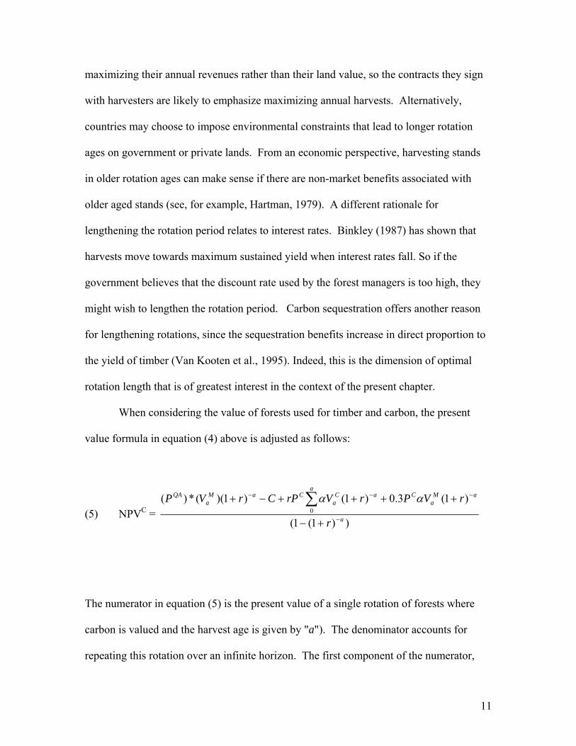
When considering the value of forests used for timber and carbon, the present
value formula in equation (4) above is adjusted as follows:
(5) NPVC = ))1(1(
)1(3.0)1()1)((*)(0
a
aMa
Ca
aCa
CaMa
QA
r
rVPrVrPCrVP
−
−−−
+−
++++−+ ∑ αα
The numerator in equation (5) is the present value of a single rotation of forests where
carbon is valued and the harvest age is given by "a"). The denominator accounts for
repeating this rotation over an infinite horizon. The first component of the numerator,

12
aMa
QA rVP −+ )1)((*)( , is the present value of timber benefits where PQA is the quality
adjusted price of timber stumpage, VaM is the merchantable timber harvested at age "a",
and (1+r)-a is the discount factor, where "r" is the discount rate. The second term, C, is
the cost of replanting. The third term, aa
Ca
C rVrP −+∑ )1(0
α , is the rental value of holding
carbon during the rotation. PC is the carbon price, and rPC is the carbon rental value.
Note that we assume carbon prices are constant in this case. The term α is in Mg C per
m3 of wood. VaC is the biomass yield function described above. The final term is the
value of permanent storage of carbon in harvested timber products. For this analysis, we
have assumed that 30% of wood is permanently stored. This present value formula will
allow modelers to determine the value of land in which produces jointly commercial
forest products as well as carbon storage. If this value outweighs the opportunity costs of
using the land for agricultural products, then in principle, the land should shift to forestry.
Carbon incentives have a number of impacts on forestry activity. First, they affect
the value of land in forests. Figure 4 shows the net present value (bare land value) of
forestland in the baseline (no carbon prices) and three carbon prices: PC = $50, $100, and
$200 per t C.4 The value of land in forests rises from $642/ha in the baseline, to
$4859/ha when carbon prices are $200/t C. At $4859/ha, forests can compete strongly
with other uses, such as crops. Of course, these values apply only to upland hardwoods,
which have fairly high carbon intensity per hectare (Sohngen and Brown, 2006), but
nonetheless, high carbon values would have strong impacts on how much land is
maintained under forest cover. Second, carbon prices extend rotation ages. The rotation
4 Note that for this analysis we have assumed that management inputs are held constant. As shown below, management inputs would change with carbon policy, and so one would expect optimal responses to differ from the examples with carbon prices in this section.

13
age is increased from 50 to 60 years of age with the $200/t carbon incentive. This can
effect is also evident in figure 4 wherein the maximum land value shifts to the right as
carbon prices rise.
In summary, carbon incentives have strong implications for the value of land in
forests and non-negligible implications for rotation ages. Each timber type (and
landowner or manager) will react differently to carbon prices, depending on the shape of
the growth function, interest rates, timber prices, costs of regenerating, and carbon prices.
Higher carbon prices increase land values in forestry and extend rotations. Longer
rotations increase the supply of timber from forests in the long-run because they move
forests closer to maximum sustained yield. At some carbon price, however, it may be
optimal to simply set-aside forests because they are more valuable as carbon reserves
than as harvested timber forests. There are thus two caveats to the implications of
rotation extensions for commercial timber supplies. First, in order to extend rotations, one
must choose not to harvest forests. Therefore, in the short-term, the effect of the carbon
subsidy is to reduce timber supply. A market model would respond to this short-term
reduction in supply by increasing timber prices. Second, in the long-run, if carbon prices
rise substantially, some forests may be converted to carbon reserves and never harvested.
Creation of carbon reserves will serve to reduce timber supply in the long-run, which will
tend to counteract the effect of moving towards the maximum sustainable yield. In
summary, the impact of carbon prices on commercial forest supplies is complex. In fact,
it is even more complex than this, since we have not yet considered the impact of carbon
prices on management intensity. We now turn to this issue.

14
The Effect of Carbon Prices on Timber Management: As shown in figure 1, forest
management activities beyond changes in rotation ages potentially provide 20 – 30% of
forest carbon sequestration across carbon prices ranging from $10 - $100/t C. The
analysis above, however, focused solely on age class management. Other types of forest
management activities include replanting more intensively, thinning, fertilizing, using
herbicide treatments, and other actions. Incorporating management intensity adjustments
into CGE models will impose additional demands on CGE modelers. In order to inform
researchers seeking to capture this dimension of the intensification response to higher
carbon prices, this section describes how management intensity is captured in the global
timber supply model of Sohngen and Mendelsohn (2007).5
Sohngen and Mendelsohn (2007) handle management actions via the stocking
density parameter, δ. Instead of treating it as exogenous, as was done above, here we
assume that it is a function of management inputs. Stocking density is written as:
(6) δ = 0.8*(1 + C)n .
In equation (6), C is the planting cost, 0.8 is the value of δ without management inputs
(the un-managed natural yield), and "n" is an elasticity parameter of stocking density with
respect to management input. In the Southern upland hardwood example above, "n" is
assumed to be 0.09. If planting costs are $56 (as assumed above), then δ = 0.8*(1 +
56)0.09 = 1.15.
One can see the influence of management inputs (C, or $/hectare) and the
parameter "n" in Figure 5. Increases in management inputs increase the stocking density 5 Obviously there are other options for incorporating management intensity decisions into such models.

15
of forestland, although the marginal cost of boosting yields is increasing in C (Figure 5).
We expect the shape of this marginal cost function to vary by species of tree. Fast-
growing plantations, for example, are often more responsive to adjustments in
management, and thus may be assigned a higher value for "n". In Figure 5, we plotted
three different yield functions for three levels for "n" used in the global timber model.
The highest level, n = 0.13, suggests relatively large potential to increase management.
Species that are less responsive to management inputs are assigned a lower level for "n",
with the least responsive species being given the value of 0.05.
For simplicity, equations (4) and (5) were not solved for C when they were
introduced above, however, since δ is a function of C, equations (4) or (5) can be
optimized for C at the same time they are optimized for rotation age. The $56/hectare
management input is the optimal management input under baseline timber prices with no
carbon values. In the baseline, with this management effort, the net present value of the
stand is $642/hectare. If management inputs are increased by $10/hectare to $66/hectare,
the present value of the stand falls to $641/hectare. The additional costs increased output
at harvest time, but the value of these improvements were less than $10/hectare.
While it would not be profitable to expand management inputs beyond
$56/hectare in the baseline, management inputs would increase if a price is placed on
carbon sequestration. With a carbon price of $100/t C, the value of the stand is
$2702/hectare under a $56/hectare management level. However, under the $100/t C
carbon price, the optimal management input is $264/hectare, and the value of the stand is
$2887. Biomass in 48 year old stands initially will be 112 m3/hectare, but at $100/t C,
with management inputs of $264/hectare, biomass in a 48 year old stand will be 128

16
m3/hectare, or an increase of 15%. Thus carbon sequestration subsidies can have an
important impact on the intensity with which forests are managed, thereby inducing an
increase in forest product output.
3. EXAMPLES FROM A GLOBAL TIMBER MODEL
This section illustrates the single-stand responses discussed above by using the results
from the global timber model analysis conducted by Sohngen and Mendelsohn (2007).
That study developed a baseline case, and then explored a set of carbon policy scenarios.
One of the scenarios assumes relatively high damages from climate change. In their
"high damage" scenario, carbon prices start at $22/t C in 2005, and rise to $187/t C by
2105. This path of carbon prices reflects increasingly stringent emissions restrictions.
Because the model is global in scope, carbon prices influence forests and timber prices
globally. In this section, we focus on specific management activities in a single region of
the model. However, the results are cast in a global context.
Forest Carbon Response to Adjustments in Age Classes: Carbon sequestration is a
function of the inventory of forests, which in turn is a function of the age class
distribution. One of the most important responses landowners may make to carbon
incentives is to adjust the rotation age, particularly in the short-run when the area of
forests cannot be expanded. (Even if it could be expanded, new plantings would not
provide large quantities of carbon services for a number of years.) Extending rotations
would not appear to provide substantial carbon when considered on an incremental, per
hectare basis, but widespread adjustment in rotation ages across all commercially
harvested hectares in response to carbon incentives, can have important effects on the

17
total stock of carbon stored in forests for an entire region. Furthermore, because this is
just a marginal adjustment, it can be undertaken immediately by forest managers.
Therefore, as we have seen in Figure 1, changes in the age structure of the forest could
well account for the majority of the carbon sequestered in temperate forests in the near
term (e.g., 20 years), particularly at low carbon prices.
To examine the importance of accounting for changes in rotation ages on carbon
sequestration, consider the implications of carbon incentives on upland hardwood stands
of the Southern United States. Forests of the same type introduced in the previous
section are included in the global timber model of Sohngen and Mendelsohn (2007).
That model takes a dynamic optimization approach to managing stands by maximizing
the net present value of consumer and producer surplus in timber markets. In the baseline
case, the model ignores incentives for carbon sequestration. In the carbon policy scenario,
carbon sequestration is modeled by renting carbon in the standing stock of forests. The
model rents carbon along the high damage scenario price path introduced above.
Under the baseline, upland hardwood stands in the Southern U.S. region of the
model are "optimally" harvested in 50 year rotations. Panel A of Figure 6 shows that the
initial stock of Southern upland hardwood stands have a maximum age of 60 years (note
that we are only considering the timber forests in this example, not less intensively
managed forests that would already be at older rotation ages). In the baseline simulation,
these 60 year old stands are harvested in the first time period, and the stock is then
converted to a 50 year old stock in years 20 and 30 (Panels B and C, Figure 6) in order to
maximize net present value of the forestry activity on this land.

18
The carbon prices for the high damage scenario induce landowners with upland
hardwood stands in the U.S. South to hold timber longer than in the baseline (Figure 6).
Stands are held at 60 years of age through the 30th year of the simulation, in the presence
of carbon prices, whereas they decline to 50 years of age in the baseline. The total area
of forestland also increases by 2.1 million hectares by year 30 in the carbon policy
scenario, but the increase in forestland does not result primarily from additional planting
of forests. Indeed, in year 20 of the simulation, there is less stock in the initial age class
under the carbon policy scenario than in the baseline. The increase in forest land area is
due to the fact that the stands that would have been harvested at 50 years in the baseline
are now maintained in 60 year rotations in years 20 and 30, thus giving rise to an increase
in total forestland compared to baseline.
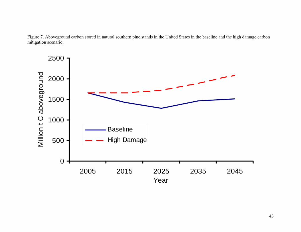
Figure 7 shows that increasing rotation ages by 10 years (from 50 to 60 years)
increases total carbon sequestered in natural southern pine forests over the 30 year time-
frame (assuming that the first decade starts in 2005). Total storage increases by 436
million t C by the 30th year of the simulation. This increase is attributed to an increase in
the rotation age, although the total forestland area has also increased by 2.1 million
hectares. Expanding rotations means that each of these additional hectares adds carbon
storage of 79 t C per hectare, far exceeding the average storage of carbon of around 49 t
C per hectare in these types of stands. This example illustrates why adjusting rotation
length is such a powerful vehicle for increasing forest carbon in the near term. Indeed, as
the intertemporal optimization model shows, in the first 30 years, it is far more efficient
than simply planting new stands and waiting for them to grow.
19
These results illustrate the importance of accounting for management of
timberland when measuring adjustments in carbon sequestration triggered by carbon
policy. Most computable general equilibrium (CGE) models that model forestry do not
optimize age class management over time. Therefore, they are unable to account for the
many adjustments that landowners can make to carbon sequestration incentives, as
captured in a dynamic model like Sohngen and Mendelsohn (2003, 2007). One exception
is the chapter6 by Sands and Kim in this volume, wherein the CGE model endogenizes
optimal rotation length via incorporation of a steady-state formula. This will be discussed
further below.
Of course, the results shown here also suggest the importance of accounting for
age class distributions – particularly if one wishes to track the path of adjustment from
one steady state to another. This is necessarily ignored in any formulation that deals only
with steady state outcomes.
Forest Product Response: Changing rotation ages will alter the flow of products
from the forest sector. Changes in timber supply, in turn, will affect prices, and hence the
efficiency of the carbon actions themselves. It is thus useful to consider the response of
timber markets to carbon incentives. This is particularly important in the case where
some regions do not participate in global policy (e.g., they have a $0/t C price). The
extent of leakage to non-participating regions now depends on what happens to global
forest product prices. And these price impacts in turn depend on supply changes from the
regions facing carbon prices. As seen above, product supply will depend on total hectares
forested, rotation ages and management intensity.
6 GTAP Working Paper No. 45

20
Forest product responses are likely to be quite large when carbon policies are
introduced. Figure 8 shows timber prices in the baseline and the high damage carbon
policy described above. In the carbon policy simulation, timber prices initially rise
around 1% compared to the baseline as global supplies are reduced. By 2045 they fall by
around 3% relative to the baseline. The carbon policy induces landowners to hold timber
initially, and thus capture carbon rents. In the longer run, additional land supply, higher
rotation ages, higher management, etc., increase the total timber supply, causing prices to
fall.
One can see the effects of the carbon policy more directly by analyzing the effects
on the Southern hardwood type described above. In year 20 of the baseline in the
example above, there are 4.9 million hectares of land at age 50. When age = 50 years
(the baseline rotation age in the model), the yield of merchantable timber would be 72
m3/ha. All of these hectares would be harvested, so over the 4.9 million hectares
harvested, timber supply that decade (data is provided in 10-year age classes) would be
351 million m3/decade, or 35.1 million m3/yr over the decade. In contrast, under the
climate policy, there are 5.0 million hectares in age class 60 in the 20th year. The yield of
timber for 60 year old stands is 96.7 m3/ha, so total timber harvests are 486 million
m3/decade, or 48.6 million m3/yr. Raising rotation ages increases total timber harvests by
moving forests towards their maximum sustainable yield.
This quantity, however, applies only to the 20th year of that simulation. A
dynamic forestry model will adjust harvest ages in response to present and future timber
prices, carbon prices, and opportunity costs. In order to extend rotation ages by the 20th
year, some timber must be withheld from markets in initial periods. This is illustrated in

21
figure 9, where harvests in this forest type are presented for the baseline and for the high
damage carbon policy scenario. Initially, harvests are lower in carbon policy scenario
than in the baseline because some timber is with-held from markets in order to extend
rotation ages with the carbon price. Over the longer run, rotations are extended and
forest areas expand, so harvests increase above the baseline scenario.
Response of Forest Management: Management inputs are determined
endogenously with timber prices and carbon prices in the global forestry model. As
carbon prices rise, timber management inputs also increase in order to increase the carbon
density on forested sites. These enhancements to management, as shown in Figure 1, can
provide substantial benefits in terms of carbon sequestration.
For the Southern hardwood forests discussed above, management inputs in the
baseline are approximately $56/hectare over the first 50 years of the simulation. With the
high damage carbon policy, however, these inputs triple in size in this type, to around
$170/hectare. Southern upland hardwoods currently experience a relatively low level of
management intensity overall, and these results indicate that there are efficient
opportunities to increase management and enhance carbon sequestration. This is a
relatively strong response. Species that are more intensively managed in the baseline,
such as Southern pine plantations, experience only 30% increases in management inputs
with the high damage carbon policy. This makes sense given that more intensively
managed species will already contain fairly high carbon stocks, and thus they are likely to
have limited opportunities to improve stocking conditions with positive carbon prices.
Combined Effects of Rotation and Management Changes: One way to gauge the
potential effects of both extensions in rotation ages and increases in the management

22
inputs is to assess the change in carbon on each hectare of land. These two activities have
their most pronounced and important effects globally in the temperate zones, so we focus
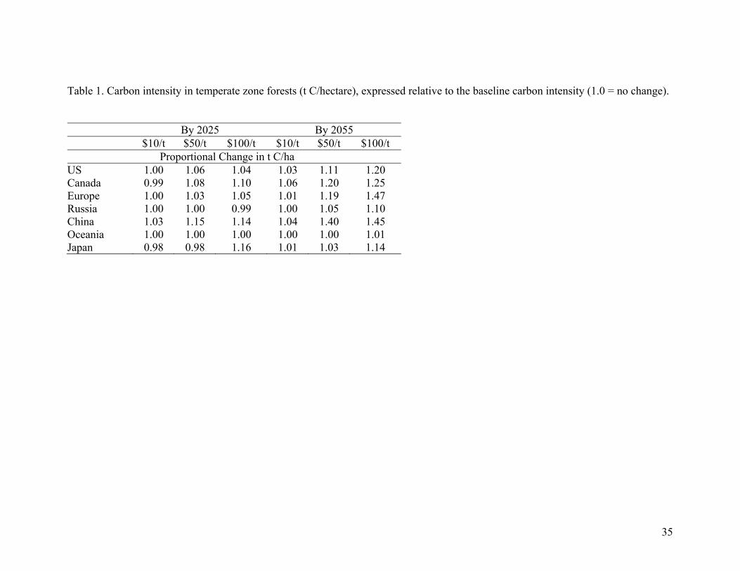
on that region for our discussion. Table 1 shows the ratio of average carbon intensity (t
C/hectare) for temperate forests for different constant carbon prices in the shorter term
(by 2025) and in the longer term (2055), relative to baseline. Thus an entry of 1.00 in
table 1 indicates no change under the carbon policy regime compared to the baseline.
These results suggest that carbon intensity rises on average as carbon prices rises.
Indeed, within the next 20 years or so, the global timber model suggests that, for a price
of $100/t C, carbon intensity in forests could be increased by up to 14% in China and
16% in Japan. And, if the same price were maintained in the future, over the next 50
years, carbon intensity could be increased by up to 47% in Europe and 45% in China,
with more modest rises in other regions. Of course these are the most responsive regions.
Oceania and Russia show very small responses on this intensive margin. 8667820900
4. IMPLICATIONS FOR CGE MODELING
Accounting for this potentially complex dynamic behavior in forestry can be
difficult in static or recursive dynamic CGE models. Fully intertemporal optimization
routines require substantial computing resources, which is particularly burdensome if the
interest of the modeler lies in the general equilibrium effects, since all sectors must then
engage in forward-looking investment behavior. For comparative static analyses, the
main issue becomes: Comparative static over what period of time? If the analysts are
primarily interested in long-run phenomenon, then they can potentially utilize steady-
state, static adjustments using a simple Faustmann model of optimal rotation. If, on the

23
other hand, analysts are interested in “near-term” phenomena – say the first 30 years -- it
will be fairly difficult to capture the dynamic effects described above. (We explore some
potential alternatives below.)
Assuming analysts are interested primarily in long-run effects, one way to handle
the rotation age adjustments that occur in forestry is to simply assume a uniform age
distribution and calculate the steady state effects based on comparing steady states (one
for the baseline and one for the carbon policy).With a uniform age distribution, the output
of interest is the average annual flow of forest product. Calculating average annual flow
is relatively straightforward. The modeler needs to obtain total hectares in the forest type
(summed over all age classes) and the optimal rotation age. In the example above, there
are 34 million hectares initially. If optimal rotations are 50 years, then 0.68 million
hectares will be cut each year on average (34/50). The yield at year 50 is 72.4 m3/ha, so
the average timber supply is 49.2 million m3/yr.
When carbon policies are introduced, two things must be considered: the change
in land area and the change in rotation ages. Changes in land area are best handled within
the CGE framework through a land market whereby forestry competes with other land
uses and land rents adjust to equate supply and demand for land of a particular
type/location. With carbon incentives, the value of forestland increases because the
standing stock of carbon has value. Since the forest land could otherwise be used for
other purposes, adding timberland has an opportunity cost. If carbon incentives draw
more land into forestry, modelers will need to adjust the average flow of timber from the
landscape. The value of land in forests when both timber and carbon are valued can be
estimated with equation (5) above. That equation provides the value of land in forests

24
under the carbon policy, and can be used as the relevant land value to be compared to
alternatives, such as agriculture.
Equation (5) can also be used to determine the rotation age of forests under a
carbon policy. As noted in the previous section, an increase in rotation ages increases the
long run supply of forest product. Under the carbon policy scenario described above, the
new optimal rotation age is 60 years. For the same 34 million hectares, average annual
flow under the 60 year rotation becomes 54.7 million m3/yr, which is larger than under
the baseline rotation of 50 years. This calculation of a change in timber production
assumes that the forest area has remained the same even under the climate policy.
Obviously, total forest area may change if the value of forests relative to other uses rises
due to the carbon incentives. In the example from the timber model described in the
previous section, over 100 years, forest area in Southern upland hardwoods increases to
46 million hectares. With 46 million hectares, the average annual flow of timber would
be 74.1 million m3/yr.
Finally, there is the question of stocking density. This is one area where CGE
models are relatively well equipped to deal with the forestry issue. The application of
additional inputs to a given unit of land to increase output per unit of land is analogous to
non-land/land substitution in the agriculture sectors of these models. Authors can either
employ equation (6) above, or they can calibrate the elasticity of substitution in a CES
production function involving land and non-land inputs to capture the same
intensification possibilities.

25
In summary, CGE modelers conducting static or recursively dynamic analyses of
long run policies must consider multiple factors if they hope to capture the key features
of forestry in climate mitigation analysis:
(A) Calculation of land values using equations (4) in the baseline or (5) under the
carbon scenario.
(B) Calculation of optimal rotation ages using equations (4) in the baseline or (5)
under the carbon scenario.
(C) Calculation of the optimal use of non-land inputs.
(D) Calculation of land areas using values obtained through (A) and comparing
those values to relevant values for other activities, such as agriculture.
(E) Calculation of average annual flow of timber.
Of course, by altering the supply of forest products, the change in annual timber flow will
have an impact on forest product prices as well. The extent of this change will depend on
the derived demand elasticity for output from the forestry sector. In a general equilibrium
model, this depends on the consumer demand elasticity for products like furniture,
housing, paper, etc., as well as the ability of the sectors producing these final goods to
substitute between other inputs and forest products.
As shown above, near term analyses create additional complexities for
incorporating forestry in CGE models. Carbon sequestration and timber production tend
to be complements in the long-run (expanding forest area, increasing forest carbon
through management, and increasing rotations all increase production); however, in the
short-run they can be substitutes. In regions where increasing the rotation age is the
efficient response to carbon prices, increases in rotation ages can only be accomplished

26
by with-holding timber from markets. While increasing management in forests or
increasing the area of forests both lead to additional carbon sequestered, it takes many
years for these activities to have an impact on the overall carbon balance. Owing to the
forestry growth function, much of the carbon potential in the short-run in temperate
regions is likely to result from changes in rotation ages and some changes in
management, with subsequent implications for output flows.
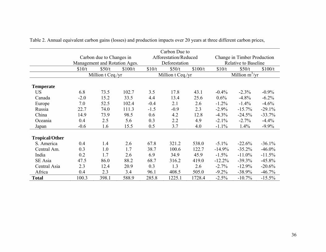
The short run production impacts of carbon policy are potentially substantial, and
they increase as the carbon price offered to the forestry sector rises. Table 2 presents
estimates of carbon sequestration and timber production from the global timber model in
Sohngen and Mendelsohn (2007). Carbon sequestration and reduced emissions from
management plus changes in rotation ages and from afforestation plus reduced
deforestation are shown for different regions of the world and different carbon prices.
Changes in timber production are also shown. All values are annual equivalent amounts
over the first 20 years period.
In the short-run (here defined as the first 20 years of the policy) output declines as
carbon sequestration occurs. These production impacts get steadily larger as carbon
prices rise. Globally, carbon sequestration and timber output are substitutes in the short-
run. Most carbon sequestered in temperate forests in the short run arises from changes in
management and changes in rotation ages. This contrasts with the tropics where most
carbon sequestration results from reductions in deforestation. Reductions in deforestation
also have strong production effects in the tropics because forestry outputs that are by-
products of the deforestation process are reduced. On average, in the temperate zone,
each 1 million t C increase in carbon sequestered reduces timber output by 0.3% on

27
average. In tropical zones, each 1 million t C increase in avoided emissions from
deforestation reduces timber output by 1.4% in the short-run.
5. EVALUATION OF CURRENT APPROACHES TO FORESTRY MODELING IN GLOBAL CGE ANALYSIS
While a number of partial equilibrium analyses of forestry and land use have
been developed to date (e.g., Murray et al., 2005; Sohngen and Mendelsohn, 2003;
Sathaye et al., 2006), few CGE models have fully incorporated land use, and none of
these have come to grips with forestry in a comprehensive fashion. The FARM model
described in Darwin et al. (1995, 1996) and Darwin (1999) is one example where land
use has been incorporated into CGE modeling, but the primary emphasis in that work was
on agricultural uses. One of the most important issues in modeling forestry is the
disaggregation of forest stocks by age class. This has a big impact on the potential for
carbon sequestration. The efficiency of forestry actions for sequestration is determined
by the rental value of carbon, but the value of carbon depends on future prices for timber
and carbon, as well as land rents for forestry. It has proven difficult thus far to account
for these dynamic stock effects when modeling forestry in a CGE context.
Despite the difficulty of incorporating forestry into CGE models, this book
highlights several important efforts in that direction. Hertel et al. (2007), for example,
incorporate reduced form marginal abatement cost functions derived from a partial
equilibrium model into the CGE framework. Their model is static, and considers only
near term abatement options. However, it is attractive in that it decomposes the total
sequestration response into the intensive (management and aging) and extensive margins,

28
as identified in Table 2. The problem with this comparative static analysis is that the
marginal abatement cost curves are dependent on the time horizon assumed. A longer
time horizon will generate flatter cost curves and hence different results. Operationalizing
this approach in a recursive dynamic CGE model would thus require that the authors shift
the abatement cost schedules over time.
Ahammed and Mi (2007) take a different approach using the GTEM model
(Global Trade and Environment Model). GTEM is a recursive dynamic CGE model.
Within the model, they explicitly account for the age class distribution of forests, and
shift forests from one age class to another over time. Their model does not "optimize"
harvest ages as would occur in a fully intertemporal model, but instead, they harvest a
fixed proportion of all age classes above 10 years old. Forestry competes with agriculture
uses of land via a constant elasticity of transformation (CET) function. And, if land shifts
into forests from agriculture, it shifts in during the youngest age class (i.e. new plantings).
If land shifts out of forestry, it shifts out proportionally from all age classes in the region.
So these authors begin to capture the differential carbon intensity of different age stands,
but they fail to capture the potential for changes in the optimal rotation length.
Golub et al. (2007) also utilize a recursive dynamic CGE model, however, they
take a different approach from Ahammed and Mi (2007). They focus on how the demand
for agricultural and forest products influences the allocation of land across different uses,
and how these demands affect decisions to access new land for agriculture and
commercial forestry. To capture the dynamics of forestry extraction, they link their
model with the dynamic optimization model of the forestry sector presented in Sohngen
and Mendelsohn (2007). The forestry model provides results on the value of extracting

29
timber resources over the period 2005 – 2025. Price changes for the forestry sector in the
recursive CGE model are then guided by prices from the forestry model. With technical
change in forestry processing sectors allowed to adjust to hit these price targets, the CGE
model is solved to determine forestry land use and output. Golub et al. (2007) focus on
changes in forest lands in the no-carbon price baseline, but their approach could be
adapted to the examination of a carbon policy by targeting the associated changes in land
rents over time. The strength of this approach is that it draws directly on the intertemporal
partial equilibrium model of Sohngen and Mendelsohn (2006). But this may also be
considered the main weakness, since the model does not incorporate the forestry sector’s
responses changing market conditions directly.
Sands and Kim (2007) utilize a recursive CGE model to analyze land use. They
account for the age class distribution of forests, but because of the difficulties associated
with solving the dynamic optimization problem within their modeling framework, they
simplify the problem by assuming that forests are harvested from fixed age class over
time. They utilize the underlying yield functions for forest production to determine
steady state rotation ages for forests with and without carbon incentives. They also
utilize these yield functions to determine the land rents for forestry. Land is converted
from one use to another depending on relative land rents in much the same way as the
other CGE studies, but using a supply function in which the elasticity of supply depends
on the inherent heterogeneity of yields within a watershed. This permits the authors to
capture the important impact of carbon policies on optimal rotations. However, in doing
so, it ignores the near term market impacts of climate policy (up to 50 years) which may
be quite different from the steady state adjustments, as has been shown above.

30
The studies in this book and suggest that the range of approaches for
incorporating forestry stocks into CGE models is fairly wide. Ahammad and Mi (2007)
and Sands and Kim (2007) take an approach that accounts for forestry stocks directly.
They have different methods for harvesting stocks, for example, Ahammad and Mi
(2007) harvest proportionally from different age classes (similar to approaches used in
static equilibrium modeling in the U.S., see Adams and Haynes, 1980 and Sohngen and
Sedjo, 1998). Alternatively, Sands and Kim (2007) harvest from a fixed age class, where
this age class is determined by static net present value calculations. Hertel et al. (2007)
take an indirect approach and incorporate marginal abatement cost functions from a
forestry sector model directly into their static CGE model to determine near-term
abatement strategies. Golub et al. (2007) focus on land allocation and access questions.
They calibrate their model based on forestry prices, deforestation rates and sensitivity of
management input to changes in forest land rents found in Sohngen and Mendelsohn
(2007). It is not clear that any one approach is "better" than the others. Rather, each set
of authors has focused on different aspects of the problem. Future research should be
aimed a merging some of these different approaches in order to permit CGE modelers to
better capture the role of forestry in climate change scenarios.
6. CONCLUSION
This chapter evaluates the optimal response of the forestry sector to changing
economic circumstances over time – particularly in the context of a carbon policy in
which the forestry sector receives rental payments for carbon sequestered. These
responses are then considered in light of current approaches to modeling the forestry

31
sector in CGE models with an eye to evaluating how well these capture the relevant range
of economic responses.
The chapter begins with a description of the forestry management problem and
shows the importance of age-class management in forestry. Age class management has
strong implications for carbon sequestration in forestry, allowing foresters to rapidly
obtain additional carbon at relatively low carbon prices. In contrast, afforestation efforts
may take many years to begin and because the forests take many years to grow, the bulk
of the carbon associated with afforestation occurs in future periods. So capturing the
broad outlines of this option is an important, but complex task for CGE models; some
compromises are inevitable.
Based on the analysis in this chapter, we find that, in longer-run studies (e.g., 50
years or more), modelers may focus on steady state adjustments in forestry and calculate
timber flows and carbon balances based on the rotation ages implied by these steady state
formulae. However, for those interested in shorter-run effects (e.g., 20 years), the age
class and production effects may be quite different than those implied by steady-state
relationships. Over this shorter time frame, we find that forest output is likely to be
sacrificed in order to boost forest carbon stocks. This is the opposite response to that
which is observed in the long run, over which higher carbon prices also boost steady-state
forest output.
In addition to age class adjustments, the paper also examines changes in other
types of management activities which influence the stocking density of the forest -- and
through that density also carbon stock and output flows. We estimate that other
management activities can provide around 20% of total carbon sequestered in the

32
temperate zone for a given price, and thus are important to consider. The paper presents
the methods used to incorporate management in the global timber model of Sohngen and
Mendelsohn (2007). CGE modelers could either incorporate this stocking density
parameter directly, or calibrate the elasticity of substitution between other inputs and
forest land to give an equivalent response in output per hectare of forest land (see Hertel
et al. and Golub et al., this volume).
In summary, the forest sector poses one of the most difficult challenges facing
CGE modelers interested in capturing the full range of potential responses to climate
change policy. Because the forests grow relatively slowly, the forest capital stock can
only be adjusted over a period of decades – as opposed to months or years in the case of
other sectors (e.g., wearing apparel, autos or wheat). This very slow adjustment means
that it is important to account for the age profile of the forest stock, which also adjusts
only slowly to a new policy environment. Keeping track of this age profile, and managing
the forest optimally, requires use of a long-run, forward-looking model. Yet such models
remain relatively rare in the large scale, global CGE modeling literature due to problems
of computation and sheer manageability. Until these models become routine, authors will
need to continue to make various compromises in their research. Which compromise is
least damaging will depend on the objective of the research being undertaken.

33
7. REFERENCES
Ahammed H. and R. Mi. 2007. Modeling land use changes and greenhouse gas emissions in GTEM. Chapter X in Economic Analysis of Land Use in Global Climate Change Policy. Edited by T. Hertel, S. Rose, and R. Tol. Routledge. Adams, D.M., R.J. Alig, B.A. McCarl, J.M. Callaway, and S.M. Winnett. 1999. “Minimum Cost Strategies for Sequestering Carbon in Forests.” Land Economics. 75:360-74. Darwin, R., Tsigas, M., Lewandrowski, J., Raneses, A. 1995. "World agriculture and climate change: economic adaptations." Agricultural Economic Report No. 703, US Department of Agriculture, Economic Research Service, U.S. Government Printing Office, Washington, DC. http:\\www.ers.usda.gov\publications\aer703\aer703.pdf. Darwin, R., Tsigas, M., Lewandrowski, J., Raneses, A., 1996. "Land use and cover in ecological economics." Ecological Economics. 17: 157–181. Darwin, R.F., 1999. "A FARMer’s view of the Richardian approach to measuring agricultural effects of climatic change." Climate Change 41(3-4): 371–411. Golub, A., T. Hertel, and B. Sohngen. 2007. "Modeling the Long Run Supply and Demand for Land." Chapter X in Economic Analysis of Land Use in Global Climate Change Policy. Edited by T. Hertel, S. Rose, and R. Tol. Routledge. Hertel, T., H-L Lee, S. Rose, and B. Sohngen. 2007. "Analysis of Global Land Use and the Potential for Greenhouse Gas Mitigation in Agriculture and Forestry. Chapter X in Economic Analysis of Land Use in Global Climate Change Policy. Edited by T. Hertel, S. Rose, and R. Tol. Routledge. Murray, B.C., B.L. Sohngen, A.J. Sommer, B.M. Depro, K.M. Jones, B.A. McCarl, D. Gillig, B. DeAngelo, and K. Andrasko. 2005. EPA-R-05-006. "Greenhouse Gas Mitigation Potential in U.S. Forestry and Agriculture." Washington, D.C: U.S. Environmental Protection Agency, Office of Atmospheric Programs. Richards, K.R., and C. Stokes. 2004. A Review of Forest Carbon Sequestration Cost Studies: A Dozen Years of Research. Climatic Change. 63: 1–48. Sands R. and M-K Kim. 2007. Modeling the Competition for Land: Methods and Application to Climate Policy. Chapter X in Economic Analysis of Land Use in Global Climate Change Policy. Edited by T. Hertel, S. Rose, and R. Tol. Routledge. Sathaye, J., W. Makundi, L. Dale, and P. Chan, and K. Andrasko. 2007. GHG Mitigation Potential, Costs and Benefits in Global Forests: A Dynamic Partial Equilibrium Approach. Energy Journal. 27: 127-162.

34
Sohngen, B. and R. Mendelsohn. 2003. “An Optimal Control Model of Forest Carbon Sequestration.” American Journal of Agricultural Economics. 85(2): 448-457. Sohngen, B. and R. Mendelsohn. 2007. "A Sensitivity Analysis of Carbon Sequestration." Chapter 19 in Human-Induced Climate Change: An Interdisciplinary Assessment. Edited by M. Schlesinger, et al. Cambridge: Cambridge University Press. Stavins, R. 1999. “The Costs of Carbon Sequestration: A Revealed Preference Approach.” American Economic Review. 89: 994-1009. Weyant, J.P, F.C. de la Chesnaye, G.J. Blanford. 2006. "Overview of EMF-21: Multigas Mitigation and Climate Policy." Energy Journal. 27: 1-32.
35
Table 1. Carbon intensity in temperate zone forests (t C/hectare), expressed relative to the baseline carbon intensity (1.0 = no change). By 2025 By 2055 $10/t $50/t $100/t $10/t $50/t $100/t
Proportional Change in t C/ha US 1.00 1.06 1.04 1.03 1.11 1.20 Canada 0.99 1.08 1.10 1.06 1.20 1.25 Europe 1.00 1.03 1.05 1.01 1.19 1.47 Russia 1.00 1.00 0.99 1.00 1.05 1.10 China 1.03 1.15 1.14 1.04 1.40 1.45 Oceania 1.00 1.00 1.00 1.00 1.00 1.01 Japan 0.98 0.98 1.16 1.01 1.03 1.14
36
Table 2. Annual equivalent carbon gains (losses) and production impacts over 20 years at three different carbon prices,
Carbon due to Changes in
Management and Rotation Ages.
Carbon Due to Afforestation/Reduced
Deforestation Change in Timber Production
Relative to Baseline $10/t $50/t $100/t $10/t $50/t $100/t $10/t $50/t $100/t Million t Ceq./yr Million t Ceq./yr Million m3/yr Temperate
US 6.8 73.5 102.7 3.5 17.8 43.1 -0.4% -2.3% -0.9% Canada -2.0 15.2 33.5 4.4 13.4 25.6 0.6% -4.8% -6.2% Europe 7.0 52.5 102.4 -0.4 2.1 2.6 -1.2% -1.4% -4.6% Russia 22.7 74.0 111.3 -1.5 -0.9 2.3 -2.9% -15.7% -29.1% China 14.9 73.9 98.5 0.6 4.2 12.8 -4.3% -24.5% -33.7% Oceania 0.4 2.5 5.6 0.3 2.2 4.9 -2.1% -2.7% -4.4% Japan -0.6 1.6 15.5 0.5 3.7 4.0 -1.1% 1.4% -9.9%
Tropical/Other
S. America 0.4 1.4 2.6 67.8 321.2 538.0 -5.1% -22.6% -36.1% Central Am. 0.3 1.0 1.7 38.7 100.6 122.7 -14.9% -35.2% -46.0% India 0.2 1.7 2.6 6.9 34.9 45.9 -1.5% -11.0% -11.5% SE Asia 47.5 86.0 88.2 68.7 316.2 419.0 -12.2% -39.3% -45.8% Central Asia 2.3 12.4 20.9 0.3 1.3 2.6 -2.7% -12.9% -20.6% Africa 0.4 2.3 3.4 96.1 408.5 505.0 -9.2% -38.9% -46.7%
Total 100.3 398.1 588.9 285.8 1225.1 1728.4 -2.5% -10.7% -15.5%

37
Figure 1. Proportion of carbon sequestration in temperate and tropical forests resulting from forestry actions for several different carbon prices over a 20 and 100 year period. All carbon is measured in annual equivalent amounts and the proportion of total storage is shown.
Temperate Zone (AEA, 20 yr, r=5%)
0.00
0.30
0.60
0.90
10 20 50 100
$/t C
Pro
porti
on Set-aside %Market %Mgmt %Age %Aff/Def %
Tropical (AEA, 20 yr, r=5%)
0.00
0.20
0.40
0.60
0.80
1.00
10 20 50 100
$/t C
Pro
porti
on
Mgmt %Age %Aff/Def %
Temperate Zone (AEA, 100 yr, r=5%)
0.00
0.30
0.60
0.90
10 20 50 100
$/t C
Prop
ortio
n Set-aside %Market %Mgmt %Age %Aff/Def %
Tropical (AEA, 100 yr, r=5%)
0.00
0.20
0.40
0.60
0.80
1.00
10 20 50 100
$/t C
Prop
ortio
n
Mgmt %Age %Aff/Def %
Note: All carbon gains are additional to the baseline. Set-aside % is the proportion of carbon due to setting aside forestland from timber production; Market % is the proportion of carbon stored in marketed productions; Mgmt % is the proportion due to improved management of timber stocks; Age % is the proportion due to increasing the rotation age of harvests; and Aff/Def % is the proportion due to land use change arising either from afforestation or reductions in deforestation.

38
Figure 2. Biomass and Merchantable timber yield functions for upland hardwoods in the U.S. south.
0
20
40
60
80
100
120
140
160
180
1 11 21 31 41 51 61 71 81 91Age
m3
per h
ecta
re
Biomass YieldMerchantable Yield

39
Figure 3. Growth rate and average annual flow of timber from upland hardwood type in the Southern U.S.
0
0.2
0.4
0.6
0.8
1
1.2
1.4
1.6
1.8
2
1 11 21 31 41 51 61 71 81 91Age
m3
per h
a pe
r yea
r
0
0.1
0.2
0.3
0.4
0.5
0.6
0.7
0.8
% A
nn. G
row
th R
ate
Avg Ann.FlowAnnual %Growth
Optimal rotation ageMaximum Sustainable
Yield

40
Figure 4. Present value of upland hardwoods in U.S. South under baseline (no carbon incentive) and three alternative carbon prices (derived from equation 5), assuming management inputs remain $56/hectare.
0
1000
2000
3000
4000
5000
6000
1 11 21 31 41 51 61 71 81 91
Age
NPV
($/h
a)
Pc=$200Pc=$100Pc=$50Pc=$0

41
Figure 5. Relationship between $/hectare management inputs, "n", and stocking density (delta, or δ).
0
100
200
300
400
500
600
0 0.5 1 1.5 2delta
Mgm
t Inp
uts
($/h
ecta
re) n=0.05
n=0.09n=0.13

42
Figure 6. Age class distribution of upland hardwood stands in the Southern U.S. in the baseline and climate mitigation scenario (high damage) from Sohngen and Mendelsohn (2006).
Initial
012345678
10 20 30 40 50 60Age
Mill
ion
Hec
tare
s
BaselineHigh Damage
Year 20
0
2
4
6
8
10
12
14
10 20 30 40 50 60Age
Mill
ion
Hec
tare
s
BaselineHigh Damage
Year 30
0
2
4
6
8
10
12
14
10 20 30 40 50 60Age
Mill
ion
Hec
tare
s
BaselineHigh Damage
Panel A: Initial Stock
Panel B: Year 20
Panel C: Year 30
43
Figure 7. Aboveground carbon stored in natural southern pine stands in the United States in the baseline and the high damage carbon mitigation scenario.
0
500
1000
1500
2000
2500
2005 2015 2025 2035 2045Year
Milli
on t
C a
bove
grou
nd
BaselineHigh Damage

44
Figure 8. Timber price index for baseline and high damage carbon policy scenario, derived from Sohngen and Mendelsohn (2007).
90
95
100
105
110
115
120
2005 2015 2025 2035 2045Year
Tim
ber P
rice
Inde
x (2
005
= 10
0)
BaselineHigh Damage

45
Figure 9. Annual timber harvests in southern upland hardwood stands in the United States in the baseline and the high damage carbon mitigation scenario. Estimates are taking from the midpoint of each decade, starting with 2010 to illustrate harvests during the 2005-2014 decade.
0
10
20
30
40
50
60
70
80
90
2010 2020 2030 2040 2050Year
Tim
ber H
arve
st (m
illio
n m
3/yr
)
BaselineHigh Damage