the parkes front-end controller and noise-adding radiometer · project require- ments and other ......
TRANSCRIPT

TDA ProgressReport42-102
N91-11983,-. ,,8
August15, 1990
The Parkes Front-End Controller and
Noise-Adding RadiometerT. J. Brunzie
Radio Frequency and Microwave SubsystemsSection
A new front-end controller (FEC) was installed on the 64-m antenna in Parkes,Australia, to support the 1989 Voyager 2 Neptune encounter. The FEC was added
to automate operation of the front-end microwave hardware as part of the Deep
Space Network's Parkes-Canberra Telemetry Array. Much of the front-end hard-
ware was refurbished and reimplemented from a front-end system installed in 1985
by the European Space Agency for the Uranus encounter; however, the FEC and its
associated noise-adding radiometer (NAR) were new JPL designs. Project require-ments and other factors led to the development of capabilities not found in standard
DSN controllers and radiometers. The Parkes FEC/NAR performed satisfactorily
throughout the Neptune encounter and was removed in October 1989.
I. Introduction
The 64-meter Parkes Antenna of the Australian Tele-
scope National Facility (or the Parkes antenna) was tem-
porarily used to enhance X-band (8.42 GHz) receiving ca-pability from the Voyager spacecraft during the Neptune
encounter in 1989. The Parkes antenna formed part of
the DSN Parkes-Canberra Telemetry Array (PCTA) andwas outfitted with DSN-compatible hardware, including a
microwave front end, telemetry receiver, data recorders,
and radio science equipment. Much of the hardware was
refurbished and reimplemented from the front-end sys-
tem developed by the European Space Agency (ESA)
for the Uranus encounter in 1986; however, the previ-
ous front-end monitor and control system was replaced
with a new JPL design. (For an overall description of
the design and installation of the front-end system, see
[1,2].) A block diagram of the front-end system is shownin Fig. 1.
The Parkes front-end controller (FEC) centralized and
automated the monitoring and control of the front-end sys-
tem, tying together equipment located in a NASA trailernext to the antenna with hardware located in the antenna's
aerial cabin. A block diagram of the FEC is shown in
Fig. 2.
The primary tasks performed by the FEC were to
(1) Monitor and control the antenna waveguide switches
and the polarizer drive assembly using a remote
switch/control unit and telltale monitoring.
119
https://ntrs.nasa.gov/search.jsp?R=19910002670 2018-08-21T17:08:16+00:00Z

(2) Measure system operating noise temperatures usingthe Y-factor technique through the automated wave-
guide switches, quartz thermometer, dual traveling-
wave maser (TWM) control assembly, and powermeter.
(3) Measure gain versus frequency of the TWMs, with
storage, retrieval, and display.
(4) Perform remote-controlled, noise-adding radiometerfunctions through automation of the noise diodes
and the RF detector power meter during antenna
calibration. Functions included returning a time-
varying analog signal, representing operating noisetemperature, and periodic calibration of the noisediodes.
(5) Chart performance history, provide status updates,and generate alarm messages for the closed-cycle
refrigerator/compressor monitor system [3].
(6) Monitor alarms for the downconverters, monitor re-ceiver, and test signal upconverter, including power
supplies, local oscillator power levels, timing, and
phase-lock conditions.
The overall functions and components of the Parkes
FEC are described in [1], which details the front-end sys-
tem design before it was implemented. This article will fo-cus primarily on the noise-adding radiometer (NAR) func-
tion of the FEC, since adding this capability comprised a
major design effort during FEC development.
Typically, NAils at DSN tracking stations are imple-
mented in the form of a precision power monitor (PPM)
assembly [4]. But in the case of the Parkes antenna, aPPM was not installed for the Neptune encounter because
of budgetary constraints. Instead, a new NAR design was
developed as part of the new Parkes front-end controller.
The NAR met all requirements (see Table 1) and func-tioned without difficulty during the Voyager Neptune en-
counter. The FEC/NAR equipment was removed from the
Parkes antenna on October 2, 1989 and returned to JPL.
II. NAR Requirements
As was mentioned, one of tile functions performed by
tile Parkes FEC was radiometric measurement of the oper-
ating noise temperature of the receiving systems. System
noise temperature data are needed for RF feed focusing,
collection of pointing data, and measurement of baseline
atmospheric effects. All radiometers determine noise tem-
perature by comparing receiver noise level against a cali-brated noise source. The radiometer most commonly used
in the DSN is referred to as a noise-adding radiometer be-
cause it periodically adds calibrated noise to the signal
during the measurement process [5].
Requirements for the Parkes NAR originated from the
need to calibrate the pointing and focus of the antenna af-
ter the new front-end package was installed. This type of
calibration is performed by pointing the antenna at extra-
galactic radio sources, quasi-stellar objects that radiate at
radio frequencies. The resulting increase in receiver noise
level caused by these radio sources appears as a rise in
noise temperature that is detected and measured by theradiometer. Optimum antenna focus and pointing calibra-
tion is achieved by varying equipment positions and other
parameters in the aerial cabin, RF package, and feedhorn
until a peak in system noise temperature is obtained.
During pointing calibration, the telescope makes two
orthogonal sweeps across the catalog coordinates of a star,
digitizing and recording the system temperature as a func-
tion of position. The antenna system computer derives aGaussian curve from each sweep, then mathematically con-
structs a model that fits these Gaussian curves to previ-
ously cataloged information on the flux and position of thestar. The difference between the cataloged values and the
center of the sweep is the pointing error. The procedure is
repeated for several combinations of azimuth and elevation
angles to model and systematically eliminate these point-
ing errors, tlowever, these pointing curves are distorted
somewhat by poor gain stability in the receiving systemand also by insufficient NAR sample resolution. The sta-
bility requirement for the Parkes NAR was 0.1 K during
the sampling time (corresponding to a gain stability of
0.02 dB) and the resolution requirement was 0.01 K forreturned samples.
Ideally, the computers that control the pointing and fo-
cusing of the Parkes antenna would receive a continuous,
instantaneous feedback of system temperature with infi-nite resolution. In practice, each measurement is limited
in resolution and requires some minimum amount of inte-
gration time before a suitable system temperature sample
can be produced. Tile Parkes NAR was required to return
samples at a rate of 10 per second or faster, with 20 sam-
ples per second desired. These temperature samples wereto be supplied as time-varying analog voltages sent to the
control room through coaxial cable.
Other constraints limited design options for the Parkes
NAR. Since radiometer sample resolution, sampling rate,system temperature, noise-diode selection, and system
hardware characteristics are not independent parameters,
they could not be designed as such. Attempts were made
120

to minimize conflicts in requirements through efficient soft-ware design, but some trade-off in performance was nec-
essary. Project requirements that limited the design in-
cluded the need to use existing PPM components to savetime and reduce cost and the need to time-share hardware
and software with other front-end functions.
III. FEC/NAR System Description
The Parkes tracking station (designated DSS 49) was
configured for the Voyager Neptune encounter as a two-
channel X-band receive-only system, using two cryogenic
maser amplifiers. The front-end package, which containedboth masers and the microwave feed, was positioned at the
prime feed focus in the antenna's aerial cabin. The NAR
noise-diode assemblies and support equipment were part
of the front-end package. The Voyager telemetry receiver
and associated signal-processing equipment were located
in a double-wide trailer just outside the antenna pedestal.The associated FEC equipment was divided between these
two locations (see Fig. 1) [2].
A. Front-End Controller
1. Description. The FEC consisted of a nmltibus
computer providing a card cage, power supply, and en-closure with slides. It monitored and controlled the mi-
crowave electronics in the antenna front end and provided
for two modes of radiometer operation: total-power and
noise-adding. A block diagram of the FEC is shown in
Fig. 2.
The FEC central processing unit (CPU) was aMultibus-based Intel 8086 single-board computer contain-
ing GP-IB and digital-to-analog (D/A) converter piggy-
back cards. FEC support boards included two ROMboards, a RAM board, a four-port serial communications
board, a 3- by 24-bit parallel communications board, and
a JPL-built pulse-train frequency counter board. Most of
the hardware interfaces for NAR operation used ports on
input/output (I/O) boards shared with other FEC func-
tions. The only additional hardware added to the FECfor NAR operation was the D/A converter card and the
pulse-train frequency counter board. Monitor and control
signals for the NAR shared the same communications net-
work used by other FEC functions.
The FEC D/A converter provided two analog signals
for NAR operation, the control signal for the RF power-
detector drawer (RF detector) internal attenuator and the
analog system temperature output. A channel on the par-allel I/O board provided 16 bits for the RF detector in-
put channel select and confirmation telltales as well as the
diode modulation drive output. Noise diode selection and
confirmation was performed via an IEEE-488 GP-IB in-terface to an HP 3488A switch/control unit located in theaerial cabin.
The pulse-train frequency counter board, a standard
PPM design, provided an integrate-and-dump means of
measuring the output frequency of the RF detector drawer
(which is a function of input power). Once instructed to
begin a measurement, the board operated unattended, in-
terrupting the CPU when data collection was completed.By counting input pulses and system clock ticks simulta-
neously, the board allowed the FEC to collect both timing
and RF power data. Dividing the number of input pulses
by measurement duration yielded average frequency, which
was then further processed to yield input power and sys-tem temperature, as will be discussed further in Section B.
2. Operation. The FEC was controlled through threeCRT terminals, each able to issue commands and receive
displays. The "local" terminal was located in one of thefront-end control racks in the trailer and was used for front-
end maintenance and testing. It also was used exclusively
for operation of the NAR during spacecraft tracking. Tile"remote" terminal was located ill the antenna control room
oil the third floor of the antenna pedestal and was used
by Parkes personnel to operate the NAR in support of
antenna calibration and X-band radio astronomy observa-tions. The "data ]ink" terminal was located in the control
room at the Canberra Deep Space Communications Cen-
ter (CDSCC) and was used to monitor front-end health
and status via modem during pre-encounter periods whenthe antenna was not being operated by station personnel.
All three of these terminals were able to send commands
and monitor fi'ont-end status at any time, but only one
terminal at a time fimctioned as the master terminal, pos-
sessing the ability to lock the front-end configuration for
security during actual tracking operations. The masterterminal was selected via a switch on the front of the FEC
chassis. All data, commands, and information graphics
could be printed on a local printer.
Radiometer data were made available by CRT displays,
printouts, and via a time-varying analog signal. The dis-
play information (which could be suppressed to prevent
interference with other FEC commands) was copied to
all three terminals for simultaneous display. Printouts
of these displays were made by connecting a printer tothe CRT. The analog output, available at the FEC back
panel, represented system temperature values as voltagelevels. This signal was updated with each temperature
sample computed, transmitted to the pedestal third floor
121

via coaxial cable, and used to drive a strip-chart recorder
and analog front end on the Parkes antenna computer forpointing calibration and radio science data collection.
3. Commands. Commands for the FEC were grouped
into menus according to function. Each menu item in-
cluded the command name, a brief functional description,
and a syntactic representation of parameter types. Syntax
and range checking was enforced; individual error messages
explained how to correct command errors. Each group hada menu and one or more corresponding status displays.
Most commands also responded to a "query," which pro-
duced a one-line status display for the associated function.
FEC menus and status displays that pertained to the ra-
diometer are shown in Figs. 4 through 9.
4. Interfaces. The FEC provided cabling inter-faces with the front-end equipment via IEEE 488, parallel-
transistor-transistor logic (TTL) control lines, RS-232serial communication lines, and 50-ohm coax. The equip-
meat interfaces are described in ill.
B. Noise.Adding Radiometer
It is difllcult to describe the NAR on a component level;
it can more readily be conceptualized as a function of the
FEC than as a set of components. Dedicated NAR com-
ponents included the noise diode assemblies (located on
the maser package in the aerial cabin), RF power-detector
drawer (located below the FEC in front-end control cabi-net no. 2), and its associated frequency-counter board (lo-
cated within the FEC). These components are described
below, along with NAR operation and calibration. A de-
scription of the NAR design before it was implemented is
detailed in [6]; however, several changes have been made tothis design since the report was published. Block diagrams
of the NAR are shown in Figs. 2 and 3.
1. Nolse-Diode Assemblies. Two noise-diode
assemblies were recovered from the ESA Parkes front-
end system, implemented during the Voyager Uranus en-
counter ill 1986. Each assembly consisted of an oven with
three diodes and a power supply. Each diode was capable
of three noise levels, depending on the value of its sup-ply current. The diode's power supply assembly contained
three independent current sources, one per diode. Any of
the three current levels could be selected through threerelay inputs and monitored with three relay telltales. A
separate TTL-level input for each diode provided instant
switching of the supply current, allowing rapid diode mod-ulation.
The relay inputs, telltales, and modulation-drive signalswere designed to be monitored and controlled by a PPM
through a PPM NAR controller assembly. But, in this
case, the PPM controller was functionally replaced by theFEC, which controlled the noise diodes with an HP 3488A
switch/control unit (SCU). This unit was a rack-mountedprogrammable device that used removable interface cardsto monitor and control various functions. Communication
with the SCU was provided by an IEEE-488 GP-IB stan-
dard bus that connected the FEC with equipment in thetrailer and the aerial cabin.
Two SCU bidirectional digital I/O interface cards were
used by the NAR to drive the noise diode power supply
relays and to sense the relay tell-tales. Each card pro-
vided sixteen channels programmed for eight bits input
and eight bits output. Although there are potentially nineinputs and nine outputs for each noise diode assembly,
only seven diode temperatures were standard on the units:
0.25, 0.5, 1, 2, 4, 8, and 50 K. Each card provided indepen-
dent closed-loop diode selection for one of the two maserchannels.
Because diode modulation requires precisely coordi-
nated switching that the SCU cannot provide when us-
ing a remote, shared GP-IB, tile SCU was not used forthis purpose. A single modulation signal was transmitted
separately from the trailer on a coaxial cable and used to
modulate all six diodes simultaneously. And because the
project requirements for the NAR were limited to pretrackcalibration support, no attempts were made to provide
the multiple-diode selection and independent modulation
schemes sometimes desired for radio science applications.
Noise output was injected through a waveguide cou-pler between the feedhorn/ambient load switches and the
maser input flanges. The maser input flange served as
the reference point for calculating system temperatures.
The actual power measurements were made at the PCTA
telemetry receiver input in the equipment trailer.
2. RF Power-Detector Assembly. The Parkes
NAR RF power-detector assembly was a borrowed PPM
8.4-GHz (X-band) prototype square-law detector [7]. Orig-
inally, as described in [6], plans were made to use digital
signal-processing techniques to develop an alternative to
the PPM detector (the digital power meter). This choice
was motivated by the poor linearity of the PPM device,which results in inaccurate measurements. Because of bud-
getary constraints, however, the RF power detector was
incorporated into the Parkes radiometer design instead.
In typical DSN use, the RF detector is part of a PPM
operated by a PPM NAR controller [4]. However, for
the Parkes implementation, the detector was operated by
122

the FEC. The name "square-law" refers to the square-law
diode used by the detector to measure input signal power:
the voltage developed across the diode is proportional
(ideally) to the total power in the signal. This voltageis translated into a TTL-level pulse train whose frequency
represents signal power; the pulse train forms the output of
the assembly. For the 1989 Voyager encounter, the pulse-train frequency was measured using a J PL-designed digital
frequency-counter board.
Although the input power-output frequency relation-
ship of the RF detector assemblies was intended to be lin-ear, in practice it more closely resembled a parabola than
a straight line. The Parkes NAR and the PPM employ dif-ferent software techniques to counteract this characteristic,both of which are discussed in the next section. Additional
methods of compensating for this and other front-end non-linear behaviors are described elsewhere [8].
The RF detector assemblies (Fig. 3) provide two inter-
faces for controlling power measurement: an input selectorswitch and an RF attenuator. The input selector switch is
a parallel TTL-controlled video switch used to select one of
up to eight signal channels for measurement. The voltage-controlled attenuator is needed to adjust the signal level
at the diode and set the desired baseline output frequency.Attenuation is minimized at -7 volts and increases ex-
ponentially as the control voltage approaches a limit of+1 volt.
The voltage-to-frequency units in the detectors were de-
signed to output a frequency of 100 ttz with the detectorswitched to an internal ambient termination. The maxi-
mum output frequency that could be obtained with theParkes unit was 13.7 kHz. As a result, the detector pro-
vided a dynamic range just exceeding the approximately
12.5 dB in input power experienced by the Parkes radiome-
ter during operation. (System temperatures ranged from azenith clear-weather value of 20 K to the antenna-ambient-
termination-plus-noise-diodes value of 360 K.) This char-acteristic allowed the detector to be operated without
changes in the internal attenuator setting, once the proper
operating point was determined and the attenuator set
accordingly. As discussed in the following section, thischaracteristic was crucial for maintaining a consistentcalibration baseline.
3. Operation and Calibration. Although theParkes radiometer is referred to as a noise-adding radiome-
ter, the term is somewhat misleading: it could be op-erated as either a noise-adding radiometer (NAR) or as
a total-power radiometer (TPR). In the TPR mode, the
system temperature was derived from measurements of to-
tal RF power in the downconverter band. Therefore, sys-
tem temperature was measured nonintrusively, but was
subject to system gain instabilities and required periodicrecalibration on the ambient load to maintain accuracy.
In the NAR mode, system temperature was derived by
Y-factoring power measurements made with the noise
diodes modulating on and off. This mode reduced sensi-
tivity to gain changes and provided better resolution when
using larger noise diodes, but telemetry was degraded dueto the noise injected into the system.
In the NAR mode, the operator could specify which
noise diode to modulate by entering its temperature as
a parameter. The FEC did not require an exact value;it would find tile closest available diode and inform the
operator of its choice. The FEC could also automaticallymonitor the system temperature and select a diode that
would not increase tile system noise temperature by more
than two percent.
In tile TPR mode, noise-power measurements were con-
verted into system temperature using the flmdamental re-
lationship P = GkTB. Tile GkB value, referred to in FEC
displays as the "system gain factor," varied with system
gain and had to be calibrated prior to using the TPR,and periodically thereafter. The FEC performed a sys-
tem gain factor calibration operation only for the maserchannel selected. The automated sequence of events in-
volved selecting tile antenna ambient termination as the
signal source for the receive chain, performing a powermeasurement with the RF detector, restoring the original
configuration, and then solving for the system gain factor.
Further system temperature calculations used this value
until it was recalibrated at the request of the operator.
Adding an optional numeric parameter to the commandallowed manual setting of the system gain factor value.
Use of the NAR mode also required a calibration opera-tion. Noise diode reference temperatures can only be mea-
sured in situ, and can vary in value as their environment
changes, so they generally are measured prior to each use.
The process of calibrating the entire noise diode set for theselected maser channel was automated using a calibration-
transfer technique. This was done by selecting the antenna
ambient load as the signal source, taking NAR Y-factor
data using the largest noise diode, computing diode tem-
perature from the data, selecting the feedhorn as the sig-nal source, and measuring the sky temperature using the
newly calibrated large diode. Once the sky temperaturehad been measured, each of the remaining diodes was se-
lected for calibration using the sky temperature as a ref-erence. Once all the diodes were calibrated, the original
receive-chain signal source was restored. Adding an op-
123

tional numeric parameter to the command allowed manual
setting of the temperature of the active noise diode.
An estimate of system linearity and NAR health could
be obtained with a command measuring the additive noise
temperature of a medium-power diode at two different sys-
tem noise temperature levels and comparing the results.Typically, the radiometer first measured the baseline-
feedhorn system temperature in the TPR mode and then
the temperature with the medium diode turned on. Sec-
ondly, the TPR measured system temperature using the
ambient load with the highest noise diode on and then withboth the highest diode and the medium diode on. The dif-
ferences between the two measurements at each operatingpoint yielded a derived medium-diode temperature. The
percent difference between the two derived values was re-
ported to the operator as a measure of system linearity(Fig. 10).
Measurement resolution for a NAR is a function of inte-
gration time, diode temperature, system temperature, and
noise bandwidth. For systems that are not gain-stable,
NAR resolution is also affected by diode modulation rate.
NARs are gain-insensitive only when individual measure-
ment periods are short enough that the system gain does
not change appreciably during sample integration. Forshort integrations, a pair of relative measurements elimi-
nates the effects of a changing baseline power level. Slow
diode modulation rates allow gain instability effects to ap-
pear and degrade resolution. High diode switching rates
cause the controller to spend most of its time on pro-
cessing overhead and very little time collecting data. Ineither case, measurement resolution decreases. A diode
switching rate command provided the ability to adjust the
diode modulation rate to obtain the best results (typically
10-15 Hz for Parkes and other DSN antenna systems).
In some cases, it was desirable to manually modulatetile noise diodes or set the RF power-detector attenuator
level. A manual command allowed the operators to force
the diodes to turn on or off, or to return automatic con-
trol to the FEC. Another command allowed the operator
to override the automatic adjustment of the internal at-tenuator and manually set an attenuation level.
An additional operating mode not normally accessed bythe operator affected operation of the RF power detector.
One of two methods of determining noise-power level with
the detector could be selected. The default mode, referred
to as the "linear" mode, used a second-order transfer func-
tion (based on original measurements of the equipment)
to create a linearized relationship over the entire detectoroperating range. This relationship was between the RF
power entering the assembly and the power reading com-puted by the driver routines. As a result, the location of
the operating point was not critical; the internal attenua-
tor was always automatically adjusted to center the range
of measurable temperatures within the dynamic range of
the detector, and then held constant until a change in sys-tem configuration was detected. This type of operation
was critical for TPR mode use because of the large tem-perature difference between the ambient load calibration
source and the feedhorn source. Without it, the internal
attenuator would have to be adjusted to prevent clippingor to maintain a constant operating point, either of which
would change calibration baselines and decrease accuracy.
The alternate RF detector operating mode, known asthe "DSN" mode, was simpler and patterned after themethod used by the DSN PPM NAR. This mode could
only be used in conjunction with NAR operation, as it
allowed the detector's internal attenuator setting to be al-tered, erasing any calibration baseline. The DSN mode
dynamically fit a first-order equation to the detector fre-
quency response, thereby restricting power measurements
to a small, nearly linear region of the response curve. This
was done by adjusting the internal attenuator to maintain
a fixed output frequency for the diode off state prior to
each measurement. Noise power was computed by dynami-cally fitting a first-order equation to the off measurement
frequency and the detector's internal ambient terminationrest frequency.
IV. Monitor and Control
Because the Parkes FEC was never required to be used
at a Deep Space Communications Complex (DSCC), its
command format and monitor displays were not required
to follow DSN CMC/LMC interface agreements and con-vention. Originally, the FEC was to be connected to the
PCTA; thus, to maintain compatibility, the FEC com-
mand structure and displays were designed to meet PCTA
conventions. When the decision was made not to imple-ment the PCTA controller link, the FEC became a stand-alone controller and was connected to the Canberra DSCCvia a modem and data link.
V. Performance
A. Discussion
Probably the most important performance statistic for
judging the quality of a radiometer is the degree to which it
can resolve changes in system operating noise temperature.Reporting radiometer performance is not, however, as sim-
ple as quoting a measured value of temperature resolution.
124

Resolving capability depends on several factors: sample in-
tegration time, noise-diode temperature and switching rate
(for NARs), the bandwidth of the detected signal, and thesystem temperature itself. As a result, radiometer perfor-
mance is better expressed as temperature resolution versus
integration time for a specified noise-diode temperature at
a normalized system temperature.
In order to collect the data needed for radiometer per-
formance analysis, it is necessary to fix some of the vari-ables mentioned above. One of them, the system noise
bandwidth, is usually fixed by the hardware. Another in-volves holding the operating temperature of the system
constant during data taking, preferably at as low a tem-
perature as possible. This is because resolution varies in-
versely with system temperature, and high system temper-
atures (such as those obtained when viewing the antennaambient termination) can mask the performance capabil-
ity of a sensitive radiometer. One solution is to switch theantenna front end to a cold load constructed from a wave-
guide termination immersed in a liquid nitrogen dewar.
(Liquid helium would, of course, be even better.)
For convenience, DSN radiometer performance tests are
usually conducted using a clear sky as a source with the
antenna held steady, preferably at zenith to minimize the
path length through the atmosphere. Under ideal atmo-
spheric conditions, the sky at X-band appears as a con-stant source radiating at approximately 8.5 K. tIowever,
because the atmosphere contributes to the system operat-
ing temperature, and it is not constant, the system tem-perature does not stay constant. The most significant con-
tributing factor at frequencies used by the DSN is water
vapor. Unfortunately, even a sky that appears clear maystill contain large, variable amounts of water vapor, mak-
ing this technique only suitable for short test runs at best.
To obtain a thorough picture of radiometer perfor-mance under a wide variety of operating conditions,
system temperature data need to be collected for several
integration times and, in the case of NARs, using a vari-
ety of noise diodes. Calculating the standard deviation of
each group of measurements yields resolution as a function
of integration time and diode. Reducing all the data and
plotting yields a family of curves that can be compared totheoretical curves.
Fortunately, the data collection process can be simpli-
fied. By operating the radiometer at the shortest integra-tion time of interest and taking a large number of samples,
it is possible to integrate groups of samples by hand to ob-tain data points corresponding to longer integration times.
Data sets can be normalized to any desired system tern-
perature, and performance with other noise diodes can be
inferred from comparison to theoretical curves.
In interpreting a plot of radiometer performance curves,
two things should be examined. The first, of course, is how
closely the measured values compare to the correspondingtheoretical curve. The second is not so obvious: the lo-
cation of the theoretical curve itself. This curve is not a
universal plot true of all radiometers; it is constructed forthe characteristics of that particular radiometer and the
conditions under which the data were gathered. It is en-
tirely possible for a radiometer whose performance curvelies well above its theoretical curve to outperform a second
system whose performance nearly equals theory.
B. Parkes NAR Performance Data
It is unfortunate that only minimal time was made
available for system performance testing after the final ver-sion of the Parkes NAR was delivered and installed on the
antenna. Immediately after encounter, the radiometer was
disassembled and returned to JPL along with the rest of
the X-band front-end equipment. As a result, inadequate
performance data were obtained.
However, the Parkes NAR was designed to be used for
spacecraft tracking as well as antenna-pointing calibration;consequently, the NAR was operated continuously while
the station tracked Voyager 2 throughout encounter week
to provide tile Voyager radio science investigators with
baseline system noise temperature data. Although this
type of data is not ideally suited for radiometer perfor-mance measurements, a method was found to derive from
it a single performance curve for the NAR. The develop-ment of this method and the final results are described
next.
During the Voyager encounter tracks, the Parkes NAR
was instructed to integrate samples for a period of one
second using the 0.25-K noise diode. The antenna drivecomputer, already configured to digitize the NAR analog
output to support antenna pointing calibration, was repro-grammed to receive the system temperature samples andrecord them to floppy disk throughout each track.
These data sets were recorded by the Parkes computer
as raw analog-to-digital (A/D) converter values, not as
operating system noise temperatures. Unfortunately, the
proper conversion factors were not available to reconstruct
the original system temperatures and the continuity of the
data was disrupted by gaps due to tracking update activ-ities. These factors necessitated additional steps in the
data analysis, but did not impact the accuracy of the final
125

results. The conditions under which the data were taken
were, however, significant: poor weather, a moving an-tenna, and the use of the smallest noise diode, which has
the greatest variance in its calibrated value. These factors
degraded the measured radiometer resolution, unfavorablybiasing the final performance statistics.
C. Parkes Data Reduction
The first step toward reducing the encounter radiomet-
ric data was the transformation of the A/D values backto the original system temperature values. Fortunately,
while the NAR was operating, the FEC was instructed to
display a system temperature sample every 15 sec on thethree control terminals. Because the "data link" terminal
at the Canberra complex (an IBM PC) was programmed
to log all terminal input/output in a large internal buffer,these system temperature values were captured, recorded
on disk, and made available along with the A/D convertervalues.
This NAR log data set provided the information neces-
sary for reconstructing the original noise temperature val-
ues computed by the Parkes NAR. (The data sets couldnot serve as a basis for NAR performance analysis because
14 out of every 15 samples had been lost; contiguous datawere needed.)
Of the three A/D and four NAR log data sets returned
to JPL on disk, only day-of-year (DOY) 238--the day fol-lowing Neptune closest approach--existed electronically inboth forms. It is this data set that forms the basis for the
performance figures reported in this article.
Because each A/D data set was produced from a se-
ries of linear transformations (assuming linear responsesfrom the associated hardware), the transformation back
to system temperature values was also a linear process:
T[ = mCi + b
where
(i= 1,2,3,4,...,n)
T" = transformed A/D converter sample i
(best estimate of the original NAR Ti)
Ci = A/D converter sample i
m, b = transformation parameters
The transformation parameters were determined bymodeling the A/D and NAR log data sets, then substi-
tuting the model parameters into the above equation and
solving. Under more ideal measurement conditions, the
models would be simply the means of the two data sets.
However, because the antenna was in motion during thetrack, the varying length of the signal path through the
atmosphere resulted in a constantly changing baseline sys-
tem temperature. This required that a more complicatedmodel be used.
In the simpler case, the system-temperature model con-sists of a constant term. Movement of the antenna in-
troduces a second, time-varying component that accounts
for the change in atmospheric signal path length. To sim-
plify calculations, a plane-parallel model of the atmospherewas used; the relative increase in path length compared to
zenith could then be expressed more simply as the secant
of the zenith angle. Zenith angle can be easily computed
for any time of day using the coordinates of the source,the antenna, and standard astronomical tables.
The resulting system temperature models are then
Ci= Cc + Cssec(¢i)
Ti = Tc + Tssec(_3i)
where
Ci, Ti = model values for each data set
Cc, Tc = model constant terms
Cs, Ts = model scaling factors for time-
varying term
¢i = antenna zenith angle at time i
Model parameters were determined for each set using the
least-squares method with the data values as the depen-
dent variable and the corresponding see(¢i)'s as the inde-pendent variable.
Figure l l depicts the NAR log data set for most of
DOY 238 and its corresponding model curve. Imperfec-
tions in the fit indicate other physical processes (primarilyweather) that could not be modeled, but do not signifi-
cantly affect the transformation of the A/D data set. Once
the models were constructed and the transformation pa-rameters generated, the entire A/D data set for DOY 238
was converted to system temperature values. Because a
necessary condition for reducing radiometric data to reso-
lution figures is that the set have a constant mean, anadditional manipulation was needed.
One method of normalizing the mean of the systemtemperatures would be to subtract the model value from
126

each data point and add a constant; however, this methodis not sufficient. The problem is that sample resolution is
a function of the system temperature, which not only re-
quires that the mean be normalized, but that the variancebe normalized as well.
The proper conversion equation can be determined by
starting with the equation expressing ideal noise-adding
radiometer resolution performance [5,6]:
aT- _ l+_n- n
where
CrT = theoretical best resolution
T = system temperature during measurement, K
TD = noise-diode temperature, K
t = sample integration time, sec
B = noise bandwidth as seen by RF powerdetector, Hz
A simplification can be made in this case, where T _ 25 K
and TD = 0.28 K.
Then T/To >> 1 and the above equation simplifies to
2T _
O'T - TD VZ_
For samples taken with a constant integration time, this
can also be expressed as
aT 2
T2 Tov_-- constant
This relationship provides the means for properly normali-
zing the mean and variance in the data set, provided anestimate of the true system temperature is known for every
sample:
(T'-m) • TN _ + TNT['- _
where
T[' = normalized system temperature sample i
T[ = transformed A/D converter sample i
/_i = mean or "true value" of T[ (from model)
Tlv = mean normalized system temperature
The mean at each point is estimated by modeling the
data using the same method described earlier for convert-
ing the A/D data. Figure 12 shows a half-hour segmentof A/D data that has been converted to its corresponding
system temperature values and plotted, together with itsmodeled mean and then after normalization to a temper-
ature of 20 K.
A total of 12 half-hour segments of data, each consisting
of approximately 1700 one-second integrations, were ana-
lyzed for DOY 238. Once each segment had been normal-ized to a consistent mean and variance, it was reduced to
seven resolution figures corresponding to integration times
of 1, 2, 5, 10, 20, 50, and 100 seconds. Determining resolu-tion for one-second integration times was straightforward,
requiring only the calculation of the standard deviationof each block of points. Resolution for other integration
times required additional manipulation of the data.
To obtain data for longer integration times, it was nec-
essary to average together contiguous groups of one-second
data points. This technique manually duplicates what theNAR does automatically when integrating for long peri-
ods. One consequence of doing so is that the resulting
block of data is proportionally smaller than tile original,which increases the variance in its calculated resolution.
Each of the half-hour data segments was expanded in
this manner six times to produce a total of seven blocks
of data. Next, the standard deviation of all seven blocks
was calculated for each segment. The resulting twelve val-ues associated with each integration time were then re-
duced statistically to generate the final performance re-
sults. These results, together with the theoretical curve,
are tabulated in Table 2 and plotted in Fig. 13.
Although the Parkes NAR performance curve in
Fig. 13 does not match the ideal peformance curve for
a NAR with equivalent characteristics, it should not be
expected to do so. The data from which this curve was de-rived were not well-suited for performance measurements,
having been taken during cloudy weather while the an-
tenna was in motion. These conditions will degrade mea-
sured resolution, biasing the performance figures. The ac-
tual performance of the Parkes NAR should lie somewherebetween the measured and ideal curves.
Vl. Summary
The Parkes front-end controller was designed as a cost-
effective means of providing a DSN interface for support
by the Parkes antenna during the Neptune encounter.
127

The FEC design maximized the use of existing front-endhardware, implemented in 1985 by ESA for the Uranus
encounter, by adding special features and capabilities.
In particular, a new noise-adding radiometer design was
added that departed frora standard DSN design.
Much of the design effort for the NAR focused on per-formance improvements and operational innovations ne-
cessitated by project requirements. The FEC/NAR per-formed without problems during the encounter and wasremoved from the Parkes antenna in October 1989.
Acknowledgments
The author would like to thank C. Stelzried for providing suggestions on NAR
functionality and operation. Many thanks also to J. Loreman and D. Trowbridgefor their support during development at JPL and to G. Baines and R. Jenkins for
their support during on-site installation and testing. L. Hileman contributed a first
draft coding of the FEC software.
References
[1] D. L. Trowbridge, J. R. Loreman, T. J. Brunzie, and B. Jenkins, "An 8.4-GHz
Dual Maser Front End for Parkes Reimplementation," TDA Progress Report42-93, vol. January-March 1988, Jet Propulsion Laboratory, Pasadena, Califor-
nia, pp. 214-228, May 15, 1988.
[2] D. L. Trowbridge, J. R. Loreman, T. J. Brunzie and R. Quinn, "An 8.4-GHzDual-Maser Front-End System for Parkes Reimplementation," TDA Progress Re-
port 42-100, vol. October-December 1989, Jet Propulsion Laboratory, Pasadena,California, pp. 301-319, February 15, 1990.
[3] L. Fowler and M. Britcliffe, "Traveling-Wave Maser Closed Cycle Refrigerator
Data Acquisition and Display System," TDA Progress Report 42-91, vol. July-September 1987, Jet Propulsion Laboratory, Pasadena, California, pp. 304-311,November 15, 1987.
[4] C. D. Bartok, "Analysis of DSN PPM Support During Voyager 2 Saturn En-
counter," TDA Progress Report 42-68, vol. October-December 1981, Jet Propul-sion Laboratory, Pasadena, California, pp. 139-150, February 15, 1982.
[5] P. D. Batelaan, R. M. Goldstein, and C. T. Stelzried, "A Noise-Adding Ra-
diometer for Use in the DSN," JPL Space Programs Summary 37-65, vol. 2, Jet
Propulsion Laboratory, Pasadena, California, pp. 66-69, September 30, 1970.
[6] T. J. Brunzie, "A Noise-Adding Radiometer for the Parkes Antenna," TDA
Progress Report 42-92, vol. October-December 1987, Jet Propulsion Laboratory,Pasadena, California, pp. 117-122, February 15, 1988.
[7] M. S. Reid, R. A. Gardner, and C. T. Stelzried, "The Development of a New
Broadband Square Law Detector," JPL Technical Report 32-1526, vol. XVI, Jet
Propulsion Laboratory, Pasadena, California, pp. 78-86, August 15, 1973.
[8] C. T. Stelzried, "Non-Linearity in Measurement Systems: Evaluation Method
and Application to Microwave Radiometers," TDA Progress Report 42-91,
vol. July-September 1987, Jet Propulsion Laboratory, Pasadena, California,pp. 57-66, November 15, 1987.
128

Table 1. Perkes radiometer specifications
Parameter Specification
General
Number of receiver channels supported
Signal sources (per receive channel)
Radiometer operating modes
Nominal system noise temperature range
RF detector
Detector dynamic range
Nominal input noise power level
Input frequency bandwidthInternal attenuator control
Internal attenuator rangeDetector operating modes
Noise diodes
Diode selection control
Automatic diode selection criteria
Nominal diode temperaturesDiode modulation control
User-specifiable modulation frequency range
Sampling
Sampling criteria
User-specifiable sample integration time range
User-specifiable sample resolution range
Sample outputMeasurement modes
Sample output modes
User-specifiable sample display interval
Samples used in resolution calculation
Analog output
Ouput voltage range
Output resolutionUser-specifiable zero-volt noise temperature
User-specifiable noise temperature/voltage ratio
Calibration
Total power radiometer mode
Noise-adding radiometer mode
Linearity measurement points
Two, switchable
Antenna feedhorn;aerial cabin ambient
termination
Total power;
noise-adding
15 to 400 K
13.5 dB
-45 dBm
65 MItz
Manual or automatic0 to 50 dB
Dynamic first-order fit over
subrange of detector response;static second-order fit over
entire range of detector response
Manual or automatic
<0.1 dB added noise
0.25,0.5,1,2,4,8,50,(50+8) KManual or automatic
0.01 to 100 Hz
Integration time;sample resolution0.01 to 100 seconds
0.001 to 10 K/sample
Manual single-sample;
continuous in background
Display and analog output;
analog output only
1 to 15 seconds/sampleNone or 2 to 100
-5 to +5 volts
2.4 mV (12-bits)0 to 500 K
0.001 to 100 K/V
System gain factor
Noise-diode temperatures
Feedliorn/feedhorn+ 50 K;
ambient/ambient +50 K;
feedtlorn/ambient +50 K
129
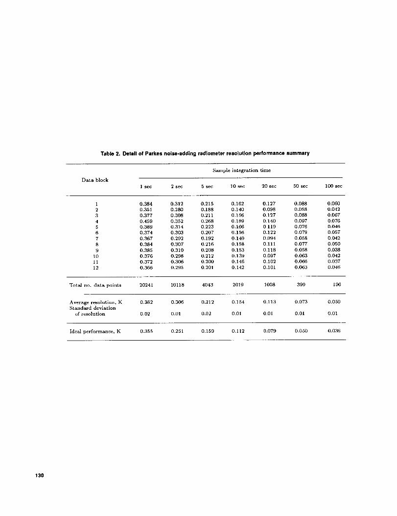
Table2.DetailofParkesnoise-addingradiometerresolutionperformancesummary
Data block
Sample integration time
1 sec 2 sec 5 sec 10 sec 20 sec 50 sec 100 sec
1 0.384 0.312 0.215 0.162 0.127 0.088 0.060
2 0.351 O. 280 0.188 O. 140 0.098 0.058 0.042
3 0.377 0.308 0.211 0.156 0.127 0.088 0.067
4 0.459 0.352 0.268 0.189 0.140 0.097 0.0765 0.389 0.314 0.223 0.166 0.119 0.076 0.046
6 0.374 0.303 0.207 0.156 0.122 0.079 0.057
7 0.367 0.292 0.192 0.140 0.094 0.058 0.042
8 0.384 0.307 0.216 0.158 0.111 0.077 0.050
9 0.385 0.310 0.208 0.153 0.118 0.058 0.038
10 0.376 0.298 0.212 0.139 0.097 0.063 0.042
11 0.372 0.306 0.200 0.146 0.102 0.066 0.037
12 0.366 0.295 0.201 0.142 0.101 0.063 0.046
Total no. data points 20241 10118 4043 2019 1008 399 196
Average resolution, K 0.382 0.306 0.212 0.154 0.113 0.073 0.050Standard deviation
of resolution 0.02 0.01 0.02 0.01 0.01 0.01 0.01
Ideal performance, K 0.355 0.251 0.159 0.112 0.079 0.050 0.036
130

X-BANDFEEDHORN I
AND POLARIZERASSEMBLY
1 _8400-8465 MHz
AMBIENT LOAD/FEEDHORN SELECT rAERtALCABIN _ ............. r _ .... / HPSWlTCH
AMBIENT I 1%',2;,_u%%_I / CONTROL
ITERMINATIONS _ ....
RADIOMETER I I I Ill
CALIBRATION t t DtODE I ISOURCE . . , r _'_ SELECT I I
DUAL_I'_S"_'_O_YI"--INO,_!O_EI'-- _ IAMPLIFIERS I I AND OVEN I_ I '"'_%_,_ I_
, _1"_1 ASSEMBLIES_t_[ _____ _'_ IDIODE I GP-IB I
I DUA_L_X:_ANU I MODULATION I BUS II _o.°v°E.?aRSI OR,VE I I
PARKES ANTENNA _ I I
r
VOYAGER2 / I PCTA I_ I ......... I I I-I=_n_T_rTn_ I TRAIN I FRO_N_T:EN_D_ I I ANALOG
TBEALSEBAN_YI_ I _;_;# I I i I"kEs_K?_----_1CgNE-".O.LL-E.U I--_TSYSMTpEEMRATURE
Fig. 1. Parkes front end (radiometer emphasized).
131

PARKESANTENNAPEDESTAL PARKES
ANTENNA DRWECOMPUTER
'REMOTE'TERMINAL
I I
CDSCC CONTROL ROOM
'DATA LINK'TERMINAL
I I
'LOCAL' ITERMINAL
I
CCR/
COMPRESSORMONITOR
ASSEMBLY
R_232SERIALI/O
BOARD
m
ANALOGOUTPUT
CARD
I8086 CPU
BOARD
IGP-IB
CONTROLLERCARD
PULSE-TRAINFREQUENCY
COUNTER BOARD
PARALLELDIGITAL
I/O BOARD
I
_
RF DETECTORATTENUATIONCONTROL
GP-IB EQUIPMENTIN TRAILER ANDAERIAL CABIN
RF DETECTORPULSE TRAIN
RF DETECTOR,_ INPUT SELECT
CONTROL
NOISE DIODEMODULATIONDRIVE
MASER INTERFACEPANEL MONITORAND CONTROL
Fig. 2. Parkes front-end controller assembly.
132

DOWNCONVERTER OUTPUT(300-365 M Hz)
CHANNEL1
CHANNEL2
AMBIENT ITERMINATION
INPUT SELECTOR
VIDEO SWITCH J
INPUT CHANNELSELECT ANDRELAY TELLTALES
PARALLEL IDIGITAL
I/O BOARD
VOLTAGE-CONTROLLEDATTENUATOR
ATTENUATORCONTROLVO LTAGE
ANALOG JOUTPUT
CARD
SQUARE-LAWDIODE POWER
DETECTOR
8086 CPUBOARD
I
RF POWER-DETECTOR ASSEMBLY
VOLTAGE-TO-FREQUENCYCONVERTER
TTL PULSETRAIN OUTPUT
I PULSE-TRAINFREQUENCY
COUNTER BOARD
II J
FRONT-END CONTROLLER ASSEMBLY
Fig. 3. Parkea radiometer RF power detector.
PFEC>help m
PFEC Front End Controller Measurement Help...The format for user input is: COMMAND PARAMETER
Cmnd Description
YFAC Perform Y-factor Measurement.
GAIN Compute Maser Gain Profile.
PMTR Operate Power Meter.
CCRH Chart CCR Performance History.
SYST Measure System Temperature (NAR).
NRES Set NAR Sample Resolution.
NRAT Set NAR Sample Rate.
DRAT Set NAR Diode Switching Rate.
NSAM Set Number of Resolution Samples.
CALG Calibrate System Gain Factor.
CALD Calibrate Noise Diodes.
DLTA Measure System Linearity Delta.
PFEC>
Parameter
[]],[2] [L]eft,[R]ight
[1],[z][M]easure,[C]alibrate
[I],[2] [MMddHHmm] [MMddHHmm]
[],[OFF],[C]ont,[D]isp [n] sec
[n] Kelvins
In]HzIn] Hz (Debug only)
[n][],[n] nW/Kelvin (CFG only)
[ALL],[n] Kelvins (CFG only)
[S]ky,[A]mbient,[F]ull Range
Fig. 4. Parkes FEC/NAR measurement help menu.
133

PFEC>help n
PFEC Front End Controller NAR Help...The format for user input is: COMMAND PARAMETER
Cmnd Description
PNAR Set Parkes NAR Command Mode.
NRCV Set NAR Input Source.NMOD Set total Power or Noise-Adding Mode.DMOD Set Square-Law Detector Operating Mode.DIOD Set NAR Diode Temperature.DACZ Set NAR D/A Zero-Volt Temperature.DACG Set NAR D/A Temperature Gain.NOIS Turn Noise Diodes On or Off.
NATN Set RF Assy Internal Attenuator.TMAS Set Maser Input Noise Temperature.TFOL Set System Follow-up Noise Temperature.GINS Set Maser Gain Instability.
PFEC>
Parameter
[OFF],[CFG],[OPR][]],[2],[TRM][TPR],[NAR][LIN],[DSN] (Debug)[A]uto,[OFF],[n] Kelvins (NAR)[A]uto,[n] Kelvins[A]uto,[n] Kelvins/Volt[A]uto,[OFF],[ON] (Debug)[A]uto,[n] Volts (Debug)[]],[2] [n] Kelvins[]],[2],[M]onRcvr [n] Kelvins[S]hort-term [n] dB,
[L]ong-term [n] dB/hr
Fig. 5. Radiometer configuration help menu.
PFEC>stat c
PFEC Configuration Status (237 07:32:14) Configuration is UNLOCKED
53.36K/MOD---+ 8100 MHz +....NARI I I
Horn/RCP ..........+....Maser ]....+.........+.......X........RF ]
8425 MHz/WB/PM ....+...............+ +.......X........Mon RcvrI I
Ambient Load......+....Maser 2....+.........+.......X........RF 2I I
ND OFF/OFF---+ 8100 MHz
Local CRT has command locking privileges.
PFEC>
Fig. 6. Front-end configuration status display.
134
PFEC>stat m
PFEC Temperature Measurement Status
System Temperature
Measurement Resolution
Ambient Load Temperature :
System Gain Factor
Gain Factor Age
Maser Input Noise Temp
System Follow-up Noise Temp :
Short-Term Gain Instability :
Long- Term Gain Instability :
TPR Resolution Uncertainty :
PFEC>
(236 13:27:54)
RF Ch ] RF Ch 2
15.328 15.037
0.025 0.02]
297.860 300.I63
12.823 8,983
00:02:38 00:13:25
4.05 3.92
0.13 0.29
0.03 0.03
0,]0 0.10
0.013 0,283
Kelvins
Kelvins
Kelvins
nW/Kelvin
Kelvins
Kelvins
dB
dB/hr
Kelvins
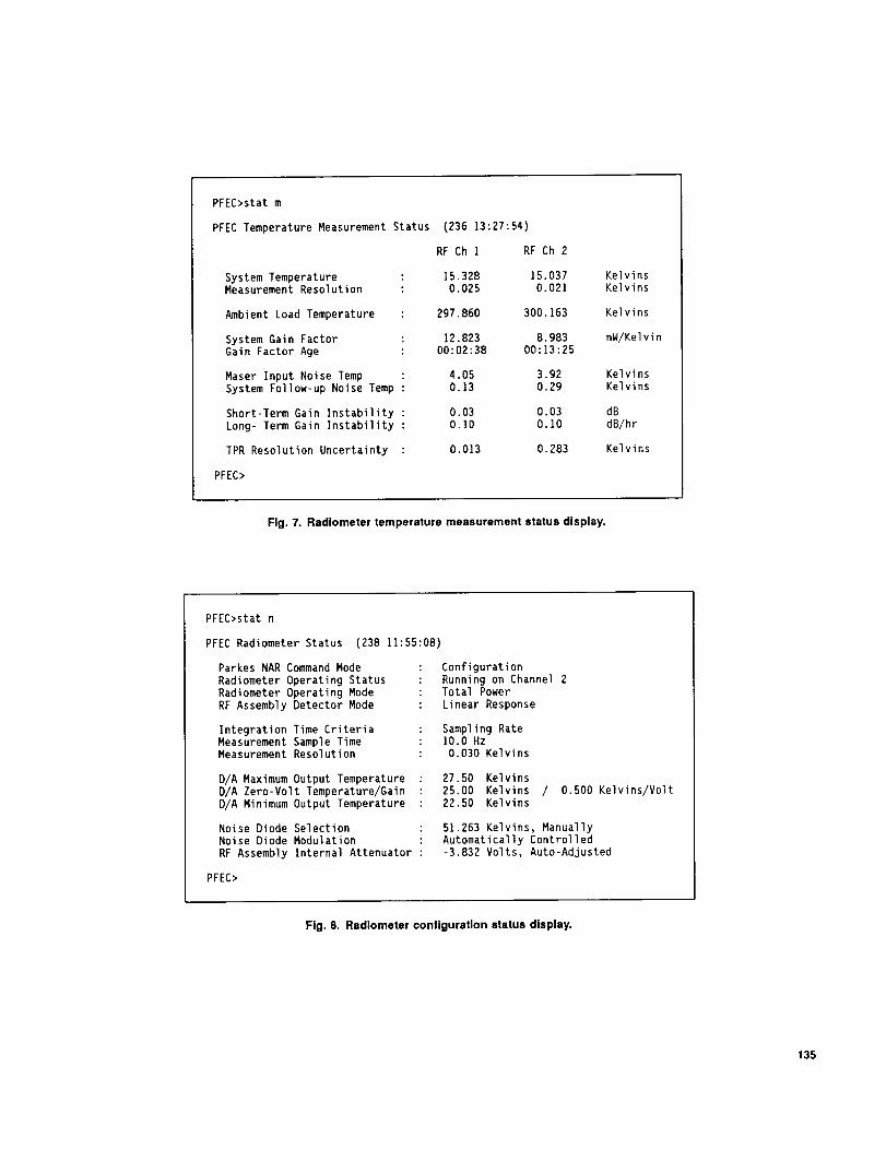
Fig. 7. Radiometer temperature measurement status display.
PFEC>stat n
PFEC Radiometer Status (238 11:55:08)
Parkes NAR Command Mode
Radiometer Operating Status
Radiometer Operating Mode
RF Assembly Detector Mode
: Configuration
: Running on Channel 2
: Total Power
: Linear Response
Integration Time Criteria : Sampling Rate
Measurement Sample Time : 10.0 HzMeasurement Resolution : 0,030 Kelvins
D/A Maximum Output Temperature : 27.50 Kelvins
D/A Zero-Volt Temperature/Gain : 25.00 Kelvins
D/A Minimum Output Temperature : 22.50 Kelvins
/ 0.500 Kelvins/Volt
Noise Diode Selection
Noise Diode Modulation
RF Assembly Internal Attenuator
: 51.263 Kelvins, Manually
: Automatically Controlled
: -3.832 Volts, Auto-Adjusted
PFEC>
Fig. 8. Radiometer configuration status display.
135

PFEC>stat d
PFEC Noise Diode Status (241
Noise Diode Temperatures
Noise Diode Calibration
PFEC>
12:17:31)
RF Ch ] RF Ch 2
: 0.223 0.250 Kelvins
: 0.483 0.500 Kelvins
: 1.183 1.000 Kelvins
: 2.089 2.000 Kelvins
: 3.938 4.000 Kelvins
: 9.032 8.000 Kelvins
: 52.382 50.000 Kelvins
: 61.414 58.000 Kelvins
: Calibrated Not Cal'd
Fig. 9. Noise diode status display.
T2 + 50K +8K
T2 + 50K
A Top HIGH
DELTA % = I'_T°p HIGH -ATop LOWIA Top LOW
P1
P1+ P8K
MASER INPUT POWER LEVEL
P2 + PSOK
P2 + PSOK+ P8K
Fig. 10. Parkes radiometer "Delta" command.
136

v
)-<
¢,9
3O
28
26
24
22-
20
I I I I
DATA RECORDED DURING VOYAGER 2 TRACK26 AUGUST, 1989 (DOY 238), 08:30 TO t5:00 UT
NOISE DIODE TEMPERATURE = 0.28 KINTEGRATION TIME = 1.0 sec/sample
L 1 L [08:15:00 09:39:00 11:03:00 12:27:00 13:51:00
UNIVERSAL TIME
Fig. 11. Logged NAR data and corresponding system noise temperalure model.
15:15:00
28
26
rr"24
F-<
22
20
18
I I I I
DATA RECORDED DURING VOYAGER 2 TRACK
26 AUGUST, 1989 (DOY 238), 08:29 TO 09:01 UT
NOISE DIODE TEMPERATURE = 0.28 K
_ INTEGRATION TIME = 1.0 sec/sample
NOISE TEMPERATURE
I ] I I08:28:00 08:34:48 08:41:36 08:48:24 08:55:12 09:02:00
UNIVERSAL TIME
Fig. 12. Transformed/)JD data, model, and normalized system noise temperatures.
137

v
z"O
=,O_3
10 0
6
4
2
10-1
6
4
2
10-2
10 0
, , i ' i ' ' ' '
DATA RECORDED DURING VOYAGER 2 TRACK
26 AUGUST, 1989 (DOY 238), 08:30 TO 15:00 UT
MEASOR,DEAL
PERFORMANCE _
NORMALIZED SYSTEM NOISE TEMPERATURE = 20 KNOISE DIODE TEMPERATURE = 0.28 KSYSTEM NOISE BANDWIDTH = 65 MHz
I I I I I I I I I
2 4 6 101 2 4 6 10 2
INTEGRATION TIME, sec
Fig. 13. Parkes noise-adding radiometer resolution performance
summary.
138