1

The long-run determinants of inequality:

What can we learn from top income data?∗

Jesper Roine†, Jonas Vlachos‡ and Daniel Waldenström♣

March 25, 2009

Abstract

This paper studies determinants of income inequality using a newly assem-bled panel of 16 countries over the entire twentieth century. We focus on three groups of income earners: the rich (P99-100), the upper middle class (P90-99), and the rest of the population (P0-90). The results show that peri-ods of high economic growth disproportionately increases the top percen-tile income share at the expense of the rest of the top decile. Financial de-velopment is also pro-rich and the outbreak of banking crises is associated with reduced income shares of the rich. Trade openness has no clear distri-butional impact (if anything openness reduces top shares). Government spending, however, is negative for the upper middle class and positive for the nine lowest deciles but does not seem to affect the rich. Finally, tax progressivity reduces top income shares and when accounting for real dy-namic effects the impact can be important over time.

Keywords: Top incomes, income inequality, financial development, trade openness, government spending, taxation, economic development JEL: D31, F10, G10, H20, N30

∗ We would like to thank three anonymous referees, Tony Atkinson, Thorsten Beck, Robert Gordon, Henrik Jordahl, Thomas Piketty, Kristian Rydqvist and seminar participants at Université Libre de Bruxelles, 3rd BETA workshop in Strasbourg, 2007 ETSG in Athens and 4th DG ECFIN Research Conference in Brussels 2007 for useful comments. Thanks also to Michael Clemens and Jakob Madsen for kindly sharing their data with us. Financial support from the Jan Wallander and Tom Hedelius Foundation and the Gustaf Douglas Research Program on entrepreneurship at IFN is gratefully ac-knowledged. † SITE, Stockholm School of Economics, P.O. Box 6501, SE-11383 Stockholm, Ph: +46-8-7369682, jesper.roine@hhs.se ‡ Department of Economics, CEPR & IFN, Stockholm University, SE-10691 Stockholm. Ph: +46-8-163046, jonas.vlachos@ne.su.se. ♣ Research Institute of Industrial Economics (IFN), P.O. Box 55665, SE-10215 Stockholm, Ph: +46-8-6654531, danielw@ifn.se.

2

1 Introduction

The relationship between inequality and development is central in the study of eco-

nomics. From fundamental issues about whether markets forces have an innate ten-

dency to increase or decrease differences in economic outcomes, to much debated

questions about the effects of “globalization”, distributional concerns are always pre-

sent: Does economic growth really benefit everyone equally or does it come at the

price of increased inequality? Is the effect perhaps different over the path of develop-

ment? Is it the case that increased openness benefits everyone equally, is it perhaps

especially the poor that gain, or is it the case that it strengthens the position only of

those who can take full advantage of increased international trade? Does financial de-

velopment really increase the opportunities for previously credit constrained individu-

als or does it only create increased opportunities for the already rich? What is the role

of government in all this? Theoretically such questions are difficult to resolve as there

are plausible models suggesting equalizing effects from these developments, as well

as models suggesting the opposite.1 Empirically problems often arise because these

effects should be evaluated over long periods of time and data is typically only avail-

able for relatively short periods.

This paper empirically examines the long-run associations between income inequality

and economic growth, financial development, trade openness, top marginal tax rates,

and the size of government.2 While these variables are not direct measures of typically

suggested causes of changes in income distribution, such as globalization, technologi-

cal change or social norms, studying their relation to inequality over time seems as an

important step toward understanding such broader concepts. The main novelties of

our study lie in the uniquely long time period for which we have data and in the focus 1 Just to give some examples: one may distinguish between theories that predict markets to be innately equalizing, disequalizing or both (depending on initial conditions). Mookherjee and Ray (2006) give a useful overview of the literature on development and endogenous inequality based on such a division. Winters et al. (2004) give an overview of evidence on the relation between trade and inequality, Cline (1997) summarizes different theoretical effects of trade on income distribution, while Claessens and Perotti (2005) provide references for the links between finance and inequality, presenting theories which suggest both equalizing effects as well as the opposite. We will discuss some of the suggested mechanisms in more detail in Section 2 below. 2 As our focus is on pre-tax income we do not explicitly address questions of redistributive policy but rather the effects of taxes and government size on income before taxes and transfers. See Bardhan, Bowles and Wallerstein (eds.), 2006, for several contributions on the relation between various facets of globalization and their impact on the possibilities to redistribute income).

3

on top income shares. We use the newly compiled Atkinson-Piketty dataset for 16

countries over the whole of the twentieth century (see Atkinson and Piketty, 2007,

2009).3 While previous studies have only had comparable data from the 1960s (at

best), our series begin at the end of the “first wave” of globalization (1870–1913),

continues over the interwar de-globalization era (1913–1950), the postwar “golden

age” (1950–1973) and ends with the current “second wave” of globalization.4 Hence,

in contrast to relying on shorter periods of broader cross-country evidence, our dataset

allows us to study how inequality has changed over a full wave of shifts in openness

as well as several major developments in the financial sector. In terms of the role of

government, our long period of analysis implies that we basically cover the entire ex-

pansion of the public sector and the same is true for the role of income taxation, which

was non-existent or negligible at the beginning of the twentieth century.5

The focus on top incomes, and on concentration within the top, means that we can ad-

dress a special subset of questions regarding the extent to which economic develop-

ment is particularly pro-rich.6 More precisely, our data allows us to distinguish be-

tween the effects on, broadly speaking, the “rich” (top executives and individuals with

important shares of capital income), the “upper middle class” (high income wage

earners), and the rest of the population.7 As has frequently been pointed out in the re-

cent top income literature the top decile is a very heterogeneous group. The lower 3 Even though the choice of countries - mostly developed economies - is mainly a result of data avail-ability it has some positive side effects. We are, for example, able to trace a fixed set of relatively simi-lar countries as they develop rather than letting different countries represent stages of development. Having similar countries is also important especially when thinking about theoretical predictions from openness which are often diametrically different for countries with different factor endowments, tech-nology levels etc. Parallel to our work, Andrews, Jencks, and Leigh (2008) also use the new top income inequality data to study the relation between inequality and growth, while we focus on determinants of inequality. 4 These periods are quoted in, for example, O’Rourke and Williamson (2000), O’Rourke (2001), and Bourguignon and Morrison (2002). These studies discuss various aspects of globalization and inequal-ity over these early periods but they did not have sufficient data to analyze developments in detail. Also see Cornia (2003) for a discussion of differences in within-country inequality between the first and second globalization. 5 In fact, the introduction of a modern tax system is typically what limits the availability of data on in-come concentration. 6 Examples include, models of how aspects of these developments creates extreme returns to “super-stars”, or models of capitalists and workers where capitalists benefit disproportionately would, when taken to the data, translate to isolated effects for a small group in the top of the income distribution. 7 Clearly, any such division is arbitrary but the results are not sensitive to variations in the definitions of these top groups, e.g., by choosing to look at the top 0.5 percent instead of the top percentile as “the rich”. Furthermore, data on the composition of incomes indicate clearly that the top percent as a whole is very different from the rest of the top decile, especially with regard to capital income shares (we dis-cuss this in section 3). A similar classification, but with respect to wealth, is made in Hoffman, Postel-Vinay and Rosenthal (2007).

4

parts of it typically consists of employed wage earners with relatively stable income

shares, while the top has a different composition of income with larger capital shares

and with much larger fluctuations over time.8 Examining whether some development

affects everyone in the top of the distribution in similar ways, or if there are clear dif-

ferences within the top, holds important keys to what is driving developments of ine-

quality.

Our empirical analysis exploits the variation within countries to examine how changes

in top income shares are related to changes in economic development, financial devel-

opment, trade openness, government expenditure, and taxation.9 Using a panel data

approach allows us to take all unobservable time-invariant factors, as well as country

specific trends into account. We also allow the effects to differ depending on the level

of economic development, between Anglo-Saxon countries and others, and between

bank- and market-oriented financial systems.10

Several findings come out of the analysis. First, we find that periods of high economic

growth are strongly pro-rich. In periods when a country’s GDP per capita growth has

been above average, the income share of the top percentile has also increased. By con-

trast, the next nine percentiles (P90-99) seem to loose out in these same periods. As

we find this relation to be similar at different stages of economic development, it

could indicate that recent findings of high productivity growth mainly benefiting the

rich in the U.S. postwar era (Dew-Becker and Gordon, 2005, 2007), is a more general

phenomenon across both countries and time. This result is in line with top incomes

being more responsive to growth (e.g., through compensation being related to profits).

8 For evidence on much of changes in top income concentration stemming from the very top, see At-kinson and Piketty (2007, 2009). 9 We will discuss our empirical strategy in more detail below, but it is important to note, right from the outset, the distinction between our first difference approach and correlations in levels. For example, our result that periods of high growth increases the income share of the rich disproportionately does not imply a positive correlation between growth and top income shares. Indeed a key observation, made in e.g., Piketty (2005) and Piketty and Saez (2006), is that when inequality was at its highest, in the be-ginning of the Twentieth Century, growth was relatively modest, compared to the post-war period when growth was high and inequality levels low. 10 As we will discuss in more detail below, these are some of the dimensions in which we may expect differences in development of inequality either on theoretical ground or based on previous empirical findings.

5

Furthermore, we find that financial development, measured as the relative share of the

banking and stock market sectors in the economy, also seems to increase the income

share of the top percentile. That these effects are causal is supported by our finding

that banking crises a have a strong negative impact on the income shares of the rich

(while this is not the case for currency crises). When interacted with the level of eco-

nomic development it turns out that the result is mostly driven from a strong effect in

the early stages of development. This result is in line with the model suggested by

Greenwood and Jovanovic (1990) where financial markets initially benefit only the

rich but as income levels increase (and with them the development of financial mar-

kets) the gains spread down through the distribution.11 It is also of particular interest

since a recent study by Beck, Demirguc-Kunt and Levine (2007) finds that financial

development disproportionately benefits the poor.12

Our results with respect to the role of government indicate that government spending

as share of GDP has no clear effect on the incomes of the top percentile, but seem to

be negative for the upper middle class and positive for the rest of the population.

Higher marginal taxes, however, have a robustly negative effect on top income shares

both in the top and the bottom of the top decile.13 Even though the estimated instanta-

neous effect is fairly modest, this effect could be sizeable over time. Our simulations

of cumulative effects of taxation indicate that they, especially in combination with

shocks to capital holdings, can explain large long-run drops in top income shares.14.

Finally, with respect to the elusive concept of globalization there are at least two find-

ings that relate to its effects on income inequality. First, openness to trade (the trade

share of GDP), which is often used as a measure of ‘globalization’, does not have a

clear effect on inequality, but if anything, seems to have a negative effect on top in-

come shares. Second, the effects of growth can be interpreted as casting doubt on the 11 We do also find weak support for positive effects of financial development spreading down the dis-tribution over the path of development. 12 These findings are not necessarily conflicting. For example, both the poor and the richest group can benefit at the expense of the middle. IMF (2007) also finds that financial development is related to in-creases in income inequality. 13 This is in line with Atkinson and Leigh (2007c), who find slightly stronger negative effects of mar-ginal taxation on top income shares in their study focusing on Anglo-Saxon countries. 14 The combination of shocks to capital holdings and increased marginal taxes have been suggested to be a major sources of decreasing top income shares after World War II (see in particular Piketty, 2007, and Piketty and Saez, 2007). Our simulations indicate that our estimated effects are well in line with this type of explanation.

6

idea that top income earners have their incomes set on a global market while others

have theirs set locally. Assuming that domestic development determines incomes on

the local labor market while global growth determines the compensation for the elite,

domestic economic growth (above the world average) should decrease inequality be-

tween the two groups, not increase it as we find.15

The remainder of the paper is organized as follows. Section 2 outlines some common

theoretical arguments linking the incomes of the rich and the variables included in the

study. Section 3 describes the data and their sources while Section 4 provides a brief

overview of the relationships between the different variables. Section 5 presents the

econometric framework and Section 6 presents the main results and a number of ro-

bustness checks. Section 7 concludes.

2 Potential determinants of trends in top income shares

A number of recent contributions to the study of income inequality have increased the

availability of comparable top income data over the long-run. Following the seminal

contribution by Piketty (2001) on the evolution of top income shares in France, series

on top income shares over the twentieth century have been constructed for a number

of countries using a common methodology.16 The focus in this literature has mainly

been on establishing facts and to suggest possible explanations for individual coun-

tries. To the extent that general themes have been discussed these have focused on

accounting for some common trends such as the impact from the Great Depression

and World War II (on countries that participated in it) and on the differences between

Anglo-Saxon countries and Continental Europe since around 1980.

Broadly speaking the explanations for the sharp drop in top income shares in the first

half of the twentieth century have revolved around shocks to capital owners, leading

15 Note that our result is not in conflict with Gersbach and Schmutzler (2007) or Manasse and Turrini (2001) that emphasize the distribution of incomes within the elite group (rather than the average) and predict that globalization leads to an increased spread in incomes for the elite. Others such as Gabaix and Landier (2007) emphasis the firm size effect, while Kaplan and Rauh (2007) stress technological change, superstar effects (Rosen, 1981), and scale effects as plausible explanations for increasing top incomes. 16 Other recent studies include Australia (Atkinson and Leigh, 2007), Canada (Saez and Veall, 2007), Germany (Dell, 2007), Ireland (Nolan, 2007), Japan (Moriguchi and Saez, 2009), the Netherlands (At-kinson and Salverda, 2007), New Zealand (Atkinson and Leigh, 2007), Spain (Alvaredo and Saez 2007), Sweden (Roine and Waldenström, 2009) and Switzerland (Dell, Piketty and Saez, 2007).

7

to them losing large parts of the wealth that provided them with much of their income,

thus decreasing their income share substantially. High taxes after World War II (and

the decades thereafter) prevented the recovery of wealth for these groups. As we will

show, our estimates of the effect of top marginal taxes are compatible with this type

of explanation. After roughly 1980 top income shares have increased substantially in

Anglo-Saxon countries but not in Continental European countries. However, this has

not been due to increases in capital incomes but rather due to increased wage inequal-

ity (see Piketty and Saez, 2006 for more details on the proposed explanations for the

developments).

Even though a number of plausible explanations have been suggested in this literature

it is fair to say that, so far, few attempts at exploiting the variation across countries

and across time in an econometrically rigorous way has been made.17 In fact, in over-

views (Piketty 2005 and Piketty and Saez 2006) of this literature it is suggested that –

even though there will always be severe identification problems – cross country

analysis seems a natural next step. A first question when contemplating such an

analysis is, of course, what variables that could be expected to have a clear relation-

ship to top income shares. Beside variables suggested in the top income literature,

such as growth, taxation and the growth of government, we think variables capturing

financial development and openness to trade, are especially interesting.

The next question is; what should we expect these relationships to look like? Here our

strategy is to draw on the vast existing literature. As is apparent from the selection of

results reviewed below, there are models suggesting positive, negative, as well as non-

linear effects on inequality from just about every variable that we include in our

econometric specifications. Our main contribution lies in using data over a uniquely

long period to test whether there are robust partial correlations over time, as well as to

address the possibility that these relationships may change over the path of develop-

ment.

17 One paper that does use a panel of top income data is Scheve and Stasavage (2009) that test hypothe-ses concerning institutional determinants of income inequality (such as wage bargaining centralization, government partisanship, and the presence of an electoral system based on proportional representation).

8

When it comes to the impact of financial development, it is fair to say that standard

theory typically predicts that financial development should decrease inequality, at

least if we think of financial development as increasing the availability for previously

credit constrained individuals to access capital (or that financial markets allow indi-

viduals with initially too little capital to “pool their resources” to be able to reach a

critical minimum level needed for an investment).18 This is the standard mechanism in

growth theories where a country can be caught in a situation where badly developed

financial markets make it impossible for much of the population to realize projects

that would increase growth (as, for example, in Galor and Zeira, 1993, and in Aghion

and Bolton, 1997). The situation would be one of low growth (compared to the coun-

try’s potential), high inequality and badly developed financial markets. With the de-

velopment of financial markets, increased growth goes hand in hand with less inequal-

ity as the financial markets improve the allocation of resources. A larger fraction of

individuals are then given the possibility to realize profitable projects.

There are, however, a number of suggested mechanisms that could turn this prediction

around. In an overview of the links between finance and inequality, Claessens and Pe-

rotti (2005) give a number of references (e.g., Rajan and Zingales, 2003 and Perotti

and Volpin, 2004) to theory, as well as evidence, of financial development, which

benefits insiders disproportionately (consequently leading to increased inequality).

The idea, in various garbs, is that understanding the potential threat to their position

from certain types of development of capital markets, the political elites, implicitly

the top income earners, would block such developments, possibly to the detriment of

the economy. Hence, these theories agree that in principle the development of finan-

cial markets could have an equalizing effect but in practice only developments that

disproportionately benefit the elite will materialize.

Beside theories suggesting either increased equality or increased inequality from fi-

nancial development there are also a number of theories suggesting that financial de-

velopment, much like the classic Kuznets curve, leads to increased inequality in early

stages of development but at later stages also benefits the poor, leading to increased

equality. An influential article suggesting precisely this is Greenwood and Jovanovic 18 Recent evidence for financial development being pro-poor is given in Beck, Demirguc-Kunt and Le-vine (2007).

9

(1990). Their idea is that at low levels of development when capital markets are non-

existent or at an early stage of development only relatively rich individuals can access

the benefits of these (as there are certain fixed costs involved). At this stage further

developments of financial markets increase growth but disproportionately benefit the

rich. However, as the economy grows richer, a larger and larger portion of the popula-

tion will be able to access the capital market and more and more individuals will

benefit. Consequently resource allocation improves even more, growth continues to

increase, but now accompanied by decreasing inequality. Eventually the economy

reaches a new steady state where financial markets are fully developed, growth is

higher and inequality has gone through a cycle of first increasing and then decreasing

over the path of development.

When it comes to standard Heckscher-Ohlin trade theory the inequality effect of

openness varies depending on relative factor abundance and productivity differences,

and also on the extent to which individuals get income from wages or capital. Easterly

(2005) provides a good overview of the arguments, stressing the importance between

differences (between countries) stemming from variations in endowments or produc-

tivity. Assuming, which seems realistic, that our sample contains countries that (over

the whole of the twentieth century) have been relatively capital rich compared to the

global average and are places where capital owners coincide with the income rich, we

should, in general, expect trade openness to increase the income shares of the rich in

our sample.19 Even if theory is far from clear cut in its predictions, the basic argument

that trade openness – as well as other aspects of globalization – may somehow “natu-

rally” benefit the rich underlie calls for political intervention whereby a “loosing ma-

jority” could be compensated given that the total gains are large enough (as shown in

Rodrik, 1997). The importance for such compensation has recently forcefully been

argued in Scheve and Slaughter, 2007 (see also the recent collection of articles in

Bardhan, Bowles and Wallerstein, 2006).

19 An example of when this is not the case would be if differences between countries are due to produc-tivity differences that are so large that the richer countries (the ones in our sample) can export labor intensive goods (productivity advantage offsets labor scarcity). Then trade would reduce inequality in the rich countries. Another potentially important point is the fact that these countries have largely traded with each other, and therefore the predictions could still be different for different countries in our sample.

10

Looking at the possible effects of taxation the theoretical predictions are again am-

biguous. Higher taxes have immediate effects on work incentives and on capital ac-

cumulation (and hence on capital income over time) and if these are relatively more

important for the top income groups we should expect higher taxes to be negatively

related to top income shares.20 However, as pointed out in Atkinson (2004), there are

theoretical reasons to expect gross income inequality to increase as a result of in-

creased taxation. Even in the simplest model, an increased tax for the rich (or in-

creased progressivity) has a substitution effect causing a decrease in effort but also an

income effect pulling in the other direction. Unless this is zero, such an increase

should be expected to increase gross income inequality.21

Overall, the conclusion we draw from reviewing parts of the literature on possible de-

terminants of top income shares is that theory provides us with many plausible alter-

natives. The main contribution we can make lies in using the uniquely long period for

which we have data to test whether there are robust relationships over time as well as

to address issues of changing relationships along the path of development (such as

testing whether financial market development has a different effect in early stages of

development compared to later stages).

3 Data description

This section describes the variables included in the analysis and their sources. Tables

1 and 2 define the variables used and present their sources.22 Tables 3 and 4 show

summary statistics and pair-wise correlations.

Top income shares. In income inequality research, top income earners are often de-

fined as everyone in the top decile (P90–100) of the income distribution. However,

20 It should be emphasized that the dynamic effects on capital accumulation, stressed in the literature on top incomes are not captured well in the econometric estimates (as the impact from these are cumula-tive). As we discuss the results below we will therefore combine our results with simulations to get a better sense of the order of magnitude over time. 21 Atkinson (2004) also point to taxes having ambiguous effects in “tournament theory” (Lazear and Rosen, 1981) where an increased tax decreases the return of advancement to the next level but also reduces the risk of attempting such advancement, and in the “winner-take-all” context considered in Frank (2000) where progressive taxation reduces the expected returns of entry. See Atkinson (2004) pages 135-138. 22 A more detailed source description and more facts about the data can be found in a web appendix on the authors’ web pages.

11

recent studies following Piketty (2001) have shown that the top decile is very hetero-

geneous.23 For example, the income share of the bottom nine percentiles of the top

decile (P90–99) has been remarkably stable over the past century in contrast to the

share of the top percentile (P99–100), which fluctuated considerably. Moreover, while

labor incomes dominate in the lower group of the top decile, capital incomes are rela-

tively more important to the top percentile. In order to analyze the determinants of top

income shares in detail we will differentiate between these groups of income earners

within the top decile.

Based on the work of several researchers following the methodology first outlined in

Piketty (2001), we have constructed a new panel dataset over top income shares for 16

countries covering most of the twentieth century.24 The main source is personal in-

come tax returns, and income reported is typically gross total income, including labor,

business and capital income (and in a few cases realized capital gains) before taxes

and transfers. Top income shares are then computed by dividing the observed top in-

comes by the equivalent total income earned by the entire (tax) population, had eve-

ryone filed a personal tax return. In most countries only a minority of the people filed

taxes before World War II and the computation of reference totals for income regu-

larly include both tax statistics and various estimates from the national accounts. For

this reason the reference total income is likely to be measured with some error. De-

spite the explicit efforts to make the series consistent and comparable there remain

some known discrepancies in the data that are potentially problematic.25

We use three income variables to capture what we think are key aspects of the whole

income distribution given the data limitations. Top1 (P99–100) measures the fraction

of total income received by the percentile with the highest incomes, Top10-1 (P90–

23 See Atkinson and Piketty (2007). 24 See the Table B2 in the Appendix for specific references and Atkinson and Piketty (2007) for de-tails. 25 Some differences in both income and income earner (tax unit) definitions remain. For example, real-ized capital gains are excluded from the income concept in all countries except for Australia, New Zea-land and (partly) the UK. Tax unit definitions vary even more. In Argentina, Australia, Canada, China, India and Spain they are individuals but in Finland, France, Ireland, the Netherlands, Switzerland and the United States they are households (i.e., married couples or single individuals). Moreover, in Japan, New Zealand, Sweden and the United Kingdom the tax authorities switched from household to indi-vidual filing. In Germany there is a mixture of the two, with the majority of taxpayers being household tax units whereas the very rich filing as individuals. For a longer and more detailed discussion of these problems, see Atkinson and Piketty (2007, ch. 13).

12

99) is the share received by the next nine percentiles, and Bot90 (P0–90) is the resid-

ual share received by the lowest ninety percent of the population. As already men-

tioned we think there are good reasons to approximate the rich by Top1, in that their

income share is of a different makeup in terms of sources compared to the rest of the

population and also shows considerable variation over time. Similarly it is fair to de-

scribe Top10-1 as the upper middle class since this group, with remarkable consis-

tency across countries and over time, has been composed of mainly (highly) salaried

wage earners. In fact, when examining the share of capital income of total income for

these two top income groups in Canada, France, Sweden and the U.S. over the twenti-

eth century, there is not a single point in time when the rich has lower capital income

shares than the upper middle class.26 Finally, Bot90 consists clearly not of a homoge-

nous group of income earners. Nonetheless this group, by construction, captures the

aggregate outcome for the rest of the population and, as we will show, there seem to

be some clear patterns of outcomes for “the top” and “the rest” of the population.

Beside the measures of shares out of total income we also use some measures of ine-

quality within the top of the distribution. Specifically we use Top1/10, defined as the

share of the top percentile in relation to the top decile, i.e., P99–100/P90–99, as well

as Top01/1, the top 0.1 percentile income share divided by the rest of the top percen-

tile’s income share, P99.9–100/P99–99.9. These measures serve two purposes. First,

they measure the inequality within the top of the distribution, which is different from

inequality overall especially when considering theories that predict a widening gap

among high income earners. Second, these measures are not sensitive to measurement

error in the reference total income mentioned above.27

Financial development. The challenge in estimating financial sector development over

the whole twentieth century is to find variables that are available and comparable for

26 The average capital income shares between 1920 and 2000 in these four countries are about 6 percent for the upper middle class and about 19 percent for the rich Hence, although this division is as artificial as the classical distinction between workers and capitalists and it is likely that the precise division be-tween the rich (whatever one means by this term) and the upper middle class is different across time and between countries. Nevertheless, the results from the top income literature indicate a surprisingly stable relation in that at least the lower half of the top decile is very different from the top percentile. We therefore use this terminology hoping that it invokes key distinctions between the very top and the group just below. 27 To see this in the case of Top1/10, note that P99–100 = IncTop1/IncAll and P90–100 = IncTop10/IncAll, which means that Top1/10 = (IncTop1/IncAll)/(IncTop10/IncAll – IncTop1/IncAll) = IncTop1/(IncTop10 – IncTop1).

13

all countries for such a long period. We use three different measures aimed at captur-

ing the relative importance of private external finance: Bank deposits (deposits at pri-

vate commercial and savings banks divided by GDP), Stock market capitalization (the

market value of listed stocks and corporate bonds divided by GDP), and Total market

capitalization (the sum of the first two, which is also our preferred measure). The

variable Bank deposits closely matches private credit in the economy.28 By using

these three different measures, we are also able to address possible distributional dif-

ferences between bank-based and market-based financial development.

Our sources for bank deposits are Mitchell (1995, 1998a, 1998b) for the pre-1950 pe-

riod and International Financial Statistics (IFS) and Financial Structure Database

(FSD) for the post-1950 period. Data on stock market capitalization before 1975 come

from Rajan and Zingales (2003), who present data for the years 1913, 1929, 1938,

1950, 1960 and 1970. We linearly interpolate between these years to get 5-year aver-

ages except for over the world wars as we deem such interpolated values to be highly

uncertain. For this reason, the world wars are left out from most of our regressions.

We then link these series with post-1975 data from FSD. One problem with the stock

market capitalization measure is its potentially close connection to our income meas-

ure, which includes capital income (although not realized capital gains), i.e., returns

on stocks and bonds. Hence, there could be a mechanical relation between top income

shares and financial development if, for example, dividends tend to be high when

stock market capitalization is high. This potential problem is, however, considerably

smaller in the case of bank deposits, which hence also serves as a robustness check on

the market capitalization results.

Openness. Our main measure of trade openness is a standard de facto measure: the

sum of exports and imports as a share of GDP. For the pre-1960 period data come

from Mitchell (1995, 1998a, 1998b), Rousseau and Sylla (2003) and López-Córdoba

and Meissner (2005) and for the post-1960 period we use data from IFS. Data are

generally lacking for wartime years. An alternative way to measure openness is to use

rules-based measures. We use data on average tariffs, sum of paid tariffs over imports, 28 We use bank deposits instead of private credit since we have much longer series of deposit data. For the country-years when the two measures overlap, however, the correlation is high (0.82). When re-placing bank deposits with private credit in postwar regressions, moreover, the main results are qualita-tively identical in both cases though somewhat weaker when using private credit.

14

from Clemens and Williamson (2007) which is the only de jure measure with accept-

able time-space coverage that we are aware of. Still, average tariffs is a quite prob-

lematic measure of trade openness for several reasons, e.g., by not capturing the varia-

tion in tariff rates and import values across different goods and also since a zero aver-

age tariff could reflect both complete openness (tariff rates are zero) or complete au-

tarchy (tariff rates are so high that imports are zero). For this reason, we only use it for

sensitivity purposes.

Central government spending. In order to account for the activity and growth of gov-

ernment over the period, we include a measure of Central government spending, de-

fined as central government expenditure as a share of GDP. Data are from Rousseau

and Sylla (2003). Ideally we would have liked to include both central and local gov-

ernments since the spending patterns at these two administrative levels may both vary

systematically across countries and within countries over time. For example, Swedish

municipalities and counties have gradually taken over the state’s responsibility for the

provision of traditional public sector goods such as health care and schooling, thereby

potentially causing a decrease in central government spending but not in total gov-

ernment spending. However, lacking a measure of total government spending, we

think that our chosen alternative is the best available measure for capturing the growth

of government over time.29

Top marginal tax rate. We use two measures of top marginal tax rates. Our first

measure, called Margtax1, combines data on the statutory top marginal tax rates with

some newly created series of marginal tax rates paid by those with incomes equal to

five times GDP per capita, an income level approximately equal to the 99th income

percentile. The reason for not only using statutory top rates is that these rates have

been binding to quite varying degrees on top income across countries as well as

within countries over time.30 New series with actual marginal tax rates paid are avail-

29 Rousseau and Sylla (2003) use this variable in their study of the determinants of economic growth in an historical context. Central government spending to GDP is also the variable that is available in data-bases such as the Penn World Tables, the World Bank’s World Development Indicators, and the IMF:s International Financial Statistics. 30 For example, Roine and Waldenström (2009) shows for Sweden that over the entire century the top income percentile only paid a marginal tax rate equal to the statutory top rate in the years around 1980. More generally, the statutory top rates have been relatively more binding to larger groups of income earners in Scandinavia and the U.K than in, e.g., Japan or the U.S.

15

able thanks to previous efforts by Bach, Corneo and Steiner (2005) for Germany

(since 1958), Roine and Waldenström (2009) for Sweden (whole period), and Ry-

dqvist, Spizman and Strebulaev (2007) for Canada, the UK, and the US (postwar pe-

riod). These series were calculated from national tax schedules for each of the coun-

tries. Our second measure of marginal tax rates, Margtax2, consists simply of the full

set of statutory rates from all countries for which such data are available.

GDP per capita and Population size. For the variables GDP per capita and Popula-

tion size we use data from Maddison (2006).31

4 A first look at the data

To get a sense of the relationships between our variables of interest it is useful to just

look at the trends over time. After all, when it comes to some of the main findings in

the individual country studies on top incomes, such as the effects of the Great Depres-

sion and World War II, these are apparent just from looking at the data. Figure 1

shows the development of our main dependent variable, the income share of the top

percentile group (Top1) over the twentieth century for all countries in our sample.

Besides clearly showing the impact of the depression and World War II for many

countries, another striking feature of the series is the strong common trend. With the

exception of a few countries the development is remarkably similar over time, at least

until around 1980. The same is, in varying degree, true for the main right-hand-side

variables (at least for the development of GDP/capita, top marginal tax rates and cen-

tral government spending). The panels in Figure 2 show the development of these

since 1900.

These signs of interdependencies are perhaps not so surprising given our focus on

economies that have been relatively closely interconnected through events such as the

Great Depression affecting top incomes in many of these countries in similar ways.

One may also think of broad policies (taxation, liberalization, etc.) or changes in tech-

nology (financial innovation, factor flows, etc.) as being reflected in common trends

31 When computing GDP shares for financial development and trade volumes, however, we use nomi-nal GDP series in Bordo et al. (2001), Mitchell (1995, 1998a, 1998b) and Rousseau and Sylla (2003).

16

of top income shares across countries. In the extreme this could be a problem for our

econometric approach since we rely on within country changes in the relevant vari-

ables to identify effects, holding common trends constant. If there are changes across

time in the explanatory variables but these are exactly the same everywhere, we

would not find any effect even if there may be a relation. In other words, by taking out

common trends, we run the risk of falsely rejecting a hypothesis because the patterns

are too similar across countries. However, since no two countries are affected in ex-

actly the same way by the developments throughout the 20th century, there should be

enough variation in the data to disentangle the effects (see section 5 below). This

problem is not unique to our study; exploiting the residual variation after having con-

trolled for common effects is the standard way of approaching cross-country data.

Can we by just looking at the data find any clear patterns between the top income

shares and the proposed explanatory variables over time? The short answer would

have to be “no”. As can be seen in Figure 2 the level of financial development is quite

volatile up until the middle of the postwar period when it starts to increase. Trade

openness, on the other hand, exhibits a more monotonic increase (except for the dras-

tic drop in the Netherlands during World War I), and a similar pattern goes for GDP

per capita. Government spending is increasing in all countries, with the well-known

war-related spike in the 1940s. Top marginal taxation increases before World War II,

but continues to be high throughout the postwar period up to its peak around 1980

when it mostly starts to decrease. Overall, there are no obvious links between any of

these variables and the top income shares, although there is quite notable cross-

country variation to use in a more sophisticated analysis of the panel. Piketty (2005)

and Piketty and Saez (2006) make a similar simple eyeballing exercise to provide

some suggestive evidence on the inequality-growth links, but in the end conclude that

using all countries in the database might produce more convincing results and renew

the analysis of the interplay between inequality and growth. The natural next step,

therefore, is to study these relationships more rigorously.

5 Panel estimations: Econometric method

The theoretical discussion concerning the potential determinants of top income shares

is suggestive, but inconclusive. Financial development has been suggested to increase

17

as well as to decrease top income shares and the same goes for trade openness and the

effect of economic growth. Even if theory on the effect on taxation is ambiguous, we

do, however, expect to find that a larger government and higher tax rates (especially

higher top marginal taxes) are associated with lower top income shares.32 When it

comes to finding possible relations between variables based on simply eye-balling the

time series, we have concluded that there are no obvious links to be suggested. We

therefore proceed with panel estimates of the effects on these variables on top income

shares. Panel estimations allow us to take all unobservable time-invariant factors into

account. Further, it allows us to control for both common and country specific trends.

Thus, we can test for specific hypotheses regarding the relation between different

variables on top income shares.

When estimating the determinants of top income shares using a long and narrow panel

of countries, the assumptions underlying the standard fixed effects model are likely to

be violated. In particular, serial correlation in the error terms can be expected. We

therefore apply the less demanding first difference estimator which relies on the as-

sumption that the first differences of the error terms are serially uncorrelated. As an-

nual data can be quite noisy in a first-differenced setting, we use 5-year averages of

the data rather than annual values. Assuming a linear relationship between the vari-

ables of interest, this means that we start by estimating the following regression:

1it t i ity b γ μ ε′Δ = Δ + + +itX (1)

This is a standard first difference regression including fixed time effects γt and coun-

try specific trends (here captured by a country specific effect μi). Further, ΔXit is the

vector of (first-differenced) variables that we are interested in as well as other control

variables. Of course, the assumption of no serial correlation in the error terms does

not necessarily hold, even after first-differencing. Indeed, some preliminary tests sug-

gest that serial correlation is a problem in this setting.33 To account for serial correla-

32 This is partly assuming that disincentive effects dominate, but also based on the potential dynamic effects on capital accumulation. Some of the individual country studies on top incomes have also found that higher marginal taxes have indeed lowered top income shares. 33 The test procedure follows Wooldridge (2002, Chapter 10.6): We run regression (1) and keep the residuals. We then rerun the regression and include the lagged residuals in the estimation. Since the

18

tion, we follow two different strategies. Our main approach is to estimate (1) using

GLS and directly allow for country specific serial correlation in the error terms. The

assumption of a linear relationship is by no means innocuous, especially considering

the long time-frame of our study. A important part of our study therefore analyses po-

tential non-linearities in the data. For example, we analyze if various effects differ

across different levels of economic development.34

As an alternative approach, one could include the lagged dependent variable, thereby

explicitly allowing for the dynamics that give rise to serial correlation. This means

that we estimate the following regression:

0 1 1it it t i ity b y b γ μ ε− ′Δ = Δ + Δ + + +itX (2)

Applying the same test as above shows that serial correlation is no longer a problem

when using a dynamic specification. However, the inclusion of the lagged dependent

variable is not unproblematic since it is correlated with the unobserved fixed effects.

Thereby, we could get biased estimates. This bias is reduced when T is large (Nickell,

1981). T does in this case depend on the actual time horizon on which the data is

based. In other words, in our case where T is 100 years, the bias is not likely to be a

major problem even if we only use 20 periods based on 5-year averages. Furthermore,

the standard way of dealing with the dynamic panel data problem is to use GMM-

procedures along the lines of Arellano and Bond (1991) or Arellano and Bover

(1995).35 But these GMM-procedures are not appropriate in a setting with small N and

large T such as ours (Roodman, 2007). For these reasons we run regression (2) with-

out any adjustments or instrumentation. Both when using dynamic first differences

and first differenced GLS, we allow for heteroskedasticity in the error terms. In order

to limit the number of tables, we only report the GLS results in the main paper, but all

regressions are also run using the first difference approach.

coefficient on the lagged residual is positive and significant, we can conclude that serial correlation is a problem even after taking first differences. 34 Another issue is that our dependent variable is bounded between 1 and 100. In practice, this is likely to be a minor concern as the top income share is never close to these extreme values. Linearizing the dependent variable using the transformation y=ln(top income share/(100–top income share)) matters little for the results. 35 Lagged levels and differences of the endogenous variable/s are used as instruments in these GMM-procedures.

19

The fact that we control for trends and time invariant country factors does not mean

that we have fully addressed potential endogeneity problems. First of all, we could

have direct reverse causality from top income shares to our explanatory variables.

This would be the case if, for example, top income shares would have a direct effect

on economic growth, rather than the other way around. Similarly, high top income

shares could affect financial development positively if individuals in the top of the

income distribution are relatively prone to make use of the financial markets for sav-

ing and investment. It is more difficult to see a problem of reverse causality from top

incomes to trade and government spending, but a high income concentration can of

course affect the political trade-offs facing a government. This, in turn, can affect

trade policies, government spending and how the tax system is structured. Second, it

is possible that some uncontrolled factor affects both top income shares and the re-

spective control variables. This would then give rise to an omitted variable bias of our

estimates.

The ideal way of dealing with these endogeneity problems is to find some credible

instrument for each respective explanatory variable. Since our approach here is to take

an agnostic view on several potential explanations for top incomes over a long period,

instrumentation is not feasible for all variables. However, when estimating the impact

of internationalization we will rely on both de facto and de jure measures of openness.

In order to get at the impact of financial development, we will both use direct meas-

ures and analyze the effects of banking crises on top income shares. Neither of these

approaches is ideal so we cannot claim to fully establish causality. Despite these

shortcomings we regard our contribution as being a first systematic take on the vari-

ous explanations of top income shares that have been proposed in the literature.

6 Results

In this section, we report the results from panel regressions using the above estimation

methods. Throughout, we have used both first differenced GLS (FDGLS) and dy-

namic first differences (DFD), but as these give very similar results we only display

the FDGLS results in our main tables while showing the DFD output in Appendix B.36

36 We choose to present the results from FDGLS because it deals more directly with serially correlated errors.

20

In all tables showing the results, the dependent variables are the five different income

shares presented in the data section: the top percentile (Top1), the next nine percen-

tiles in the top decile (Top10–1), the bottom nine deciles (Bot90), the top percentile

divided by the rest of the top decile (Top1/10) and, finally, the top 0.1 percentile di-

vided by the rest of the top percentile (Top01/1). As has already been stated, the re-

sults are not sensitive to altering the exact percentile limits between these income

earner groups.37

The presentation of the results starts by looking at average long-run effects over the

whole income distribution. We then allow for: different effects across levels of devel-

opment, differences between Anglo-Saxon and other countries and differences be-

tween bank- and market-oriented financial systems. Thereafter we show that our re-

sults are robust to restricting the sample in a number of ways as well to using alterna-

tive marginal tax measures.38

6.1 Main results

Table 5 presents the results from our baseline FDGLS regressions. The explanatory

variables in all regressions are growth in GDP per capita, financial development (as

measured by total capitalization), population size, central government spending, and

openness to trade. The difference between odd and even numbered columns is that the

latter also includes top marginal tax rates.

A number of clear and interesting results are shown in Table 5. First, there is a strong

positive relation between GDP per capita growth and the changes in the top income

share. The regression coefficients for Top1, Top1/10 and Top01/1 are all significantly

positive suggesting that in periods of high growth the rich have benefitted more than

proportionately over the entire twentieth century. Furthermore this relationship is

stronger the higher up the distribution one gets. In sharp contrast to those results is the 37 Using all possible variants of top income share groups that are available to us from the different country case studies, we find no important variation in our results (available upon request). For exam-ple, we try splitting the rich in Top1 (P99–100) into two halves (P99–99.5 and P99.5–100) and, simi-larly, redefining the upper middle class as the next four percent (P95–99) in the top decile instead of the next nine percent (P90–99), finding qualitatively identical results. 38 Judging from the descriptive analysis of Section 3, it is obvious that the two world wars had an im-pact on top income shares. As we lack data on several variables for the war years they are excluded from the empirical analysis. Even if data had been available, it would have been difficult to separate different explanations during periods of such dramatic changes as the war years.

21

negative relationship between growth and changes in the income share for the next

nine percentiles in the top decile, Top10–1, which we think of as the upper middle

class group. The most plausible explanation for this finding is perhaps simply that the

top percentile group has a larger share of their income tied to the actual development

of the economy, while the following nine, as pointed out in much of the top income

literature, are mainly highly salaried workers but with relatively limited bonus pro-

grams, stock options, and other performance related payments. As shown in the above

section describing the income data, their capital income share is also significantly

lower than that of the rich. The unclear result for the rest of the population is likely to

reflect the heterogeneous experiences within this group. Quantitatively the estimated

effects suggest that an average growth rate of 10 percent, which seems reasonable

over a five year period, increases the income share of the top percentile by about 0.6

percentage points (the mean of Top1 is 10.6). As for the effects within top income

earner, columns 7 and 8 shows an increase of approximately 0.03 (the mean of

Top1/10 is 0.45).

Financial development also turns out to have been pro-rich over the past century, with

increases in total capitalization being significantly associated with increases in the top

income percentile. Unlike the growth effects, however, the effect for the following

nine percentiles is statistically insignificant, while the effect on the nine lowest deciles

seems to be negative (although with varying degree of statistical certainty). It is not

trivial to gauge the size of the estimated effects, but the following exercise can be use-

ful. Increasing total capitalization by one standard deviation (0.5, or 50 percent of

GDP), is related to an increase in income share of the top percentile by about 0.5 per-

centage points. As the mean income share of this group is about 10 percent, this effect

is quite small. If we instead use the estimates from within the top decile (columns 7

and 8), we see that the same increase in is related to an increase in the income share of

the top percentile by about 0.15. As the top percentile on average has an income share

of 0.45 of the Top10–1 group, this effect must be considered very large. In other

words, financial development has large redistributive consequences within the group

of high-income earners, but the consequences for the overall distribution of income

are more limited.

22

Looking at the role of the state, the effects on inequality are in line with what one

might expect. Central government expenditures increases the income share of the nine

lowest deciles, decreases the share of the upper middle class group, but has no signifi-

cant effect on the top percentile. Increasing central government spending by one stan-

dard deviation (about 0.07) is related to a reduction in the income share of the upper

middle class by about 1.6 percentage points (the average income share of this group is

about 23 percent). The most surprising finding regarding the amount of government

spending is that the highest income earners appear to be unaffected.

Furthermore, top marginal taxes have a negative effect on the whole top group, both

the top percentile and the following nine percentiles, while the effect for the lower

nine deciles is strongly positive. As our income shares are pre-tax this suggests that

high marginal tax rates have an equalizing effect beyond the direct impact of taxation,

something which is not theoretically obvious.39 The direct effects of taxation are rela-

tively small. Increasing top marginal taxes from 50 to 70 percent (approximately one

standard deviation), reduces the income share of the top percentile by 0.86 percentage

points. Within the top decile, the same increase in taxes leads to a reduction of the

earnings of the top percentile by 0.03 which should be compared to the mean of 0.45.

However, when taking the cumulative effects of taxation into account may still be im-

portant in explaining changes in inequality.

Appendix B contains results from simple simulations of the dynamic effects under

different assumptions about capital accumulation in response to tax increases and

shocks to the capital stock (as well as their combined effect).40 Assuming that capital

owners (overrepresented in the top of the distribution) use some of their capital to up-

hold consumption the tax increase will not only affect disposable income in the cur-

rent period but also future (capital) income. Piketty and Saez (2006) argue that the tax

increases in the 1940s and 1950s had precisely this type of effect when combined with

the shocks to capital during World War II. Our stylized simulations show that tax in-

creases in the order of magnitude that took place in many countries around the 1950s

could indeed have important cumulative effects. For example, in response to a tax in-

crease from 0.3 to 0.5, the income share of the top percentile would decrease from 15 39 See e.g., Atkinson (2004) and the discussion in Section 2 above. 40 These simulations are very similar to those in Piketty (2001b).

23

percent to 14.2 percent in five periods (assuming they uphold consumption by de-

creasing savings). After ten periods it would be 13.5 percent and after 15 periods 12.6

percent. When combined with a shock to capital the numbers would be 12.3, 11.2, and

9.9 percent after 5, 10, and 15 periods respectively. As illustrated in Appendix B

changing the consumption response or altering the level of tax increase or capital

shock does not alter the basic insight: Small short term effects – of the size that we

find in our panel estimation – can be significant over time through their effect on capi-

tal accumulation.

Finally, contrary to what is often asserted openness, i.e., the trade to GDP-ratio, is not

strongly related to top income shares at all. If anything the relationship is negative but

when we use average tariff protection as measure of openness the coefficients for the

rich are positive but insignificantly different from zero.41 As we include time fixed

effects and thereby control for any general changes in globalization it is still possible

that while “general globalization” increases income inequality country specific trade

openness does not. However, the mechanism behind such a result would be quite dif-

ficult to spell out.

The issue of “general globalization” brings us to the question of how much of the

variation in top income shares that can be explained by common time shocks and

what the explanatory power of the time varying control variables is. As we noted in

section 4, one of the few things that can be said about the data just by looking at it is

that there seems to be a strong common trend. It is therefore interesting to see exactly

how much of variation that can be explained by this. Our estimates suggest that a full

35 percent of the variation in the first-differenced top income share can be explained

by the time fixed effects.42 Adding the base set of controls explains another 7 percent,

and the inclusion of country time trends adds another 12 percentage points of explana-

tory power. Hence, a substantial amount of the variation can be attributed to general

changes in economic conditions.

41 Results using average tariffs are available upon request. 42 The estimated coefficients for the time fixed effects in the main regressions are about zero before the 1980s. After that, however, they increase constantly, peaking during the 1995-2000 period.

24

6.2 Different effects depending on the level of economic development

As discussed in section 2, the effect of several variables on top income shares could

theoretically be expected to depend on the level of economic development. In this sec-

tion, we analyze this possibility by splitting the sample into three similar sized groups

based on per capita GDP.43 Thereafter we interact these groups with the respective

variable of interest. Table 6 presents the results from this exercise.

Overall, there is little evidence that the effect of GDP growth on top incomes depends

on the level of development. The point estimates have the same signs and levels of

significance in almost all cases and F-tests of equal coefficients across development

groups are mostly not rejected.

When it comes to the effect of financial development depending on the level of eco-

nomic development, however, a more interesting variation is observed. According to

the basic idea of Greenwood and Jovanovic (1990), financial development should

benefit the rich in early stages of development, but then spread to benefit everyone as

the economy becomes more developed. Our results seem to be in line with this idea;

the very richest among the top income earners benefit more from financial develop-

ment especially at low levels of development. Note that once again it seems to be

primarily the rest of the top decile (P90–99) that loose out on this development.

We also analyzed the effects on inequality coming from trade openness and central

government spending over the level of economic development but could not find any

observable differences and therefore suppress these results in our tables.

6.3 Banking crises and financial systems: A deeper look at the role of finance

Among the strongest result so far is that financial development is highly positively

related to top income shares. Establishing a causal relationship from financial devel-

opment to top income shares would therefore be valuable. To this end we use the fact

that banking crises cause drastic contractions of the financial sector. Using data from

Bordo et al. (2001) and Laeven and Valencia (2008) on banking crises, we can esti- 43 High income if GDP per capita is greater or equal to 15365 USD per year, middle income if GDP per capita is between 15365 and 9701 USD per year, and low income if GDP per capita is less than or equal to 9701 USD per year.

25

mate the impact of these events on top income shares. When doing this, we naturally

do not include any direct controls for financial development as these are endogenous

to the crises itself. In the first column of Table 7, we see that the share of years during

each 5-year time period that a country was exposed to a banking crises has a substan-

tive negative impact on top income shares (results are similar when using a binary in-

dicator for a crisis period).

One possibility is that this relation is due to some general crisis effect, rather than the

banking crises per se. In the second column therefore, we include a similar variable

representing periods during which currency crises occurred. As can be seen, however,

these episodes do not have a significant impact on top incomes. In the next two col-

umns, we see that neither type of crises had a significant impact on the income shares

of the upper middle class. This is consistent with our original findings that the income

shares of this group in unaffected by financial development.

In the literature on top income shares, the diverging pattern between Anglo-Saxon

countries and continental Europe has been stressed.44 One possibility is that this is due

to differences in the financial systems. While Anglo-Saxon countries tend to have

stock market based financial systems, most of continental Europe and the rest of the

world have relatively bank based financial systems (see, e.g., Boot and Thakor, 1997,

Allen and Gale, 2000, and Levine, 2005). Hence, if there are differences between

these systems in terms of allocating capital and generate returns to savings that would

give rise to differences in the relative size of capital income and hence the develop-

ment of income inequality across Anglo-Saxon and other countries.

In Table 8, we analyze this issue explicitly by breaking up our combined measure of

financial development, total capitalization, into its components. In columns (1) and

(4) we use Bank deposits and in columns (2) and (5) we use Stock market capitaliza-

tion to measure financial development. The main findings in Table 8 show, however,

that there are no systematic differences in distributional influences across the two

types of financial systems. This does not only tell us that different types of financial 44 This difference is one of the main findings in the recent research on top incomes. Indeed, the title of the recent volume edited by Anthony Atkinson and Thomas Piketty, collecting much of this work is Top Incomes over the Twentieth Century: A Contrast between European and English-Speaking Coun-tries.

26

development are unlikely to have a differential impact on top income shares. As bank

deposits are much less affected by current market conditions than stock market capi-

talization, it these findings also reduce the likelihood that we capture a mechanical

relationship between stock market capitalization and top incomes.

Finally, there are several different ways to proxy for financial development. We make

use of bank deposits to capture the amount of credit in the economy. An alternative

measure of this is the share of private credit to GDP. The two proxies are highly cor-

related and as can be seen in columns (3) and (6) the results are qualitatively similar

regardless of which proxy we use.

In sum, the results for banking crises suggest a causal relationship between financial

development and top income shares. Moreover, that the pattern is the same for bank

based measures of financial development (bank deposits and private credit) and mar-

ket based measures (stock market capitalization) means that this is not likely to be due

to a mechanical relation between market capitalization and top income shares.

6.4 Are Anglo-Saxon countries different?

Based on the different developments from 1980 and onwards, it has been suggested

that the evolution of top income shares in Anglo-Saxon countries differs from that of

continental Europe.45 Empirically speaking, there are two possibilities: Anglo-Saxon

countries may either have had a different development in the underlying determinants

of top income shares, or the response of top incomes to the underlying determinants

differs – for some reason – between the two groups of countries. In Table 9, we ad-

dress this issue by interacting a dummy variable indicating that a country is Anglo-

Saxon with the main variables of interest.46 We can then directly answer the question

if the slope coefficients differ between Anglo-Saxon and other countries.

The results do not indicate any systematic distributional effects from either economic

growth or trade openness that differ between the two country-groups. In a few cases

the estimated coefficients are statistically significant, but they fail to provide a consis-

45 See, e.g., Atkinson and Piketty (2007). 46 Anglo-Saxon countries are Australia, Canada, New Zealand, the UK and the US.

27

tent pattern.47 Another possibility that has been discussed in the literature is that the

different groups of countries differ in their acceptance of inequality.48 One, admittedly

quite weak, way to test this hypothesis is to analyze if government spending is rela-

tively pro-rich in Anglo-Saxon countries. When we interact government expenditures

with the Anglo-Saxon indicator the interaction term is, however, not statistically sig-

nificant (suppressed in the table). We can therefore not see any indication that the dis-

tributional impact of government spending is different in the two country groups.

An alternative approach to the question of why Anglo-Saxon countries differ from

continental Europe is to analyze the diverging time trends between the two groups of

countries. Specifically, we ask if these differences are reduced when we include our

set of control variables. In Figure 3, we graph the interaction terms between time

fixed effects and an Anglo-Saxon dummy, with and without our base set of control

variables.49 As should be clear, this exercise indicates that the difference between the

two groups of countries is – if anything – more pronounced after we control observ-

able characteristics. Thus, the difference between the two groups of countries must be

due to other factors. Unfortunately, our data does not allow us to pursue the question

further.

6.5 Sample restrictions, extensions and robustness

In Table 10, we conduct a set of robustness tests, based on sample restrictions and al-

ternative measures used. First, we replace our de facto openness variable, Openness,

by a de jure measure of openness, Tariffs. This change does not alter the findings and

openness remains basically unimportant to explain long-run trends in income inequal-

ity. Second, we restrict the sample to the post World War II-period, dropping all ob-

servations prior to 1950. The main reason for doing this is that the pre-war period in-

cludes the great depression era, during which the volatility of growth rates and

changes in the income distribution were quite extreme. Further, top income shares de-

clined rapidly during the Second World War, possibly for reasons unrelated to the

47 See, e.g., the negative effects of openness and growth in Anglo-Saxon countries on both Bot90 and Top01/1 while at the same time Top1/10 in these countries is positively affected by openness. 48 See, for example the discussion in Piketty and Saez (2005). 49 As the diverging patterns are main apparent from 1980 an onwards, we only display these results for the post WWII-period.

28

economic forces we are analyzing. The main results are unchanged by this sample re-

striction.50

Third, we replace the preferred marginal tax measure, Margtax1, by the alternative

Margtax2, containing solely statutory top rates. The correlation between the two se-

ries 0.80 (in first differences), which is high. Table 10 also reports roughly the same

negative relationship between marginal taxes and income inequality as we saw in our

main results in Table 5. The coefficient sizes are somewhat lower and the standard

errors larger. Overall, however, switching tax measure does not alter the conclusions

drawn from our main analysis.

Fourth, other factors that may contribute to changes in income inequality are techno-

logical and democratic developments. We analyze the role of technology in two ways:

as the share of agricultural production in GDP (Agrishare) and as the stock of domes-

tic patents (Patents). As shown in Table 10, neither of these variables suggest tech-

nology to have a crucial long-run impact on inequality. Furthermore, we have also

incorporated variables on democratic standards in countries and evaluated their im-

pact on the long-run inequality trends. However, neither their main effects nor their

interaction the other explanatory variables appear to have any significant effects.51

7 Conclusions

This paper set out to empirically analyze the long-run relationships between top in-

come shares and financial development, trade openness, the size of government, and

economic growth. While these relationships, of course, have been extensively studied

before, the unique contribution of this paper lies in the long time period for which we

have data. Combining findings from a number of recent studies on top incomes with

other historical data, our results are based on developments over the whole of the

twentieth century. Using a panel data approach allows us to take all unobservable

time-invariant factors, as well as country specific trends into account.

50 We also try dropping Japan from the sample as we lacked data on the top income decile for Japan, which affects our computed income shares for both the upper middle class and the rest of the popula-tion. This exclusion has no effect on our results.. 51 We use data on democracy from the Polity IV dataset. The lack of significant results (which are available upon request) is most likely due to the low within-country variation of this variables during the major part of our study period.

29

Two findings stand out as being significant and robust across all specifications. First,

economic growth seems to have been pro-rich over the twentieth century. More pre-

cisely, in periods when a country has grown faster than average, top income earners

have benefited more than proportionally. A likely reason for this result is simply that,

top incomes are (and have been) more closely related to actual performance than in-

comes on average. This result is similar at different levels of development and is not

different between Anglo-Saxon and other countries. Second, we also find financial

development to have been pro-rich over the twentieth century. This effect is also simi-

lar in Anglo-Saxon countries and elsewhere, it does not depend on whether financial

development is approximated using bank deposits or stock market capitalization (of-

ten said to be a difference between Continental Europe and Anglo-Saxon countries),

but it seems to depend on the degree of economic development. In line with the model

in Greenwood and Jovanovic (1990) we find that the effect is strongest at relatively

low levels of economic development. Furthermore, to explore in more detail how fi-

nancial development might be pro-rich we have also studied the effects of banking

and currency crises and find that only banking crises have had a significant negative

impact on top income shares.

Regarding the much debated distributional effects of trade openness we do not find

any evidence of this being disproportionately beneficial for top income earners on av-

erage. If anything the relationship is negative in some specifications. However, here

there is a difference across groups of countries. Increased trade is associated with in-

creased top incomes in Anglo-Saxon countries; but not in continental Europe. The dif-

ference is large enough to explain a substantial part of the different development of

top incomes in the two country groups since 1980. While we can only speculate about

the causes behind these different responses to trade, it is possible that labor market

institutions might play a role.52

Finally, when it comes to government spending and top marginal tax rates these seem

to have been equalizing as increases in both these variables are associated with dis-

52 As has been documented by Botero et al (2004), countries of English legal origin have weaker em-ployment protection, weaker trade unions, and weaker social security laws. All of these can affect the impact of trade on the distribution of income.

30

proportionate gains for the nine lowest deciles. Higher marginal tax rates have been

negative for both the rich and the upper middle class, but interestingly government

spending seems to have been neutral for the top but negative for the next nine percen-

tiles. It is also worth emphasizing that as our inequality measures are pre-tax, the re-

sults capture effects over and above the direct impact of taxation and transfers. Quan-

titatively the short term effects of high marginal taxes are small but when placed in a

dynamic context, especially when combined with shocks to capital, the effects quickly

add up to potentially explaining much of the observed equalization after the Second

World War.

Needless to say, a paper with a scope such as this leaves many stones unturned. For

example, it is likely that the distributional impact of income shocks differ substan-

tially, depending both on the nature of the shock and the institutional set-up of a par-

ticular country. We hope that our work will stimulate detailed research on such par-

ticularities. Such research would greatly improve our understanding of the drivers of

income inequality.

31

References

Aghion, Philippe and Patrick Bolton (1997), “A Theory of Trickle-Down Growth and Development”, Review of Economic Studies, 64, 151-172.

Allen, Franklin and Douglas Gale (2000), Comparing Financial Systems, Cambridge, MA: MIT Press

Alvaredo, Facundo (2009), “The Rich in Argentina over the Twentieth Century: 1932–2004”, in A.B. Atkinson and T. Piketty (eds.), Top Incomes: A Global Perspective. Volume II, Oxford: Oxford University Press.

Andrews, Dan, Jencks, Christopher, and Andrew Leigh (2008), “Do Rising Top In-comes Lift All Boats?”, mimeo, Harvard University.

Arellano, M. and S. Bond (1991), “Some Tests of Specification for Panel Data: Monte Carlo Evidence and an Application to Employment Equations”, Review of Eco-nomic Studies, 58, 277–298.

Arellano, M. and O. Bover (1995), “Another Look at Instrumental Variables Estima-tion of Error Components Models”, Journal of Econometrics 68(), 29–51.

Atkinson, Anthony B. (2004), “Income Tax and Top Incomes over the Twentieth Century”, Revista de Economía Pública, 168(1/2004): 123-141

Atkinson, Anthony B. and Andrew Leigh (2007a), “The Distribution of Top Incomes in Australia”, in Atkinson, Anthony B. and Thomas Piketty (eds.), Top Incomes over the Twentieth Century: A Contrast between European and English-Speaking Countries, Oxford: Oxford University Press.

Atkinson, Anthony B. and Andrew Leigh (2007b), “The Distribution of Top Incomes in New Zealand”, in Atkinson, Anthony B. and Thomas Piketty (eds.), Top In-comes over the Twentieth Century: A Contrast between European and English-Speaking Countries, Oxford: Oxford University Press.

Atkinson, Anthony B. and Andrew Leigh (2007c), “The Distribution of Top Incomes in Five Anglo-Saxon Countries over the Twentieth Century”, mimeo, Australian National University.

Atkinson, Anthony B. and Thomas Piketty (eds.) (2007), Top Incomes over the Twen-tieth Century: A Contrast between European and English-Speaking Countries, Oxford: Oxford University Press.

Atkinson, Anthony B. and Thomas Piketty (eds.) (2009), Top Incomes: A Global Per-spective. Volume II, Oxford: Oxford University Press.

Bach, Stefan, Giacomo Corneo and Victor Steiner (2005), “Top Incomes and Top Taxes in Germany”, mimeo, DIW Berlin.

32

Banerjee, Abihit and Thomas Piketty (2009), “Top Indian Incomes, 1922–2000”, in A.B. Atkinson and T. Piketty (eds.), Top Incomes: A Global Perspective. Vol-ume II, Oxford: Oxford University Press.

Bardhan, Pranab, Bowles, Samuel, and Michael Wallerstein, (eds.) (2006), Globaliza-tion and Egalitarian Redistribution, New York: Russell Sage Foundation, and Princeton and Oxford; Princeton University Press.

Beck, Thorsten, Asli Demirgüç-Kunt and Ross Levine (2007), “Finance, Inequality and the Poor”, Journal of Economic Growth 12(1), 27–49.

Bordo, Michael, Barry Eichengreen, Daniela Klingebiel and Maria Soledad Martinez-Peria, (2001), “Is the Crisis Problem Growing More Severe?”, Economic Policy 16(32).

Bordo, Michael D., Alan M. Taylor, and Jeffrey G. Williamson (eds) (2005), Global-ization in Historical Perspective, Chicago: University of Chicago Press.

Botero, Juan C., Simeon Djankov, Rafael La Porta, Florencio Lopez-de-Silanes and Andrei Shleifer (2004), “The Regulation of Labor”, Quarterly Journal of Eco-nomics 119(4), 1339-1382.

Boot, Arnoud W.A. and Anjan V. Thakor (1997), “Financial System Architecture”, Review of Financial Studies 10(3), 693-733.

Bourguignon, Francois, and Christian Morrison (2002), “Inequality among World citizens: 1820-1992”, American Economic Review 92(4):727-744.

Claessens, Stijn and Enrico Perotti (2005), “The Links between Finance and Inequal-ity: Channels and Evidence”, background paper to the World Development Re-port 2006, World Bank.

Clemens, Michael A. and Jeffrey G. Williamson (2004), “Why Did the Tariff-Growth Correlation Change after 1950?” Journal of Economic Growth 9(1): 5-46.

Cline, William R. (1997) “Trade and Income Distribution”, Washington, D.C.: Insti-tute for International Economics.

Cornia, Giovanni A. (2003) “The Impact of Liberalization and Globalization On Within-Country Income Inequality”, CESifo Economic Studies, 49(4), 581-616.

Dell, Fabien (2007), “Top Incomes in Germany throughout the Twentieth Century”, in Atkinson, Anthony B. and Thomas Piketty (eds.), Top Incomes over the Twentieth Century: A Contrast between European and English-Speaking Coun-tries, Oxford: Oxford University Press.

Dell, Fabien, Thomas Piketty and Emmanuel Saez (2007), “Income and Wealth Con-centration in Switzerland over the Twentieth Century”, in Atkinson, Anthony B. and Thomas Piketty (eds.), Top Incomes over the Twentieth Century: A Contrast between European and English-Speaking Countries, Oxford: Oxford University Press.

33

Dew-Becker, Ian and Robert J. Gordon (2005) “Where Did the Productivity Growth Go? Inflation Dynamics and the Distribution of Income”, Brooking Papers on Economic Activity, 2, 67-127

Easterly, William (2005) “National Policies and Economic Growth”, in Philippe Aghion and Steven Durlauf (eds.), Handbook of Economic Growth, Elsevier

Financial Structure Database (FSD) (2006), updated version of Beck, Thorsten, Asli Demirgüç-Kunt and Ross Levine, (2000), “A New Database on Financial De-velopment and Structure”, World Bank Economic Review 14, 597-605.

Frank, Robert H. (2000), “Progressive Taxation and the Incentive Problem”, in J. B. Slemrod, editor, Does Atlas Shrug?, New York: Russell Sage Foundation.

Gabaix, Xavier and Augustin Landier (2007), “Why Has CEO Pay Increased So Much?”, Quarterly Journal of Economics forthcoming.

Galor, Oded and Joseph Zeira (1993), “Income Distribution and Macroeconomics”, Review of Economic Studies, 60, 35-52.

Gersbach, Hans and Armin Schmutzler (2007), “Does Globalization Create Super-stars?”, CEPR Discussion Papers 6222.

Greenwood, Jeremy and Boyan Jovanovic (1990), “Financial Development, Growth and the Income Distribution”, Journal of Political Economy 98, 1076–1107.

Harrison, Ann (ed.) (2006), Globalization and Poverty, Chicago: University of Chi-cago Press.

Hoffman, Philip T., Postel-Vinay, Gilles, and Jean-Laurent Rosenthal (2007), Surviv-ing large losses: Financial Crises, The Middle Class, And The Development Of Capital Markets. Cambridge, (MA): Harvard University Press.

International Financial Statistics (IFS), International Monetary Fond.

IMF (2007), World Economic Outlook 2007. Globalization and Inequality. Washing-ton DC: IMF.

Jäntti, Markus, Marja, Riihelä, Risto Sullström and Matti Tuomala (2009), “Trends in Top Income Shares in Finland”, in A.B. Atkinson and T. Piketty (eds.) (2009), Top Incomes: A Global Perspective. Volume II, Oxford: Oxford University Press.

Kaplan, Steven and Joshua Rauh (2007), “Wall Street and Main Street: What Con-tributes to the Rise in the Highest Incomes?”, NBER WP # 13270.

Laeven, Luc and Fabian Valencia (2008), “Systemic Banking Crises: A New Data-base”, IMF WP 08/224.

Lazear, Edward P. and Sherwin Rosen (1981), “Rank-order Tournaments as Optimum Labor Contracts”, Journal of Political Economy, 89: 841-864.

34

Levine, Ross (2005), “Finance and Growth: Theory and Evidence.” in Philippe Aghion and Steven Durlauf (eds.) Handbook of Economic Growth, The Nether-lands: Elsevier Science.

López-Córdova, J. Ernesto and Christopher M. Meissner (2005), “The Globalization of Trade and Democracy, 1870–2000”, NBER WP # 11117.

Maddison, Angus (2006), “World Population, GDP and Per Capita GDP, 1-2003 AD”, Excel file at http://www.ggdc.net/maddison/ (2006-11-30).

Madsen, Jakob (2007), “Technology spillover through trade and TFP convergence: 135 years of evidence for the OECD countries”, Journal of International Eco-nomics 72(2), 464–480.

Manasse, Paolo and Alessandro Turrini (2001) “Trade, Wages, and ‘Superstars’”, Journal of International Economics 54(1), 97-117,

Mitchell, Brian R. (1995), International Historical Statistics: Africa, Asia & Oceania 1750–1988, Basingstoke: Macmillan

Mitchell, Brian R. (1998a), International Historical Statistics: Europe 1750–1993, Basingstoke: Macmillan

Mitchell, Brian R. (1998b), International Historical Statistics: the Americas 1750–1993, Basingstoke: Macmillan.

Mookherjee, Dilip, and Debraj Ray (2006). “Occupational Diversity and Endogenous Inequality”, mimeo, Boston University and New York University: Boston and New York

Moriguchi, Chiaki and Emmanuel Saez (2009), “The Evolution of Income Concentra-tion in Japan, 1885–2005: Evidence from Income Tax Statistics”, in A.B. Atkin-son and T. Piketty (eds.) (2009), Top Incomes: A Global Perspective. Volume II, Oxford: Oxford University Press.

Nickell, Stephen (1981), “Biases in Dynamic Models with Fixed Effects”, Economet-rica, 1399-1416.

Nolan, Brian (2007), “Long Term Trends in Top Income Shares in Ireland”, in Atkin-son, Anthony B. and Thomas Piketty (eds.), Top Incomes over the Twentieth Century: A Contrast between European and English-Speaking Countries, Ox-ford: Oxford University Press.

O’Rourke, Kevin H. (2001) “Globalization and Inequality: Historical Trends,” An-nual World Bank Conference on Development Economics (2001/2), pp. 39-67.

O’Rourke, Kevin H. and Jeffrey G. Williamson (2002), “After Columbus: Explaining the Global Trade Boom 1500-1800”, Journal of Economic History 62(2), 417-456

Perotti, Enrico C. and Volpin, Paolo F. (2004), “Lobbying on Entry”, CEPR Discus-sion Paper No. 4519.

35

Piketty, Thomas (2001), Les hauts revenus en France au 20ème siècle, Grasset, Paris.

Piketty, Thomas (2001b), “Income Inequality in France, 1900–1998”, CEPR Discus-sion Paper No. 2876.

Piketty, Thomas (2007), “Income Inequality in France, 1900–1998”, in Atkinson, An-thony B. and Thomas Piketty (eds.), Top Incomes over the Twentieth Century: A Contrast between European and English-Speaking Countries, Oxford: Oxford University Press

Piketty, Thomas (2005), “Top Income Shares in the Long Run: An Overview”, Jour-nal of the European Economic Association 3(2–3), 1–11.

Piketty, Thomas and Emmanuel Saez (2007) “Income Inequality in the United States, 1913–1998”, in Atkinson, Anthony B. and Thomas Piketty (eds.), Top Incomes over the Twentieth Century: A Contrast between European and English-Speaking Countries, Oxford: Oxford University Press

Piketty, Thomas and Emmanuel Saez (2006) “The Evolution of Top Incomes: A His-torical and International Perspective”, American Economic Review, Papers and Proceedings 96(2), 200-205.

Rajan, Raghuram and Luigi Zingales (2003), “The Great Reversals: The Politics of Financial Development in the 20th Century”, Journal of Financial Economics 69, 5–50.

Rodrik, Dani (1997), “Has Globalization Gone Too Far?”, Washington DC: Institute for International Economics.

Roine, Jesper and Daniel Waldenström (2009), “Top Incomes in Sweden over the twentieth century”, in A.B. Atkinson and T. Piketty (eds.) (2009), Top Incomes: A Global Perspective. Volume II, Oxford: Oxford University Press.

Roodman, David (2007), “How to do xtabond2: An Introduction to ‘Difference’ and ‘System’ GMM in Stata”, Center for Global Development Working Paper 103.

Rosen, Sherwin (1981), “The Economics of Superstars”, American Economic Review 71(5), 845-858.

Rousseau, Peter and Richard Sylla (2003), “Financial Systems, Economic Growth, and Globalization”. In Bordo, M., A. Taylor, and J. Williamson, eds., Global-ization in Historical Perspective, Chicago: University of Chicago Press for the National Bureau of Economic Research.

Rydqvist, Kristian, Joshua Spizman and Ilya Strebulaev (2007), “The Evolution of Aggregate Stock Ownership: A Unified Explanation”, mimeo, Binghampton University.

Scheve, Kenneth F. and Matthew J. Slaughter (2007), “A New Deal for Globaliza-tion”, Foreign Affairs 84:4,

36

Scheve, Kenneth F. and David Stasavage (2009), “Institutions, Partisanship, and Ine-quality in the Long Run, forthcoming in World Politics.

Steinmo, Sven (1993), Taxation and Democracy, New Haven and London: Yale Uni-versity Press.

Winters, Allan, Niel McCulloch, and Andy McKay (2004), “Trade Liberalization and Poverty: The Evidence so Far,” Journal of Economic Literature 62, 72-115.

Wooldridge, Jeffrey W. (2002) Econometric Analysis of Cross Section and Panel Data, Cambridge MA, MIT Press.

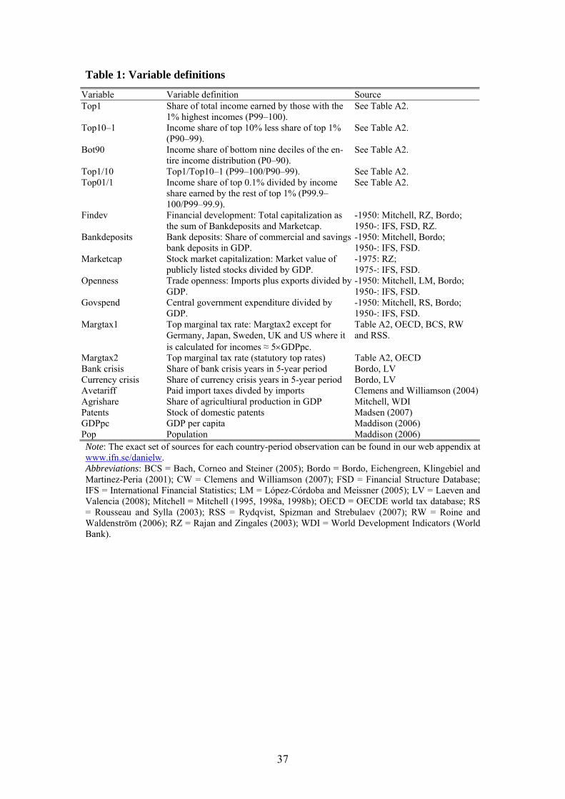
37

Table 1: Variable definitions

Variable Variable definition Source Top1 Share of total income earned by those with the

1% highest incomes (P99–100). See Table A2.

Top10–1 Income share of top 10% less share of top 1% (P90–99).

See Table A2.

Bot90 Income share of bottom nine deciles of the en-tire income distribution (P0–90).

See Table A2.

Top1/10 Top1/Top10–1 (P99–100/P90–99). See Table A2. Top01/1 Income share of top 0.1% divided by income

share earned by the rest of top 1% (P99.9–100/P99–99.9).

See Table A2.

Findev Financial development: Total capitalization as the sum of Bankdeposits and Marketcap.

-1950: Mitchell, RZ, Bordo; 1950-: IFS, FSD, RZ.

Bankdeposits Bank deposits: Share of commercial and savings bank deposits in GDP.

-1950: Mitchell, Bordo; 1950-: IFS, FSD.

Marketcap Stock market capitalization: Market value of publicly listed stocks divided by GDP.

-1975: RZ; 1975-: IFS, FSD.

Openness Trade openness: Imports plus exports divided by GDP.

-1950: Mitchell, LM, Bordo; 1950-: IFS, FSD.

Govspend Central government expenditure divided by GDP.

-1950: Mitchell, RS, Bordo; 1950-: IFS, FSD.

Margtax1 Top marginal tax rate: Margtax2 except for Germany, Japan, Sweden, UK and US where it is calculated for incomes ≈ 5×GDPpc.

Table A2, OECD, BCS, RW and RSS.

Margtax2 Top marginal tax rate (statutory top rates) Table A2, OECD Bank crisis Share of bank crisis years in 5-year period Bordo, LV Currency crisis Share of currency crisis years in 5-year period Bordo, LV Avetariff Paid import taxes divded by imports Clemens and Williamson (2004)Agrishare Share of agricultiural production in GDP Mitchell, WDI Patents Stock of domestic patents Madsen (2007) GDPpc GDP per capita Maddison (2006) Pop Population Maddison (2006) Note: The exact set of sources for each country-period observation can be found in our web appendix at www.ifn.se/danielw. Abbreviations: BCS = Bach, Corneo and Steiner (2005); Bordo = Bordo, Eichengreen, Klingebiel and Martinez-Peria (2001); CW = Clemens and Williamson (2007); FSD = Financial Structure Database; IFS = International Financial Statistics; LM = López-Córdoba and Meissner (2005); LV = Laeven and Valencia (2008); Mitchell = Mitchell (1995, 1998a, 1998b); OECD = OECDE world tax database; RS = Rousseau and Sylla (2003); RSS = Rydqvist, Spizman and Strebulaev (2007); RW = Roine and Waldenström (2006); RZ = Rajan and Zingales (2003); WDI = World Development Indicators (World Bank).

38

Table 2: Income inequality data No. 5-year periods

Country Source Full sample period Top1 Top10–1

Argentina Alvaredo (2009) 1932-1973a,1997-2004 9 0 Australia Atkinson and Leigh (2007) 1921-2002 17 13 Canada Saez and Veall (2007) 1920-2001 17 13 Finland Riiehlä et al. (2009) 1966-1985a,1990-2002 8 8 France Piketty (2007) 1915-1998 18 18 Germany Dell (2009) 1925-1938,1944-1998 13 13 India Banerjee and Piketty (2009) 1922-1999 16 0 Ireland Nolan (2009) 1938, 1943, 1965,1973-2000 8 8 Japan Moriguchi and Saez (2007) 1886-2002 21 17b Netherlands Atkinson and Salverda (2007) 1914-1999 17 17 New Zealand Atkinson and Leigh (2007) 1921-2002 17 17 Spain Alvaredo and Saez (2009) 1981-2002 5 5 Sweden Roine and Waldenström (2009) 1903-1935a,1941-2004 20 20 Switzerland Dell et al. (2007) 1933-1996 14 14 United Kingdom Atkinson and Salverda (2007) 1908-1999 14 14 United States Piketty and Saez (2007) 1913-2002 19 18

a There are years with missing values in this subperiod b The shares-within-shares data for Japan is based on the top five percent (P95–100).

Table 3: Summary statistcs for our main variables.

Variable Obs Mean Std. Dev. Min Max Top1 237 10.69 4.68 2.95 26.99 Top10–1 182 23.36 2.89 16.00 30.68 Bot90 182 66.76 5.99 49.86 81.05 Top1/10 199 0.45 0.24 0.18 1.63 Top01/1 236 0.46 0.17 0.17 0.93 GDPpc 508 7273 6070 513 28581 Pop 516 82073 181844 847 1287576 Govspend 475 0.14 0.06 0.01 0.49 Findev 280 0.94 0.54 0.06 3.61 Openness 446 0.40 0.36 0.02 3.66 Margtax1 131 0.53 0.13 0.22 0.86 Tariffs 411 0.10 0.08 0.01 0.48 Bankdeposits 461 0.44 0.26 0.00 1.56 Marketcap 283 0.48 0.43 0.00 2.32 Privatecredit 264 0.60 0.39 0.04 1.95 Bank crisis 357 0.05 0.15 0.00 1.00 Currency crisis 357 0.06 0.12 0.00 0.60 Agrishare 296 16.34 14.50 1.00 61.00 Patents 399 14122 40091 3 370677

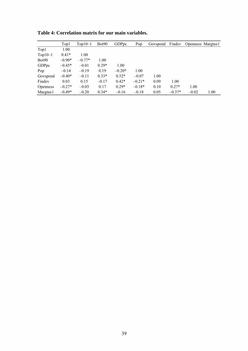
39

Table 4: Correlation matrix for our main variables.

Top1 Top10–1 Bot90 GDPpc Pop Govspend Findev Openness Margtax1Top1 1.00 Top10–1 0.41* 1.00 Bot90 –0.90* –0.77* 1.00 GDPpc –0.45* –0.01 0.29* 1.00 Pop –0.14 –0.19 0.19 –0.20* 1.00 Govspend –0.40* –0.11 0.33* 0.52* –0.07 1.00 Findev 0.03 0.15 –0.17 0.42* –0.21* 0.09 1.00 Openness –0.27* –0.03 0.17 0.29* –0.18* 0.10 0.27* 1.00 Margtax1 –0.49* –0.20 0.34* –0.16 –0.18 0.05 –0.37* –0.02 1.00

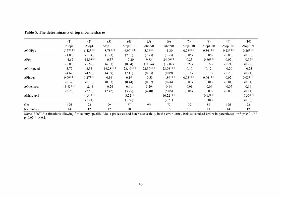
40

Table 5. The determinants of top income shares

(1) (2) (3) (4) (5) (6) (7) (8) (9) (10) Δtop1 Δtop1 Δtop10–1 Δtop10–1 Δbot90 Δbot90 Δtop1/10 Δtop1/10 Δtop01/1 Δtop01/1 ΔGDPpc 5.77*** 6.42*** –8.78*** –6.90*** 5.56** –1.30 0.28*** 0.36*** 0.23*** 0.26*** (1.03) (1.34) (1.73) (2.61) (2.73) (3.53) (0.05) (0.06) (0.05) (0.06) ΔPop –4.62 –12.98** –0.57 –12.20 9.83 24.09** –0.23 –0.66*** 0.02 –0.37* (5.03) (5.62) (6.31) (8.04) (11.54) (12.02) (0.22) (0.22) (0.21) (0.22) ΔGovspend 5.77 3.35 –16.28*** –23.40*** 22.39*** 23.96*** –0.10 0.12 –0.20 –0.25 (4.62) (4.66) (4.99) (7.11) (8.53) (8.89) (0.18) (0.19) (0.20) (0.21) ΔFindev 0.99*** 1.27*** 0.16 0.19 –0.53 –1.89*** 0.03*** 0.06*** 0.02 0.03*** (0.32) (0.30) (0.33) (0.44) (0.62) (0.66) (0.01) (0.01) (0.01) (0.01) ΔOpenness –8.83*** –2.46 –0.24 0.41 3.29 0.14 –0.01 –0.06 –0.07 0.14 (2.26) (2.55) (2.42) (3.75) (4.40) (5.05) (0.08) (0.09) (0.09) (0.11) ΔMargtax1 –4.34*** –3.22** 10.22*** –0.15*** –0.30*** (1.21) (1.56) (2.21) (0.04) (0.05) Obs 126 92 99 77 99 77 109 87 126 92 N countries 14 12 12 10 12 10 13 11 14 12 Notes: FDGLS estimations allowing for country specific AR(1) processes and heteroskedasticity in the error terms. Robust standard errors in parentheses. *** p<0.01, ** p<0.05, * p<0.1.

41

Table 6. The effects at different levels of economic development (1) (2) (3) (4) Δtop1 Δtop1 Δtop10–1 Δtop10–1 ΔGDPpc 5.39*** –8.52*** (1.06) (1.71) ΔPop –4.90 –5.86 –2.78 4.16 (5.03) (5.18) (6.64) (6.44) ΔGovspend 3.38 5.75 –17.79*** –18.87*** (4.72) (4.65) (5.39) (4.83) ΔFindev 1.05*** 0.20 (0.33) (0.33) ΔOpenness –9.15*** –8.49*** –0.34 –0.78 (2.26) (2.26) (2.45) (2.31) ΔGDPpc×Lowdev 5.04*** –9.02*** (1.13) (2.08) ΔGDPpc×Meddev 6.37*** –7.32*** (1.50) (2.40) ΔGDPpc×Highdev 2.45 –9.77*** (2.26) (2.69) ΔFindev×Lowdev 1.67* –3.27** (0.94) (1.37) ΔFindev×Meddev 0.88* 0.33 (0.52) (0.63) ΔFindev×Highdev 0.86* 0.38 (0.44) (0.37) F–test: Low=Meda 0.31 0.45 0.52 0.02 F–test: Low=Higha 0.25 0.42 0.80 0.01 F–test: Med=Higha 0.07 0.98 0.34 0.94 Obs 126 126 99 99 N countries 14 14 12 12 Notes: Interactions between low, medium and high GDP per capita and ΔGDPpc and ΔFindev. See also the notes of Table 5. a P–value of an F–test of equality of coefficients.

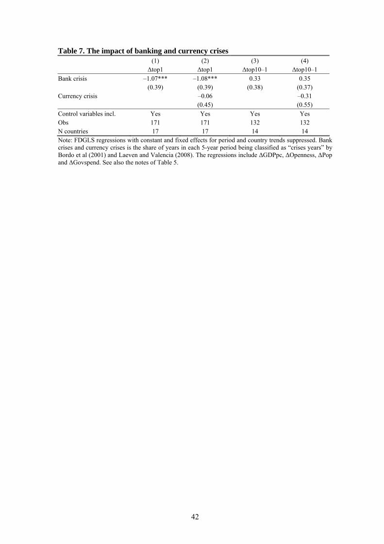
42

Table 7. The impact of banking and currency crises (1) (2) (3) (4) Δtop1 Δtop1 Δtop10–1 Δtop10–1 Bank crisis –1.07*** –1.08*** 0.33 0.35 (0.39) (0.39) (0.38) (0.37) Currency crisis –0.06 –0.31 (0.45) (0.55) Control variables incl. Yes Yes Yes Yes Obs 171 171 132 132 N countries 17 17 14 14 Note: FDGLS regressions with constant and fixed effects for period and country trends suppressed. Bank crises and currency crises is the share of years in each 5-year period being classified as “crises years” by Bordo et al (2001) and Laeven and Valencia (2008). The regressions include ΔGDPpc, ΔOpenness, ΔPop and ΔGovspend. See also the notes of Table 5.

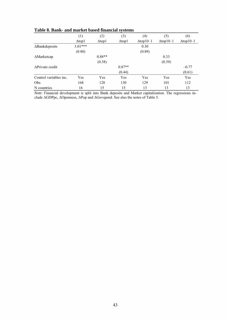
43

Table 8. Bank- and market based financial systems (1) (2) (3) (4) (5) (6) Δtop1 Δtop1 Δtop1 Δtop10–1 Δtop10–1 Δtop10–1 ΔBankdeposits 3.01*** 0.30 (0.80) (0.89) ΔMarketcap 0.88** 0.33 (0.38) (0.39) ΔPrivate credit 0.87** –0.77 (0.44) (0.61) Control variables inc. Yes Yes Yes Yes Yes Yes Obs 168 128 130 129 101 112 N countries 16 15 15 13 13 13 Note: Financial development is split into Bank deposits and Market capitalization. The regressions in-clude ΔGDPpc, ΔOpenness, ΔPop and ΔGovspend. See also the notes of Table 5.

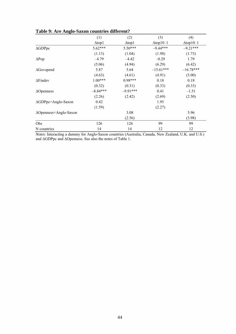
44

Table 9: Are Anglo-Saxon countries different? (1) (2) (3) (4) Δtop1 Δtop1 Δtop10–1 Δtop10–1 ΔGDPpc 5.62*** 5.50*** –9.44*** –9.21*** (1.13) (1.04) (1.98) (1.73) ΔPop –4.79 –4.42 –0.29 1.79 (5.06) (4.94) (6.29) (6.42) ΔGovspend 5.87 5.64 –15.61*** –16.78*** (4.63) (4.61) (4.91) (5.00) ΔFindev 1.00*** 0.98*** 0.18 0.18 (0.32) (0.31) (0.33) (0.33) ΔOpenness –8.84*** –9.91*** 0.41 –1.51 (2.26) (2.42) (2.69) (2.50) ΔGDPpc×Anglo-Saxon 0.42 1.95 (1.59) (2.27) ΔOpenness×Anglo-Saxon 3.08 5.96 (2.56) (3.98) Obs 126 126 99 99 N countries 14 14 12 12 Notes: Interacting a dummy for Anglo-Saxon countries (Australia, Canada, New Zealand, U.K. and U.S.) and ΔGDPpc and ΔOpenness. See also the notes of Table 1.

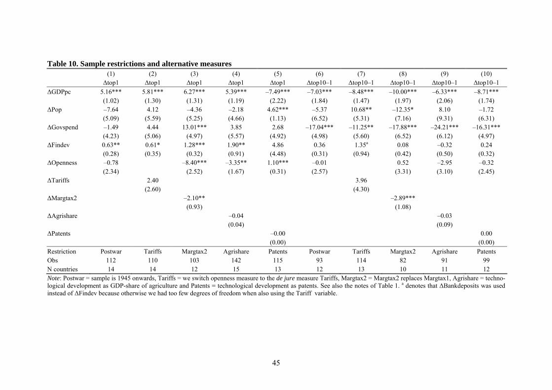
45

Table 10. Sample restrictions and alternative measures (1) (2) (3) (4) (5) (6) (7) (8) (9) (10) Δtop1 Δtop1 Δtop1 Δtop1 Δtop1 Δtop10–1 Δtop10–1 Δtop10–1 Δtop10–1 Δtop10–1 ΔGDPpc 5.16*** 5.81*** 6.27*** 5.39*** –7.49*** –7.03*** –8.48*** –10.00*** –6.33*** –8.71*** (1.02) (1.30) (1.31) (1.19) (2.22) (1.84) (1.47) (1.97) (2.06) (1.74) ΔPop –7.64 4.12 –4.36 –2.18 4.62*** –5.37 10.68** –12.35* 8.10 –1.72 (5.09) (5.59) (5.25) (4.66) (1.13) (6.52) (5.31) (7.16) (9.31) (6.31) ΔGovspend –1.49 4.44 13.01*** 3.85 2.68 –17.04*** –11.25** –17.88*** –24.21*** –16.31*** (4.23) (5.06) (4.97) (5.57) (4.92) (4.98) (5.60) (6.52) (6.12) (4.97) ΔFindev 0.63** 0.61* 1.28*** 1.90** 4.86 0.36 1.35a 0.08 –0.32 0.24 (0.28) (0.35) (0.32) (0.91) (4.48) (0.31) (0.94) (0.42) (0.50) (0.32) ΔOpenness –0.78 –8.40*** –3.35** 1.10*** –0.01 0.52 –2.95 –0.32 (2.34) (2.52) (1.67) (0.31) (2.57) (3.31) (3.10) (2.45) ΔTariffs 2.40 3.96 (2.60) (4.30) ΔMargtax2 –2.10** –2.89*** (0.93) (1.08) ΔAgrishare –0.04 –0.03 (0.04) (0.09) ΔPatents –0.00 0.00 (0.00) (0.00) Restriction Postwar Tariffs Margtax2 Agrishare Patents Postwar Tariffs Margtax2 Agrishare Patents Obs 112 110 103 142 115 93 114 82 91 99 N countries 14 14 12 15 13 12 13 10 11 12 Note: Postwar = sample is 1945 onwards, Tariffs = we switch openness measure to the de jure measure Tariffs, Margtax2 = Margtax2 replaces Margtax1, Agrishare = techno-logical development as GDP-share of agriculture and Patents = technological development as patents. See also the notes of Table 1. a denotes that ΔBankdeposits was used instead of ΔFindev because otherwise we had too few degrees of freedom when also using the Tariff variable.

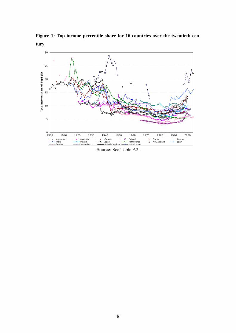
46

Figure 1: Top income percentile share for 16 countries over the twentieth cen-

tury.

0

5

10

15

20

25

30

1900 1910 1920 1930 1940 1950 1960 1970 1980 1990 2000

Tota

l in

com

e s

hare

of

Top

1 (

%)

Argentina Australia Canada Finland France GermanyIndia Ireland Japan Netherlands New Zealand SpainSweden Switzerland United Kingdom United States

Source: See Table A2.

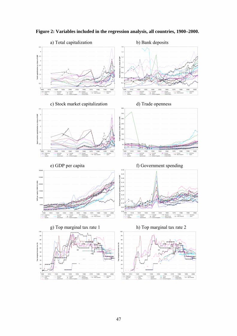
47

Figure 2: Variables included in the regression analysis, all countries, 1900–2000.

a) Total capitalization b) Bank deposits

0

0.5

1

1.5

2

2.5

3

3.5

4

4.5

1900 1910 1920 1930 1940 1950 1960 1970 1980 1990 2000

To

tal

cap

itali

zati

on

as s

hare

of

GD

P

Argentina Australia Canada Finland France GermanyIndia Ireland Japan Netherlands New Zealand SpainSweden Switzerland United Kingdom United States

0

0.2

0.4

0.6

0.8

1

1.2

1.4

1.6

1900 1910 1920 1930 1940 1950 1960 1970 1980 1990 2000

Ban

k d

ep

osit

s a

s s

hare

of

GD

P

Argentina Australia Canada Finland France GermanyIndia Ireland Japan Netherlands New Zealand SpainSweden Switzerland United Kingdom United States

c) Stock market capitalization d) Trade openness

0

0.5

1

1.5

2

2.5

3

3.5

1900 1910 1920 1930 1940 1950 1960 1970 1980 1990 2000

Sto

ck m

ark

et

cap

itali

zati

on

as

sh

are

of

GD

P

Argentina Australia Canada Finland France GermanyIndia Ireland Japan Netherlands New Zealand SpainSweden Switzerland United Kingdom United States

0

50

100

150

200

250

300

350

400

1900 1910 1920 1930 1940 1950 1960 1970 1980 1990 2000

Tra

de o

pen

ness

(tra

de s

hare

in

GD

P)

Argentina Australia Canada Finland France GermanyIndia Ireland Japan Netherlands New Zealand SpainSweden Switzerland United Kingdom United States

e) GDP per capita f) Government spending

0

5000

10000

15000

20000

25000

30000

1900 1910 1920 1930 1940 1950 1960 1970 1980 1990 2000

GD

P p

er

cap

ita (

1990 G

-K U

SD)

Argentina Australia Canada Finland France GermanyIndia Ireland Japan Netherlands New Zealand SpainSweden Switzerland United Kingdom United States

0.00

0.05

0.10

0.15

0.20

0.25

0.30

0.35

0.40

0.45

0.50

1900 1910 1920 1930 1940 1950 1960 1970 1980 1990 2000

Cen

tral

govern

men

t sp

en

din

g a

s sh

are

of

GD

P

Argentina Australia Canada Finland France GermanyIndia Ireland Japan Netherlands New Zealand SpainSweden Switzerland United Kingdom United States

g) Top marginal tax rate 1 h) Top marginal tax rate 2

0

10

20

30

40

50

60

70

80

90

100

1900 1910 1920 1930 1940 1950 1960 1970 1980 1990 2000

Top

marg

inal in

com

e t

ax (

%)

Argentina Australia Canada Finland France GermanyIndia Ireland Japan Netherlands New Zealand SpainSweden Switzerland United Kingdom United States

0

10

20

30

40

50

60

70

80

90

100

1900 1910 1920 1930 1940 1950 1960 1970 1980 1990 2000

Top

marg

inal in

com

e t

ax (

%)

Argentina Australia Canada China Finland FranceGermany India Ireland Japan Netherlands New ZealandSpain Sweden Switzerland United Kingdom United States

48

Figure 3. Anglo-Saxon deviations from common time trend

-3

-2

-1

0

1

2

3

4

5

1955 1960 1965 1970 1975 1980 1985 1990 1995 2000

Co

eff

icie

nt

est

imate

s an

d s

tan

dard

err

ors

Anglo-saxon period effects without controls Anglo-saxon period effects with controls Note: The graph displays the interaction terms between time fixed effects and an Anglo-Saxon dummy, with and without our base set of control variables. 95 percent confidence intervals indicated.

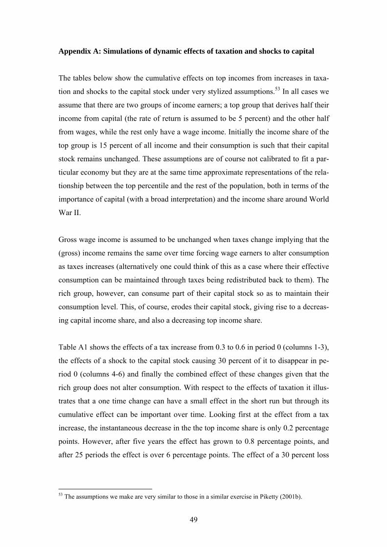
49

Appendix A: Simulations of dynamic effects of taxation and shocks to capital

The tables below show the cumulative effects on top incomes from increases in taxa-

tion and shocks to the capital stock under very stylized assumptions.53 In all cases we

assume that there are two groups of income earners; a top group that derives half their

income from capital (the rate of return is assumed to be 5 percent) and the other half

from wages, while the rest only have a wage income. Initially the income share of the

top group is 15 percent of all income and their consumption is such that their capital

stock remains unchanged. These assumptions are of course not calibrated to fit a par-

ticular economy but they are at the same time approximate representations of the rela-

tionship between the top percentile and the rest of the population, both in terms of the

importance of capital (with a broad interpretation) and the income share around World

War II.

Gross wage income is assumed to be unchanged when taxes change implying that the

(gross) income remains the same over time forcing wage earners to alter consumption

as taxes increases (alternatively one could think of this as a case where their effective

consumption can be maintained through taxes being redistributed back to them). The

rich group, however, can consume part of their capital stock so as to maintain their

consumption level. This, of course, erodes their capital stock, giving rise to a decreas-

ing capital income share, and also a decreasing top income share.

Table A1 shows the effects of a tax increase from 0.3 to 0.6 in period 0 (columns 1-3),

the effects of a shock to the capital stock causing 30 percent of it to disappear in pe-

riod 0 (columns 4-6) and finally the combined effect of these changes given that the

rich group does not alter consumption. With respect to the effects of taxation it illus-

trates that a one time change can have a small effect in the short run but through its

cumulative effect can be important over time. Looking first at the effect from a tax

increase, the instantaneous decrease in the the top income share is only 0.2 percentage

points. However, after five years the effect has grown to 0.8 percentage points, and

after 25 periods the effect is over 6 percentage points. The effect of a 30 percent loss

53 The assumptions we make are very similar to those in a similar exercise in Piketty (2001b).

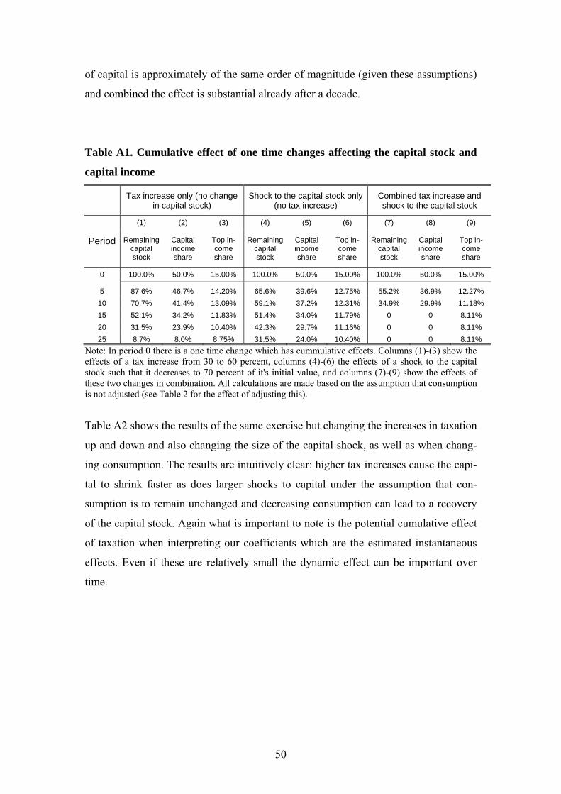
50

of capital is approximately of the same order of magnitude (given these assumptions)

and combined the effect is substantial already after a decade.

Table A1. Cumulative effect of one time changes affecting the capital stock and

capital income

Tax increase only (no change in capital stock)

Shock to the capital stock only (no tax increase)

Combined tax increase and shock to the capital stock

(1) (2) (3) (4) (5) (6) (7) (8) (9)

Period Remaining capital stock

Capital income share

Top in-come share

Remaining capital stock

Capital income share

Top in-come share

Remaining capital stock

Capital income share

Top in-come share

0 100.0% 50.0% 15.00% 100.0% 50.0% 15.00% 100.0% 50.0% 15.00%

5 87.6% 46.7% 14.20% 65.6% 39.6% 12.75% 55.2% 36.9% 12.27% 10 70.7% 41.4% 13.09% 59.1% 37.2% 12.31% 34.9% 29.9% 11.18% 15 52.1% 34.2% 11.83% 51.4% 34.0% 11.79% 0 0 8.11% 20 31.5% 23.9% 10.40% 42.3% 29.7% 11.16% 0 0 8.11% 25 8.7% 8.0% 8.75% 31.5% 24.0% 10.40% 0 0 8.11%

Note: In period 0 there is a one time change which has cummulative effects. Columns (1)-(3) show the effects of a tax increase from 30 to 60 percent, columns (4)-(6) the effects of a shock to the capital stock such that it decreases to 70 percent of it's initial value, and columns (7)-(9) show the effects of these two changes in combination. All calculations are made based on the assumption that consumption is not adjusted (see Table 2 for the effect of adjusting this).

Table A2 shows the results of the same exercise but changing the increases in taxation

up and down and also changing the size of the capital shock, as well as when chang-

ing consumption. The results are intuitively clear: higher tax increases cause the capi-

tal to shrink faster as does larger shocks to capital under the assumption that con-

sumption is to remain unchanged and decreasing consumption can lead to a recovery

of the capital stock. Again what is important to note is the potential cumulative effect

of taxation when interpreting our coefficients which are the estimated instantaneous

effects. Even if these are relatively small the dynamic effect can be important over

time.

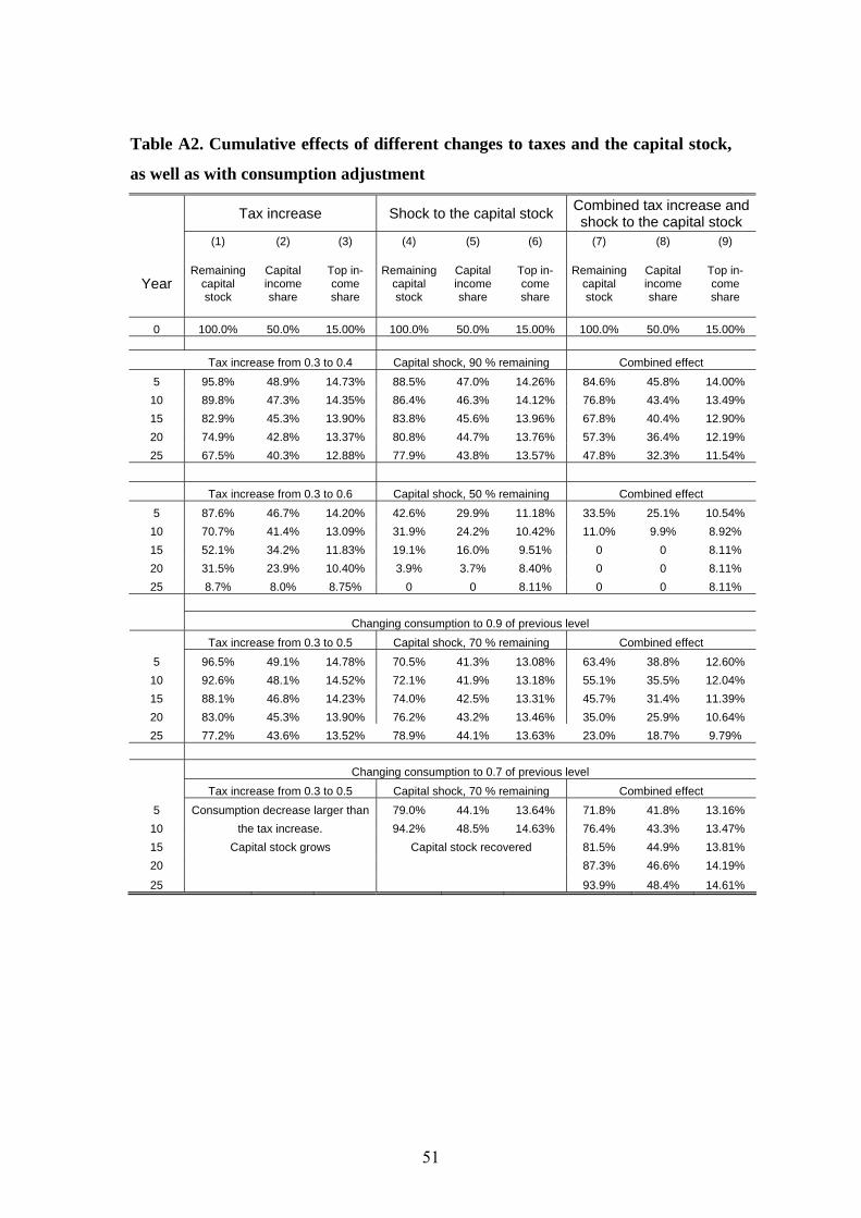
51

Table A2. Cumulative effects of different changes to taxes and the capital stock,

as well as with consumption adjustment

Tax increase Shock to the capital stock Combined tax increase and shock to the capital stock

(1) (2) (3) (4) (5) (6) (7) (8) (9)

Year Remaining

capital stock

Capital income share

Top in-come share

Remaining capital stock

Capital income share

Top in-come share

Remaining capital stock

Capital income share

Top in-come share

0 100.0% 50.0% 15.00% 100.0% 50.0% 15.00% 100.0% 50.0% 15.00% Tax increase from 0.3 to 0.4 Capital shock, 90 % remaining Combined effect 5 95.8% 48.9% 14.73% 88.5% 47.0% 14.26% 84.6% 45.8% 14.00%

10 89.8% 47.3% 14.35% 86.4% 46.3% 14.12% 76.8% 43.4% 13.49% 15 82.9% 45.3% 13.90% 83.8% 45.6% 13.96% 67.8% 40.4% 12.90% 20 74.9% 42.8% 13.37% 80.8% 44.7% 13.76% 57.3% 36.4% 12.19% 25 67.5% 40.3% 12.88% 77.9% 43.8% 13.57% 47.8% 32.3% 11.54%

Tax increase from 0.3 to 0.6 Capital shock, 50 % remaining Combined effect 5 87.6% 46.7% 14.20% 42.6% 29.9% 11.18% 33.5% 25.1% 10.54%

10 70.7% 41.4% 13.09% 31.9% 24.2% 10.42% 11.0% 9.9% 8.92% 15 52.1% 34.2% 11.83% 19.1% 16.0% 9.51% 0 0 8.11% 20 31.5% 23.9% 10.40% 3.9% 3.7% 8.40% 0 0 8.11% 25 8.7% 8.0% 8.75% 0 0 8.11% 0 0 8.11%

Changing consumption to 0.9 of previous level

Tax increase from 0.3 to 0.5 Capital shock, 70 % remaining Combined effect 5 96.5% 49.1% 14.78% 70.5% 41.3% 13.08% 63.4% 38.8% 12.60%

10 92.6% 48.1% 14.52% 72.1% 41.9% 13.18% 55.1% 35.5% 12.04% 15 88.1% 46.8% 14.23% 74.0% 42.5% 13.31% 45.7% 31.4% 11.39% 20 83.0% 45.3% 13.90% 76.2% 43.2% 13.46% 35.0% 25.9% 10.64% 25 77.2% 43.6% 13.52% 78.9% 44.1% 13.63% 23.0% 18.7% 9.79%

Changing consumption to 0.7 of previous level Tax increase from 0.3 to 0.5 Capital shock, 70 % remaining Combined effect 5 Consumption decrease larger than 79.0% 44.1% 13.64% 71.8% 41.8% 13.16%

10 the tax increase. 94.2% 48.5% 14.63% 76.4% 43.3% 13.47% 15 Capital stock grows Capital stock recovered 81.5% 44.9% 13.81% 20 87.3% 46.6% 14.19%

25 93.9% 48.4% 14.61%

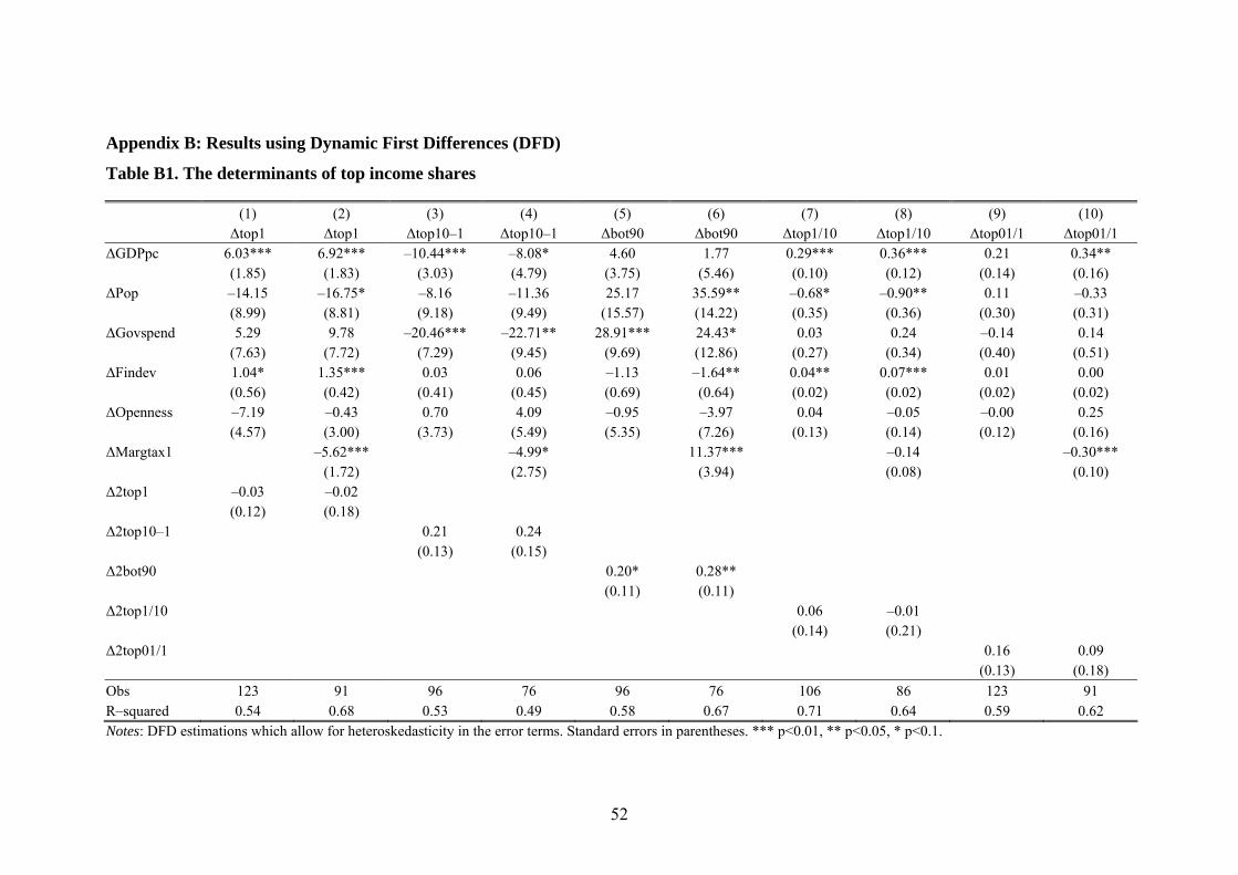
52

Appendix B: Results using Dynamic First Differences (DFD)

Table B1. The determinants of top income shares

(1) (2) (3) (4) (5) (6) (7) (8) (9) (10) Δtop1 Δtop1 Δtop10–1 Δtop10–1 Δbot90 Δbot90 Δtop1/10 Δtop1/10 Δtop01/1 Δtop01/1 ΔGDPpc 6.03*** 6.92*** –10.44*** –8.08* 4.60 1.77 0.29*** 0.36*** 0.21 0.34** (1.85) (1.83) (3.03) (4.79) (3.75) (5.46) (0.10) (0.12) (0.14) (0.16) ΔPop –14.15 –16.75* –8.16 –11.36 25.17 35.59** –0.68* –0.90** 0.11 –0.33 (8.99) (8.81) (9.18) (9.49) (15.57) (14.22) (0.35) (0.36) (0.30) (0.31) ΔGovspend 5.29 9.78 –20.46*** –22.71** 28.91*** 24.43* 0.03 0.24 –0.14 0.14 (7.63) (7.72) (7.29) (9.45) (9.69) (12.86) (0.27) (0.34) (0.40) (0.51) ΔFindev 1.04* 1.35*** 0.03 0.06 –1.13 –1.64** 0.04** 0.07*** 0.01 0.00 (0.56) (0.42) (0.41) (0.45) (0.69) (0.64) (0.02) (0.02) (0.02) (0.02) ΔOpenness –7.19 –0.43 0.70 4.09 –0.95 –3.97 0.04 –0.05 –0.00 0.25 (4.57) (3.00) (3.73) (5.49) (5.35) (7.26) (0.13) (0.14) (0.12) (0.16) ΔMargtax1 –5.62*** –4.99* 11.37*** –0.14 –0.30*** (1.72) (2.75) (3.94) (0.08) (0.10) Δ2top1 –0.03 –0.02 (0.12) (0.18) Δ2top10–1 0.21 0.24 (0.13) (0.15) Δ2bot90 0.20* 0.28** (0.11) (0.11) Δ2top1/10 0.06 –0.01 (0.14) (0.21) Δ2top01/1 0.16 0.09 (0.13) (0.18) Obs 123 91 96 76 96 76 106 86 123 91 R–squared 0.54 0.68 0.53 0.49 0.58 0.67 0.71 0.64 0.59 0.62 Notes: DFD estimations which allow for heteroskedasticity in the error terms. Standard errors in parentheses. *** p<0.01, ** p<0.05, * p<0.1.

53

Table B2. The effects at different levels of economic development (1) (2) (3) (4) Δtop1 Δtop1 Δtop10–1 Δtop10–1 ΔGDPpc 5.97*** –10.83*** (1.92) (3.01) ΔPop –14.82 –15.78* –7.89 –3.04 (9.08) (8.89) (9.20) (11.36) ΔGovspend 3.17 5.60 –21.10*** –21.95*** (7.85) (7.76) (7.77) (7.51) ΔFindev 1.09* 0.05 (0.59) (0.42) ΔOpenness –7.63 –7.26 0.83 0.44 (4.61) (4.66) (3.89) (3.77) ΔGDPpc×Lowdev 5.84*** –9.63** (1.86) (3.71) ΔGDPpc×Meddev 6.89*** –10.72*** (2.30) (3.43) ΔGDPpc×Highdev 4.09 –11.93*** (3.52) (4.05) ΔFindev×Lowdev 1.75 –1.97 (1.39) (2.13) ΔFindev×Meddev 1.29** –0.22 (0.54) (0.59) ΔFindev×Highdev 0.74 0.71 (0.75) (0.51) Δ2top1 –0.02 –0.02 (0.12) (0.12) Δ2top10–1 0.22 0.21 (0.15) (0.13) F–test: Low=Meda 0.56 0.74 0.73 0.45 F–test: Low=Higha 0.64 0.48 0.60 0.23 F–test: Med=Higha 0.40 0.49 0.70 0.21 Obs 123 123 96 96 R–squared 0.55 0.55 0.53 0.55 Notes: Interactions between low, medium and high GDP per capita and ΔGDPpc and ΔFindev. See also the notes of Table 1. a P–value from an F–test of equality of coefficients.

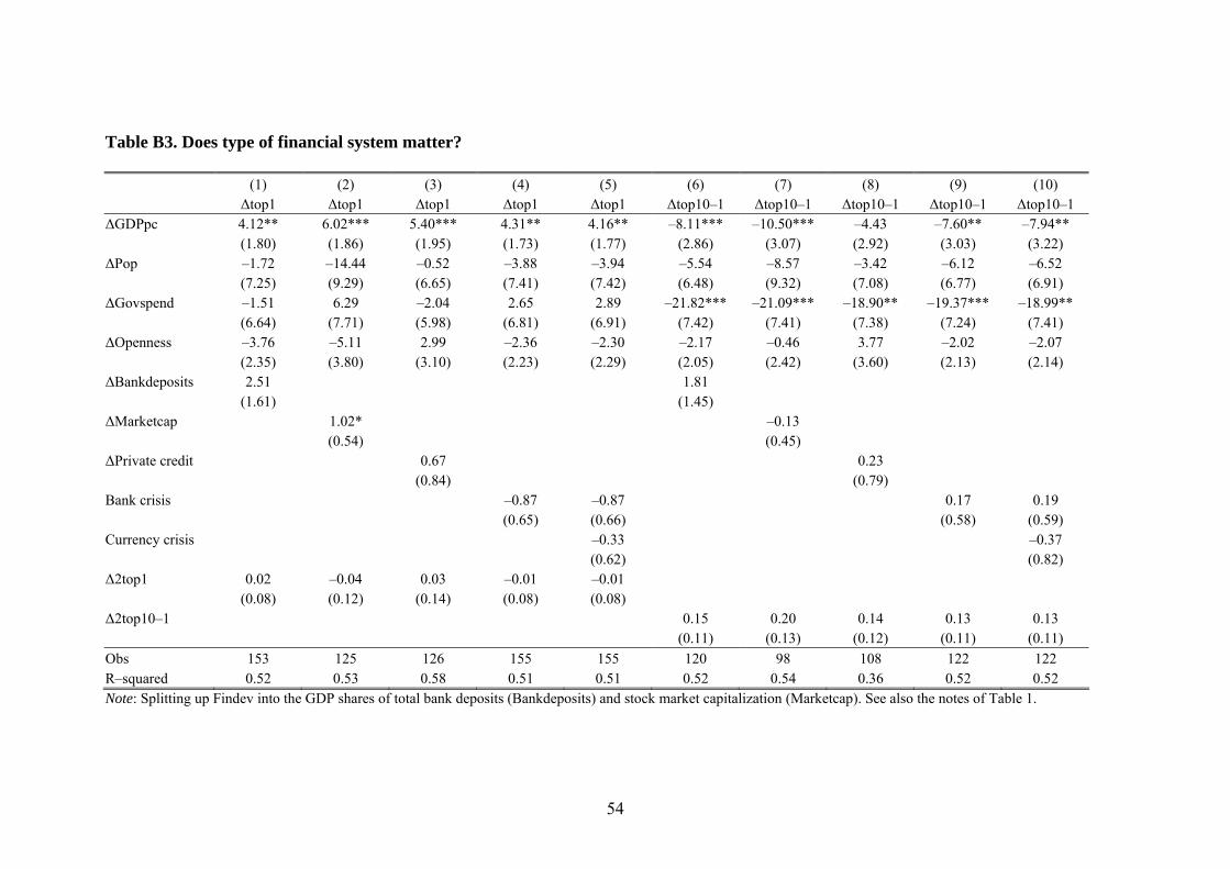
54

Table B3. Does type of financial system matter? (1) (2) (3) (4) (5) (6) (7) (8) (9) (10) Δtop1 Δtop1 Δtop1 Δtop1 Δtop1 Δtop10–1 Δtop10–1 Δtop10–1 Δtop10–1 Δtop10–1 ΔGDPpc 4.12** 6.02*** 5.40*** 4.31** 4.16** –8.11*** –10.50*** –4.43 –7.60** –7.94** (1.80) (1.86) (1.95) (1.73) (1.77) (2.86) (3.07) (2.92) (3.03) (3.22) ΔPop –1.72 –14.44 –0.52 –3.88 –3.94 –5.54 –8.57 –3.42 –6.12 –6.52 (7.25) (9.29) (6.65) (7.41) (7.42) (6.48) (9.32) (7.08) (6.77) (6.91) ΔGovspend –1.51 6.29 –2.04 2.65 2.89 –21.82*** –21.09*** –18.90** –19.37*** –18.99** (6.64) (7.71) (5.98) (6.81) (6.91) (7.42) (7.41) (7.38) (7.24) (7.41) ΔOpenness –3.76 –5.11 2.99 –2.36 –2.30 –2.17 –0.46 3.77 –2.02 –2.07 (2.35) (3.80) (3.10) (2.23) (2.29) (2.05) (2.42) (3.60) (2.13) (2.14) ΔBankdeposits 2.51 1.81 (1.61) (1.45) ΔMarketcap 1.02* –0.13 (0.54) (0.45) ΔPrivate credit 0.67 0.23 (0.84) (0.79) Bank crisis –0.87 –0.87 0.17 0.19 (0.65) (0.66) (0.58) (0.59) Currency crisis –0.33 –0.37 (0.62) (0.82) Δ2top1 0.02 –0.04 0.03 –0.01 –0.01 (0.08) (0.12) (0.14) (0.08) (0.08) Δ2top10–1 0.15 0.20 0.14 0.13 0.13 (0.11) (0.13) (0.12) (0.11) (0.11) Obs 153 125 126 155 155 120 98 108 122 122 R–squared 0.52 0.53 0.58 0.51 0.51 0.52 0.54 0.36 0.52 0.52 Note: Splitting up Findev into the GDP shares of total bank deposits (Bankdeposits) and stock market capitalization (Marketcap). See also the notes of Table 1.

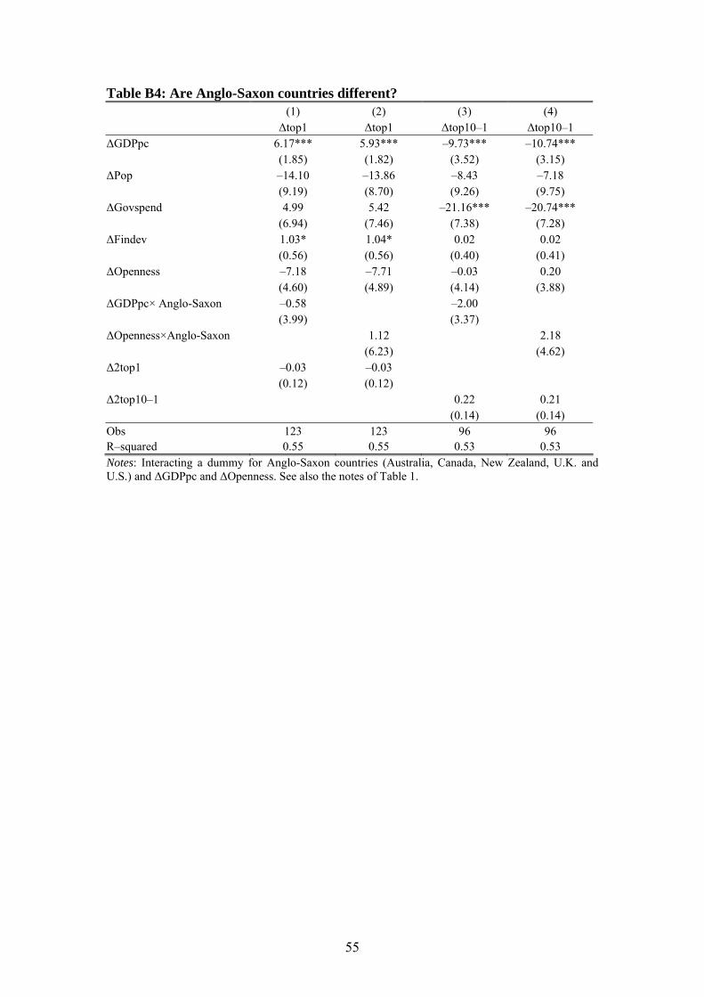
55

Table B4: Are Anglo-Saxon countries different? (1) (2) (3) (4) Δtop1 Δtop1 Δtop10–1 Δtop10–1 ΔGDPpc 6.17*** 5.93*** –9.73*** –10.74*** (1.85) (1.82) (3.52) (3.15) ΔPop –14.10 –13.86 –8.43 –7.18 (9.19) (8.70) (9.26) (9.75) ΔGovspend 4.99 5.42 –21.16*** –20.74*** (6.94) (7.46) (7.38) (7.28) ΔFindev 1.03* 1.04* 0.02 0.02 (0.56) (0.56) (0.40) (0.41) ΔOpenness –7.18 –7.71 –0.03 0.20 (4.60) (4.89) (4.14) (3.88) ΔGDPpc× Anglo-Saxon –0.58 –2.00 (3.99) (3.37) ΔOpenness×Anglo-Saxon 1.12 2.18 (6.23) (4.62) Δ2top1 –0.03 –0.03 (0.12) (0.12) Δ2top10–1 0.22 0.21 (0.14) (0.14) Obs 123 123 96 96 R–squared 0.55 0.55 0.53 0.53 Notes: Interacting a dummy for Anglo-Saxon countries (Australia, Canada, New Zealand, U.K. and U.S.) and ΔGDPpc and ΔOpenness. See also the notes of Table 1.

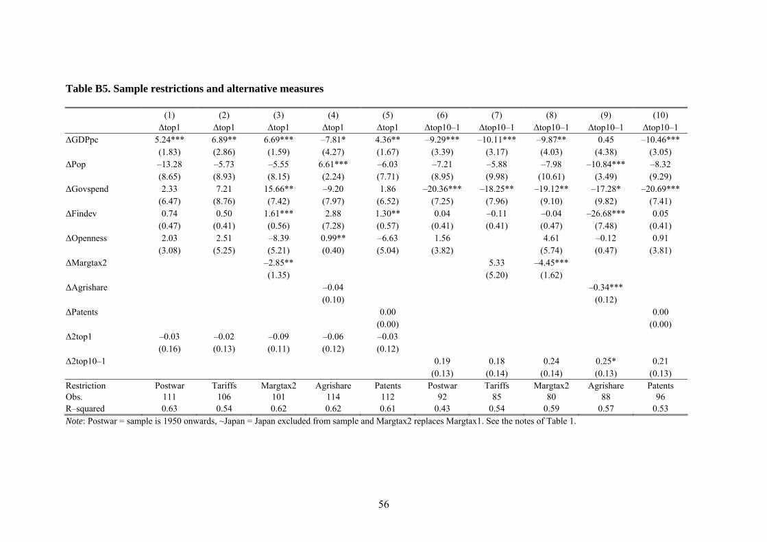
56

Table B5. Sample restrictions and alternative measures (1) (2) (3) (4) (5) (6) (7) (8) (9) (10) Δtop1 Δtop1 Δtop1 Δtop1 Δtop1 Δtop10–1 Δtop10–1 Δtop10–1 Δtop10–1 Δtop10–1 ΔGDPpc 5.24*** 6.89** 6.69*** –7.81* 4.36** –9.29*** –10.11*** –9.87** 0.45 –10.46*** (1.83) (2.86) (1.59) (4.27) (1.67) (3.39) (3.17) (4.03) (4.38) (3.05) ΔPop –13.28 –5.73 –5.55 6.61*** –6.03 –7.21 –5.88 –7.98 –10.84*** –8.32 (8.65) (8.93) (8.15) (2.24) (7.71) (8.95) (9.98) (10.61) (3.49) (9.29) ΔGovspend 2.33 7.21 15.66** –9.20 1.86 –20.36*** –18.25** –19.12** –17.28* –20.69*** (6.47) (8.76) (7.42) (7.97) (6.52) (7.25) (7.96) (9.10) (9.82) (7.41) ΔFindev 0.74 0.50 1.61*** 2.88 1.30** 0.04 –0.11 –0.04 –26.68*** 0.05 (0.47) (0.41) (0.56) (7.28) (0.57) (0.41) (0.41) (0.47) (7.48) (0.41) ΔOpenness 2.03 2.51 –8.39 0.99** –6.63 1.56 4.61 –0.12 0.91 (3.08) (5.25) (5.21) (0.40) (5.04) (3.82) (5.74) (0.47) (3.81) ΔMargtax2 –2.85** 5.33 –4.45*** (1.35) (5.20) (1.62) ΔAgrishare –0.04 –0.34*** (0.10) (0.12) ΔPatents 0.00 0.00 (0.00) (0.00) Δ2top1 –0.03 –0.02 –0.09 –0.06 –0.03 (0.16) (0.13) (0.11) (0.12) (0.12) Δ2top10–1 0.19 0.18 0.24 0.25* 0.21 (0.13) (0.14) (0.14) (0.13) (0.13) Restriction Postwar Tariffs Margtax2 Agrishare Patents Postwar Tariffs Margtax2 Agrishare Patents Obs. 111 106 101 114 112 92 85 80 88 96 R–squared 0.63 0.54 0.62 0.62 0.61 0.43 0.54 0.59 0.57 0.53 Note: Postwar = sample is 1950 onwards, ~Japan = Japan excluded from sample and Margtax2 replaces Margtax1. See the notes of Table 1.