risk-taking, inequality and output in the long-run · risk-taking, inequality and output in the...
TRANSCRIPT
Risk-Taking, Inequality and Output in
the Long-Run
Shuhei Aoki*
Makoto Nirei** [email protected]
Kazufumi Yamana***
No.18-E-4 March 2018
Bank of Japan 2-1-1 Nihonbashi-Hongokucho, Chuo-ku, Tokyo 103-0021, Japan
* Shinshu University
*** University of Tokyo
*** Kanagawa University
Papers in the Bank of Japan Working Paper Series are circulated in order to stimulate discussion
and comments. Views expressed are those of authors and do not necessarily reflect those of
the Bank.
If you have any comment or question on the working paper series, please contact each author.
When making a copy or reproduction of the content for commercial purposes, please contact the
Public Relations Department ([email protected]) at the Bank in advance to request
permission. When making a copy or reproduction, the source, Bank of Japan Working Paper
Series, should explicitly be credited.
Bank of Japan Working Paper Series

Risk-Taking, Inequality and Output in the Long-Run
Shuhei Aoki
Shinshu University
Makoto Nirei∗
University of Tokyo
Kazufumi Yamana
Kanagawa University
February 27, 2018
Abstract
We develop a tractable dynamic general equilibrium model with incomplete markets
for business risk sharing, which allows for analytical characterization under Epstein-Zin
preference with unitary elasticity of intertemporal substitution and Cobb-Douglas tech-
nology. Household stationary wealth dispersion is shown to follow a Pareto distribution.
In this environment, we conduct comparative statics of stationary output and house-
hold inequality when the cost of business risk sharing is reduced. Enhanced risk-taking
results in greater long-run outputs and real wage and a lower risk-free interest rate,
while its impact on inequality is ambiguous. A quantitative analysis under the parame-
ter values calibrated to Japanese economy shows that elimination of purchase costs for
mutual funds leads to an increase in output by 1.3 percent, a decrease in risk-free rate
by 15 basis points, and an increase in Gini coefficient of wealth in 2 percentage points.
Keywords: Financial development, risk-free rate, safe asset, Pareto distribution, depos-
itory institutions, mutual funds
JEL classification code: E2, G2
∗Address: 7-3-1 Hongo, Bunkyo-ku, Tokyo 113-0033, Japan. Email: [email protected]. This paper
was presented at the Seventh Joint Conference organized by the University of Tokyo Center for Advanced
Research in Finance and the Bank of Japan Research and Statistics Department in November 2017. We are
grateful to Shuhei Takahashi and conference participants for useful comments.
1
1 Introduction
The Japanese government has promoted a policy agenda of “from savings to asset building”
(and its predecessor, “from savings to investment”) policy. In an effort to promote economic
growth in a rapidly aging society, the main purposes of this agenda are to motivate Japanese
households, who have historically held most of their assets in savings deposits, to move into
long-term investment in risky equities, as well as to lighten the burden on the public pension
system (Financial Services Agency, 2016). The policy efforts include the introduction of
defined contribution individual pension plans (DC) and tax incentives for risky portfolios
(NISA). These policies are expected to decrease the cost of investment in risky equities and
thus induce households to shoulder a larger share of business risk.
In this paper, we investigate the macroeconomic consequences of these policies. We are
especially concerned with the quantitative effects of these policies on long-run output and
household inequality. By encouraging households to embrace a portfolio which takes on more
risk, the policy allows businesses to enjoy easier access to risky funds. The risks borne by
households also result in the dispersion of ex-post wealth among ex-ante identical households.
The policy also affects financial intermediaries, such as banks, which transform risky assets
into risk-less deposits that meet the demand from households for safe assets. Hence, the
policy also creates side-effects resulting from a risk-free rate. A general equilibrium model is
necessary to evaluate the overall effects of this policy.
To facilitate the analysis, we develop a tractable Bewley-type heterogenous-agent dy-
namic general equilibrium model which incorporates incomplete markets for risk-sharing.
In the model, households can hold three kinds of assets: (i) individual stock, that is, the
shares of a firm, (ii) a mutual fund composed of a finite number of individual stocks, and
(iii) risk-free asset. The risk-free asset is provided by financial intermediaries which pool a
continuum of individual stocks, as well as by the government who issues bonds. The indi-
vidual stocks conceptually capture individual stock as well as entrepreneurial investment in
self-employment. The individual stock is a high-risk, high-return asset, while the mutual
fund is a middle risk, middle-return asset and the risk-free asset is a zero-risk, low-return
2
asset. In the model, the returns are different because transaction costs are incurred when
households buy the mutual fund or risk-free asset.
Using the model, we analyze the effect of a policy change in which the transaction cost
of the mutual fund is decreased. There are two main channels influencing the inequality
of households. The first is a portfolio shift from the individual stock to the mutual fund.
By decreasing the volatility of household wealth, this channel contributes to the decrease in
inequality. The second main channel is a portfolio shift from the risk-free asset to the mutual
fund. This channel contributes to the increase in inequality. We conduct quantitative analysis
to clarify which channel has a stronger effect and whether inequality widens or shrinks as a
result of the policy change. Moreover, we analyze whether the reduction in the transaction
cost of the mutual fund promotes physical investment and increases output.
This paper’s contribution to existing literature is three-fold. First, we provide a formal
general equilibrium analysis of the limited participation in stock markets of Japanese house-
holds and the policy agenda which favors household risk-taking. While much has been dis-
cussed on this policy issue, no study has employed a dynamic general equilibrium framework
to our knowledge. Rather than modeling the limited participation per se as in Attanasio and
Paiella (2011) who focused on reconciling consumer theory and asset pricing, we introduce
a rate-of-return cost to account for the average risk-taking bahevior in a tractable Bewley
model such as in Angeletos and Calvet (2006), and explore general equilibrium implications
of the financial costs.
Second, this paper explores to what extent financial developments affect the income and
wealth inequality in a Bewley economy. On one hand, studies such as Nirei and Souma
(2007), Benhabib et al. (2011), and Jones (2015) have highlighted the importance of rate-
of-return risks in accounting for the right tail of income and wealth distributions. On the
other hand, authors such as Acemoglu et al. (2006) and Aoki et al. (2017) note that as an
economy approaches the world technology frontier, growth requires risky innovation activities.
Such an argument lies in the background of the risk-taking policy agenda in the context of
Japanese economy. This paper quantitatively assesses the policy’s impact on inequality
among households.
3
The third point touches on the broader discussion of how financial developments have
affected a risk-free rate. In our paper, we keep banks’ intermediary technology unchanged,
and ask what happens when the transaction costs of direct risk-taking by households are
reduced. The output is increased, in accordance with Obstfeld (1994) who argued that world
financial developments enhanced risk-taking through diversification of rate-of-return risks
and spurred growth. As a side-effect, we find that the risk-free rate is lowered. This suggests
a mechanism in which world financial developments contribute to lowering the risk-free rate,
if the banking technology remains unchanged. Moreover, the same mechanism suggests that
an economy with lower costs on direct risk-taking exhibits lower demand for risk-free assets.
Our analysis quantifies these effects of financial transaction costs on the risk-free rate and
safe-asset demand.
The rest of the paper is organized as follows. Section 2 presents the dynamic general
equilibrium model. Section 3 characterizes a stationary equilibrium analytically. Section
4 investigates one of the impacts of reduced costs for risk sharing quantitatively. Finally,
Section 5 concludes.
2 Model
2.1 Production
The production side of the model is a simplified version of that of Aoki and Nirei (2017).
Time t is continuous. There is a continuum of firms indexed by e ∈ [0, E]. Each firm
owns physical capital ke,t, employs labor le,t, and produces a differentiated good ye,t. The
production function of the firm is
ye,t = ze,tkαe,tl
1−αe,t ,
where ze,t is the productivity of the firm. The productivity ze,t follows a geometric Brownian
motion
dze,t = μzze,tdt+ σzze,tdBe,t.
4

We assume that productivity shocks are idiosyncratic. Thus, the Wiener process dBe,t is
uncorrelated with dBe′,t for e′ �= e.
The firm issues a share at price qe,t. Shareholders receive the profit as dividends de,t. The
dividend consists of
de,t ≡ (pe,tye,t − wtle,t − δke,t)dt− dke,t,
where pe,t is the price of the good the firm produces, wt is the wage rate, and δ is the capital
depreciation rate. The return received by a household who directly holds a unit of the firm’s
shares can be written as
((1− ξq)de,t + dqe,t)/qe,t = μq,tdt+ σq,tdBe,t, (1)
where ξq is the tax rate imposed on the household and where μq,t and σq,t are endogenous
parameters, which turn out to be independent of the characteristics of firm e.
In order to introduce a mutual fund in this model, we consider that each firm belongs
to a group of a finite (countable) number of firms called “neighbors.” Each group of firms
consists of n+1 firms, and thus the measure of neighborhoods is 1/(n+1). The set of firms
which firm e belongs to, excluding e itself, is denoted by a set Ne. A worker who works at
firm e can purchase firm e’s shares as well as the shares of other firms in neighborhood Ne.
While the worker does not pay a transaction cost when he purchases firm e’s shares, he has
to pay transaction cost τm per dividend de′,t (e′ ∈ Ne) and participation cost τpqe′,t per share
when he purchases shares of neighbor firms in Ne. We specify that workers purchase equally
divided shares of firms in Ne, which we call a mutual fund. Then, the return of the mutual
fund is
1
n
∑e′∈Ne
[((1− ξq)(1− τm)de′,tdt+ dqe′,t)/qe′,t − τpdt] = μm,tdt+ σm,tdBNe,t, (2)
where μm,t and σm,t are endogenous parameters and
dBNe,t ≡1√n
∑e′∈Ne
dBe′,t.
5
For the later analysis, we define the price of the shares of firms in Ne, qNe,t, as
qNe,t =1
n
∑e′∈Ne
qe′,t.
Note that workers in Ne receive a correlated return within the neighborhood. However, the
number of workers with correlated returns is at most finite.
2.2 Financial intermediaries and the firm maximization problem
In the model, the returns from a firm’s shares are stochastic. The risk arising from holding a
mutual fund is not completely diversified away either, because the mutual fund pools only a
finite number of firms. In addition to these risky assets, we introduce risk-free assets provided
by financial intermediaries. Financial intermediaries supply risk-free bonds by pooling the
shares of a continuum of firms and thus completely diversifying the risks. The transformation
technology requires transaction cost τf per dividend de,t. We assume that τf > τm.
Under this setting, the profit maximization problem of a financial intermediary is
max{sfe,t}
Et
∫ E
0
{((1− ξf )(1− τf )de,tdt+ dqe,t) s
fe,t
}de− rft dt
(∫ E
0
qe,tsfe,tde
),
where sfe,t is the shares of firm e owned by the financial intermediary and ξf is the dividend
tax. The tax rate imposed on financial intermediaries ξf is different from the tax rate imposed
on a household ξq when the household directly holds the shares of a firm. The interior solution
of the problem is
rft qe,t = Et (1− ξf )(1− τf )de,tdt+ dqe,t. (3)
We assume that each firm chooses capital and employment to maximize the present value
qe,t in (3). From the firm maximization problem, we obtain the following conditions:
MPKt ≡ rft + δ =∂pe,tye,t∂ke,t
, (4)
wt =∂pe,tye,t∂le,t
. (5)
6

2.3 Households
We introduce the Blanchard-Yaari type of perpetual youth households (Yaari, 1965; Blan-
chard, 1985). There is a continuum of households indexed by i ∈ [0, 1]. Households supply
one unit of labor inelastically and receive real wage wt. A household dies without heirs at
Poisson rate ν. Households participate in a pension contract in which they obtain a pension
payment at rate ν in proportion to their financial wealth, and their financial wealth is re-
linquished to the pension program upon their death. In each period, the measure ν of new
households are born, so that the measure of households is constant. A newly born household
has no initial financial wealth. Households discount future utility by the sum of time discount
rate ρ and death rate ν.
Each household can hold three kinds of assets, (i) the shares of the firm that the household
is employed at and directly purchases, whose return is given in (1), (ii) mutual funds composed
of the shares of neighbor firms in Ne, whose return is given in (2), and (iii) risk-free assets,
whose return is rft . Risk-free assets consist of the bonds issued by financial intermediaries
and by the government, as well as an annuitized value of household future wage income minus
taxation. Let ai,t be the total asset of household i who works at firm e. Then,
ai,t = sqi,tqe,t + smi,tqNe,t + bi,t + hai,t,
where sqi,t is the shares of firm e owned by household i, smi,t is the shares of firms in neighbor-
hood Ne, bi,t is i’s holdings of bonds issued by government or financial intermediaries, and
hai,t is the after-tax human wealth which evolves as
(ν + rft )hai,t = wt − ψt + dha
i,t/dt
where ψt is a lump-sum tax. Let (θqi,t, θmi,t, θ
fi,t) be the shares of the assets (i), (ii), and (iii),
where θqi,t + θmi,t + θfi,t = 1. The household budget constraint can be written as
dai,t/ai,t = μa,tdt+ θqi,tσqi,tdBe,t + θmi,tσm,tdBNe,t,
where
μa,t ≡ θqi,tμq,t + θmi,tμm,t + θfi,trft − ci,t/ai,t.
7

In this paper, we focus on a stationary equilibrium. Let a denote a household’s total
resources available including human asset h. Given prices, households solve the following
dynamic programming problem with a continuous-time version of the Epstein-Zin preference
(Duffie and Epstein, 1992; Campbell and Viceira, 2002). We assume that the elasticity of
intertemporal substitution is one. Then,
V (at) = maxct,θ
Et
[∫ ∞
t
f(cs, V (as))ds
],
where
f(c, V ) = (ρ+ ν)(1− γ)V
[ln(c)− 1
1− γln((1− γ)V )
].
Note that ρ > 0 is the rate of time preference and γ is the coefficient of relative risk aversion.
The Hamilton-Jacobi-Bellman equation of the household problem is written as follows:
(ρ+ ν)V = maxc,θq ,θm
f(c, V ) + Vaμa +1
2Vaa
((θqσqa)
2 + (θmσma)2). (6)
2.4 Market-clearing conditions
Goods ye,t are aggregated according to
Yt =
(∫ E
0
yφ−1φ
e,t de
) φφ−1
, φ > 1.
The aggregate good Yt is produced competitively and the price of the good is normalized
to one. The other aggregate variables are simply summed together. For example, aggre-
gate consumption Ct, aggregate human wealth Ht, aggregate total asset At, aggregate stock
valuation Qt, aggregate dividend Dt and physical capital Kt are defined as Ct =∫ 1
0ci,tdi,
Ht =∫ 1
0hi,tdi, At =
∫ 1
0ai,tdi, Qt =
∫ E
0qe,tde, Dt =
∫ E
0de,tde and Kt =
∫ E
0ke,tde. We assume
that physical capital is competitively traded between firms. Henceforth, we suppress the
subscript i in the household variables such as θq and θm, because these variables are identical
across households as shown below.
Let Gt denote the government purchase of goods. The market-clearing condition for the
aggregate good is
Ct +dKt
dt+ δKt + θmAtτp +
{θmAt
Qt
τm +
(1− (θq + θm)At
Qt
)τf
}Dt +Gt = Yt. (7)
8

The labor market-clearing condition is ∫ E
0
le,tde = 1.
The market-clearing condition for the shares of each firm e ∈ [0, E] is
le,tset +
∑e′∈Ne
le′,tsNet + sft = 1.
The market-clearing condition for the risk-free bond is∫ 1
0
bi,tdi =
∫ E
0
qe,tsfe,tde+Δt (8)
where Δt denotes government debts. The government is indebted with Δ0 at t = 0. The
government debt accumulates as
dΔt
dt= rft Δt +Gt − (ξm(1− τm)θm + ξf (1− τf )θf )At − ψt. (9)
By integrating (9) over time, we obtain that the sequence of lump-sum tax ψt must honor
the following constraint
Δt =
∫ ∞
t
e−∫ st rfudu(ψs −Gs + (ξm(1− τm)θm + ξf (1− τf )θf )As)ds.
The aggregate after-tax human wealth is expressed as
Hat =
∫ ∞
t
e−∫ st (r
fu+ν)du(ws − ψs)ds = Ht −
∫ ∞
t
e−∫ st (r
fu+ν)duψsds.
This implies that the government debt Δt held by households partially cancels out the present
value of their future lump-sum tax liability. The aggregate total asset of households satisfies
At = Qt +Hat .
2.5 Equilibrium
A stationary equilibrium is achieved when wage, rate of returns, allocation, household value
function and policy functions, and the distribution of total wealth are such that (i) each firm
maximizes profit according to (3), (ii) the value and policy functions solve the household
dynamic programming problem (6), (iii) markets clear according to (7)–(8), and (iv) the
government debt accumulates according to (9).
9
3 Analytical Results
3.1 Solving stationary equilibrium
In this section, we consider a balanced growth path of the model economy, where the out-
put grows at constant rate g. The preference specification allows the household dynamic
programming problem (6) to be solved by linear policy functions, in which the savings rate
s = (a − c)/a and portfolio weights θ’s are independent of a. The first-order condition for
the consumption choice c yields:
c =(ρ+ ν)(1− γ)V
Va
= (ρ+ ν)a. (10)
The first-order conditions for θq and θm are reduced to:
θq =− Va
Vaaa
μq − rf
σ2q
=μq − rf
γσ2q
, (11)
θm =− Va
Vaaa
μm − rf
σ2m
=μm − rf
γσ2m
. (12)
Let the relative productivity of firm i be ze ≡ zφ−1e /E
{zφ−1e
}and define Z ≡ E
{zφ−1e
} 1φ−1 .
We can show that the growth rate g coincides with the growth rate of Z1
1−α as
g =
{(μz − σ2
z
2
)+ (φ− 1)
σ2z
2
}/(1− α).
Then, firm-side variables can be derived as follows:
�e =peyepy
=ke
k=
qeq
= ze, (13)
de = dzedt− (φ− 1)σzkzedBe, (14)
where
py ≡( αρ
MPK
) α1−α
Z1
1−α , (15)
k ≡( αρ
MPK
) 11−α
Z1
1−α , (16)
q ≡ d
∫ ∞
t
(1− ξf )(1− τf ) exp
{−∫ u
t
(rf − μd)ds
}du, (17)
d ≡ (1− (1− α)(1− 1/φ))py − (δ + μk) k, (18)
10
and where μk,t and μd,t are the expected growth rates of ke,t and de,t, respectively. The μk,t
and μd,t are equal to g along the balanced growth path. Note that the dispersions of the
firm variables are solely determined by relative productivity z. This property significantly
simplifies the computation of transition paths.
Aggregate variables are computed from the variables that are defined from (15) to (18),
as Y = py, K = k, Q = q, and D = d. Dividing the aggregate variables by Z1
1−α , we obtain
the detrended variables, Yt, Kt, Q, and D. At the stationary equilibrium, these detrended
variables become constant.
Variables related to returns in the steady state are computed as follows:
μq = rf +
(1− ξq
(1− ξf )(1− τf )− 1
)(rf − g),
σq = (φ− 1)σz
(1− 1− ξq
(1− ξf )(1− τf )
Kt
Dt
(rf − g)
),
μm = rf − τp +
((1− ξq)(1− τm)
(1− ξf )(1− τf )− 1
)(rf − g),
σm =(φ− 1)σz√
n
(1− (1− ξq)(1− τm)
(1− ξf )(1− τf )
Kt
Dt
(rf − g)
).
The steady state is computed by the following algorithm.
1. Pick a value for rf .
(a) Given rf , MPK is obtained.
(b) Given MPK, Y = py, K = k, D = d, and Q = q are obtained, because they are
the functions of MPK.
(c) Compute H = w/(ν + rf − g), where w = (1− α)(1− 1/φ)Y .
(d) Compute A = Q+Ha.
(e) Compute μq and σq.
(f) Compute θ’s.
(g) Using the variables obtained as above, compute dK/dt from the resource con-
straint (7).
11

2. Iterate the loop until the growth rate of aggregate physical capital is equal to the steady
state growth rate g, (dK/dt)/K = g.
3.2 Pareto distribution of household wealth
First, as a direct application of Aoki and Nirei (2017), we obtain that the stationary wealth
distribution follows a double-Pareto distribution.
Proposition 1 The stationary distribution of ai,t follows a double-Pareto distribution
f(log a) =
⎧⎨⎩ (ν/ϑ)e−λ1(log a−log h) if a ≥ ha,
(ν/ϑ)eλ2(log a−log h) otherwise(19)
where
λ1 =μa
σ2a
(ϑ
μa
− 1
), (20)
λ2 =μa
σ2a
(ϑ
μa
+ 1
), (21)
ϑ ≡√2νσ2
a + μ2a. (22)
It is established that the double-Pareto distribution emerges as a result of idiosyncratic
multiplicative shocks (Reed, 2001; Toda, 2014). The Pareto exponent λ1 determines the
inequality in the right-tail of the wealth distribution. Note that
μa = ν + θqμq + θmμm + θfrf − (1− s)
=μq − rf
γσ2q
μq +μm − rf
γσ2m
μm + rf − ρ,
σa = θqσq + θmσm
=μq − rf
γσq
+μm − rf
γσm
.
We obtain the following comparative statics.
Corollary 1 The Pareto exponent is negatively related to trend μa and diffusion σ2a while it
is positively related to ν, i.e., ∂λ1/∂μa < 0, ∂λ1/∂σ2a < 0, and ∂λ1/∂ν > 0.
12

The Pareto exponent can be rewritten as
λ1 =
√2ν
σ2a
+
(μa
σ2a
)2
− μa
σ2a
. (23)
The Pareto exponent in (23) is determined by the death rate ν, the diffusion of household
wealth σ2a, and the trend-diffusion ratio μa/σ
2a. A lower death rate leads to a smaller Pareto
exponent and thus greater inequality in household wealth, because a smaller turnover of
households enhances the opportunity for households to accumulate wealth for a longer time
period. An alternative interpretation of ν is that it is the birth rate of new households with
no financial wealth. Thus, an influx of greater mass at the mode of the distribution a = ha
results in greater equality in the stationary wealth distribution. The effect of the birth rate
is counter-balanced by the effect of diffusion σ2a, which reduces λ1 and increases inequality.
Thus, the Pareto exponent is determined by the balance between the influx effect ν and the
diffusion effect σ2a, as in the analysis of Nirei and Souma (2007) and Nirei and Aoki (2016).
The influx-diffusion balance is also adjusted by term μa/σ2a in (23). Note that λ1 is always
greater than 1, since otherwise the mean wealth is indefinite. Thus, we observe that the effect
of μa/σ2 on λ1 is negative. This implies that the diffusion effect is somehow mitigated. Also,
a greater trend leads to a smaller λ1. This generates ambiguity in the effect of financial
transaction costs on the Pareto exponent through general equilibrium effects. As we see
below, a reduction in transaction costs enhances capital accumulation, and thus reduces the
steady-state risk-free rate. Thus, the trend of wealth growth may decrease, leading to an
increase in wealth equality. In Section 4, we will investigate this issue in detail with numerical
analysis.
13
3.3 Long-run output
In this section, we concentrate on the special case ξq = ξf = g = G = Δ = 0 to obtain
analytical results. Under that environment, we obtain
μq =rf
1− τf,
σq = σz(φ− 1)
(1− K
D
rf
1− τf
)= σz(φ− 1)
(1− α(φ− 1)
α(φ− 1) + 1 + δ/rf1
1− τf
), (24)
σm = σqχ/√n,
θq =rf
γσ2q
τf1− τf
,
θm =rf
γσ2qχ
2/n
[τf − τm1− τf
− τp
],
where
χ ≡1− α(φ−1)
α(φ−1)+1+δ/rf1−τm1−τf
1− α(φ−1)α(φ−1)+1+δ/rf
11−τf
=α(φ− 1)(τm − τf ) + (1 + δ/rf )(1− τf )
−α(φ− 1)τf + (1 + δ/rf )(1− τf )(25)
is increasing in rf .
Then, we obtain
μa =(rf )2
γσ2q
[(τf
1− τf
)2
+
(τf − τm1− τf
)(τf − τm1− τf
− τp
)n
χ2
]
+ rf[1− nτp
γσ2qχ
2
(τf − τm1− τf
− τp
)]− ρ,
σa =rf
γσq
[τf
1− τf+
(τf − τm1− τf
− τp
) √n
χ
].
The risk-free rate rf is determined from (7). At the steady state, the goods market-
clearing condition becomes:
δK + κD = Y − (ρ+ ν)(Q+H)
where
κ ≡ θmAt
Dt
τp +θmAt
Qt
τm +
(1− (θq + θm)At
Qt
)τf (26)
14

is the fraction of aggregate dividends lost in financial transaction costs. Let ϕ ≡ 1−(1−α)(1−1/φ) denote the capital share of income. Then D = ϕY − δK and H = (1 − ϕ)Y/(rf + ν).
Also, from (15), (16) and (17), we have Y = ZKα and Q = D(1− τf )/rf . Moreover, we have
Y/(δK) = (rf + δ)/(αδ(1− 1/φ)). Combining these, we obtain an equation that determines
rf :1− (ρ+ ν)
1−τfrf
− κ
1− (ρ+ ν)(
ϕ(1−τf )
rf+ 1−ϕ
rf+ν
)− ϕκ
=Y
δK=
rf + δ
αδ(1− 1/φ). (27)
We first show that the financial transaction costs κ and risk-free rate rf have a monotonic
relationship in the above equation.
Lemma 1 There exists τp > 0 such that for any τp < τp, rf is increasing in κ in Equation
(27).
All proofs are deferred to Appendix A. Given the lemma above, we establish that the financial
transaction cost increases the steady-state risk free rate.
Proposition 2 Suppose that ξf = ξm = g = G = Δ = 0 and τp < τp. A decrease in τm, a
decrease in τp, or an increase in n leads to a decrease in rf in the steady state.
The risk-free rate directly affects an equilibrium marginal product of capital, and hence
determines output and capital as in (15) and (16). Thus, Proposition 2 leads to our main
comparative statics result as follows.
Corollary 2 If τm or τp is reduced, or if n is increased in the environment of Proposition 2,
the steady state values of output Y , capital K, and real wage w strictly increase.
By reducing the financial transaction costs τm and/or τp, or by expanding the number n of
firms included in a mutual fund, the accumulation of capital is enhanced, which leads to the
long-run increase in output and wage.
Household labor income w increases in proportion to output Y . The rate of increase for
total dividends D = ϕY − δK is strictly less than that of Y , because the depreciation cost
δK increases more than proportionally to ϕY . However, the effect on the dividend receipts
of households is ambiguous, due to a decrease in transaction costs κ. In the next section, we
15

will numerically investigate the impact of financial costs on the labor share of gross domestic
income.
4 Quantitative Results
4.1 Data
To set mean returns and volatility, we use data on annual stock returns of individual com-
panies listed on the Tokyo Stock Exchange for 2011-2015 (based on adjusted closing prices)
to estimate time-series averages (μq =∑T
t=1 μq,t/T and σq =∑T
t=1 σq,t/T ) of cross-sectional
mean (μq,t =∑I
i=1 μq,i,t/I) and standard deviation (σq,t). We also use data of total annual
stock-market returns for 2011-2015 to obtain a time-series average (μm =∑T
t=1 μm,t/T ) and
standard deviation (σm). Nikkei Financial Quest database provides a composite index of the
Tokyo Stock Exchange, called TOPIX (including dividends), which tracks all domestic firms
of the First Section of the exchange. The bond return is similarly estimated with the yield
of 10-year Japanese Government Bond (JGB), which is provided by the Ministry of Finance.
The returns are deflated by Japanese GDP deflator time series provided in the World Bank
Database. As shown in Table 1, annual real stock returns of individual companies average
25.9%, the expected return of the stock market is 10.4%, and the expected real bond return
is 0.6%. Figure 1 shows the time-series of the cross-sectional mean and standard deviation of
individual stock returns and of the stock market return. We observe that the mean returns
and volatility are stationary during the periods of interest.
We use the Bank of Japan’s Flow of Funds accounts to calibrate the household portfolio. It
is often pointed out that Japanese households hold most of their financial wealth in the form of
risk-free assets such as deposits and defined-benefit pensions. According to the Flow of Funds,
θf = 0.778 of financial wealth is held in those risk-free assets in 2015, whereas households
allocate θq = 0.089 of the total financial wealth to equity and stocks and θm = 0.048 to
mutual funds. The time-series of these shares are shown in Figure 2.
These shares do not exactly correspond to our model shares (θf , θq, θm), because house-
16
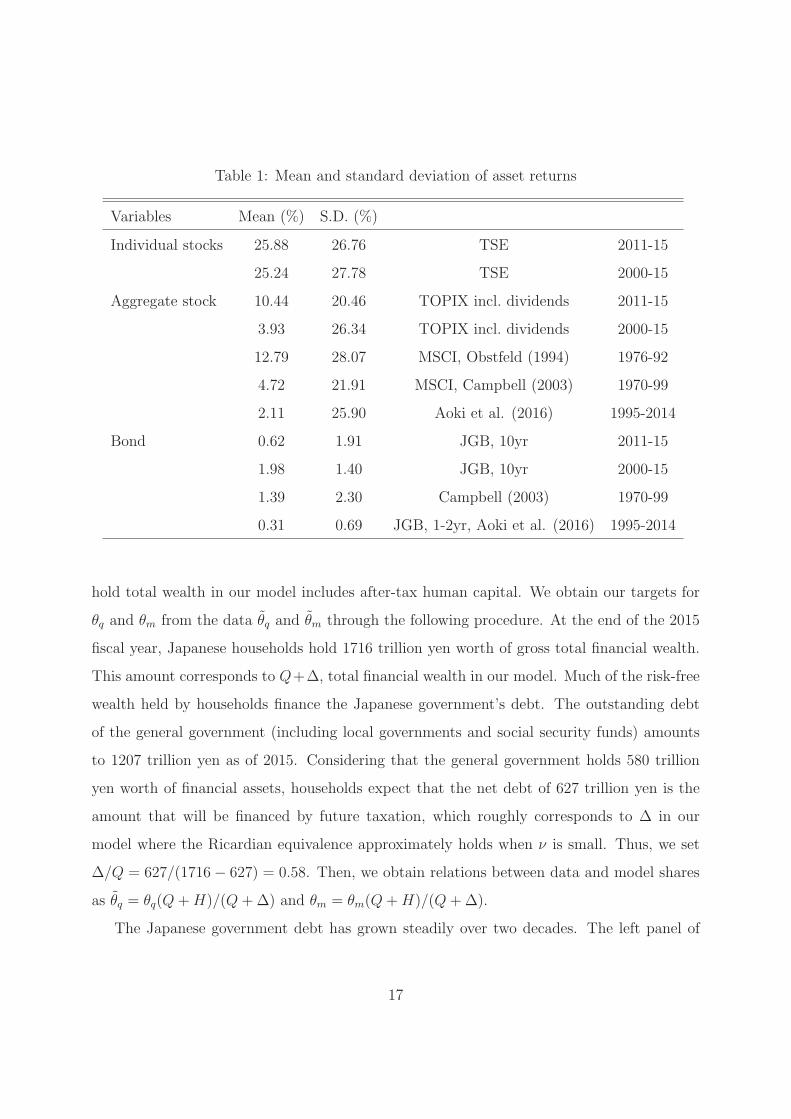
Table 1: Mean and standard deviation of asset returns
Variables Mean (%) S.D. (%)
Individual stocks 25.88 26.76 TSE 2011-15
25.24 27.78 TSE 2000-15
Aggregate stock 10.44 20.46 TOPIX incl. dividends 2011-15
3.93 26.34 TOPIX incl. dividends 2000-15
12.79 28.07 MSCI, Obstfeld (1994) 1976-92
4.72 21.91 MSCI, Campbell (2003) 1970-99
2.11 25.90 Aoki et al. (2016) 1995-2014
Bond 0.62 1.91 JGB, 10yr 2011-15
1.98 1.40 JGB, 10yr 2000-15
1.39 2.30 Campbell (2003) 1970-99
0.31 0.69 JGB, 1-2yr, Aoki et al. (2016) 1995-2014
hold total wealth in our model includes after-tax human capital. We obtain our targets for
θq and θm from the data θq and θm through the following procedure. At the end of the 2015
fiscal year, Japanese households hold 1716 trillion yen worth of gross total financial wealth.
This amount corresponds to Q+Δ, total financial wealth in our model. Much of the risk-free
wealth held by households finance the Japanese government’s debt. The outstanding debt
of the general government (including local governments and social security funds) amounts
to 1207 trillion yen as of 2015. Considering that the general government holds 580 trillion
yen worth of financial assets, households expect that the net debt of 627 trillion yen is the
amount that will be financed by future taxation, which roughly corresponds to Δ in our
model where the Ricardian equivalence approximately holds when ν is small. Thus, we set
Δ/Q = 627/(1716− 627) = 0.58. Then, we obtain relations between data and model shares
as θq = θq(Q+H)/(Q+Δ) and θm = θm(Q+H)/(Q+Δ).
The Japanese government debt has grown steadily over two decades. The left panel of
17

���
���
���
���
���
���� ���� ���� ����
��� ������������ ��� ������������
����
����
��
���
���
���
���� ���� ��� ���
Figure 1: Left: Average return and volatility of individual shares of companies listed on
Tokyo Stock Exchange. Right: Market return of Tokyo Stock Exchange (TOPIX including
dividends). Source: Nikkei Financial Quest.
��
��
��
��
���
���
���
� �� �� ���
��
��
��
��
��
��
�
���� ���� ���� ����
Figure 2: Left: Household portfolio share of equity and stocks θq. Right: Household portfolio
share of mutual funds θm. The shares represent the asset values divided by household total
financial wealth. Source: Flow of Funds, Bank of Japan.
Figure 3 shows the time-series of the net debt of the general government, along with the risk-
free asset holdings of households. We observe that the two time-series grow in tandem, if
not completely parallel. We interpret this relationship in our model as households absorbing
most of the newly issued government bonds by increasing their savings. Thus, an increase
in the government debt holdings by households is cancelled out with a reduction in the
human wealth which reflects increases in future taxation. Since both government debt and
human wealth are risk-free, the household share of risk-free assets is unchanged. This view
of Japanese savings behavior corresponds with that of Hayashi (1986) in which the altruistic
18

Figure 3: Left: Household risk-free assets and government net debt. Source: Flow of Funds
and Ministry of Finance. Right: Pareto exponent of household income. Source: Moriguchi
(2016).
bequest motive plays an important role. Households have a strong incentive to save in our
model of perpetual youth since they face a survival probability independent of age, even
though the Ricardian equivalence does not hold exactly.
In this paper, we do not include housing or mortgage in household net wealth. We instead
treat housing as an imputed consumption included in GDP. Also, we do not consider risky
human capital explicitly. In our model, wealthy households who earn a much larger amount
of business returns from their portfolio θq than their labor income w effectively represent
successful entrepreneurs. Hence, we can view θq as the portfolio allocated to entrepreneurial
endeavor.
For the inequality measure, we use the estimates of the Pareto exponents in Japan pro-
vided by Moriguchi (2016). The average Pareto exponent during 2000-2015 is 2.41. The
Pareto exponent is stationary during this period as seen in the right panel of Figure 3. In
our model, the Pareto exponent of household income coincides with that of wealth. Thus,
we use the estimated value interchangeably for income and wealth.
Other parameter values are calibrated as follows. We choose to set the discount rate ρ
to the standard value of 0.03. We set ν to 0.02, which implies that the average length of a
household is 50 years. In the benchmark model, the coefficient of relative risk aversion γ is
set to 5. This value is used in a DSGE model in Caldara et al. (2012) and is also consistent
19
with the empirical estimate of the Japanese households in the survey data by Ito et al. (2017).
Following Aoki and Nirei (2017), we set φ to 3.33, implying that 30% of firm sales is rent.
The depreciation rate δ is set to 0.089, which is taken from Hayashi and Prescott (2002).
The capital share in GDP, α, is calculated from SNA as 0.3375.
4.2 Benchmark result
In our calibration, we aim to match the mean returns (rf and μm), risks of an individual
stock and a mutual fund (σq and σm), household portfolio shares (θq and θm), and the
Pareto exponent of wealth distribution (λ1). The target moments of portfolio variables are
estimated for the period 2000-2015 as shown in Table 1 except for σq. Table 1 shows that
the individual stock in TSE exhibits very modest volatility that is comparable to the market
volatility during this period. Lacking alternative measurements, we rely on Moskowitz and
Vissing-Jørgensen (2002) for an estimate of volatility of entrepreneurial rate of returns at
0.41 standard deviation. The volatility of mutual funds is set at TSE market volatility, 0.26.
Then, we exploit the model prediction that the ratio of entrepreneurial volatility to market
volatility is scaled as√n, leading to n = 2.43.
Other moments, μm, θq, θm, and λ1, are matched by calibrating four model parameters
related to financial transaction costs: σz, τf , τm, and τp. The riskiness of business is mostly
determined by the size of productivity shock, σz. Thus, we use σz to match σq and μm. The
cost of transformation of risky stocks to risk-free assets, τf , determines the size of overall
risks that households take directly through own business and mutual funds. When τf is high,
households invest less in risk-free assets. The household risk attitude then affects the tail
distribution of wealth and income. The greater the risk-taking, the lower the tail index λ1 and
the less equal the distribution. Hence, λ1 is the main target moment to obtain a calibrated
value for τf . The costs for mutual funds, τm and τp, are used to match the portfolio shares
θm and θq.
Our benchmark parameter values are thus determined as σz = 0.614, τf = 0.123, τm =
0.06, and τp = 0.022. Under these values, we match the target moments as shown in Table
20

2.
Table 2: Calibration targets and endogenous moments
σq μm σm θq θm λ1KY
CY
A−Ha
Yrf
Target 0.411 0.0393 0.2634 0.1057 0.0465 2.41 2.2 0.56 3.3 0.02
Model 0.411 0.0506 0.2712 0.1060 0.0459 2.66 1.8 0.59 4.3 0.04
While it is difficult to find exact empirical counterparts for the transaction costs assumed
in the model, we can evaluate their plausibility by examining the other steady state values
of the model. In particular, τf , τm and τp determine the size of financial costs κ. The model
posits that the portion of goods κ is used to facilitate financial transactions and maturity
transformation from stock shares to deposit. Thus, κ is interpreted as the resources employed
in the financial sector as in Aoki and Nirei (2017). The steady state value for the share of
financial costs in GDP, κ/Y , is 0.068. According to SNA, the share of GDP is 5.2% for the
financial sector and 6.6% for the financial and realty sectors excluding housing. Thus, the
model value matches well with the actual share of the financial sector in Japan.
It is necessary that τf is larger than τm in our model, because otherwise the risky mutual
fund is dominated in its rate of return by the risk-free asset generated by banks. Our
benchmark parameter further assumes that τf is much greater than τm. This corresponds
well with the fact that depository institutions hold large shares in the Japanese financial
industry. The trust and administration fee of mutual funds is represented by τm, which is
charged on the returns of funds in our model. Thus, when the rate of returns of a mutual
fund is 4%, τm = 0.06 which means that 0.24% of fund value is deducted as trust fees. This
value seems plausible for passive index funds purchased by Japanese households. However,
Khorana et al. (2009) reports the trust fees in Japan as 1.25%, which would set our τm
at a higher value 0.31. In addition to τm, our model posits that a household must pay
transaction fees upon the purchase of mutual funds. These fees, as discussed in detail by Cai
et al. (1997), have been historically high in Japan. According to their estimates, upon the
21
purchase of funds during the period between 1981 and 1992, the fees were “typically between
2% and 5% of the investment value”, with a turnover ratio of funds of 110% in 1992. Even
though the purchase costs and the turnover ratio of mutual funds have declined since then,
it is still possible that an annual average rate of this fee, which is represented by τp in our
model, amounts to 2.2% of the invested value as our benchmark calibration assumes.
Under the benchmark parameter values, the model generates steady-state capita-output
ratio K/Y = 1.8, the ratio of household financial wealth to output (A − Ha)/Y = 4.3,
and the consumption-output ratio (ν + ρ)A/Y = 0.59. These ratios at the steady state
roughly match with the corresponding statistics in Japan in 2015, which are 2.2, 3.3, and
0.56, respectively. While the wealth-output ratio is matched well under this calibration with
standard value of time discount rate ρ = 0.03, it is hard to match the observed return of JGB
with our risk-free rate. However, we can match the risk-free rate by setting a low value for
ρ. Our main numerical results continue to hold under the alternative calibration, as shown
in Appendix B.
The low share of mutual funds in household portfolios, at 4.65%, is calibrated in our model
by setting the purchase cost τp high. This is compatible with the low participation rate of
Japanese households in the stock market as documented in Iwaisako (2009) and Fujiki et al.
(2012). The share of mutual funds is remarkably lower than that of U.S. households (Financial
Services Agency, 2016), even though the gap may be overstated due to statistical difference
between two countries (Koike, 2009; Fukuhara, 2016). Kitamura and Uchino (2010) and Ito
et al. (2017) suggest that poor financial literacy is a factor contributing to low participation.
Aoki et al. (2016) and Yamana (2016) provide structural models to gauge the impact of
financial transaction costs in an effort to account for the low participation rate.
4.3 Effects of reduction in financial costs
As we have shown above analytically, a reduction in financial transaction costs encourages
risk-taking, enhances capital accumulation and leads to greater outputs and a lower risk-free
rate, while its impact on inequality is ambiguous. In this section, we investigate the effect of
22
reduced financial costs quantitatively using the benchmark calibrated model. Tables 3 and
4 show the results.
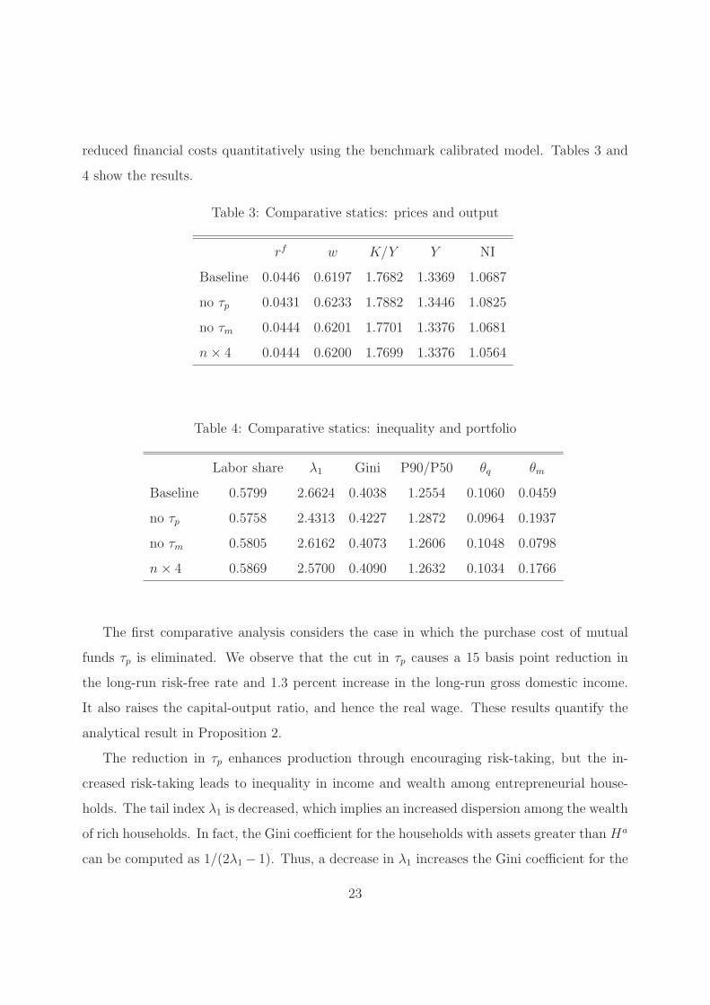
Table 3: Comparative statics: prices and output
rf w K/Y Y NI
Baseline 0.0446 0.6197 1.7682 1.3369 1.0687
no τp 0.0431 0.6233 1.7882 1.3446 1.0825
no τm 0.0444 0.6201 1.7701 1.3376 1.0681
n× 4 0.0444 0.6200 1.7699 1.3376 1.0564
Table 4: Comparative statics: inequality and portfolio
Labor share λ1 Gini P90/P50 θq θm
Baseline 0.5799 2.6624 0.4038 1.2554 0.1060 0.0459
no τp 0.5758 2.4313 0.4227 1.2872 0.0964 0.1937
no τm 0.5805 2.6162 0.4073 1.2606 0.1048 0.0798
n× 4 0.5869 2.5700 0.4090 1.2632 0.1034 0.1766
The first comparative analysis considers the case in which the purchase cost of mutual
funds τp is eliminated. We observe that the cut in τp causes a 15 basis point reduction in
the long-run risk-free rate and 1.3 percent increase in the long-run gross domestic income.
It also raises the capital-output ratio, and hence the real wage. These results quantify the
analytical result in Proposition 2.
The reduction in τp enhances production through encouraging risk-taking, but the in-
creased risk-taking leads to inequality in income and wealth among entrepreneurial house-
holds. The tail index λ1 is decreased, which implies an increased dispersion among the wealth
of rich households. In fact, the Gini coefficient for the households with assets greater than Ha
can be computed as 1/(2λ1 − 1). Thus, a decrease in λ1 increases the Gini coefficient for the
23
wealthy households. We also compute the Gini coefficient of financial wealth for all house-
holds, which is shown in Table 4. The disparity of income between the wealthy households
and the median households is shown by the ratio of wealth between the 90th percentile and
the 50th percentile. The 90/50 disparity increases, because the wealthy households benefit
from the wage increase as much as the median household does.
We conduct similar comparative analyses when τm, the cost of the returns on mutual
funds, is eliminated, and when n, the number of firms included in a mutual fund, is quadrupled
(the magnitude is set so that the effect is comparable with the case τp = 0). An increase
in n diversifies the risk of the mutual funds by a factor of the square root of n. Thus, an
increase in n effectively reduces the cost of risk-bearing through mutual funds, and affects
household portfolio behavior and the steady state similarly as with cuts in transaction costs.
We observe the same responses of the risk-free rate, output, real wage, and most of the
inequality measures qualitatively. An exception is that the labor share of national income
(NI) is increased. This is caused by an increase in capital-output ratio and thus a more-than-
proportional increase in capital depreciation. Households who mainly rely on labor income
certainly gain from the increased capital and thus real wage. The increase in the labor share
is notable for the case of increased n. We did not observe this effect for the elimination of
τp, since an increasing effect on NI due to the reduction of goods used for transaction costs
dominated the effect of the increased capital depreciation in that case.
We conclude this section by discussing whether a reduction of τp and τm may have con-
tributed to the decrease in risk-free rates, given that the banking technology τf has not
changed drastically. The costs τp and τm represent the technology of equity finance, whereas
τf represents the technology of deposit banks. Noting that risky investments suffer infor-
mation asymmetry between creditors and debtors, Greenwood and Jovanovic (1990) argued
that financial intermediation provides not only risk pooling but also research on investment
projects which leads to better allocation of funds and growth. On this ground, Rajan (2005)
warned that the investor incentive problem still remains, even though the world with recent
financial developments has left “the days of bank-dominated systems with limited competi-
tion, risk sharing, and choice.” The Japanese banking sector has maintained a steady level of
24

lending which roughly amounts to the size of Japan’s GDP. In our model, the high share of
risk-free assets of households is upheld by the high costs of participation in the stock markets.
In this setup, a reduction of the participation cost will lead to a shift in the portfolio share
from the risk-free to risky assets. The portfolio shift enhances aggregate capital accumula-
tion, because average intermediation costs are lower in risky assets than in risk-free assets.
As a side effect, the deepening of capital causes a decrease in the risk-free rate. Quantitative
analyses showed that the impact on the risk-free rate is modest at below a percentage point
under the calibration for the Japanese economy. It is left for future research to determine
whether the effect is more pronounced in different environments.
5 Conclusion
This paper quantifies the effect of policies that induce households to shift their portfolios to-
ward business risk-taking. We present a dynamic general equilibrium model with incomplete
markets for business rate-of-return risks. We consider two kinds of financial intermediaries,
banks and mutual funds. Banks transform a continuum of risky equities into a risk-free asset,
which meets household demand for risk-less deposits. Mutual funds pool a finite number of
risky equities and provide risky assets, whose risk is reduced through the diversification of
independent equities. The banks’ transformation services incur relatively high transaction
costs compared to mutual funds, but mutual funds charge an additional cost that is paid
upon purchase of the funds. We posit that households pay an annual rate of purchase costs.
With this setup, we first show analytically that a reduction in transaction costs for mutual
funds increase output and real wage as well as decreasing the risk-free rate in the steady state.
This result is intuitive: the reduction in transaction costs encourages household investments
in risky business projects and results in the accumulation of business capital. The marginal
product of capital decreases as the capital increases, leading to a decline in the risk-free
rate given that banks’ technology is unchanged. Therefore, financial developments favoring
risk-taking result in a decrease in the long-run risk-free rate. Moreover, we derive that
the household wealth follows a double-Pareto distribution in the steady state. The Pareto
25
exponent for the right-tail of the wealth and income distributions is determined by the balance
between the trend growth and the diffusion of individual wealth process. The effect of
reduction in financial transaction costs on wealth dispersion is ambiguous, since the cost
reduction affects both the trend and diffusion of wealth process.
We use the model to quantify the effect of cost reduction in the Japanese economy.
The model is able to reproduce Japanese household portfolios with reasonable calibration of
financial transaction costs. Quantitative analyses show that the reduction in financial costs
result in greater inequality in household financial wealth but may increase the labor share of
gross national income. Quantitative effects of the reduced financial costs are modest overall.
A quantitative analysis under the parameter values calibrated to the Japanese economy
shows that elimination of purchase costs for mutual funds leads to an increase in output by
1.3 percent, a decrease in risk-free rate by 15 basis points, and an increase in Gini coefficient
of wealth in 2 percentage points.
Appendix
A Proofs
Proof of Corollary 1
From the definition of λ1 and ϑ, we observe
∂ϑ
∂μa
=μa
ϑ,
∂ϑ
∂σ2a
=ν
ϑ,
ϑ = λ1σ2a + μa,
ν =ϑ2 − μ2
a
2σ2a
=λ21σ
2a
2+ λ1μa.
26

Using these relations, we obtain that λ1 is decreasing in μa and in σ2a as follows:
∂λ1
∂μa
=1
σ2a
(∂ϑ
∂μa
− 1
)=
1
σ2a
(μa
ϑ− 1
)=
1
σ2a
(μa
λ1σ2a + μa
− 1
)< 0,
∂λ1
∂σ2a
= −λ1
σ2a
+∂ϑ/∂σ2
a
σ2a
=1
σ2a
(νϑ− λ1
)=
1
σ2a
(λ21σ
2a/2 + λ1μa
λ1σ2a + μa
− λ1
)=
1
σ2a
( −λ21σ
2a/2
λ1σ2a + μa
)< 0.
Finally, it is immediate that ∂λ1/∂ν > 0.
Proof of Lemma 1
By modifying Equation (27),
αδ(1− 1/φ)
(1− (ρ+ ν)
1− τfrf
− κ
)− (rf + δ)
(1− (ρ+ ν)
(ϕ(1− τf )
rf+
1− ϕ
rf + ν
)− ϕκ
)= 0.
Taking the total differential of the equation, we obtain
drf[αδ(1− 1/φ)(ρ+ ν)
1− τf(rf )2
−(1− (ρ+ ν)
(ϕ(1− τf )
rf+
1− ϕ
rf + ν
)− ϕκ
)−(rf + δ)(ρ+ ν)
(ϕ(1− τf )
(rf )2+
1− ϕ
(rf + ν)2
)]+ dκ
[−αδ(1− 1/φ) + (rf + δ)ϕ]= 0.
27

This is rewritten as follows.
drf[(ρ+ ν)
1− τf(rf )2
(αδ(1− 1/φ)− (rf + δ)ϕ)−(1− (ρ+ ν)
(ϕ(1− τf )
rf+
1− ϕ
rf + ν
)− ϕκ
)−(rf + δ)(ρ+ ν)
1− ϕ
(rf + ν)2
]+ dκ
[−αδ(1− 1/φ) + (rf + δ)ϕ]= 0.
Now, we have (rf + δ)ϕ/(αδ(1 − 1/φ)) = ϕY/(δK). This is greater than 1, because capital
income net of depreciation cost is positive at the steady state. Thus, (rf + δ)ϕ − (αδ(1 −1/φ)) ≥ 0. Then we obtain that the coefficient for dκ is positive.
A sufficient condition for the coefficient for drf to be negative is
1− (ρ+ ν)
(ϕ(1− τf )
rf+
1− ϕ
rf + ν
)− ϕκ > 0,
which is guaranteed if 1− (ρ+ ν)1−τfrf
−κ > 0 using (27) and Y/(δK) > 0. Hence, under this
condition, the coefficient for drf is negative, and we obtain drf/dκ ≥ 0. In what follows, we
prove that the condition 1− κ > (ρ+ ν)(1− τf )/rf holds for small τp.
By the definition of κ in (26) and D = Qrf/(1− τf ), we obtain
1− κ = 1−(τf − A
Q(θqτf + θm(τf − τm))
)− θmτp
A
Q
1− τfrf
> 1− (τf − (θqτf + θm(τf − τm)))− θmτpA
Q
1− τfrf
= 1− θfτf + θmτm − θmτpA
Q
1− τfrf
(28)
where we use A/Q = 1 +H/Q > 1 in the second line.
The household budget constraint can be aggregated across households at the steady state
as c/a = μa = θqμq + θmμm + θfrf . Substituting policy functions, we obtain
ρ+ ν = θqτfr
f
1− τf+ θm
(τf − τm1− τf
rf − τp
)+ rf .
Rearranging terms gives
(ρ+ ν)(1− τf )/rf = (1− θfτf − θmτm)
ρ+ ν
ρ+ ν + θmτp. (29)
Note that both the right hand sides of (28) and (29) achieve 1− θfτf − θmτf when τp = 0.
Thus, the inequality 1 − κ > (ρ + ν)(1 − τf )/rf holds when τp = 0. Moreover, both sides
of the inequality are continuous in τp. Hence, there exists τp > 0 such that the inequality
1− κ > (ρ+ ν)(1− τf )/rf holds for any τp ∈ (0, τp). �
28

Proof of Proposition 2
We show that κ is increasing in τm and decreasing in rf in Equation (26). First, we modify
(26) using optimal portfolio rules for θ’s as follows:
κ = τf −(θm
(τf − τm − (1− τf )
τprf
)+ θqτf
)(1 +H/Q)
= τf −[n
(τf − τm1− τf
− τp
)(τf − τm − (1− τf )
τprf
)+
τ 2fχ2
1− τf
]rf (1 +H/Q)
γσ2qχ
2(30)
whereH
Q=
rf
rf + ν
(1− α)(1− 1/φ)
1− τf
1
ϕ− αδ(1− 1/φ)/(rf + δ).
We observe that an increase in τm reduces the gap in financial costs τf − τm, and hence
increases κ in (30).
To see the effect of rf on κ in (30), we start by noting that
d
drf[rf (1 +H/Q)
]= 1 +
H
Q
[1 +
d logH/Q
d log rf
].
We want to sign this derivative. Note that
d logH/Q
drf/rf= 1 +
rf
rf + δ− rf
rf + ν− ϕrf
ϕ(rf + δ)− αδ(1− 1/φ).
The sum of the first three terms is positive. The last term plus 1 is positive, since
1− ϕrf
ϕ(rf + δ)− αδ(1− 1/φ)= 1− ϕrf
ϕrf + δ/φ=
δ/φ
ϕrf + δ/φ> 0.
Thus, we obtain (d/drf )(rf (1 +H/Q)) > 0.
In (30), rf affects κ through four factors: −(1−τf )τp/rf , τ 2fχ
2, rf (1+H/Q), and 1/(σ2qχ
2).
We have just shown that the third term is increasing in rf . The fourth term 1/(σ2qχ
2) is also
increasing in rf from (24) and (25). The first and second terms are also increasing in rf .
Since all of these terms contribute to κ negatively, we obtain that κ is decreasing in rf in
(30). From this, we can prove that, when τm increases in (27) and (30), steady state rf must
increase. If we suppose otherwise, then κ in (30) is increased by τm as well as by a decrease
in rf . Then, from the previous lemma, rf must increase in (27). This contradicts with our
premise that rf is decreased. Hence, we prove that rf is increasing in τm.
29

We also note that τp increases κ in (30) while it does not directly affect (27). Proceeding
similarly as in the previous paragraph, we show that rf is increasing in τp.
Finally, κ is decreasing in n in (30) while it does not directly affect (27). Thus, rf is
decreasing in n. �
B Alternative calibration
Under the benchmark calibration, the steady-state risk-free rate is higher than the target
10-year JGB rate. This disparity can be amended by setting the time discount rate ρ to be
as low as 0.005. Also, we reset the risk aversion parameter to γ = 3. With parameter values
set as σz = 0.51, τf = 0.37, τm = 0.05, and τp = 0.014, we can match the target moments as
shown in Table 5.
Table 5: Calibration targets and endogenous moments
σq μm σm θq θm λ1KY
CY
A−Ha
Yrf
Target 0.411 0.0393 0.2634 0.1057 0.0465 2.41 2.2 0.56 3.3 0.0198
Model (main) 0.4110 0.0506 0.2712 0.1060 0.0459 2.66 1.8 0.59 4.3 0.0446
Model (alt.) 0.4075 0.0234 0.2645 0.1047 0.0429 2.67 2.2 0.60 8.6 0.0201
Under these parameter values, the model generates steady-state capita-output ratio at
K/Y = 2.2 and consumption-output ratio at (ν + ρ)A/Y = 0.60. However, the ratio of
household financial wealth to GDP becomes as large as 8.6. The match with the wealth to
GDP ratio is in a trade-off with the match with JGB rate.
The comparative statics with reduced transaction costs are shown in Tables 6 and 7. We
observe that the qualitative patterns of the comparative statics are maintained from the case
with benchmark calibration.
30

Table 6: Comparative statics: prices and output
rf w Y K/Y NI
Baseline 0.0201 0.6869 2.1639 1.4818 1.0952
no τp 0.0194 0.6894 2.1795 1.4872 1.0972
no τm 0.0201 0.6870 2.1646 1.4820 1.0953
n× 4 0.0201 0.6871 2.1651 1.4822 1.0954
Table 7: Comparative statics: inequality and portfolio
Labor share λ1 Gini P90/P50 θq θm
Baseline 2.6667 0.6272 0.4031 1.4810 0.1047 0.0429
no τp 2.4198 0.6283 0.4221 1.5585 0.0915 0.2002
no τm 2.6415 0.6272 0.4051 1.4872 0.1040 0.0635
n× 4 2.6038 0.6273 0.4074 1.4943 0.1029 0.1648
References
Acemoglu, Daron, Philippe Aghion, and Fabrizio Zilibotti, “Distance to frontier, selection,
and economic growth,” Journal of the European Economic Association, 2006, 4, 37–74.
Angeletos, George-Marios and Laurent-Emmanuel Calvet, “Idiosyncratic production risk,
growth and the business cycle,” Journal of Monetary Economics, 2006, 53, 1095–1115.
Aoki, Kosuke, Alexander Michaelides, and Kalin Nikolov, “Household portfolios in a secular
stagnation world: Evidence from Japan,” Bank of Japan Working Paper Series No.16-E-4,
2016.
, Naoko Hara, and Maiko Koga, “Structural reforms, innovation and economic growth,”
Bank of Japan Working Paper Series No.17 E-2, 2017.
31
Aoki, Shuhei and Makoto Nirei, “Zipf’s Law, Pareto’s Law, and the evolution of top incomes
in the United States,” American Economic Journal: Macroeconomics, 2017, 9 (3), 36–71.
Attanasio, Orazio P. and Monica Paiella, “Intertemporal consumption choices, transaction
costs and limited participation in financial markets: Reconciling data and theory,” Journal
of Applied Econometrics, 2011, 26, 322–343.
Benhabib, Jess, Alberto Bisin, and Shenghao Zhu, “The distribution of wealth and fiscal
policy in economies with finitely lived agents,” Econometrica, 2011, 79, 123–157.
Blanchard, Olivier J., “Debt, deficits, and finite horizons,” Journal of Political Economy,
1985, 93 (2), 223–247.
Cai, Jun, K.C. Chan, and Takeshi Yamada, “The performance of Japanese mutual funds,”
Review of Financial Studies, 1997, 10, 237–273.
Caldara, Dario, Jesus Fernandez-Villaverde, Juan F. Rubio-Ramirez, and Wen Yao, “Com-
puting DSGE models with recursive preferences and stochastic volatility,” Review of Eco-
nomic Dynamics, 2012, 15 (2), 188–206.
Campbell, John Y. and Luis M. Viceira, Strategic asset allocation: Portfolio choice for long-
term investors, Oxford University Press, 2002.
Duffie, Darrell and Larry G. Epstein, “Asset pricing with stochastic differential utility,”
Review of Financial Studies, 1992, 5 (3), 411–436.
Financial Services Agency, “Financial Report (in Japanese),” Technical Report, Financial
Services Agency, Japan, 2016.
Fujiki, Hiroshi, Naohisa Hirakata, and Etsuro Shioji, “Aging and household stockholdings:
Evidence from Japanese household survey data,” Institute for Monetary and Economic
Studies Discussion Paper Series, E-17, 2012.
Fukuhara, Toshiyasu, “Nishibei kakei no risuku shisan hoyu ni kansuru ronten seiri,” Bank
of Japan Reports & Research Papers, February 2016.
32
Greenwood, Jeremy and Boyan Jovanovic, “Financial development, growth, and the distri-
bution of income,” Journal of Political Economy, 1990, 98, 1076–1107.
Hayashi, Fumio, “Why is Japan’s saving rate so apparently high?,” NBER Macroeconomics
Annual, 1986.
and Edward C. Prescott, “The 1990s in Japan: A lost decade,” Review of Economic
Dynamics, 2002, 5 (1), 206–235.
Ito, Yuichiro, Yasutaka Takizuka, and Shigeaki Fujiwara, “Kakei no shisan sentaku kodo:
Dogaku paneru bunseki wo mochiita shisan sentaku mekanizumu no kensho,” Bank of
Japan Working Paper Series, No.17-E-6, 2017.
Iwaisako, Tokuo, “Household portfolios in Japan,” Japan and the World Economy, 2009, 21,
373–382.
Jones, Charles I., “Pareto and Piketty: The macroeconomics of top income and wealth
inequality,” Journal of Economic Perspectives, 2015, 29, 29–46.
Khorana, Ajay, Henri Servaes, and Peter Tufano, “Mutual fund fees around the world,”
Review of Financial Studies, 2009, 22, 1279–1310.
Kitamura, Yukinobu and Taisuke Uchino, “Kakei no shisan sentaku kodo ni okeru gakureki
koka: Chikuji kurosu sekushon deta ni yoru jissho bunseki,” Global COE Hi-Stat Discus-
sion Paper Series, Hitotsubashi University, 149, 2010.
Koike, Takuji, “Kakei no hoyu suru risuku shisan: “chochiku kara toshi he” saiko,” Refarensu,
National Diet Library, September 2009.
Moriguchi, Chiaki, “Top income shares and income mobility in Japan,” 2016 LERA Winter
Meetings paper, 2016.
Moskowitz, Tobias J. and Annette Vissing-Jørgensen, “The returns to entrepreneurial invest-
ment: A private equity premium puzzle?,” American Economic Review, 2002, 92, 745–778.
33
Nirei, Makoto and Shuhei Aoki, “Pareto distribution of income in neoclassical growth mod-
els,” Review of Economic Dynamics, 2016, 20, 25–42.
and Wataru Souma, “A two factor model of income distribution dynamics,” Review of
Income and Wealth, 2007, 53 (3), 440–459.
Obstfeld, Maurice, “Risk-taking, global diversification, and growth,” American Economic
Review, December 1994, 84 (5), 1310–1329.
Rajan, Raghuram G., “Has financial development made the world riskier?,” NBER Working
Paper 11728, 2005.
Reed, William J., “The Pareto, Zipf and other power laws,” Economics Letters, 2001, 74,
15–19.
Toda, Alexis Akira, “Incomplete market dynamics and cross-sectional distributions,” Journal
of Economic Theory, 2014, 154, 310–348.
Yaari, Menahem E., “Uncertain lifetime, life insurance, and the theory of the consumer,”
Review of Economic Studies, 1965, 32 (2), 137–150.
Yamana, Kazufumi, “Structural household finance,” Discussion Papers 279, Policy Research
Institute, Ministry of Finance Japan, 2016.
34