ECONOMICS

DETERMINANTS OF INCOME INEQUALITY IN BOTSWANA

by

Zelda Okatch

and

Abu Siddique

and

Anu Rammohan

Business School University of Western Australia

DISCUSSION PAPER 13.15

DETERMINANTS OF INCOME INEQUALITY IN BOTSWANA

by

Zelda Okatch, Abu Siddique and Anu Rammohan

Business School

University of Western Australia

DISCUSSION PAPER 13.15

Abstract

This paper utilizes regression based inequality decomposition methodology developed by

Field (2003) to determine factors driving income inequality at household level in Botswana.

Using the Household Income and Expenditure Survey of 2002/03 an income generating

function is estimated using OLS. This provides an efficient and flexible way to quantify the

roles of household variables like education and age on inequality in a multivariate context.

Results of the inequality decomposition indicate that secondary school education, training,

Value Added Tax, number of children and number of working adults in the household

contribute significantly to inequality in Botswana. On the other hand, variables like primary

education, age and owning between 1 and 10 head of livestock equalises income inequality.

We would like to thank Kazi Iqbal for his invaluable comments on the article.

1. Introduction

Since the discovery of diamonds in the early 1970s, Botswana has experienced phenomenal

growth levels by world standards, with annual growth rates averaging 9% between 1966 and

2002. Growth rates fell to about 7.7% between 2003 and 2006 and have been below 5% in

recent years due to the global financial crisis (Government of Botswana, 2010). Other factors

such as fiscal discipline and sound economic management have also helped Botswana

transform itself from one of the poorest countries in the world to a middle income country

with a per capita GDP of $16,300 in 2011. Poverty has also declined significantly over the

years. The consecutive Household Income Expenditure Surveys (HIES) undertaken in

1985/86, 1993/94, 2002/03 and 2009/10 indicate that the portion of the population living

below the poverty line were 59%, 47%, 30% and 20% respectively. Despite this performance

which could be considered quite remarkable by international comparison, the situation is still

unacceptable to Botswana as growth has not been evenly distributed amongst the population

and inequality levels are relatively high. The HIES data shows that income inequality has

worsened over the 1993/94 to 2002/03 period, with the Gini coefficient of disposable income

increasing from 0.537 to 0.573, respectively.

The high inequality levels could possibly be attributed to the fact that the mineral sector

which drives the economy is highly capital intensive and employs a very small proportion of

the labour force, yet this sector accounts for more than one third of GDP, about 70-80% of

export earnings, and almost half of government revenue. The 2005/06 Botswana Labour

Force Survey indicates that less than 3% of the total labour force was employed by the

mineral sector. However, their average earnings were double the average national rate. The

sector grew by 7.8% between 1991 and 2005 but this was not accompanied by its growth in

employment which remained stagnant during this period. Overall Botswana employment

figures have not lived up to the exceptional economic growth as compared to other middle

income countries employment lags behind. In 2009/10 overall unemployment in Botswana

was estimated at 17.3% by the Botswana Core Welfare Indicator Survey.

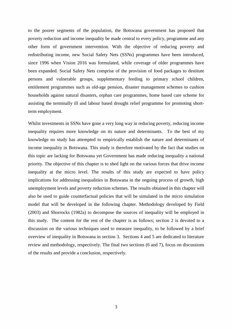
The increasing inequality amidst the impressive economic development can be explained by

Kuznets curves shown in figure 1 below. Kuznets (1955) shows that as development

measured by, per capita income, increases, inequality first worsens then eventually improves.

The explanation of the Kuznets curve pivots on the fact that in preindustrial societies, almost

1

everybody is equally poor so inequality is low. However, inequality will rise as people move

from low productive agriculture to more productive industrial sectors. These industrial

sectors are characterised by higher average income and less uniform wages. As a society

matures and becomes richer, the urban-rural gap is reduced and the provision of old-age

pensions, unemployment benefits, and other social transfers lower inequality. Todora (2011)

establishes three possible scenarios in which growth, measured in GDP per capita, can be

accompanied by an improved income distribution, an unchanged income distribution, or a

case where income distribution worsens. Botswana seems to have experienced the latter

scenario and is in the industrial phase of the Kuznets curve. This can be demonstrated by the

fact that between 1993/94 and 2002/03 real GDP per capita increased from P71541 to

P11802, while income distribution declined in the same period (Bank of Botswana, 2005).

The high inequality level and its increase between 1993/94 and 2002/03, irrespective of the

economic theoretical explanations, is unacceptable according to Botswana’s national

development objectives. The National Development Plan 10 (NDP) covering the period

between 2009/10 and 2016, Vision 2016 and the National Strategy for Poverty Reduction

(NSPR) advocate for eradication of absolute poverty and the significant reduction of income

inequality by 2016. In order to create an environment which permits growth to trickle down

1 P is the symbol for Botswana’s national currency, the Pula. Currently $1 (Australian dollar) is equivalent to P7.5

Gross national income per capita

Gini

Coefficient

Figure 1: The Inverted- U Kuznets Curve

2

to the poorer segments of the population, the Botswana government has proposed that

poverty reduction and income inequality be made central to every policy, programme and any

other form of government intervention. With the objective of reducing poverty and

redistributing income, new Social Safety Nets (SSNs) programmes have been introduced,

since 1996 when Vision 2016 was formulated, while coverage of older programmes have

been expanded. Social Safety Nets comprise of the provision of food packages to destitute

persons and vulnerable groups, supplementary feeding to primary school children,

entitlement programmes such as old-age pension, disaster management schemes to cushion

households against natural disasters, orphan care programmes, home based care scheme for

assisting the terminally ill and labour based drought relief programme for promoting short-

term employment.

Whilst investments in SSNs have gone a very long way in reducing poverty, reducing income

inequality requires more knowledge on its nature and determinants. To the best of my

knowledge no study has attempted to empirically establish the nature and determinants of

income inequality in Botswana. This study is therefore motivated by the fact that studies on

this topic are lacking for Botswana yet Government has made reducing inequality a national

priority. The objective of this chapter is to shed light on the various forces that drive income

inequality at the micro level. The results of this study are expected to have policy

implications for addressing inequalities in Botswana in the ongoing process of growth, high

unemployment levels and poverty reduction schemes. The results obtained in this chapter will

also be used to guide counterfactual policies that will be simulated in the micro simulation

model that will be developed in the following chapter. Methodology developed by Field

(2003) and Shorrocks (1982a) to decompose the sources of inequality will be employed in

this study. The content for the rest of the chapter is as follows; section 2 is devoted to a

discussion on the various techniques used to measure inequality, to be followed by a brief

overview of inequality in Botswana in section 3. Sections 4 and 5 are dedicated to literature

review and methodology, respectively. The final two sections (6 and 7), focus on discussions

of the results and provide a conclusion, respectively.

3

2. Measuring Inequality

Inequality can be considered as a case of different people having different degrees of income

or consumption. Income inequality is mainly concerned with the relative position of different

individuals within the income distribution. It is basically a summary statistic of the income

dispersion. Income distribution can be observed at a personal level or a functional level.

Where the functional distribution of income considers the distribution between groups in

society who own different factors of production, i.e. the proportion of income going to

employees, landowners, and owners of capital respectively. On the other hand, the personal

income distribution is concerned with the national distribution of income without paying too

much attention to the factors of production. This study will focus more on the personal

distribution of income. A number of techniques to measure inequality in a population have

notably been developed and employed over time such as the Gini coefficient, the coefficient

variation of income, the logarithm of income and generalised entropy class of inequality

indices, the Gini coefficient and the Atkinson index. This section will review the desirable

properties of the various inequality measures, discuss a few of these techniques and measures

and subsequently provide some information on decomposition techniques.

2.1 Properties of Inequality Indices

According to Litchfield (1999), economic literature calls for good inequality measures to

satisfy five properties (axioms), namely anonymity, scale independence, population

independence, transfer principle and decomposability. The anonymity axiom requires that an

inequality metric does not depend on the labelling of individuals in an economy and, hence,

concern should be placed only on the distribution of income. This property distinguishes the

concept of inequality from that of fairness. Hence, an inequality measure should not concern

itself with what kind of income certain people deserve, but rather on how it’s distributed. The

scale independence property deals with the fact that the inequality measure should not be

affected by uniform proportional changes in all individuals’ income. For instance if every

person's income in an economy is doubled (or multiplied by any positive constant), then the

overall measure of inequality should not change. The inequality income metric should be

independent of the aggregate level of income.

4

Issues surrounding population independence require that the inequality measure should not be

dependent on the size of the population, such that merging two identical distributions should

not alter inequality. The transfer principle (commonly referred to as the Pigou–Dalton

transfer principle) indicates, in its weak form, that if some income is transferred from a rich

person to a poor person, while still preserving the order of income ranks, then the measured

inequality should not increase. However, in its strong form, the measured level of inequality

should actually decrease.

There should be a coherent relationship between inequality in the whole of society and

inequality in its constituent parts states the decomposability property. For example if

inequality is seen to rise amongst all sub-groups of the population then overall inequality

should also increase. Some measures, such as the Generalised Entropy class of measures, are

easily decomposed and into intuitively appealingly components of within the group

inequality and between the group inequality. In this case total inequality is the sum of the

within the group inequality and between the group inequality. Whereas within the group

inequality refers to the inequality that exists in a particular group of income earners with

certain characteristic, if the average income of all groups were equalized. On the other hand,

between the groups inequality prevails, if all individuals of each population sub-groups have

the mean income of their sub-group (Cowell, 1985).

2.2 Inequality Indices

The Gini coefficient is one of the most widely used measures of inequality and it measures

the extent to which the Lorenz curve departs from the line of equality. It is valued between

zero and one. With zero representing a situation of complete equality, and one a case where

there is absolute inequality. Hence larger values of the Gini represent greater inequality. The

Gini coefficient satisfies the principle of anonymity, scale independence, population

independence and Pigou–Dalton transfer principle. It is widely used across countries and as it

enables easy comparison. It is also available over a series of years and therefore enables

comparisons over periods of time. Despite its advantages, the Gini coefficient, fails the

decomposability axiom in cases where sub-vectors of income overlap. However, there are

ways of decomposing the Gini, but the component terms of total inequality are not always

intuitively or mathematically appealing (Litchfeild, 1999). A generalization of the Gini

5

coefficient, called the extended Gini coefficient, was introduced by Yitzhaki (1983). The new

index accommodates differing aversions to inequality. The Gini Coefficient can be calculated

using the formula in equation 1.

𝐺𝑖𝑛𝑖 = 12 𝑛2𝑦�

∑ ∑ |𝑦𝑖 − 𝑦�|𝑛𝑗

𝑛𝑖=1 (1)

where n is the number of individuals in the sample, 𝑦𝑖 is the income of individual i, 𝑖 ∈

(1, 2, … , 𝑛), and 𝑦� = (1/𝑛) ∑ 𝑦𝑖, the arithmetic mean income.

There are a number of measures of inequality that satisfy all five criteria. Among the most

widely used are the Theil indexes and the mean log deviation measure. Both belong to the

family of generalized entropy inequality measures. Though the Theil index, satisfy all the 5

properties, it has been criticised for lacking a straightforward representation and an appealing

interpretation of the Gini coefficient. Members of the Generalised Entropy (GE) class of

measures have the general formula as follows:

𝐺𝐸(𝛼) = 1𝛼2−𝛼

�1𝑛

∑ �𝑦𝑖𝑦�

�𝛼

𝑛𝑖=1 − 1� (2)

The value of GE ranges from 0 to ∞, with zero representing an equal distribution and higher

values representing higher levels of inequality. The parameter α in the GE class represents the

weight given to distances between incomes at different parts of the income distribution, and

can take any real value. For lower values of α, GE is more sensitive to changes in the lower

tail of the distribution, and for higher values GE is more sensitive to changes that affect the

upper tail. The commonest values of α used are 0, 1 and 2: hence a value of α=0 gives more

weight to distances between incomes in the lower tail, α=1 applies equal weights across the

distribution, while a value of α =2 gives proportionately more weight to gaps in the upper

tail.

Litchfeild (1999) indicates the GE measures with parameters 0 and 1 become two of Theil’s

measures of inequality. The mean log deviation (also known as Theil’s L index) and the Theil

index respectively, are given as follows:

𝐺𝐸(0) = 1𝑛

∑ log 𝑦�𝑦𝑖

𝑛𝑖=1 (3)

𝐺𝐸(1) = 1𝑛

∑ 𝑦𝑖𝑦�

log 𝑦𝑖𝑦�

𝑛𝑖=1 (4)

6

With α = 2 the GE measure becomes 1/2 the squared coefficient of variation, CV:

𝐶𝑉 = 1𝑦�

�1𝑛

∑ (𝑦𝑖 − 𝑦�)2𝑛𝑖=1 �

12� (5)

Other used inequality measure in literature is the Atkinson class of measures. Atkinson’s set

of inequality measures can be decomposed, but the two components of within- and between-

group inequality do not sum to total inequality. It has the general formula given below

𝐴𝜀 = 1 − �1𝑛

∑ �𝑦𝑖𝑦�

�1−𝜀

𝑛𝑖=1 �

1(1−𝜀)�

(6)

Where ε is an inequality aversion parameter and can take values between 0 and infinity. The

higher the value of ε, the more society is concerned about inequality. The Atkinson class of

measures range from 0 to 1, with zero representing no inequality. Setting α =1-ε, the GE class

becomes ordinally equivalent to the Atkinson class, for values of α < 1 (Cowell, 1995).

Another measure of inequality is the Foster-Greer-Thorbecke (sometimes referred to as

FGT). In fact the headcount index, the poverty gap and poverty gap index and the squared

poverty gap index all belong to the Foster-Greer-Thorbecke class of measures using similar

notation. FGT measures the outfall from the poverty line. Therefore it is also considering the

inequality among the poor and it is measured as follows where

𝑃𝛼 = 1𝑛

∑ (𝑧 − 𝑦𝑖 𝑧�𝑞𝑖=1 )𝛼 (𝛼 ≥ 0) (7)

Where z is the poverty line, n is the sample size, q is the number of poor (those with incomes

at or below z), 𝑦𝑖 are individual incomes and α is a sensitivity parameter. If α is low then the

FGT metric weights all the individuals with incomes below z roughly the same. If α is high,

those with the lowest incomes (farthest below z) are given more weight in the measure. The

higher the FGT statistic, the more poverty there is in an economy. If α =0, then the headcount

index is used in the calculation. If we use α=1, we have the poverty gap index being used.

When α =2, then the squared poverty gap index is utilized and this reports both the poverty

and inequality levels among the poor.

Sen Index developed by Sen (1976) takes into consideration the number of poor, the depth of

their poverty, and the distribution of poverty within the group. The index is given by

7

𝑃𝑆 = 𝑃𝑂(1 − (1 − 𝐺𝑃) 𝜇𝑃

𝑍 (8)

where 𝑃𝑂 is the headcount index, 𝜇𝑃 is the mean income (or expenditure) of the poor, and

𝐺𝑃is the Gini coefficient of inequality among the poor.

The Sen Index has the virtue of taking the income distribution among the poor into account.

However the index is almost never used outside of the academic literature as it lacks the

intuitive appeal of some of the simpler measures of poverty. It also cannot be used to

decompose poverty into contributions from different subgroups (Deaton, 1997).

2.3 Inequality Decomposition

Inequality decomposition literature can be traced back to be found in Shorrocks (1980, 1982b

and 1984). In these articles Shorrocks examined decomposition of inequality by income

sources (such as earnings, investment income and transfer payments), by population sub-

groups (such as single persons, married couples, and families with children) and or by sub

aggregates of observations which share common characteristics like age, household size,

region, occupation, or some other attributes. He shows that a broad class of inequality

measures can be decomposed into components reflecting the size, mean and inequality value

of each population sub-group or income source. Generally inequality decomposition is a

standard procedure used to examine the contribution to inequality of particular

characteristics. It can help to shed light on both the structure and dynamics of inequality

(Litchfield 1999). The other pioneer in this field are Bourguignon (1979), Cowell (1980), and

Shorrocks (1982a, 1982b, 1984).Recent literature has gone beyond this and has used

Shorrock’s original decomposition concept, and applied to regression analysis in order to

decompose inequality by explanatory variables. However, regression basis decomposition

will not be discussed in this section but will be tackled in more detail when reviewing the

literature, and in the methodology section. This section will only look at decomposition by

population sub group and by income source.

8

2.3.1 Decomposition by population sub-group.

Decomposition by sub groups allows for the impact of the contribution to overall inequality

of inequality with and between different sub-groups of the population to be accessed. In this

case total inequality in the distribution can be separated into a component of inequality

between the chosen groups (Ib), and the remaining within-group inequality (Iw). This type of

decomposition can only be conducted for one variable at a time. Using this technique total

inequality, I, is decomposed by population subgroups, the Generalised Entropy class can be

expressed as the sum of within-group inequality, Iw, and between group inequality, Ib.

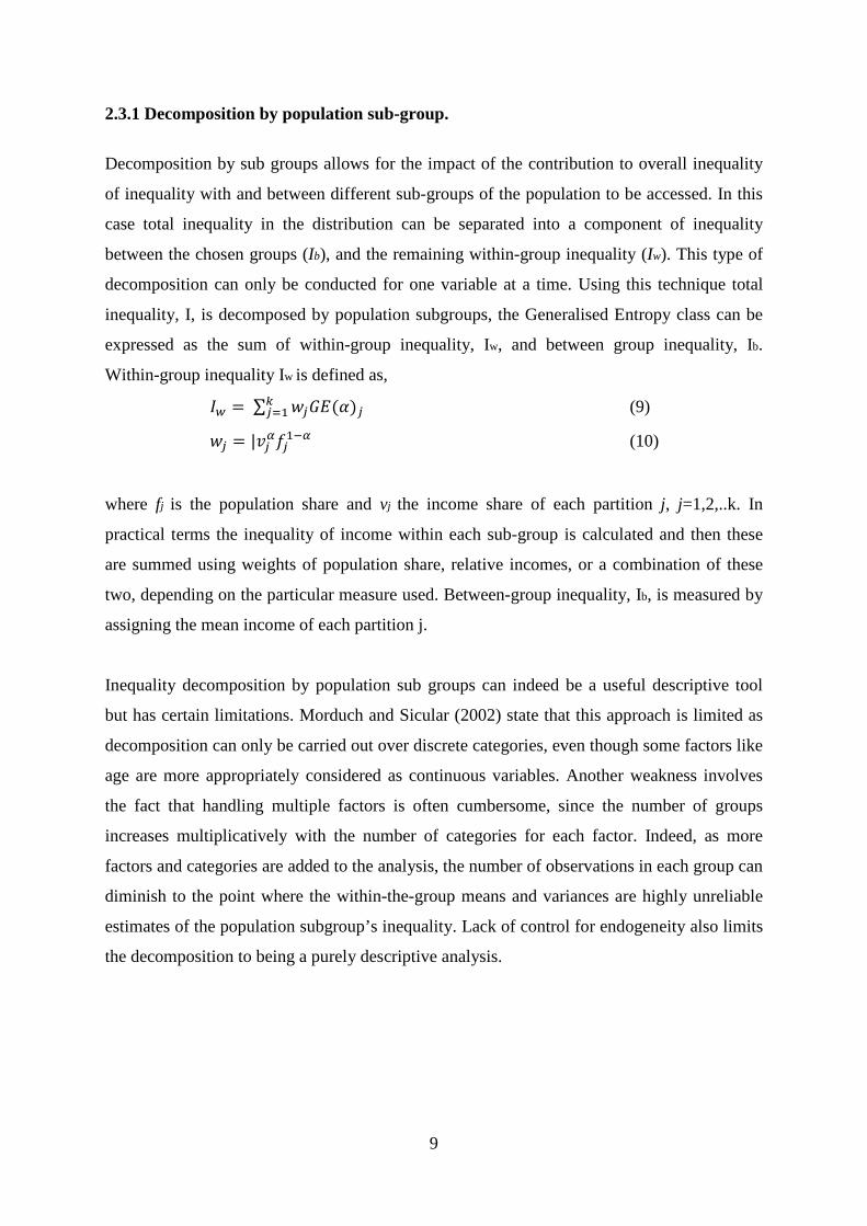
Within-group inequality Iw is defined as,

𝐼𝑤 = ∑ 𝑤𝑗𝐺𝐸(𝛼)𝑗𝑘𝑗=1 (9)

𝑤𝑗 = |𝑣𝑗𝛼𝑓𝑗

1−𝛼 (10)

where fj is the population share and vj the income share of each partition j, j=1,2,..k. In

practical terms the inequality of income within each sub-group is calculated and then these

are summed using weights of population share, relative incomes, or a combination of these

two, depending on the particular measure used. Between-group inequality, Ib, is measured by

assigning the mean income of each partition j.

Inequality decomposition by population sub groups can indeed be a useful descriptive tool

but has certain limitations. Morduch and Sicular (2002) state that this approach is limited as

decomposition can only be carried out over discrete categories, even though some factors like

age are more appropriately considered as continuous variables. Another weakness involves

the fact that handling multiple factors is often cumbersome, since the number of groups

increases multiplicatively with the number of categories for each factor. Indeed, as more

factors and categories are added to the analysis, the number of observations in each group can

diminish to the point where the within-the-group means and variances are highly unreliable

estimates of the population subgroup’s inequality. Lack of control for endogeneity also limits

the decomposition to being a purely descriptive analysis.

9

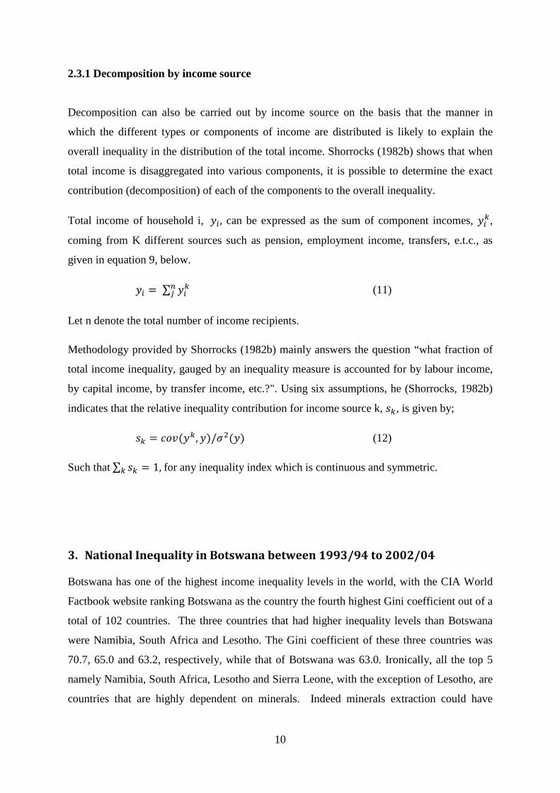
2.3.1 Decomposition by income source

Decomposition can also be carried out by income source on the basis that the manner in

which the different types or components of income are distributed is likely to explain the

overall inequality in the distribution of the total income. Shorrocks (1982b) shows that when

total income is disaggregated into various components, it is possible to determine the exact

contribution (decomposition) of each of the components to the overall inequality.

Total income of household i, 𝑦𝑖, can be expressed as the sum of component incomes, 𝑦𝑖𝑘,

coming from K different sources such as pension, employment income, transfers, e.t.c., as

given in equation 9, below.

𝑦𝑖 = ∑ 𝑦𝑖𝑘𝑛

𝑗 (11)

Let n denote the total number of income recipients.

Methodology provided by Shorrocks (1982b) mainly answers the question “what fraction of

total income inequality, gauged by an inequality measure is accounted for by labour income,

by capital income, by transfer income, etc.?". Using six assumptions, he (Shorrocks, 1982b)

indicates that the relative inequality contribution for income source k, 𝑠𝑘, is given by;

𝑠𝑘 = 𝑐𝑜𝑣(𝑦𝑘, 𝑦)/𝜎2(𝑦) (12)

Such that ∑ 𝑠𝑘 = 1𝑘 , for any inequality index which is continuous and symmetric.

3. National Inequality in Botswana between 1993/94 to 2002/04 Botswana has one of the highest income inequality levels in the world, with the CIA World

Factbook website ranking Botswana as the country the fourth highest Gini coefficient out of a

total of 102 countries. The three countries that had higher inequality levels than Botswana

were Namibia, South Africa and Lesotho. The Gini coefficient of these three countries was

70.7, 65.0 and 63.2, respectively, while that of Botswana was 63.0. Ironically, all the top 5

namely Namibia, South Africa, Lesotho and Sierra Leone, with the exception of Lesotho, are

countries that are highly dependent on minerals. Indeed minerals extraction could have

10

played a significant role in the high levels of inequality because, as stated earlier, they are

capital intensive in nature and relative to its output employment provided by this sector is

limited. While overall employment in Botswana between the 1994/95 and 2002/03 increased

by 23%, employment in the mineral sector only increases by 2%. Yet the output of this sector

more than doubled in real terms.

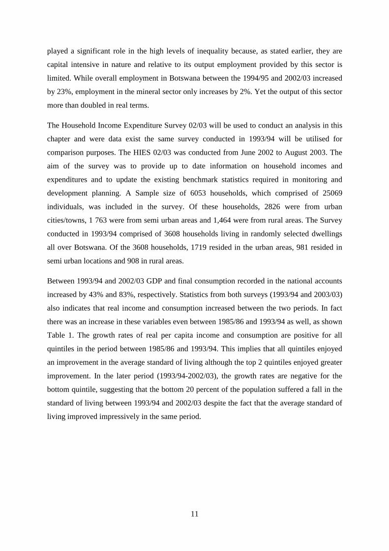
The Household Income Expenditure Survey 02/03 will be used to conduct an analysis in this

chapter and were data exist the same survey conducted in 1993/94 will be utilised for

comparison purposes. The HIES 02/03 was conducted from June 2002 to August 2003. The

aim of the survey was to provide up to date information on household incomes and

expenditures and to update the existing benchmark statistics required in monitoring and

development planning. A Sample size of 6053 households, which comprised of 25069

individuals, was included in the survey. Of these households, 2826 were from urban

cities/towns, 1 763 were from semi urban areas and 1,464 were from rural areas. The Survey

conducted in 1993/94 comprised of 3608 households living in randomly selected dwellings

all over Botswana. Of the 3608 households, 1719 resided in the urban areas, 981 resided in

semi urban locations and 908 in rural areas.

Between 1993/94 and 2002/03 GDP and final consumption recorded in the national accounts

increased by 43% and 83%, respectively. Statistics from both surveys (1993/94 and 2003/03)

also indicates that real income and consumption increased between the two periods. In fact

there was an increase in these variables even between 1985/86 and 1993/94 as well, as shown

Table 1. The growth rates of real per capita income and consumption are positive for all

quintiles in the period between 1985/86 and 1993/94. This implies that all quintiles enjoyed

an improvement in the average standard of living although the top 2 quintiles enjoyed greater

improvement. In the later period (1993/94-2002/03), the growth rates are negative for the

bottom quintile, suggesting that the bottom 20 percent of the population suffered a fall in the

standard of living between 1993/94 and 2002/03 despite the fact that the average standard of

living improved impressively in the same period.

11

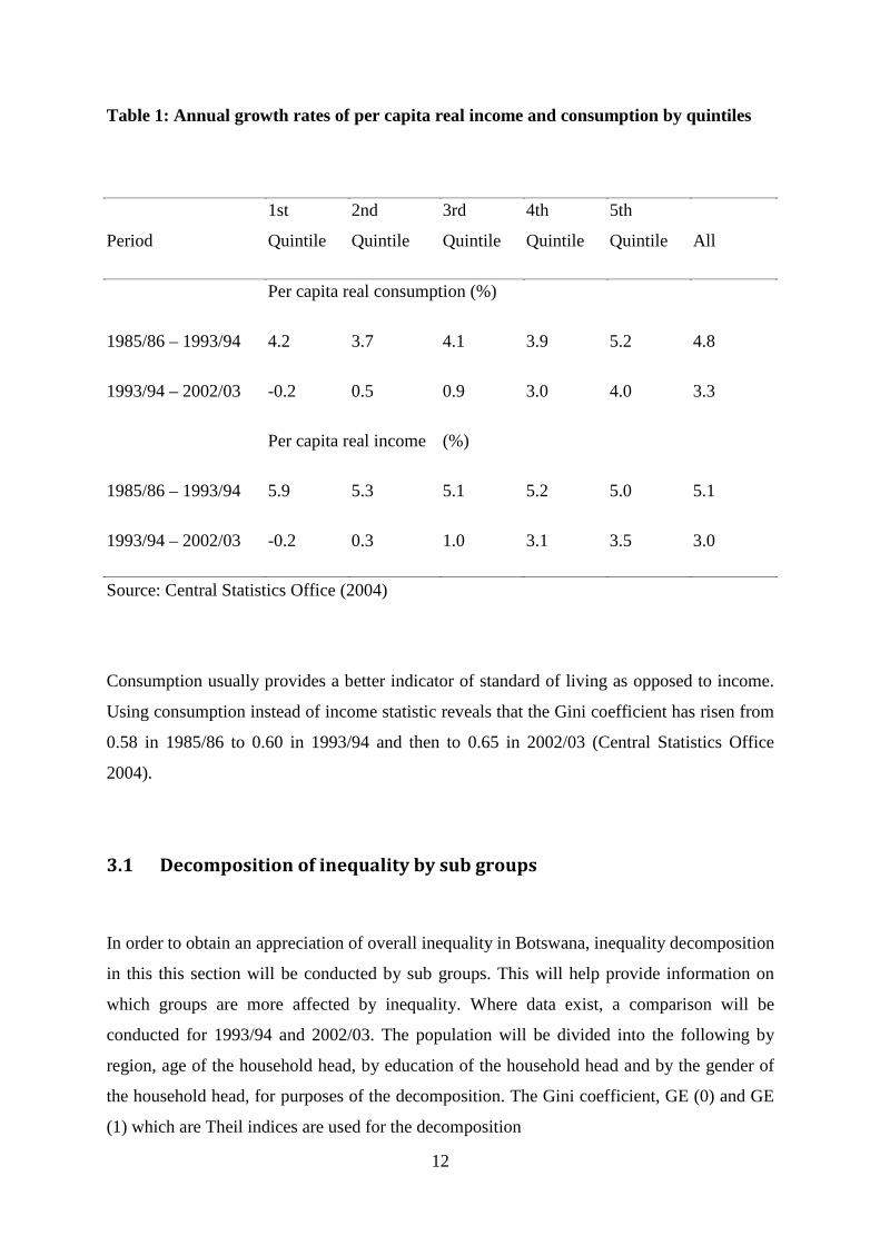
Table 1: Annual growth rates of per capita real income and consumption by quintiles

Period

1st

Quintile

2nd

Quintile

3rd

Quintile

4th

Quintile

5th

Quintile All

Per capita real consumption (%)

1985/86 – 1993/94 4.2 3.7 4.1 3.9 5.2 4.8

1993/94 – 2002/03 -0.2 0.5 0.9 3.0 4.0 3.3

Per capita real income (%)

1985/86 – 1993/94 5.9 5.3 5.1 5.2 5.0 5.1

1993/94 – 2002/03 -0.2 0.3 1.0 3.1 3.5 3.0

Source: Central Statistics Office (2004)

Consumption usually provides a better indicator of standard of living as opposed to income.

Using consumption instead of income statistic reveals that the Gini coefficient has risen from

0.58 in 1985/86 to 0.60 in 1993/94 and then to 0.65 in 2002/03 (Central Statistics Office

2004).

3.1 Decomposition of inequality by sub groups

In order to obtain an appreciation of overall inequality in Botswana, inequality decomposition

in this this section will be conducted by sub groups. This will help provide information on

which groups are more affected by inequality. Where data exist, a comparison will be

conducted for 1993/94 and 2002/03. The population will be divided into the following by

region, age of the household head, by education of the household head and by the gender of

the household head, for purposes of the decomposition. The Gini coefficient, GE (0) and GE

(1) which are Theil indices are used for the decomposition

12

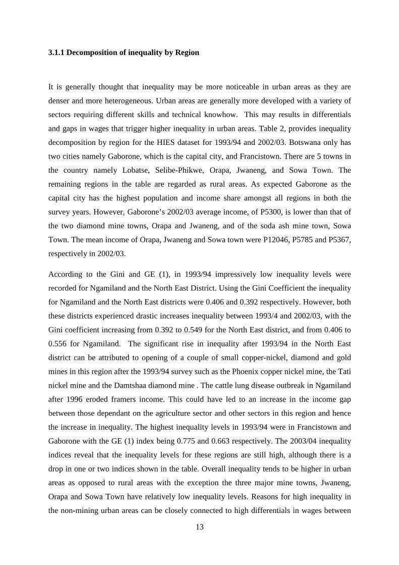
3.1.1 Decomposition of inequality by Region

It is generally thought that inequality may be more noticeable in urban areas as they are

denser and more heterogeneous. Urban areas are generally more developed with a variety of

sectors requiring different skills and technical knowhow. This may results in differentials

and gaps in wages that trigger higher inequality in urban areas. Table 2, provides inequality

decomposition by region for the HIES dataset for 1993/94 and 2002/03. Botswana only has

two cities namely Gaborone, which is the capital city, and Francistown. There are 5 towns in

the country namely Lobatse, Selibe-Phikwe, Orapa, Jwaneng, and Sowa Town. The

remaining regions in the table are regarded as rural areas. As expected Gaborone as the

capital city has the highest population and income share amongst all regions in both the

survey years. However, Gaborone’s 2002/03 average income, of P5300, is lower than that of

the two diamond mine towns, Orapa and Jwaneng, and of the soda ash mine town, Sowa

Town. The mean income of Orapa, Jwaneng and Sowa town were P12046, P5785 and P5367,

respectively in 2002/03.

According to the Gini and GE (1), in 1993/94 impressively low inequality levels were

recorded for Ngamiland and the North East District. Using the Gini Coefficient the inequality

for Ngamiland and the North East districts were 0.406 and 0.392 respectively. However, both

these districts experienced drastic increases inequality between 1993/4 and 2002/03, with the

Gini coefficient increasing from 0.392 to 0.549 for the North East district, and from 0.406 to

0.556 for Ngamiland. The significant rise in inequality after 1993/94 in the North East

district can be attributed to opening of a couple of small copper-nickel, diamond and gold

mines in this region after the 1993/94 survey such as the Phoenix copper nickel mine, the Tati

nickel mine and the Damtshaa diamond mine . The cattle lung disease outbreak in Ngamiland

after 1996 eroded framers income. This could have led to an increase in the income gap

between those dependant on the agriculture sector and other sectors in this region and hence

the increase in inequality. The highest inequality levels in 1993/94 were in Francistown and

Gaborone with the GE (1) index being 0.775 and 0.663 respectively. The 2003/04 inequality

indices reveal that the inequality levels for these regions are still high, although there is a

drop in one or two indices shown in the table. Overall inequality tends to be higher in urban

areas as opposed to rural areas with the exception the three major mine towns, Jwaneng,

Orapa and Sowa Town have relatively low inequality levels. Reasons for high inequality in

the non-mining urban areas can be closely connected to high differentials in wages between

13

those employed and unemployed, and even amongst the employed. The mine towns have

avoided this phenomenon as most of the dwellers in these areas are employed by the mines.

Restriction of entry, by permits, into mine towns such as Orapa discourages migration from

rural areas seeking employment into these towns and therefore keeping inequality relatively

low.

Table 2: Household Inequality Decomposition by Region

Source: Author’s calculation using HIES 1993/94 and 2002/03 dataset

Further decomposition by region is done in Table 3, taking into consideration the level of

development for the 1993/94 and 2002/03 surveys. The three categories under consideration

are urban, semi urban and rural. It’s worth mentioning that the population shares in these

regions have not changed significantly between the two survey periods. However, inequality

using all the three indices has registered a significant decrease for urban villages and rural

areas, inequality in urban areas has also fallen slightly.

HIES 93/94 HIES 02/03

Popn. Share

Mean Income

Income Share

GE(1) Gini Popn Share

Mean Income

Income Share

GE(1) Gini

Gaborone 0.19 2853 0.41 0.663 0.595 0.23 5300 0.38 0.631 0.584

Francistown 0.13 1224 0.12 0.775 0.602 0.1 3914 0.12 0.751 0.615

Lobatse 0.04 1218 0.04 0.496 0.512 0.04 2673 0.03 0.444 0.507

Selibe-Phikwe 0.07 1342 0.07 0.402 0.474 0.07 2676 0.05 0.508 0.521

Orapa 0.01 2308 0.02 0.363 0.463 0.01 12046 0.03 0.328 0.445

Jwaneng 0.03 1826 0.04 0.364 0.47 0.02 5785 0.04 0.448 0.506

Sowa Town 0 5367 0.01 0.155 0.312

Southern districts 0.07 683 0.03 0.537 0.538 0.07 1365 0.03 0.546 0.537

South East District 0.03 928 0.02 0.458 0.504 0.03 3619 0.04 0.62 0.588

Kweneng District 0.1 598 0.04 0.676 0.538 0.09 2039 0.06 0.517 0.527

Kgatleng District 0.03 1033 0.02 0.364 0.451 0.03 2279 0.02 0.525 0.542

Central District 0.22 751 0.12 0.423 0.489 0.21 1874 0.12 0.584 0.569

North East District 0.02 714 0.01 0.287 0.392 0.01 2286 0.01 0.521 0.549

Ngamiland 0.04 809 0.02 0.277 0.406 0.06 2505 0.05 0.549 0.556

Ghanzi 0.02 1046 0.02 0.443 0.516 0.01 3378 0.01 0.334 0.444

Kgalagadi South 0.01 798 0 0.408 0.489 0.01 2109 0.01 0.841 0.642

Within Group 0.57 0.078 0.589 0.263

Between group 0.161 0.306 0.117 0.083

14

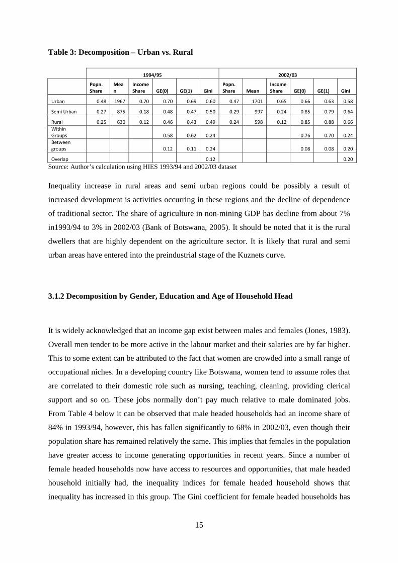
Table 3: Decomposition – Urban vs. Rural

1994/95 2002/03

Popn. Share

Mean

Income Share GE(0) GE(1) Gini

Popn. Share Mean

Income Share GE(0) GE(1) Gini

Urban 0.48 1967 0.70 0.70 0.69 0.60 0.47 1701 0.65 0.66 0.63 0.58

Semi Urban 0.27 875 0.18 0.48 0.47 0.50 0.29 997 0.24 0.85 0.79 0.64

Rural 0.25 630 0.12 0.46 0.43 0.49 0.24 598 0.12 0.85 0.88 0.66 Within Groups 0.58 0.62 0.24 0.76 0.70 0.24 Between groups 0.12 0.11 0.24 0.08 0.08 0.20

Overlap 0.12 0.20 Source: Author’s calculation using HIES 1993/94 and 2002/03 dataset

Inequality increase in rural areas and semi urban regions could be possibly a result of

increased development is activities occurring in these regions and the decline of dependence

of traditional sector. The share of agriculture in non-mining GDP has decline from about 7%

in1993/94 to 3% in 2002/03 (Bank of Botswana, 2005). It should be noted that it is the rural

dwellers that are highly dependent on the agriculture sector. It is likely that rural and semi

urban areas have entered into the preindustrial stage of the Kuznets curve.

3.1.2 Decomposition by Gender, Education and Age of Household Head

It is widely acknowledged that an income gap exist between males and females (Jones, 1983).

Overall men tender to be more active in the labour market and their salaries are by far higher.

This to some extent can be attributed to the fact that women are crowded into a small range of

occupational niches. In a developing country like Botswana, women tend to assume roles that

are correlated to their domestic role such as nursing, teaching, cleaning, providing clerical

support and so on. These jobs normally don’t pay much relative to male dominated jobs.

From Table 4 below it can be observed that male headed households had an income share of

84% in 1993/94, however, this has fallen significantly to 68% in 2002/03, even though their

population share has remained relatively the same. This implies that females in the population

have greater access to income generating opportunities in recent years. Since a number of

female headed households now have access to resources and opportunities, that male headed

household initially had, the inequality indices for female headed household shows that

inequality has increased in this group. The Gini coefficient for female headed households has

15

increased from 0.53 in 1993/94 to 0.63 in 2002/03. All indices also indicate that inequality

within the groups is a greater problem than inequality experienced between the groups.

Generally there seems to be controversy regarding how education affects income inequality.

Education has long been considered a multipurpose policy tool with the main goals

customarily attached to this policy being to lower wage inequality. This connection is

obtained by the fact that education provides skills that can be utilised in the labour market.

Workers with these skills get higher salaries. If more people become educated the income gap

lessens hence inequality declines. This, however, is not always the case. Pereira and Martins

(2004) argue that increasing education attainment could actually lead to higher, not lower,

earnings inequality. This could be a result of poorly designed or out-dated education systems,

where students are provided with skills in large supply and yet there is little demand for those

skills in the labour market. Studies by Mankiw et al (1992) using Slow’s model find a

positive relationship between education and income inequality.

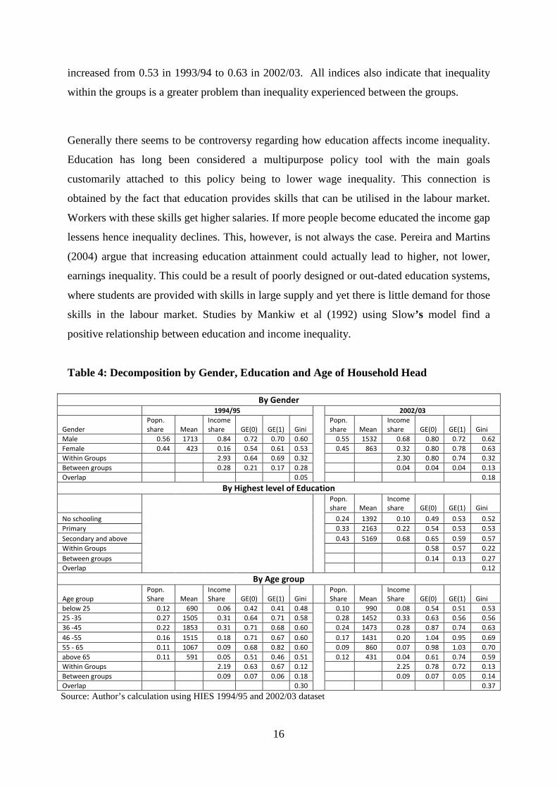
Table 4: Decomposition by Gender, Education and Age of Household Head

Source: Author’s calculation using HIES 1994/95 and 2002/03 dataset

By Gender 1994/95

2002/03

Gender Popn. share Mean

Income share GE(0) GE(1) Gini

Popn. share Mean

Income share GE(0) GE(1) Gini

Male 0.56 1713 0.84 0.72 0.70 0.60 0.55 1532 0.68 0.80 0.72 0.62 Female 0.44 423 0.16 0.54 0.61 0.53 0.45 863 0.32 0.80 0.78 0.63 Within Groups 2.93 0.64 0.69 0.32 2.30 0.80 0.74 0.32 Between groups 0.28 0.21 0.17 0.28 0.04 0.04 0.04 0.13 Overlap 0.05 0.18

By Highest level of Education

Popn. share Mean

Income share GE(0) GE(1) Gini

No schooling

0.24 1392 0.10 0.49 0.53 0.52 Primary

0.33 2163 0.22 0.54 0.53 0.53

Secondary and above

0.43 5169 0.68 0.65 0.59 0.57 Within Groups

0.58 0.57 0.22

Between groups

0.14 0.13 0.27 Overlap

0.12

By Age group

Age group Popn. Share Mean

Income Share GE(0) GE(1) Gini

Popn. Share Mean

Income Share GE(0) GE(1) Gini

below 25 0.12 690 0.06 0.42 0.41 0.48

0.10 990 0.08 0.54 0.51 0.53 25 -35 0.27 1505 0.31 0.64 0.71 0.58 0.28 1452 0.33 0.63 0.56 0.56 36 -45 0.22 1853 0.31 0.71 0.68 0.60 0.24 1473 0.28 0.87 0.74 0.63 46 -55 0.16 1515 0.18 0.71 0.67 0.60 0.17 1431 0.20 1.04 0.95 0.69 55 - 65 0.11 1067 0.09 0.68 0.82 0.60 0.09 860 0.07 0.98 1.03 0.70 above 65 0.11 591 0.05 0.51 0.46 0.51 0.12 431 0.04 0.61 0.74 0.59 Within Groups 2.19 0.63 0.67 0.12 2.25 0.78 0.72 0.13 Between groups 0.09 0.07 0.06 0.18 0.09 0.07 0.05 0.14 Overlap 0.30 0.37

16

From Table 4, it can be observed that inequality is more prevalent in the group with the

highest level of education being secondary school and above. This could be because this

group contains a large number of individuals who have trained further and possess

certificates, diplomas and degrees. These levels of training with in the group create greater

income disparities. There are a number of graduates unable to secure employment due to the

mismatch between the education sector and labour market. This could also explain the high

inequality rate between individual with the highest level of education being secondary school

and above. Decomposition by age of the household indicates that inequality is highest in

groups were household heads are between 36 and 45, 46 and 55, and between 56 and 65 for

both survey periods. These three cohorts have experienced a rise inequality between 1993/94

and 2002/03 with the highest increase being realised in the 55 to 65. Using the Gini

coefficient inequality increased from 0.60 in 1993/94 to 0.70 in 2002/03. In both surveys

inequality is lowest within the lowest and highest cohort. The low inequality levels in

household headed by individuals below 25 could be because this group lacks work

experience that could lead to high dispersion within the group.

3.1.3 Decomposition by Income Factor

As stated earlier, when total income is disaggregated into various components it’s possible to

determine the exact contribution of each component’s overall inequality contribution. Table

5, provides the inequality decomposition by factor components in Botswana using the HIES

1993/1994 and 2002/03 datasets. Note that unearned income includes all payments that

accrue from all factors of production with the exception of wages and business profits. Hence

it includes rent and interest payments. Private transfers include remittances and any other

transfers made by non-public institutes.

17

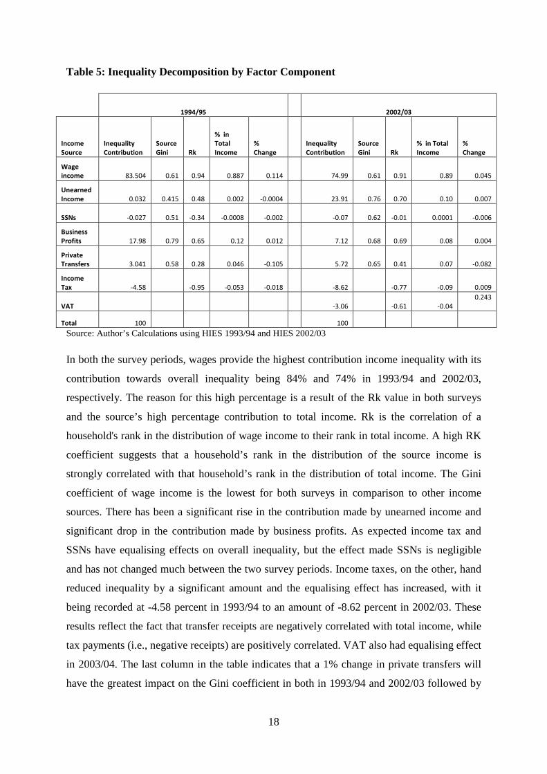
Table 5: Inequality Decomposition by Factor Component

1994/95 2002/03

Income Source

Inequality Contribution

Source Gini Rk

% in Total Income

% Change

Inequality Contribution

Source Gini Rk

% in Total Income

% Change

Wage income 83.504 0.61 0.94 0.887 0.114 74.99 0.61 0.91 0.89 0.045

Unearned Income 0.032 0.415 0.48 0.002 -0.0004 23.91 0.76 0.70 0.10 0.007

SSNs -0.027 0.51 -0.34 -0.0008 -0.002 -0.07 0.62 -0.01 0.0001 -0.006

Business Profits 17.98 0.79 0.65 0.12 0.012 7.12 0.68 0.69 0.08 0.004

Private Transfers 3.041 0.58 0.28 0.046 -0.105 5.72 0.65 0.41 0.07 -0.082

Income Tax -4.58 -0.95 -0.053 -0.018 -8.62 -0.77 -0.09 0.009

VAT -3.06 -0.61 -0.04 0.243

Total 100 100 Source: Author’s Calculations using HIES 1993/94 and HIES 2002/03

In both the survey periods, wages provide the highest contribution income inequality with its

contribution towards overall inequality being 84% and 74% in 1993/94 and 2002/03,

respectively. The reason for this high percentage is a result of the Rk value in both surveys

and the source’s high percentage contribution to total income. Rk is the correlation of a

household's rank in the distribution of wage income to their rank in total income. A high RK

coefficient suggests that a household’s rank in the distribution of the source income is

strongly correlated with that household’s rank in the distribution of total income. The Gini

coefficient of wage income is the lowest for both surveys in comparison to other income

sources. There has been a significant rise in the contribution made by unearned income and

significant drop in the contribution made by business profits. As expected income tax and

SSNs have equalising effects on overall inequality, but the effect made SSNs is negligible

and has not changed much between the two survey periods. Income taxes, on the other, hand

reduced inequality by a significant amount and the equalising effect has increased, with it

being recorded at -4.58 percent in 1993/94 to an amount of -8.62 percent in 2002/03. These

results reflect the fact that transfer receipts are negatively correlated with total income, while

tax payments (i.e., negative receipts) are positively correlated. VAT also had equalising effect

in 2003/04. The last column in the table indicates that a 1% change in private transfers will

have the greatest impact on the Gini coefficient in both in 1993/94 and 2002/03 followed by

18

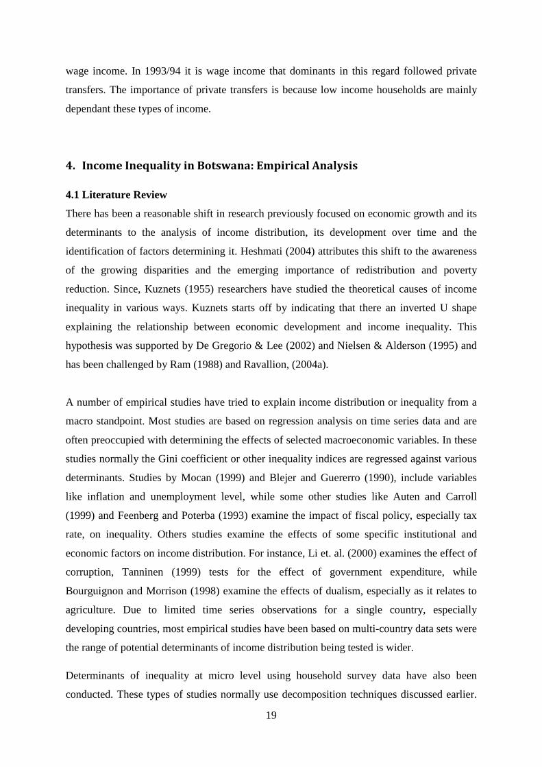
wage income. In 1993/94 it is wage income that dominants in this regard followed private

transfers. The importance of private transfers is because low income households are mainly

dependant these types of income.

4. Income Inequality in Botswana: Empirical Analysis

4.1 Literature Review

There has been a reasonable shift in research previously focused on economic growth and its

determinants to the analysis of income distribution, its development over time and the

identification of factors determining it. Heshmati (2004) attributes this shift to the awareness

of the growing disparities and the emerging importance of redistribution and poverty

reduction. Since, Kuznets (1955) researchers have studied the theoretical causes of income

inequality in various ways. Kuznets starts off by indicating that there an inverted U shape

explaining the relationship between economic development and income inequality. This

hypothesis was supported by De Gregorio & Lee (2002) and Nielsen & Alderson (1995) and

has been challenged by Ram (1988) and Ravallion, (2004a).

A number of empirical studies have tried to explain income distribution or inequality from a

macro standpoint. Most studies are based on regression analysis on time series data and are

often preoccupied with determining the effects of selected macroeconomic variables. In these

studies normally the Gini coefficient or other inequality indices are regressed against various

determinants. Studies by Mocan (1999) and Blejer and Guererro (1990), include variables

like inflation and unemployment level, while some other studies like Auten and Carroll

(1999) and Feenberg and Poterba (1993) examine the impact of fiscal policy, especially tax

rate, on inequality. Others studies examine the effects of some specific institutional and

economic factors on income distribution. For instance, Li et. al. (2000) examines the effect of

corruption, Tanninen (1999) tests for the effect of government expenditure, while

Bourguignon and Morrison (1998) examine the effects of dualism, especially as it relates to

agriculture. Due to limited time series observations for a single country, especially

developing countries, most empirical studies have been based on multi-country data sets were

the range of potential determinants of income distribution being tested is wider.

Determinants of inequality at micro level using household survey data have also been

conducted. These types of studies normally use decomposition techniques discussed earlier.

19

Decomposition by population group has been the oldest approach for quantifying how

various factors affects overall inequality. The approach begins by dividing a sample into

discrete categories (eg, rural and urban residents, individuals with primary school vs.

secondary or higher education) and then calculates the level of inequality within each sub-

sample and between the means of the sub-samples. This technique is mainly conducted in

unpublished articles and a few published articles such as Silber (1989) Jenkins (1995),

Cowell and Jenkins (1995) and Shorrocks (1983).

A second type of inequality decomposition commonly used in literature focuses on the

decomposition by factor components. Shorrocks (1983) uses data on the distribution of net

family incomes in the United States between 1968 and 1977 in order to establish what

proportion of total income inequality is attributable to various income sources using a variety

of different decomposition rules. Decomposition was carried for the following income

sources; wage earnings, capital income, transfer income, and taxes. The findings from this

study showed that labour income had the largest amount of inequality contribution followed

capital earnings. Tax payments and transfers income generate negative contributions in all

years. Results from these types of studies can sometimes have conflicting results depending

on the region. For instance income from non-farming activities was found to have an

equalizing effect in the following studies by El-Osta et al. (1995) for the United States, Zhu

and Luo (2006) for China, Adams (2001) for Egypt and Leones and Feldman (1998) for the

Philippines. On the other hand, Elbers and Lanjouw (2001) found that income from non-

farming contributed positively to inequality for Ecuador. On the contrary, Canagarajah et. al.

(2001) found that in Ghana and Uganda, non-farm self-employment income was much more

disequalizing than non-farm wages.

Regression based estimates in inequality analysis are relatively new and dates back to Oaxaca

(1973). Regression-based approaches to inequality decomposition are appealing because they

overcome many of the limitations of standard decomposition by groups and it’s built on

techniques used by inequality factor decomposition. Using Regression based analysis allows

the use of continuous variables and it is possible to control for endogeneity (Morduch &

Sicualar, 2002). Potential influences on inequality that might require separate modelling, as

in the case of decomposition by groups or by income components, can be easily and

uniformly incorporated within the same econometric model by appropriate specification of

the explanatory variables (Cowell and Fioro, 2009).

20

Morduch & Sicualar (2002) noted that earlier work on regression-based methods of

inequality has been piece-meal, with each proposed approach having different properties and

using different inequality indices. They use a regression-based income inequality

decomposition approach on rural data on china over a period of four years in order examine

how different decomposition rules affect the decomposition results. Findings from Morduch

and Sicular's work vary enormously with the different inequality decomposition indices

giving different results. The Theil-T decomposition shows that human capital and

demographic variables have been strongly inequality reducing. On the other hand, the Gini

decomposition indicates that these variables contribute positively, although modestly, to

inequality. The authors concluded that the Theil-T decomposition provides a better indicator.

Field (2003) presents a methodology to account for income inequality levels in a given

country and differences in income inequality between one time period and another. This

technique is then applied to the US using survey for two time periods, 1979 and 1999, to

analyse labour earnings inequality. The technique starts off by estimating a semi-logarithmic

income generating , using OLS, which included the following variables, gender, industry,

occupation, education, race, region and experience. Field (2003) further demonstrates the

relative factor inequality weights and the corresponding percentage contributions would be

virtually the same for any inequality measure used. The study finds that schooling is the

variable that contributes most to high levels of inequality followed by occupation, experience,

and gender. In explaining the increase in inequality between the two time periods (1979 and

1999), schooling was again the single most important variable followed by occupation.

Gender worked in the equalizing direction.

Cowell and Fioro (2009) uses some features of Field’s (2003) model and extends it by

including the analysis the decomposition by subgroups. This technique is applied to survey

data for Finland and the United States for 1986 and 2004, respectively. The regression based

results for the United States indicated that Master/PhD qualification and age provided the

highest contributions to inequality, while high school education provided an equalising effect.

On the other hand, in Finland a college degree and the number of earners in the household

were more important. High school education in Finland also provided an equalising effect for

Finland.

Wan and Zhou (2005) combine the regression-based decomposition technique and the

Shapley value framework developed Shorrocks (1999) in analysing income inequality in rural

21

China between 1996 and 2002. The decomposition of income inequality is provided by the

Theil –L and the Gini coefficient. The study finds that geographical conditions are the most

significant contributor followed by capital input. The only equalizing variable is land input

but its impact is minimal. Baye and Epo (2011), apply the regression-based inequality

decomposition approach to explore determinants of income inequality in Cameroon using the

2007 Cameroon household consumption survey. They use also Shapley value decomposition

rule to conduct the decompositions and also use a control function approach that tests for

potential endogeneity and unobserved heterogeneity of synthetic variables for education and

health. The results of this study indicate that education is the main contributor to inequality.

Bourgguignon et al. (2001) adopt a simultaneous-equation extension of the Blinder-Oaxaca

decomposition technique. The model estimates an earnings equation (linking individual

characteristics to their remuneration, also known as the occupation effect), a labour supply

equation (explaining the decision of entering the labour force depending on individual and

other household’s members decisions, also known as the participation effect) and a household

income equation (aggregating the individual’s contributions to household income formation

also, known as the population effect). Micro simulation techniques are then used to combine

these equations and decompose inequality by each effect. This study finds that between

1979 and 1994, inequality in Taiwan can mainly be explained by the drastic transformation in

the economy and the socio demographic structure of the population. With the main

contribution being changes in the wage structure which could have been a result a dramatic

growth of the educated workers in the economy. Bourguigion et al. (2008) also use this

technique to isolate the occupational effect, the participation effect and population effect for

USA and Brazil in1999. Results of this study show that most of Brazil’s inequality (of 13

Gini points) is accounted for by underlying inequalities in the distributions of education and

of non-labor income, notably pensions. Differences in occupational structure, in racial

earnings and demographic composition are much less important. While the US the latter are

of more importance.

22

4.2 Contributions

Although numerous empirical studies have been conducted on the subject, most of these have

focused on developed countries and a few developing countries. Due to limited income

distribution data on African, very few studies have been conducted to determine drivers of

income distribution for African countries. And although African countries have been included

in studies that use panel data, the number of African countries covered often constitutes a

negligible fraction of the total. Currently there is no record of any study conducted on

Botswana. This study will fill the gap that exist in literature and examine the subject from a

Botswana perspective. This highly necessary as the government of Botswana has declared

fighting poverty and inequality its priority.

4.3 Methodology

This study will use Field’s (2003) regression based decomposition technique to establish the

determinants of inequality in Botswana. Field (2003) extends Shorrocks' theorem and applies

it to an income-generating function in order to account for or decompose the level of income

inequality contributed by explanatory variables in a country and its change over time. This is

possible as the income generating function has the same additive form as equation 11, which

expresses total income as the sum of the income from various components.

The standard income generating function written in the following form;

𝑙𝑛𝑦𝑖 == 𝑎′𝑍𝑖 (13a)

Where

𝑎 = [𝛼 𝛽1 𝛽2 … 𝛽𝑗 1] (13b)

And

𝑍𝑖 = [1 𝑥𝑖1 𝑥𝑖2 … 𝑥𝑖𝑗 ∈𝑖] (13c)

23

Where, ln𝑦𝑖 is a vector of household income in log, Z is an matrix of household

characteristics (such as age, education, household size, residence, including the residual), 𝑎 is

a vector of the regression coefficients.

Equation 13a will be estimated using OLS and its parameters can be used to calculate the log

of income represented in equation 14.

𝑙𝑛𝑦 = ∑ 𝑎𝑗𝑍𝑗𝑗+2𝑗 (14)

Note that the equation 14 has the same additive form as equation 11, with 𝑦𝑖𝑘replacing 𝑎𝑗𝑍𝑗

and y replacing lny. Now, taking advantage of this homeomorphism and applying Shorrocks

theorem, we take the covariance of both sides of equation 14. Since the left-hand side of 14 is

the covariance between lny and itself, it is simply the variance of lny. Thus,

𝜎2(𝑙𝑛𝑦) = ∑ 𝑐𝑜𝑣 [𝑎𝑗𝑍𝑗 , 𝑙𝑛𝑦]𝑗+2𝑗=1 (15a)

Dividing both sides by 𝜎2(𝑙𝑛𝑦), we obtain

100% = ∑ 𝑐𝑜𝑣 [𝑎𝑗𝑍𝑗,𝑙𝑛𝑦]𝑗+2

𝑗=1

𝜎2(𝑙𝑛𝑦) ≡ ∑ 𝑆𝑗(𝑙𝑛𝑦)𝑗+2𝑗 (15b)

Where, each 𝑠𝑗(𝑙𝑛𝑦) is a so-called "relative factor inequality weight" given by

𝑠𝑗(𝑙𝑛𝑦) = 𝑐𝑜𝑣�𝑎𝑗𝑍𝑗 , 𝑙𝑛𝑦�/𝜎2(𝑙𝑛𝑦) (15c)

let 𝑠𝑗(𝑙𝑛𝑦) denote the share of the log-variance of income that is attributable to the j'th

explanatory factor and let 𝑅2(𝑙𝑛𝑦) be the fraction of the log-variance that is explained by all

of the Z's taken together. Then the below follows;

∑ 𝑠𝑗𝑗+2𝑗=1 (𝑙𝑛𝑦) = 100% (15d)

And

∑ 𝑠𝑗𝑗+2𝑗=1 (𝑙𝑛𝑦) = 𝑅2(𝑙𝑛𝑦) (15e)

The fraction that is explained by the j'th explanatory factor, 𝑝𝑖(𝑙𝑛𝑦) is then

24

𝑝𝑖(𝑙𝑛𝑦) ≡ 𝑠𝑗(𝑙𝑛𝑦)𝑅2(𝑙𝑛𝑦)

(15f)

Note that equation 13c shows the relative factor inequality weight of explanatory variable j

and it’s very similar to equation 10 used by Shorrocks (1982a) to decompose inequality by

income source k. In equation 13c the product of the OLS coefficient and explanatory

variable is regarded as the income flow associated with the explanatory variable. Therefore

this product is what is decomposed to obtain the inequality contribution of an explanatory

variable.

4.4 Econometric Model, Data Description and Empirical Results

4.3.1 The model

As discussed, this study uses Field (2003)’s model to establish to explain the determinants of

inequality in Botswana using the 2002/2003 Household Income Expenditure Survey.

According to Gindling and Trejos (2007), Field’s decompositions have important advantages

over other recently-developed regression-based techniques to measure ‘quantity’ and ‘price’

effects such as those of Bourguignon, Fournier and Gurgand (2001). The latter

decompositions use simulation techniques, such that decompositions of the change in

inequality between two years are based on simulations which start with the distribution for

year one and then substitute (one at a time) the distribution and price of each characteristic

from year two into the earnings equation for year one, measuring the change in inequality in

the resulting distribution of earnings in each case. The change in inequality in the simulated

distributions resulting from changing the price and quantity of each variable is then

interpreted as the contribution of that price or quantity to the change in inequality. A

limitation of these simulation-based techniques is that the results of these simulations will be

different depending on the order in which the variables are substituted, a problem that

Bourguignon, et. al. (2001) calls path dependence. Therefore, the researcher cannot be sure of

the contribution of each variable to the change in inequality unless the results from all

possible ‘paths’ are calculated (and are of similar signs and magnitudes). Calculating the

distributions using every possible path becomes cumbersome especially if the number of

variables to be considered is large.

In addition to the constraints outlined above, Field’s technique is used in the study as it

allows for decomposition to be done even when only one survey period is available. This is

25

very important as the 1994/1995 Household income survey has limited variables and hence

the Bourguignon et. al.’s (2001) technique cannot be employed. Model specification is

mainly guided by previous studies on income inequality and on the available variables in the

Household Income Expenditure Survey. As the first step of the regression-based

decomposition, an income-generation function must be obtained. The income function below

is employed to decompose household inequality by contributing factors.

𝑰𝒏𝒀𝒊 = ∑ 𝜷𝒋 ∗ 𝑿𝒊𝒋 + 𝝐𝒊 (16)

Where 𝐼𝑛𝑌𝑖 is the log of monthly income per capita for household i, 𝑋𝑖𝑗 are variables j

associated with household i that affect income and 𝜖𝑖 is the residual term which can be

explained as the part of the variation in income among workers that cannot be captured by

variation in the variables included in the earnings equation. The use of the semi-log

specification is prompted by the finding that the income variable can be approximated well

by a log-normal distribution (Shorrocks and Wan, 2004).

The right-hand-side variables included in 𝑋𝑖𝑗, whether the household head has a primary

education (PRISCH), whether the household head has a secondary education (SECSCH),

whether the household head has some form of training and possesses a certificate, a diploma,

or a university degree (TRIAN), age of the household head (AGE), age of the household head

squared (AGESQ), number of cattle owned by the household (CATTLE), the amount VAT

paid by the household (VAT), the whether the household receives social safety nets (SSN ), a

dummy variable to capture whether the household resides in an urban area (URB), a dummy

variable capturing whether the household head is male (MALE), number of persons

employed in the household (WORK), number of children in the household (KID). Also

included in the regression are dummy variables that equal one if workers belong to one of

three industries. The industries included are the public sector (GOVT), mining (MIN), and

agriculture (AGRIC), with all the other sectors being used as a reference sector.

4.3.2 Data and Descriptive Statistics

The study uses the Household Income and Expenditure Survey (HIES) of 2002/03, which, as

stated earlier covered 6 053 households, which contained a total of 23 823 individuals. From

the 6 053 households, 2 826 were from the urban areas, 1 763 were from urban villages and

26

the remaining 1 464 were from rural areas. The descriptive statistics of the variable used are

provided in Table 6.

Murduch and Sicular (2002) state that income sources or variables that contribute positively

to total income and are relatively distributed evenly with in the population or mainly

available to the poorer segments of the population, then decomposition will registers

substantial inequality reductions. On the other hand, variables or income sources that

contribute negatively and are distributed relatively evenly will show substantial inequality

increases. Hence the contribution to inequality of a variable is not only dependant on its

relation to income but also on its distribution amongst the population. As indicated earlier

the descriptive statistic for each variable and the distribution of the variable by quartile of

income is provided in Table 6. However, in some case the distribution of the variable and its

impact on income alone may not be sufficient to explain its impact on inequality as other

factor may also come in play. For instance education is normally found to have a positive

relationship with income but even in cases where education is evenly distributed amongst the

population the overall impact on inequality could be positive. This could occur in cases

where there is a mismatch between the labour market and education systems.

From Table 6, it can be observed that household with higher income tend to have household

heads that have a secondary school qualification and are trained. Household heads of high

income household also tend to be employed in the mining or government sector and have

more household members actively engaged in the labour force. On the other hand, it is

observed that households in the lower quartile tend to have more children and older

household heads. While variables that are skewed towards low income households are no of

children, age of the household head, whether household head is engaged in the agriculture

sector, SSNs and primary school education. This implies that low income households on

average tend to have more children, tend to have household heads who involved in the

agriculture sector and rely more on SSNs. Households heads in the lower quartile also tend to

have primary school education as the highest level of education attained and have older

household heads. This could be the case because older household heads lived their younger

years at a time when education was only available to the privileged few. It was only in the

80’s that education was made free for all by the government. Changes in the age structure are

one of the most important factors affecting income inequality trends especially in the long

term (Karunaratne, 2000). In the human capital theory age is normally used as a means to

27

capture the level of experiences as it is expected that the older one becomes the more

experience they acquire. As such an increase in age would lead to an increase in income but

this may fall after the retirement age. Hence age squared is included in the regression in order

to account for the non-linearity of the variable.

Cattle ownership is an increasing category variable which captures the number of cattle

owned. A categorical variable is used instead of the number of cattle owned as this is how the

variable is presented in the dataset. A clear breakdown of the varies categories of this variable

is provided in Table 6. In Botswana, cattle are very important and considered a symbol of

wealth and measure of assets owned. It owed by both low income and high income

households alike as shown in table 6. Although asset can be used instead of cattle in the

African context this variable is very important and can used to obtain a higher standard of

living as it provides milk and can be used for ploughing purposes.

Social safety nets, the urban dummy and the male dummy are all expected to have a positive

relationship in the income function. Generally social safety nets are expected to have an

equalising effect on income inequality especially since populations in higher deciles have less

access. Urban residency may have either an equalising effect or have a positive impact on

inequality. This sign is mainly dependant of the availability of employment, the market size

and the general development level and not only on its distribution level. The male dummy is

expected to have a positive effect on inequality as male headed households have higher

income levels, higher education levels and they normally possess larger amount of assets.

The number of workers is a variable to capture the number of household members who are

engaged in paid activities. The more workers a household has the greater the income the

household will receive. Its contribution to inequality is expected to be high.

28

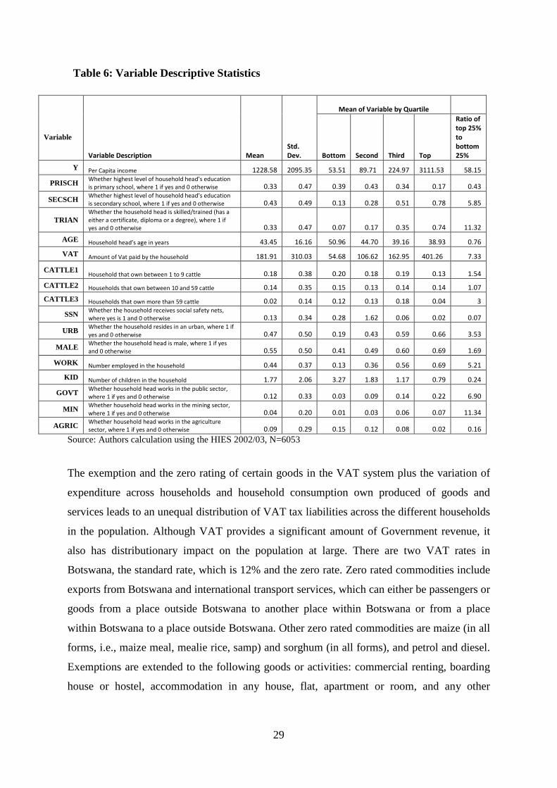
Table 6: Variable Descriptive Statistics

Mean of Variable by Quartile

Variable

Variable Description Mean Std. Dev. Bottom Second Third Top

Ratio of top 25% to bottom 25%

Y Per Capita income 1228.58 2095.35 53.51 89.71 224.97 3111.53 58.15

PRISCH Whether highest level of household head’s education is primary school, where 1 if yes and 0 otherwise 0.33 0.47 0.39 0.43 0.34 0.17 0.43

SECSCH Whether highest level of household head’s education is secondary school, where 1 if yes and 0 otherwise 0.43 0.49 0.13 0.28 0.51 0.78 5.85

TRIAN Whether the household head is skilled/trained (has a either a certificate, diploma or a degree), where 1 if yes and 0 otherwise 0.33 0.47 0.07 0.17 0.35 0.74 11.32

AGE Household head’s age in years 43.45 16.16 50.96 44.70 39.16 38.93 0.76

VAT Amount of Vat paid by the household 181.91 310.03 54.68 106.62 162.95 401.26 7.33

CATTLE1 Household that own between 1 to 9 cattle 0.18 0.38 0.20 0.18 0.19 0.13 1.54

CATTLE2 Households that own between 10 and 59 cattle 0.14 0.35 0.15 0.13 0.14 0.14 1.07 CATTLE3 Households that own more than 59 cattle 0.02 0.14 0.12 0.13 0.18 0.04 3

SSN Whether the household receives social safety nets, where yes is 1 and 0 otherwise 0.13 0.34 0.28 1.62 0.06 0.02 0.07

URB Whether the household resides in an urban, where 1 if yes and 0 otherwise 0.47 0.50 0.19 0.43 0.59 0.66 3.53

MALE Whether the household head is male, where 1 if yes and 0 otherwise 0.55 0.50 0.41 0.49 0.60 0.69 1.69

WORK Number employed in the household 0.44 0.37 0.13 0.36 0.56 0.69 5.21

KID Number of children in the household 1.77 2.06 3.27 1.83 1.17 0.79 0.24

GOVT Whether household head works in the public sector, where 1 if yes and 0 otherwise 0.12 0.33 0.03 0.09 0.14 0.22 6.90

MIN Whether household head works in the mining sector, where 1 if yes and 0 otherwise 0.04 0.20 0.01 0.03 0.06 0.07 11.34

AGRIC Whether household head works in the agriculture sector, where 1 if yes and 0 otherwise 0.09 0.29 0.15 0.12 0.08 0.02 0.16

Source: Authors calculation using the HIES 2002/03, N=6053

The exemption and the zero rating of certain goods in the VAT system plus the variation of

expenditure across households and household consumption own produced of goods and

services leads to an unequal distribution of VAT tax liabilities across the different households

in the population. Although VAT provides a significant amount of Government revenue, it

also has distributionary impact on the population at large. There are two VAT rates in

Botswana, the standard rate, which is 12% and the zero rate. Zero rated commodities include

exports from Botswana and international transport services, which can either be passengers or

goods from a place outside Botswana to another place within Botswana or from a place

within Botswana to a place outside Botswana. Other zero rated commodities are maize (in all

forms, i.e., maize meal, mealie rice, samp) and sorghum (in all forms), and petrol and diesel.

Exemptions are extended to the following goods or activities: commercial renting, boarding

house or hostel, accommodation in any house, flat, apartment or room, and any other

29

accommodation. Other exempted goods include international financial services, education

and specified drugs, as indicated in the Drugs and Related Substances Act. As indicated in

The HIES dataset provides information on 432 goods and services purchased by the

household as well as the value of consumption of goods and services produced by the

household. Given this information VAT paid by each household is estimated from the

household’s expenditure on various goods and services. The estimation ignores the fact that

VAT is not paid goods purchased from small businesses that have an annual sales of less than

P250 000. This is because the size of the informal sector in Botswana is small (Central

Statistic Office,2007).

Pearson Correlation test, shown in Table 7 below, was conducted to establish the pair-wise

relationship between variables. The table shows that most of the pair-wise correlation

relationships are relatively low with the exception of the correlations between AGE and

AGESQ. The results suggest that multicollinearity is not a serious factor in the model.

30

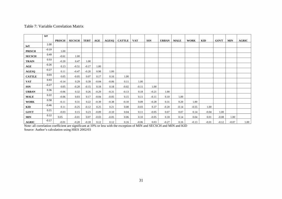
Table 7: Variable Correlation Matrix

lnY

PRISCH SECSCH TERT AGE AGESQ CATTLE VAT SSN URBAN MALE WORK KID GOVT MIN AGRIC

lnY 1.00

PRISCH -0.19 1.00

SECSCH 0.49 -0.61 1.00

TRAIN 0.53 -0.20 0.47 1.00

AGE -0.26 0.13 -0.51 -0.17 1.00

AGESQ -0.27 0.11 -0.47 -0.20 0.98 1.00

CATTLE 0.03 0.05 -0.05 0.07 0.17 0.16 1.00

VAT 0.43 -0.14 0.29 0.39 -0.04 -0.06 0.11 1.00

SSN -0.27 0.05 -0.20 -0.15 0.18 0.18 -0.02 -0.11 1.00

URBAN 0.36 -0.06 0.32 0.26 -0.29 -0.31 -0.13 0.18 -0.21 1.00

MALE 0.22 -0.06 0.03 0.17 -0.04 -0.05 0.15 0.11 -0.11 0.10 1.00

WORK 0.58 -0.11 0.31 0.22 -0.39 -0.38 -0.10 0.09 -0.28 0.31 0.20 1.00

KID -0.46 0.11 -0.25 -0.12 0.25 0.21 0.08 -0.03 0.37 -0.20 -0.14 -0.55 1.00

GOVT 0.21 -0.03 0.15 0.23 -0.09 -0.10 0.04 0.11 -0.05 0.07 0.07 0.14 -0.04 1.00

MIN 0.12 0.05 -0.01 0.07 -0.03 -0.05 0.06 0.10 -0.05 0.18 0.14 0.04 0.01 -0.08 1.00

AGRIC -0.17 -0.01 -0.20 -0.18 0.12 0.12 0.16 -0.06 0.03 -0.27 0.16 -0.13 -0.01 -0.12 -0.07 1.00 Note: all correlation coefficient are significant at 10% or less with the exception of MIN and SECSCH and MIN and KID Source: Author’s calculation using HIES 2002/03

31

4.3.1 Empirical Results

The OLS results of the income function and the inequality decomposition for each variable

using the 2002/03 HIES is given in Table 7. Two specifications are run. The first

specification excludes VAT and SSNs while the second includes them. The inclusion of VAT

and SSNs requires justification as these variables are likely to be correlated to dependant

variable (per capita household income). However, the correlation coefficients presented in 7

shows that correlation between these variables and income are acceptable. The use of a

dummy variable to capture SSNs and categorical variable to capture VAT removes most of

the causality effect between these variables and income. The two variables could not be

excluded as they are important parts of the study. The results of the income function and

variable contribution to inequality of specification 1 are provided in column 2 and 3,

respectively, of Table 7. While that of specification 2 are given in column 4 and 5. An

increase in all variables with the exception of age squared, number of children and the

agriculture dummy have a positive impact on income in both regressions. As stated earlier,

generally low income household have more children, tend to be engaged in the agriculture

sector and have older household heads and, thus, explaining the negative relationship. If

evenly distributed, variables that have a positive impact on income should contribute

negatively to inequality as stated by Morduch and Sicular (2002). All variables in both

income regressions are statistically significant at 1% and has the expected sign with the

exception of SSN and CATTLE 1. SSN could be insignificant as most SSNs programs are not

means tested and are received by a low portion of the population. And even the average

amount received by these households is very low (an equivalent of 27 Australian dollars per

month).

The two education variables, PRISCH and SECSCH, and the training variable, TRAIN, have

the expected sign and are statistically significant. Of these three variables, secondary

education has the greatest impact on income such that obtaining a secondary school

qualification increases ones income by close to 70%. Having a secondary school

qualification increases ones income so greatly and widens the income gap in the population.

Due to this secondary education provided the second largest contribution to inequality, with

this contribution being 15.55% in the first specification and 12.30% in the second

specification. Primary schooling, on the

32

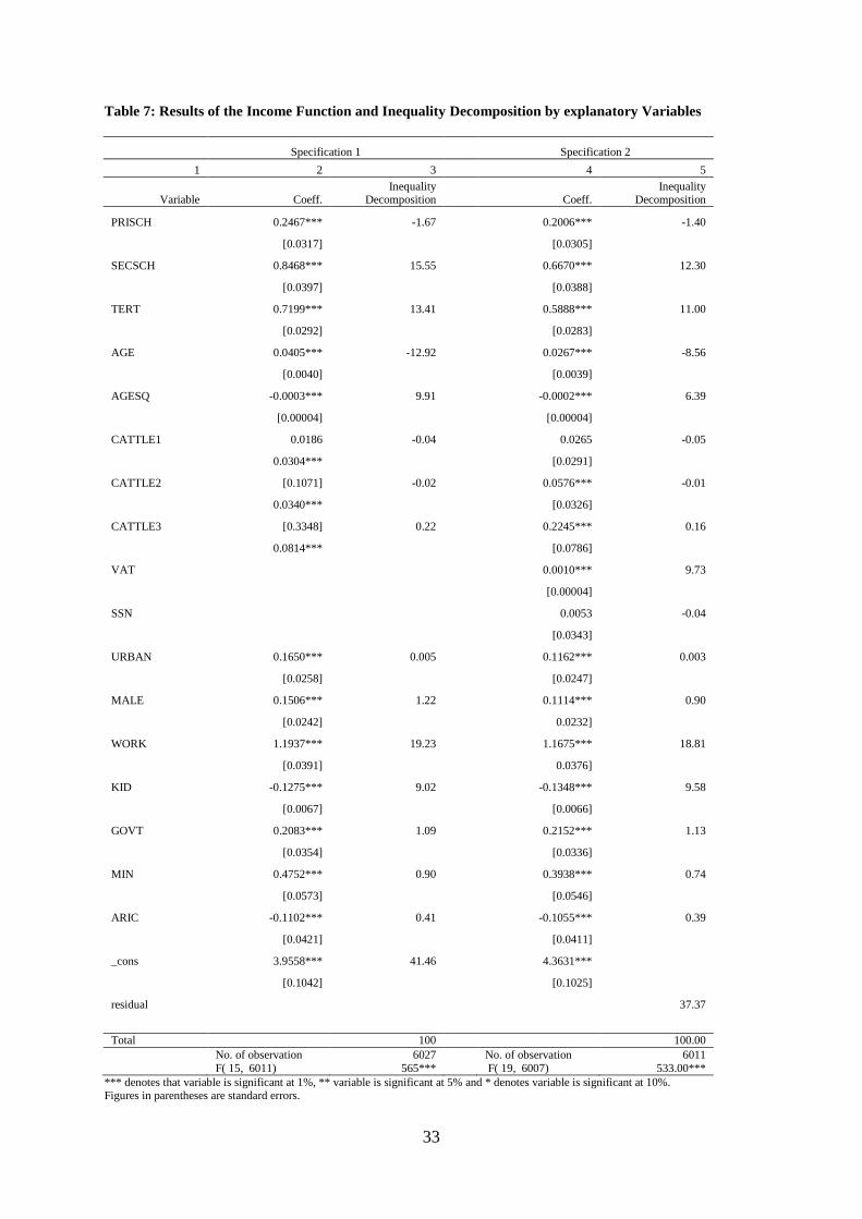
Table 7: Results of the Income Function and Inequality Decomposition by explanatory Variables

Specification 1 Specification 2 1 2 3 4 5

Variable Coeff. Inequality

Decomposition

Coeff. Inequality

Decomposition

PRISCH 0.2467*** -1.67

0.2006*** -1.40

[0.0317]

[0.0305]

SECSCH 0.8468*** 15.55

0.6670*** 12.30

[0.0397]

[0.0388]

TERT 0.7199*** 13.41

0.5888*** 11.00

[0.0292]

[0.0283]

AGE 0.0405*** -12.92

0.0267*** -8.56

[0.0040]

[0.0039]

AGESQ -0.0003*** 9.91

-0.0002*** 6.39

[0.00004]

[0.00004]

CATTLE1 0.0186 -0.04

0.0265 -0.05

0.0304***

[0.0291]

CATTLE2 [0.1071] -0.02

0.0576*** -0.01

0.0340***

[0.0326]

CATTLE3 [0.3348] 0.22

0.2245*** 0.16

0.0814***

[0.0786]

VAT

0.0010*** 9.73

[0.00004]

SSN

0.0053 -0.04

[0.0343]

URBAN 0.1650*** 0.005

0.1162*** 0.003

[0.0258]

[0.0247]

MALE 0.1506*** 1.22

0.1114*** 0.90

[0.0242]

0.0232]

WORK 1.1937*** 19.23

1.1675*** 18.81

[0.0391]

0.0376]

KID -0.1275*** 9.02

-0.1348*** 9.58

[0.0067]

[0.0066]

GOVT 0.2083*** 1.09

0.2152*** 1.13

[0.0354]

[0.0336]

MIN 0.4752*** 0.90

0.3938*** 0.74

[0.0573]

[0.0546]

ARIC -0.1102*** 0.41

-0.1055*** 0.39

[0.0421]

[0.0411]

_cons 3.9558*** 41.46

4.3631***

[0.1042]

[0.1025]

residual

37.37

Total 100 100.00 No. of observation 6027 No. of observation 6011 F( 15, 6011) 565*** F( 19, 6007) 533.00***

*** denotes that variable is significant at 1%, ** variable is significant at 5% and * denotes variable is significant at 10%. Figures in parentheses are standard errors.

33

other hand, has an equalising effect on income in reference to household heads that have no

formal education. However, this equalising effect is very small with its contribution to

inequality being -1.67 and -1.40 in specifications 1 and 2, respectively. The equalising effect

of primary school is derived from not only from the fact that the variable is distributed in

favour of low income households but also from the fact that primary education enables

households to engage in more income generating opportunities compared to their non-

educated counterparts. More opportunities are available to individuals with primary education

as most employers in Botswana prefer individuals who are literate and able to speak English

even for non-skilled jobs. Training also contributed both positively and significantly towards

inequality in both income regressions. These results are consistent with previous studies

using the regression based inequality decomposition such as studies by Baye and Ngah

(2011) for Cameroon, Cowel and Carlo (2009) for Finland, and Wan and Zho (2005). The

contribution of secondary school is higher than that of the training variable by about 2%. The

training contribution to inequality could be affected by the mismatch between the education

sector and the skills required in the labour market as explained by Pereira and Martins (2004).

This is a major concern in Botswana and its intensity has been outlined by Siphambe (2008),

Bolaane et al (2010), and the Botswana’s government National Human Resource

Development Strategy.

Age of the household head has a positive sign, while age squared has a negative sign. Both

these variables are significant and correctly signed as postulated by the human capital theory,

showing that income increases with age, but at a decreasing rate. The overall contribution to

inequality by age and age squared combined is -3.01% and -2.17% for the specification 1 and

2, respectively. This result shows that age equalises income inequality. Besides the fact that

age is distributed towards low income households, a factor that could explain why age is

associated with lower inequality could be that with age comes greater wisdom, knowledge

and experience that improves the ability to generate income and improve the quality life of

even of poor households.

Increasing the number of paid workers in a household by one unit would lead to an increase

of household income. This variable contributes the largest to inequality with the contribution

being 19.3% and 18.81% for specification 1 and 2, respectively. Generally it appears that

higher income households have a larger proportion of paid employees working relative to low

income households. In both regressions the more children one has the less income is

acquired. This could be due to the fact that the more kids could potentially reduce the ability

34

to engage in the labour market as more time is required for child care. The number of

children leads to an increase in inequality. The decomposition of inequality contribution is

given by the number of children is 9.02% and 9.58% in specifications 1 and 2, respectively.

In reference to such as services and manufacturing, working in the agriculture sector leads to

a fall income. While working in the mining sector will lead to an increase in income by 39%.

The various sector contributions to inequality are mainly negligible with government

providing the largest contribution to inequality followed by mining. Although more low

income household ate engaged in agriculture, this variable doesn’t equalise income. This

could be attributed to the low returns to agriculture as only 7% of Botswana soils are suitable

for crop production. The low contribution of mining employment to overall inequality is

shocking especially since this variable is highly distributed in favour of high income

households. The male and the urban residency variables also provide a small but positive

contribution to inequality. In reference to having no cattle households having between 1 to 9

and 10 to 60 cattle provide an equalising effect to inequality, while households with more

than 60 cattle contribute positively, although negligible, to inequality.

VAT, in regression 1, is positively related to income showing that higher levels of VAT paid

is associated with higher incomes. Similar results were obtained by BIDPA (2005). VAT

provides a 9.73% contribution to inequality. Yet VAT payment is relatively fairly distributed

amongst the population with Table 6 indicating that ratio of the top 25% to that of bottom

25% is 1.57. Further calculations actually indicate that households in lower deciles pay a

slightly lower effect VAT rate than households in higher deciles. With household in the

lowest deciles paying an effective VAT rate of 6.25%, while households in the highest decile

have an effective VAT rate of 6.89%. So although high income household pay higher amount

of money for VAT their effective VAT rate is not much different relatively to poorer

households. This is because most of the goods that are zero rated or exempted are goods

consumed by the fairly well off such as education, petrol and diesel and air travel to

destination outside the country. With regards to education, low income households use the

public education system which is free and hence this doesn’t count as part of their

expenditure while high income households utilise the private education which counts as part

of their expenditure. Yet this aspect is VAT exempt and this lowers their overall effective

VAT rate for richer households. All food except for the staple food, maize and sorghum,

have a rate of 12% yet food consumption accounts for 69% of household expenditure in the

lowest decile. While top decile’s expenditure on food is less than 10%.

35

Decomposition of inequality reveals that about 41.46% and 37.37% of inequality in

specification 1 and 2, respectively, is derived from the residual term. This residual

contribution captures attributes in inequality that are not captured by regression. It captures

the unobserved effects on inequality such as the effects of variables like economic growth

and trade liberalisation. Though this value may seem high, it is consistent with other studies.

In fact most studies have found relatively higher contributions of the residual term to

inequality. For instance, Morduch and Sicular have an error term contribution of as high as

90% when decomposition was carried out using Theil’s index. The contribution falls to 40%

when the Gini coefficient is used. Although they concluded that Theil’s index provided a

better measure. Wan and Zhou (2005) run a number of regression for a couple of surveys

conducted in different years and their highest residual contribution to inequality is recorded at

40%. Yun (2006) finds the contribution of the residual to be as high as 78.3%.

Conclusion and Policy Recommendation

In order to summarise these finding, the explanatory variables can be divided into three

groups. With the first group comprising of variables that contribute significantly to income

inequality. These variables are secondary school education, training, VAT and number of

paid employees and number of children in the household. The second group comprises of

variable that have a positive but a small impacts on inequality such as all the sector dummies,

the urban dummy, the male dummy and cattle ownership above 60 cattle. While the third

group comprises of variables that equalises income such as primary education, age, cattle

ownership below 59 cattle and social safety nets.

Policy recommendations is that attempts should be made to reduce the effects on inequality

of the first group while increase the impact or effects of the third group. Under the last group

the only variable that could effective used to lower inequality is primary education. Although

quality free primary and secondary education is provided by government, this education is

not compulsory. Therefore, it is recommended that Government make education compulsory

at both primary and secondary level. Providing free education for all and making it

compulsory would boost the effects of both primary and secondary education on inequality.

This is particularly the case as its low income households that have a higher proportion of

members who have no education. Therefore increase education to this group at primary level

would increasing the equalising effect of primary education and decrease the impact of the

36

positive inequality contribution of secondary school education. There is, however, a need to

increase the number of schools if education is to be made compulsory. Under age the

payment amount of old age pension could be should be reviewed. Other social safety nets

schemes should also be reviewed in order to improve overall their effectiveness. This is

highly important as the sole objective of these programs is to reduce poverty and income

inequality.

With respect to variables in the first group, like training and paid employment, it is important

to embark on policies that will increase the spread and access of these variables to low

income households. Botswana should also consider a child benefit scheme for poor

household as it is currently done in South Africa. However this should be carefully designed

so as not encourage low household to have more children. An income tax policy could also

be introduced that takes into consideration the number of children a household has. VAT on

goods heavily consumed by low incomes households, like food items, should be either zero

rated or exempted. While VAT should be imposed or increased on goods heavily consumed

by high income households. In the following chapter these recommendations will be taken on

board and counterfactual tax and benefit policies will be designed and simulated in a micro

simulation model in order to observe their overall impact on inequality and poverty.

37

5. References Adams, Richard H Jr. (2001). ‘Nonfarm Income, Inequality, and Land in Rural Egypt,’

Economic Development and Cultural Change, vol. 50, pp 339-363.

Atkinson, AB (1970), ‘On the Measurement of Inequality,’ Journal of Economic Theory,

vol. 2, pp. 244-263.

Atkinson, A.B (1983), The Economics of Inequality, Clarendon Press, II ed. Oxford, UK.

Auten, G & Carroll, F (1999), ‘The Effects of Income Taxes on Household Income’, Review

of Economics and Statistics, vol. 81, no. 4, pp. 681–93.

Bank of Botswana, (2005), Botswana Financial Statistics

Baye, Francis Menjo and Epo, Boniface Ngah (2011) “Inequality Decomposition by

Regressed-Income Sources in Cameroon” Prepared for the Special IARIW-SSA Conference

on Measuring National Income, Wealth, Poverty, and Inequality in African Countries Cape

Town, South Africa, September 28-October 1, 2011

BIDPA (2005), Consultancy on Poverty Simulations, Submitted to WIDER

BIDPA (2006), Consultancy on the Review of Social Safety Nets, Submitted to the

Government of Botswana

Blejer, MI & Guerrero, I(1990), ‘The Impact of Macroeconomic Policies on Income

Distribution: An Empirical Study of Philippines’, Review of Economics and Statistics, vol.

72, pp. 414–23.

Bolaane, Benjamin., Chuma, Joseph M., Toteng, Bogadi., & Molwane, O.B. (2010), Tracer

study on the Employment outcome of the Vocational Training Graduates, Consultancy

conducted for the Botswana Training Authority (BOTA)

Bourguignon, F. (1979), ‘Decomposable Income Inequality Measures’, Econometrica, vol.

47, pp. 901-20.

Bourguignon, F., Ferreira, FHG., & Leite, PG, (2008), ‘Beyond Oaxaca-Blinder: Accounting for differences in household income distributions’, Journal of Economic Inequality, vol. 6, pp117-148.

38

Bourguignon, F., Fournier, M., & Gurgand, M., (2001). ‘Fast development with a stable

income distribution: Taiwan, 1979-94’, Review of Income and Wealth, vol. 47, pp. 139.163.

Bourgignon, F. and C. Morrisson (1998), ‘Inequality and Development: The Role of

Dualism’, Journal of Development Economics, vol. 57, pp. 233–57.

Canagarajah, Sudharshan., Newman Constance, & Ruchira Bhattamishra (2001). “Non-Farm

Income, Gender, and Inequality: Evidence from Rural Ghana and Uganda,” Food Policy, vol.

26: pp405-420.

Central Statistics Office (2004), Household Income and Expenditure Survey 2002/03, Stats

Brief. Gaborone, Botswana.

Central Statistics Office (2004), Botswana Informal Sector Survey 2007Household

Income and Expenditure Survey 2002/03, Stats Brief. Gaborone, Botswana.

CIA. 2009. World Factbook. [ONLINE] Available at:

https://www.cia.gov/library/publications/the-world-factbook/rankorder/2172rank.html.

[Accessed 25 November 12].

Cowell, F.A., 1980, ‘On the Structure of Additive Inequality Measures’, Review of Economic

Studies, vol 47, pp. 521- 531

Cowell, Frank A, (1985), ‘Multilevel Decomposition of Theil's Index of Inequality

[Decomposing Theil's Index of Inequality into Between and Within Components: A Note]’,

Review of Income and Wealth, vol. 31(2), pages 201-05, June.

Cowell, F. A, (1995), Measuring Inequality (Second ed.). Hemel Hempstead: Harvester

Wheatsheaf.

Cowell, F.A. and Fiorio, C.V. (2009) Inequality decomposition: A reconciliation. London

School of Economics, STICERD.

Cowell, Frank A & Jenkins, Stephen P, (1995), ‘How Much Inequality Can We Explain? A

Methodology and an Application to the United States’, Economic Journal, vol. 105, no. 429, pp.

421-430.

Deaton, Angus. 1997. The Analysis of Household Surveys, Johns Hopkins University Press,

Baltimore MD.

39

De Gregorio, J., & Lee, J., (2002). ‘Education and income inequality: New evidence from

crosscountry data’. The Review of Income and Wealth, vol. 48, pp. 395-416.

DiNardo, J., N. M. Fortin, & T. Lemieux (1996). ‘Labor market institutions and the

distribution of wages, 1973-1992: A semiparametric approach’, Econometrica, vol. 64, pp.

1001.1044.

El-Osta, Hisham, G. Andrew Bernat Jr., & Mary C. Ahearn (1995). ‘Regional Differences in

the Contribution of Off-Farm Work to Income Inequality’, Agricultural and Resource

Economics Review, vol. 24, pp. 1-14.

Elbers, Chris., & Lanjouw, Peter., (2001), ‘Intersectoral Transfer, Growth, and Inequality in

Rural Ecuador’, World Development, vol. 29, pp. 481-496.

Estudillo, Jonna P., Quisumbing, Agnes R., & Keijiro Otsuka (2001), ‘Income Distribution in

Rice-growing Villages During the Post-Green Revolution Periods: The Philippine Case’,

1985 and 1998.” Agricultural Economics, vol. 25, pp. 71-84.

Feenberg, D. and J. Poterba (1993), ‘Income Inequality and the Incomes of Very High

Income Tax Payers: Evidence from Tax Returns’, Tax Policy and the Economy, Vol. 7, pp.

145–77.

Fields, G. (2003). Accounting for Income Inequality and Its Change: A New Method, with

Application to the Distribution of Earnings in the United States', Research in Labor

Economics.

Gindling, T.H. and Robbins, D., (2001), ‘Patterns and Sources of Changing Wage Inequality

in Chile and Costa Rica During Structural Adjustment’, World Development, Vol.29, No.4,

pp.725–45.

Gindling, T. H., and Trejos, Juan Diego. (2007). “Accounting for Changing Earnings

Inequality in Costa Rica, 1980–99”, Journal of Development Studies, vol 41, No 5, pp. 895-

929

Government of Botswana, (2009), National Human Resource Development Strategy:

Realising our potential, Botswana Government Printers, Gaborone

40

Government of Botswana, (2003), National Strategy for Poverty Reduction, Government

Printer, Gaborone.

Government of Botswana (2010), ‘National Development Plan 10’, Botswana Government

Printers, Gaborone

Government of Botswana (1996), ‘Vision 2016’, Botswana Government Printers, Gaborone

Heshmati A. (2004), A review of decomposition of income inequality, IZA Discussion Paper

2004:1121.

Jenkins, Stephen P., (1995). “Accounting for Inequality Trends: Decomposition Analyses for

the UK, 1971- 86” Economica, Vol. 62, No. 245 pp. 29-63

Jones, F.L, (1983), “Sources of gender inequality in income: what the Australian Census

says. Social Forces, vol 62, no 1, pp 134-278.

Kakwani, Nanak. (1980), Income Inequality and Poverty Methods of Estimation and Policy

Application. World Bank

Karunaratne, Hettige D, (2000), “Age as a Factor Determining Income Inequality” The

Development Economics, vol. 38, no. 2, pp 211 -242

Kuznets, Simon., (1955), ‘Economic growth and income inequality’ American Economic

Review’, vol. 65, pp. 1-28

Lambert, P., (1993) The Distribution and Redistribution of Income – A Mathematical

Analysis, 2nd edition. Manchester University Press, Manchester, UK.

Leones, Julie P., and Shelley Feldman (1998). “Nonfarm Activity and Rural Household

Income: Evidence from Philippine Microdata.” Economic Development and Cultural Change

46: 789-806.

Litchfield, J. 1999. “Inequality Methods and Tools.” Suntory and Toyota International Center

for Economics and Related Disciplines, London School of Economics (March), London,

England. Available at http://www.worldbank.org/poverty/inequal/methods/index.htm.

Li, H., Xu, L.C., & Zou, H. (2000), Corruption, Income Distribution and Growth. Economics

and Politics, vol. 12, no. 2, pp. 155–185.

41

Mankiw, N. Gregory., Romer, David and Weil, David N., ( 1992), ‘Contribution to the

Empirics of Economic’, The Quarterly Journal of Economics, vol. 107, no. 2 pp. 407-437

Mocan, H. N. (1999), ‘Structural Unemployment, Cyclical Unemployment, and Income

Inequality’, Review of Economics and Statistics, Vol. 81, No. 1, pp. 122–34.

Morduch, J. and T. Sicular (2002). Rethinking inequality decomposition, with evidence from

rural China. The Economic Journal 112, 93.106.

Nielsen, F., & Alderson, A. S. (1995). Income inequality, development, and dualism: Results from an unbalanced cross-national panel. American Sociological Review, 60, 674-701.

Oaxaca, R. L. (1973). Male-Female Wage Differentials in Urban Labor Markets.

International Economic Review, vol. 14, no. 3, pp. 693-709.

Podder, N and S. Chatterjee (2002), ‘Sharing the national cake it post reform New Zealand:

income inequality trends in terms of income sources’, Journal of Public Economics, vol. 86,

no. 1, pp. 1-27.

Pereira, Pedro. Telhado., & Martins, Pedro. Silva., (2004), ‘Does Education Reduce Wage

Inequality? Quantile Regressions Evidence from Fifteen European Countries’ Labour

Economics, vol 11, pp. 355– 371

Ray, R., & Mishra, A. (2011). Prices, inequality and poverty: Methodology and Indian

evidence. The Review of Income and Wealth, vol. 57, no. 3, pp. 428-448.

Ram, R. (1988). Economic development and income inequality: Further evidence on the u-

curve hypothesis. World Development, vol. 16, pp. 1371-1376.

Ravallion, M. (2004a). Competing concepts of inequality in the globalization debate (World

Bank Policy Research Working Paper No. 3038). Washington DC: World Bank.

Ravallion, M. (2004b). Pro-poor growth: A primer (World Bank Policy Research Working

Paper No. 3242). Washington DC: World Bank.

Sen, Amartya. 1976. “Poverty: an ordinal approach to measurement,” Econometrica, vol 46,

pp. 437-446.

Sen A., (1997). On Economic Inequality, Oxford University Press, 2nd edition. Oxford, UK

42

Siphambe, H. K, (2008), “Rates of return to education in Botswana: Results from the

2002/2003 household income and expenditure survey data set” South African Journal of

Economics, vol. 76, iss 4, pp. 641–651,

Siphambe, Happy K. (2007) . “Growth and Employment Dynamics in Botswana: A Case Study

of Policy Coherence” International Labour Organization working paper

Shorrocks A.F. (1980), The class of additively decomposable inequality, Econometrica

48(3), 613-625.

Shorrocks, Anthony F. (1982a). `Inequality decomposition by factor components',

Econometrica, vol. 50, no. 1, pp. 193±211.

Shorrocks, A.F., (1982b), “The Impact of Income Components on the Distribution of Family

Incomes”, Quarterly Journal of Economics, vol 98, pp. 311-26.

Shorrocks, A. F., 1983, “Inequality Decomposition by Population Subgroup”, Econometrica,

vol. 52, pp. 1369-85.

Shorrocks (1984), Inequality decomposition by population subgroups, Econometrica 52(6), 1369-1385.

Shorrocks, A. F. (1999). A decomposition procedure for distributional analysis; a unified

framework based on Shapley value. University of Essex and Institute for fiscal studies,

Mimeo.

Shorrocks, Anthony F. and Guanghua Wan, (2004) “A Method for Generating Income Data

from Lorenz Coordinates,” unpublished manuscript, WIDER-UNU

Silber, Jacques., (1989), “Factor Components, Population Subgroups and the Computation

of the Gini Index of Inequality” The Review of Economics and Statistics, vol. 71, no. 1 pp.

107-115

Tanninen, H. (1999), ‘Income Inequality, Government Expenditures and Growth’, Applied

Economics, Vol. 31, No. 9, pp. 1109–17.

Todaro, MP and Smith SC (2011), Economic Development, 11th edn. Addison-Wesley,

NewYork.

43

Vision 2016—Towards Prosperity for All, Presidential Task Group for a Long Term

Vision for Botswana, 1997.

Wan, Guanghua (2004). ‘Accounting for Income Inequality in Rural China: A Regression-

Based Approach’, Journal of Comparative Economics, vol. 32, pp. 348-363.

Wan, Guanghua, and Zhangyue Zhou (2005). “Income Inequality in Rural China:

Regression-Based Decomposition Using Household Data.” Review of Development

Economics 9: 107-120.

Yitzhaki, S. (1983), ‘On extensions of the Gini index’, International Economic Review, vol

24, pp. 617-618.

Yun, Myeong-Su. (2006). “Earnings inequality in USA 1966-1999: Comparing Inequality

using earnings equations” Review of Income and Wealth, Ser. 52, No. 1, pp. 127-144.

44

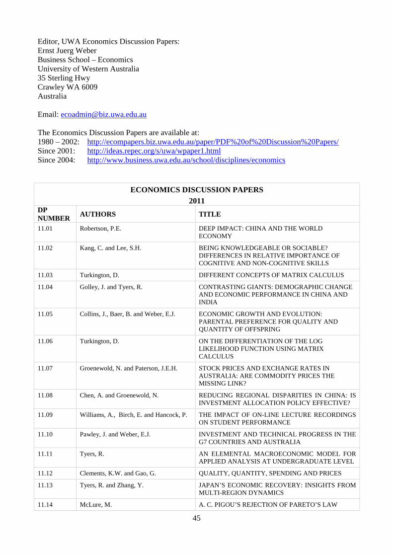
Editor, UWA Economics Discussion Papers: Ernst Juerg Weber Business School – Economics University of Western Australia 35 Sterling Hwy Crawley WA 6009 Australia Email: ecoadmin@biz.uwa.edu.au The Economics Discussion Papers are available at: 1980 – 2002: http://ecompapers.biz.uwa.edu.au/paper/PDF%20of%20Discussion%20Papers/ Since 2001: http://ideas.repec.org/s/uwa/wpaper1.html Since 2004: http://www.business.uwa.edu.au/school/disciplines/economics

ECONOMICS DISCUSSION PAPERS 2011

DP NUMBER AUTHORS TITLE

11.01 Robertson, P.E. DEEP IMPACT: CHINA AND THE WORLD ECONOMY

11.02 Kang, C. and Lee, S.H. BEING KNOWLEDGEABLE OR SOCIABLE? DIFFERENCES IN RELATIVE IMPORTANCE OF COGNITIVE AND NON-COGNITIVE SKILLS

11.03 Turkington, D. DIFFERENT CONCEPTS OF MATRIX CALCULUS

11.04 Golley, J. and Tyers, R. CONTRASTING GIANTS: DEMOGRAPHIC CHANGE AND ECONOMIC PERFORMANCE IN CHINA AND INDIA

11.05 Collins, J., Baer, B. and Weber, E.J. ECONOMIC GROWTH AND EVOLUTION: PARENTAL PREFERENCE FOR QUALITY AND QUANTITY OF OFFSPRING

11.06 Turkington, D. ON THE DIFFERENTIATION OF THE LOG LIKELIHOOD FUNCTION USING MATRIX CALCULUS

11.07 Groenewold, N. and Paterson, J.E.H. STOCK PRICES AND EXCHANGE RATES IN AUSTRALIA: ARE COMMODITY PRICES THE MISSING LINK?

11.08 Chen, A. and Groenewold, N. REDUCING REGIONAL DISPARITIES IN CHINA: IS INVESTMENT ALLOCATION POLICY EFFECTIVE?

11.09 Williams, A., Birch, E. and Hancock, P. THE IMPACT OF ON-LINE LECTURE RECORDINGS ON STUDENT PERFORMANCE

11.10 Pawley, J. and Weber, E.J. INVESTMENT AND TECHNICAL PROGRESS IN THE G7 COUNTRIES AND AUSTRALIA

11.11 Tyers, R. AN ELEMENTAL MACROECONOMIC MODEL FOR APPLIED ANALYSIS AT UNDERGRADUATE LEVEL

11.12 Clements, K.W. and Gao, G. QUALITY, QUANTITY, SPENDING AND PRICES

11.13 Tyers, R. and Zhang, Y. JAPAN’S ECONOMIC RECOVERY: INSIGHTS FROM MULTI-REGION DYNAMICS

11.14 McLure, M. A. C. PIGOU’S REJECTION OF PARETO’S LAW

45

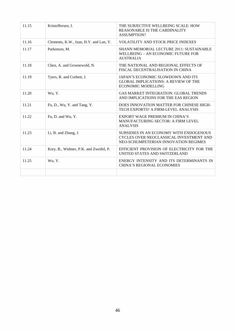
11.15 Kristoffersen, I. THE SUBJECTIVE WELLBEING SCALE: HOW REASONABLE IS THE CARDINALITY ASSUMPTION?

11.16 Clements, K.W., Izan, H.Y. and Lan, Y. VOLATILITY AND STOCK PRICE INDEXES

11.17 Parkinson, M. SHANN MEMORIAL LECTURE 2011: SUSTAINABLE WELLBEING – AN ECONOMIC FUTURE FOR AUSTRALIA

11.18 Chen, A. and Groenewold, N. THE NATIONAL AND REGIONAL EFFECTS OF FISCAL DECENTRALISATION IN CHINA

11.19 Tyers, R. and Corbett, J. JAPAN’S ECONOMIC SLOWDOWN AND ITS GLOBAL IMPLICATIONS: A REVIEW OF THE ECONOMIC MODELLING

11.20 Wu, Y. GAS MARKET INTEGRATION: GLOBAL TRENDS AND IMPLICATIONS FOR THE EAS REGION

11.21 Fu, D., Wu, Y. and Tang, Y. DOES INNOVATION MATTER FOR CHINESE HIGH-TECH EXPORTS? A FIRM-LEVEL ANALYSIS

11.22 Fu, D. and Wu, Y. EXPORT WAGE PREMIUM IN CHINA’S MANUFACTURING SECTOR: A FIRM LEVEL ANALYSIS

11.23 Li, B. and Zhang, J. SUBSIDIES IN AN ECONOMY WITH ENDOGENOUS CYCLES OVER NEOCLASSICAL INVESTMENT AND NEO-SCHUMPETERIAN INNOVATION REGIMES

11.24 Krey, B., Widmer, P.K. and Zweifel, P. EFFICIENT PROVISION OF ELECTRICITY FOR THE UNITED STATES AND SWITZERLAND

11.25 Wu, Y. ENERGY INTENSITY AND ITS DETERMINANTS IN CHINA’S REGIONAL ECONOMIES

46

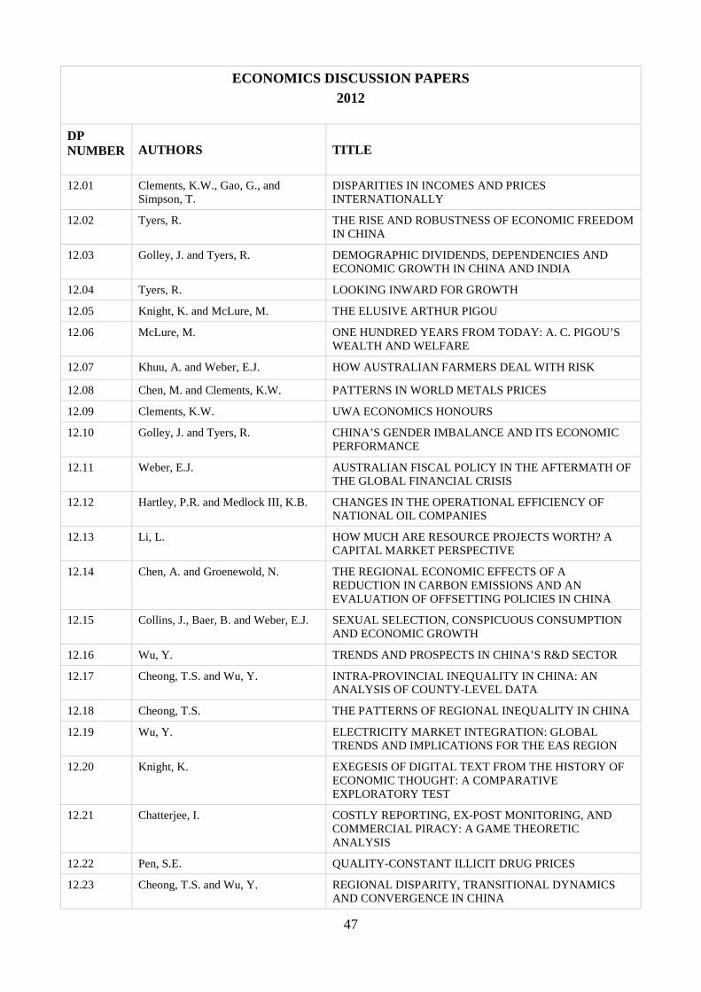
ECONOMICS DISCUSSION PAPERS 2012

DP NUMBER AUTHORS TITLE

12.01 Clements, K.W., Gao, G., and Simpson, T.

DISPARITIES IN INCOMES AND PRICES INTERNATIONALLY

12.02 Tyers, R. THE RISE AND ROBUSTNESS OF ECONOMIC FREEDOM IN CHINA

12.03 Golley, J. and Tyers, R. DEMOGRAPHIC DIVIDENDS, DEPENDENCIES AND ECONOMIC GROWTH IN CHINA AND INDIA

12.04 Tyers, R. LOOKING INWARD FOR GROWTH

12.05 Knight, K. and McLure, M. THE ELUSIVE ARTHUR PIGOU

12.06 McLure, M. ONE HUNDRED YEARS FROM TODAY: A. C. PIGOU’S WEALTH AND WELFARE

12.07 Khuu, A. and Weber, E.J. HOW AUSTRALIAN FARMERS DEAL WITH RISK

12.08 Chen, M. and Clements, K.W. PATTERNS IN WORLD METALS PRICES

12.09 Clements, K.W. UWA ECONOMICS HONOURS

12.10 Golley, J. and Tyers, R. CHINA’S GENDER IMBALANCE AND ITS ECONOMIC PERFORMANCE

12.11 Weber, E.J. AUSTRALIAN FISCAL POLICY IN THE AFTERMATH OF THE GLOBAL FINANCIAL CRISIS

12.12 Hartley, P.R. and Medlock III, K.B. CHANGES IN THE OPERATIONAL EFFICIENCY OF NATIONAL OIL COMPANIES

12.13 Li, L. HOW MUCH ARE RESOURCE PROJECTS WORTH? A CAPITAL MARKET PERSPECTIVE

12.14 Chen, A. and Groenewold, N. THE REGIONAL ECONOMIC EFFECTS OF A REDUCTION IN CARBON EMISSIONS AND AN EVALUATION OF OFFSETTING POLICIES IN CHINA

12.15 Collins, J., Baer, B. and Weber, E.J. SEXUAL SELECTION, CONSPICUOUS CONSUMPTION AND ECONOMIC GROWTH

12.16 Wu, Y. TRENDS AND PROSPECTS IN CHINA’S R&D SECTOR

12.17 Cheong, T.S. and Wu, Y. INTRA-PROVINCIAL INEQUALITY IN CHINA: AN ANALYSIS OF COUNTY-LEVEL DATA

12.18 Cheong, T.S. THE PATTERNS OF REGIONAL INEQUALITY IN CHINA

12.19 Wu, Y. ELECTRICITY MARKET INTEGRATION: GLOBAL TRENDS AND IMPLICATIONS FOR THE EAS REGION

12.20 Knight, K. EXEGESIS OF DIGITAL TEXT FROM THE HISTORY OF ECONOMIC THOUGHT: A COMPARATIVE EXPLORATORY TEST

12.21 Chatterjee, I. COSTLY REPORTING, EX-POST MONITORING, AND COMMERCIAL PIRACY: A GAME THEORETIC ANALYSIS

12.22 Pen, S.E. QUALITY-CONSTANT ILLICIT DRUG PRICES

12.23 Cheong, T.S. and Wu, Y. REGIONAL DISPARITY, TRANSITIONAL DYNAMICS AND CONVERGENCE IN CHINA

47

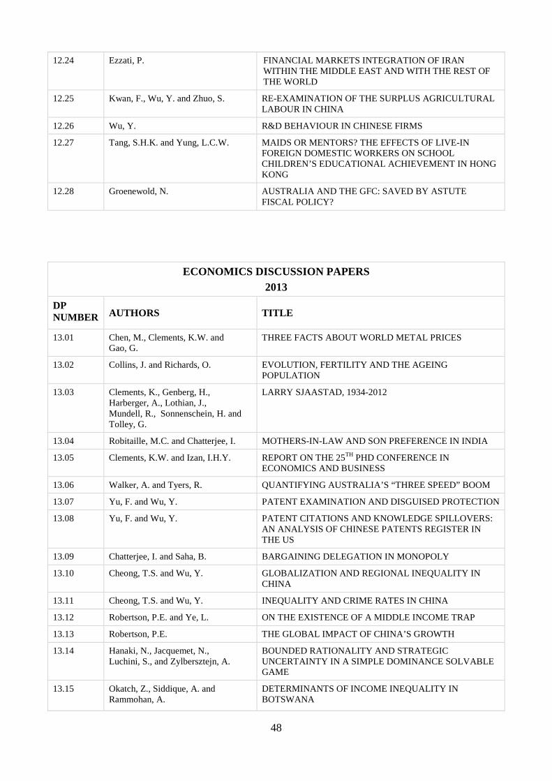
12.24 Ezzati, P. FINANCIAL MARKETS INTEGRATION OF IRAN WITHIN THE MIDDLE EAST AND WITH THE REST OF THE WORLD

12.25 Kwan, F., Wu, Y. and Zhuo, S. RE-EXAMINATION OF THE SURPLUS AGRICULTURAL LABOUR IN CHINA

12.26 Wu, Y. R&D BEHAVIOUR IN CHINESE FIRMS

12.27 Tang, S.H.K. and Yung, L.C.W. MAIDS OR MENTORS? THE EFFECTS OF LIVE-IN FOREIGN DOMESTIC WORKERS ON SCHOOL CHILDREN’S EDUCATIONAL ACHIEVEMENT IN HONG KONG

12.28 Groenewold, N. AUSTRALIA AND THE GFC: SAVED BY ASTUTE FISCAL POLICY?

ECONOMICS DISCUSSION PAPERS 2013

DP NUMBER AUTHORS TITLE

13.01 Chen, M., Clements, K.W. and Gao, G.

THREE FACTS ABOUT WORLD METAL PRICES

13.02 Collins, J. and Richards, O. EVOLUTION, FERTILITY AND THE AGEING POPULATION

13.03 Clements, K., Genberg, H., Harberger, A., Lothian, J., Mundell, R., Sonnenschein, H. and Tolley, G.

LARRY SJAASTAD, 1934-2012

13.04 Robitaille, M.C. and Chatterjee, I. MOTHERS-IN-LAW AND SON PREFERENCE IN INDIA

13.05 Clements, K.W. and Izan, I.H.Y. REPORT ON THE 25TH PHD CONFERENCE IN ECONOMICS AND BUSINESS

13.06 Walker, A. and Tyers, R. QUANTIFYING AUSTRALIA’S “THREE SPEED” BOOM

13.07 Yu, F. and Wu, Y. PATENT EXAMINATION AND DISGUISED PROTECTION

13.08 Yu, F. and Wu, Y. PATENT CITATIONS AND KNOWLEDGE SPILLOVERS: AN ANALYSIS OF CHINESE PATENTS REGISTER IN THE US

13.09 Chatterjee, I. and Saha, B. BARGAINING DELEGATION IN MONOPOLY

13.10 Cheong, T.S. and Wu, Y. GLOBALIZATION AND REGIONAL INEQUALITY IN CHINA

13.11 Cheong, T.S. and Wu, Y. INEQUALITY AND CRIME RATES IN CHINA

13.12 Robertson, P.E. and Ye, L. ON THE EXISTENCE OF A MIDDLE INCOME TRAP

13.13 Robertson, P.E. THE GLOBAL IMPACT OF CHINA’S GROWTH

13.14 Hanaki, N., Jacquemet, N., Luchini, S., and Zylbersztejn, A.

BOUNDED RATIONALITY AND STRATEGIC UNCERTAINTY IN A SIMPLE DOMINANCE SOLVABLE GAME

13.15 Okatch, Z., Siddique, A. and Rammohan, A.

DETERMINANTS OF INCOME INEQUALITY IN BOTSWANA

48

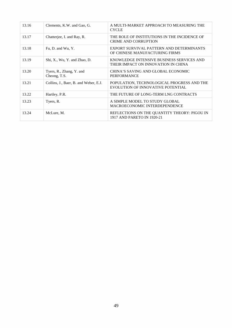
13.16 Clements, K.W. and Gao, G. A MULTI-MARKET APPROACH TO MEASURING THE CYCLE

13.17 Chatterjee, I. and Ray, R. THE ROLE OF INSTITUTIONS IN THE INCIDENCE OF CRIME AND CORRUPTION

13.18 Fu, D. and Wu, Y. EXPORT SURVIVAL PATTERN AND DETERMINANTS OF CHINESE MANUFACTURING FIRMS

13.19 Shi, X., Wu, Y. and Zhao, D. KNOWLEDGE INTENSIVE BUSINESS SERVICES AND THEIR IMPACT ON INNOVATION IN CHINA

13.20 Tyers, R., Zhang, Y. and Cheong, T.S.

CHINA’S SAVING AND GLOBAL ECONOMIC PERFORMANCE

13.21 Collins, J., Baer, B. and Weber, E.J. POPULATION, TECHNOLOGICAL PROGRESS AND THE EVOLUTION OF INNOVATIVE POTENTIAL

13.22 Hartley, P.R. THE FUTURE OF LONG-TERM LNG CONTRACTS

13.23 Tyers, R. A SIMPLE MODEL TO STUDY GLOBAL MACROECONOMIC INTERDEPENDENCE

13.24 McLure, M. REFLECTIONS ON THE QUANTITY THEORY: PIGOU IN 1917 AND PARETO IN 1920-21

49