inflation and unemployment as determinants of · pdf file155 inflation and unemployment as...

This PDF is a selection from an out-of-print volume from the National Bureauof Economic Research

Volume Title: Reform, Recovery, and Growth: Latin America and the MiddleEast

Volume Author/Editor: Rudiger Dornbusch and Sebastian Edwards, eds.

Volume Publisher: University of Chicago Press

Volume ISBN: 0-226-15745-4

Volume URL: http://www.nber.org/books/dorn95-1

Conference Date: December 17-18, 1992

Publication Date: January 1995

Chapter Title: Inflation and Unemployment as Determinants of Inequalityin Brazil: The 1980s

Chapter Author: Eliana Cardoso, Andre Urani, Andre Urani

Chapter URL: http://www.nber.org/chapters/c7655

Chapter pages in book: (p. 151 - 176)

5 Inflation and Unemployment as Determinants of Inequality in Brazil: The 1980s Eliana Cardoso, Ricardo Paes de Barros, and Andre Urani

5.1 Introduction

Inequality in Brazil has shown extreme oscillations in short periods of time. The benefits from growth in the 1960s went disproportionately to the rich, and the costs of the 1980s stagnation fell disproportionately on the poor. The income of the richest 10% of the active population divided by the income of the poorest 10% of the population increased from a factor of 22 in 1960, to 40 in 1970,41 in 1980, and 80 in 1989. It declined in 1991 . I

This paper studies the oscillations of income distribution in Brazil during the 1980s. Using monthly data for the six largest metropolitan areas, it claims that inequality responded to megainflation and the sharp oscillations in employment. As opposed to what happened in the 1960s, education cannot explain the change in inequality in the 1980s.

Economists agree that behind the vast inequality of income distribution in Brazil lies an extremely unequal education distribution. Barros et al. (1992)

Eliana Cardoso is the William Clayton Professor of Economics at the Fletcher School of Law and Diplomacy at Tufts University and a research associate of the National Bureau of Economic Research. Ricardo Paes de Barros is assistant professor of economics at Yale University and a research associate of the Instituto de Pesquisa Economica Aplicada in Rio de Janeiro. Andre Urani is adjunct professor of economics at the Universidade Federal do Rio de Janeiro and a research associate of the Instituto de Pesquisa Economica Aplicada in Rio de Janeiro.

The authors thank Renata Patricia Jeronimo, Danielle Carusi Machado, and Carlos Henrique Leite Corseuil for excellent research assistance.

1. These numbers are calculated from the annual household surveys called Pesquisa Nacional de Domicilios and do not cover the same universe as the monthly employment surveys called Pesquisa Mensal de Emprego (PMEs), which are used in this paper. The PMEs show that the income of the richest 10% of the active population in the metropolitan areas divided by the income of the poorest 10% of the population, after peaking in mid-1990, was declining during 1991. It averaged a factor of 72 during the last quarter of 1991.

151

152 Eliana Cardoso, Ricardo Paes de Barros, and Andre Urani

show that, if all wage differentials by education level were eliminated, the inequality in labor income in Brazil would be reduced by almost 50%.’

But even if we believe that education plays a major role in explaining inequality, we do not want to attribute the big deterioration of distribution that occurred from 1987 to 1989 to changes in the distribution of education. The poor do not lose their skills so fast, nor do the rich acquire in such a short period of time the education that transforms them into productivity prodigies. On the other hand, recessions and megainflations do play a role in explaining exacerbated income inequality.

Over the past decade, inequality in Brazil has shown only a minor change in trend but extreme short-run variations (fig. 5.1). The contribution of this paper is to decompose inequality into two components: inequality within and between groups with the same number of years of schooling. Our objective is to identify macroeconomics as an important explanation for the short-run variations. Specifically, we offer two conclusions: inflation promotes increased inequality and unemployment increases inequality.

These conclusions do not surprise, but they have not been formally docu- mented before nor has their extreme effect, as shown in figure 5.1, been noted. Needless to say, on the evidence shown here, anyone concerned with inequality would focus on macroeconomic stability as a central policy for increased equality.

A recession worsens income distribution because of its effect on employment. In a recession, unskilled workers are the first to lose their jobs, as firms hoard the trained labor force. In the recovery, unskilled workers get back their jobs, and inequality diminishes. One must also take into account the fact that a recession has lasting effects on income distribution. During the recession the middle-class groups sell their assets to smooth consumption, assets that they might not be able to earn back during a recovery.

Figure 5.2 shows the recession of 1983-84 and the decline in real income during 1989-91. Add to the recession all the failed stabilization programs and observe that the poor have little room to cope with the radical policy moves that produce sectoral dislocation of resources and employment.

Figure 5.3 shows inflation during the 1980s. Inflation can increase inequality in three ways. First, if high wages benefit from more perfect indexation, inequality increases. The empirical evidence shows that perfect indexation does not exist and that all labor groups suffer real losses during episodes of high inflation. This paper also shows that in Brazil the group with five to eight years of education lost more than other groups in the 1980s.

Second, the inflation tax reduces disposable income. Although the inflation tax does not affect those individuals below the poverty line due to their negligi- ble average cash holdings, it may wipe out the savings of the middle class

2. See Paes de Barros and Reis (1989); Sedlacek and Paes de Barros (1989); Lauro Rarnos (1991).

153 Inflation and Unemployment as Determinants of Inequality in Brazil

0.4 1 I

D 25

0 2 -

0 . 1 5 J R D a1 a2 a3 a4 a5 a6 a7 aa a9 90 9 1

- Total-0.40 - - - Within-.25 - Between

Fig. 5.1 Temporal evolution of inequality in Brazil, 198291 Note: Twelve-month moving averages for six metropolitan areas of the Theil indices for total, within, and between educational groups inequality.

I I

50-

4 o a 8 2 8 3 84 85 86 87 88 89 90 91

Y W

110- 1

100-

80-

70-

80-

50-

4 o a 8 2 8 3 84 85 86 87 88 89 90 91

Y W

Fig. 5.2 Real income, Brazil, 198291 Note: Average for six metropolitan areas.

and increase the number of poor. In this sense it increases poverty and widens inequality of income (see Cardoso 1992).

Third, inflation will redistribute assets in favor of the group better able to play the financial markets. Inflation is difficult to predict, and nominal interest rates may fail to reflect changing inflation rates. As a result there will be trans-


80

Fig. 5.3 Note: Three-month moving average; percentage per month.

Inflation rate, Brazil, 1985-92

fers of wealth between creditors and debtors. This will be true of all debtors and creditors linked by indebtedness in the form of bonds, mortgages, and sales contracts, and will also be reflected in the stock market. When inflation reaches 1,000%, big gains and losses can be made overnight. The middle- income groups will certainly lose compared to the groups who have better information, access to expensive technical advice, and flexibility.

The costs of inflation for wage earners also include oscillations in their real income. For individuals who are liquidity constrained, the significant oscillation in their real wages means that they cannot smooth consumption or that their real disposable income will be eroded if they try to carry cash from one month to the next.

This paper explores the impact of unemployment and inflation on Brazilian inequality in the 1980s. The data we use is from Pesquisa Mensal de Emprego (PME), a monthly employment survey conducted by the Instituto Brasileiro de Geografia e Estatistica.3 These surveys do not cover money holdings and capi- tal gains. Our measures of inequality capture only inequality in labor earnings, and thus the impact of inflation that we can estimate derives from imperfect indexation. Further information is needed to identify the impact on inequality from the inflation tax and the redistribution of assets.

The paper is organized as follows. Section 5.2 sets the background with a

3. The universe of analysis and the data are described in the appendix


summary of what is known about income distribution in Brazil. It also de- scribes the inequality measures used in the paper. Section 5.3 contains the empirical evidence, which is based on monthly survey data for the six largest metropolitan areas of Brazil between 1982 and 1991. The empirical analysis considers the relationship between inequality in labor income and three variables: the inflation rate, the unemployment rate, and the income differentials by educational level. The methodology and the evidence are summarized in section 5.4, which gives our conclusions.

5.2 Brazilian Income Distribution

5.2.1 Background

In no country has the academic debate on growth versus equality been sharper than in Brazil. In the 1970s the core of the discussion was whether the poor benefited from growth during the 1965-74 “miracle” and whether they might have done better under different policies4 Today the discussion must evaluate the costs of bad macroeconomics in the 1980s.

The complexity of statistical problems surrounding income distribution data in Brazil is serious enough to provoke skepticism. However, a few stylized facts are widely accepted.

Unequal income distribution. Brazil (with a Gini coefficient equal to 0.6 in 1990) has one of the most unequal income distributions in the world. Social indicators look worse than in any other country with the same income per capita. Table 5.1 compares economic and social indicators in Brazil with those of Latin American countries with a population of more than 10 million people. Brazil does poorly. Although in 1990 it had the highest dollar income per capita in the region, infant mortality was three times that of Chile, the illiteracy ratio was four times that of Argentina, and Brazilians could expect to live four years less than me xi can^.^

Regional inequality. National averages of economic and social indicators hide extreme disparities. Regional inequality is severe.6 For instance, the interstate range of income in Brazil is seven to one.’ Table 5.2 shows the range of economic and social indicators for the poorest and richest regions and states. Ca- valcanti de Albuquerque (1991) compares the index of human development for

4. See for instance Camargo and Giambiagi (1991); Fields (1977); Fishlow (1980); Morley

5. For measures of poverty see Hoffmann (1989) and Ravallion and Datt (1991). 6. See for instance Vinod (1987); Maddison and associates (1989). 7. Interstate disparity is two to one in the United States, where Mississippi’s per capita income

was half that of Connecticut’s in 1991 (US. Department of Commerce, Survey of Currenr Busi- ness, vol. 72 [4] [April 19921 table A).

(1982); Pfeffermann and Webb (1979); Taylor et al. (1980).


Table 5.1 Economic and Social Indicators in Latin American Countries with More than 10 Million People

~ ~ ~~ -

GDP per Life Adult Mean Population Head Gini Population Expectancy Illiteracy Years Infant (million$) ($) (Index) Growth (years) Rate in Mortality

Country (1990) (1990) (1989) (70)" (1990) (%)b Schoolc Rated

Brazil Mexico Argentina Colombia Peru Venezuela Chile Ecuador

150.4 86.2 32.3 32.3 21.7 19.7 13.2 10.3

2,680 2,490 2,370 1,260 1,160 2,560 1,940

980

0.625 2.2 2.0

0.461 1.3 0.515 2.0

2.3 0.498 2.7

I .7 2.4

66 19 3.9 60 70 13 4.7 40 71 5 8.7 31 69 13 5.7 39 63 15 6.4 82 70 12 6.3 35 72 7 7.5 20 66

Sources: World Bank (1992); Fiszbein and Psacharopoulos (1992); Barros et al. (1992) aPercentage per year between 1980 and 1989. bPercentage of the total population that is fifteen years old or older. 'For individuals twenty-five years old or older. "For one thousand live births.

Table 5.2 Economic and Social Indicators in Brazil: Poorest and Richest Regions and States, 1988

Poorest states Piaui Paraiba

Richest states S2o Paulo Distrito Federal

Poorest region: Northeast Richest region: Southeast Brazil

GDP per Head Life Expectancy Literacy Ratio ($ of 1988) (years) (%)

594 62.6 718 51.9

55.9 63.1

3,503 67.0 90.5 4,215 68.9 89.5 1,005 58.8 63.5 2,989 67.1 88.2 2.24 1 64.9 81.1

Source: Cavalcanti de Albuquerque (1991).

Brazilian states with indices of other nations. Rio Grande do Sul is as advanced as Portugal, South Korea, or Argentina, while Paraiba performs as badly as Kenya and worse than Bolivia.

Destitution remains predominantly a rural phenomenon even if the gap between the urban and the rural living standards has declined in the last twenty years (table 5.3). In 1988 rural income was still 60% of urban income.

Inequality has roots in history. In the colonial economy, rents from abundant natural resources were monopolized by the state and by large landlords from


Table 5.3 Indices of Urban-Rural Disparity, Brazil, 1970-88

Income Index Human Development Indexa (urban income = 100) (urban index = 100)

Rural Northeast Rural South Rural Brazil Rural Northeast Rural South Rural Brazil

1970 30 53 37 39 71 52 1980 47 70 53 55 83 64 1988 52 78 60 64 84 69

Source: Cavalcanti de Albuquerque (1991)

Portugal. The labor force was slaves. After the abolition of slavery, there was no land reform. Official policy kept labor cheap and uneducated.

Poorly managed social programs. Brazil spends as much as Korea on social programs, but it spends poorly. The Brazilian share of social service expenditure by government in GDP is as high as or even higher than that of other middle-income developing countries, but Brazilian social welfare indicators are strikingly low.

The reasons for such an unsatisfactory social performance are twofold: public resources are poorly managed and are not efficiently targeted. The poorest 19% of the population (with less than one-quarter of a minimum wage per household member) receives 6% of social benefits. An estimated 78% of all spending on health is devoted to high-cost curative hospital services and only 22% to basic preventive health care, such as immunization programs, malaria control, and maternal and child health. In education, the government supports free tuition in universities although the cost of educating each university student is eighteen times higher than government expenditure per student at the primary and secondary level combined.*

Increasing inequality. From 1960 to 1975 the degree of inequality increased continuously. While Fishlow (1972) emphasized the role of government policy in squeezing real wages, Langoni (1 973) stressed nonpolicy forces inherent in a situation of fast growth with a shortage of educated labor. Despite the political debate that surrounded the two studies, there is no necessary conflict between the two views. The gap between rich and poor increased not only as a result of the increase of the real wage of skilled labor but also because the real wage of unskilled labor fell, in part as a result of the rise in inflation before 1964 and from the mid-1960s recession, which validated the incomes policy of imperfect indexation. Along with this explanation, education plays a central

8. The World Bank (1988) and Barros et al. (1992) offer analyses and critiques of social spending in Brazil.


role in explaining the worsening in the distribution of income in Brazil between 1960 and 1975.

The education system has a double relationship with the degree of inequality in income. Since the level of education is so low, educational expansion tends to increase the inequality in education and consequently the inequality in income. This is the composition or Kuznets effect. On the other hand, education expansion was considered to be too slow in comparison to the rate of economic growth and technological change. As a consequence, a relative shortage of educated and skilled workers led to a widening of the wage differential between workers with different years of schooling.

Barros et al. (1992) shows that two-thirds of the increase in inequality between 1960 and 1970 can be attributed to education. But the same paper also shows that education has a minor role in explaining what happened in the late 1970s and in the first half of the 1980s. In this paper we will show that unemployment and inflation generated the extreme oscillations in inequality ob- served in the 1980s.

5.2.2 Measuring Inequality

Changes in income inequality are usually described by changes in a scalar measure of inequality such as the Gini or the Theil index. A scalar measure completely ranks a set of income distributions in terms of increasing inequality, but alternative scalar measures do not necessarily rank a set of distributions in the same way. We lessen this problem by using six different measures.

The Lorenz curve, L(p) , shows the share of the total income that is appro- priated by the poorest p% of the population and is defined as

for 0 5 p 5 I . F is the cumulative distribution of the random variable Z, which represents labor earnings, and c~ is the mean of Z. Figure 5.4 illustrates the behavior of the Lorenz curves. The continuous line represents income distribution in the early 1980s. In 1990 the Lorenz curve shifts out as inequality increases, and in 1991 it shifts in as inequality decreases.

Based on the Lorenz curve, we can estimate a second measure of inequality: the relation between the income share of the richest 10% of the population and the income share of the poorest 40%. We call this measure the spread, S.

(2) S [I - L(0.9)]/L(0.4)

We also use the Gini coefficient as a measure of inequality. The Gini coefficient is defined as

(3) G (1 - 2L(p)) dp. I"'

159 Inflation and Unemployment a s Determinants of Inequality in Brazil

JUL W J U N 83

JAN W J U N 90 . ... ... .

Fig. 5.4 Lorenz curves, Brazil, 1980-91

The next inequality measure is the Theil index, 7: defined as

(4) T = E [ ( Z / p ) ln(Z/p)],

where E is the expectation operator, and Z has already been defined as a random variable representing labor earning^.^

Inspection of monthly estimates for the spread, the Gini coefficient, and the Theil index, from January 1980 to December 1991, indicates the presence of outliers. We consider as outliers any estimate that diverges from the mean by more than two standard deviations. Since outliers can strongly influence our empirical analysis, we discarded them. The identification of outliers was done for each metropolitan area separately. Having identified an outlier, all inequality measures for that point in time and metropolitan area were discarded.

Next we decompose inequality.'O The objective of the decomposition is to isolate the contribution of changes associated with education from all other sources of change in inequality. We divide the population in each metropolitan region into five subgroups. In each of these subgroups, all workers have the same level of education according to the number of completed years of schooling: less than one, one to four (elementary school), five to eight, nine to eleven, and twelve or more years. Based on this division we compute a measure of the average income inequality within groups, I, defined as

( 5 )

9. Monthly estimates for the spread, the Gini coefficient, and the Theil index for the six largest metropolitan areas of Brazil are available upon request.

10. The variables used in the decomposition analysis spread over the period May 1982 and December 199 1, because the surveys do not cover information on the level of education of workers before May 1982.


where is the inequality within subgroup i as measured by the Theil index; {a ,} is a system of weights, a, 2 0 and xa, = 1.

The measure of inequality within groups, I, can change either because the inequality within groups, {Wz] has changed or because the weights, {a , ] , have changed. Because we do not want our measure I to be affected by changes in the distribution of the population by educational level, we define the weight of each subgroup i as the average of the 1980-91 shares in total population in each metropolitan area. Therefore, the weights are constant, and only variations in { m) can affect the measure of inequality within groups, I .

The measure of the inequality between groups, B, is defined as

(6) B E T - I .

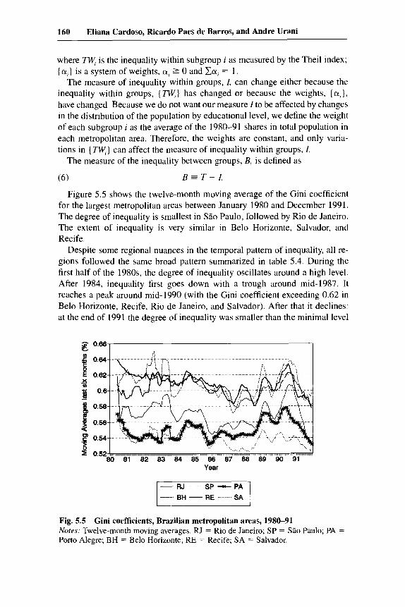
Figure 5.5 shows the twelve-month moving average of the Gini coefficient for the largest metropolitan areas between January 1980 and December 199 1. The degree of inequality is smallest in Siio Paulo, followed by Rio de Janeiro. The extent of inequality is very similar in Belo Horizonte, Salvador, and Recife.

Despite some regional nuances in the temporal pattern of inequality, all regions followed the same broad pattern summarized in table 5.4. During the first half of the 1980s, the degree of inequality oscillates around a high level. After 1984, inequality first goes down with a trough around mid-1987. It reaches a peak around mid- 1990 (with the Gini coefficient exceeding 0.62 in Belo Horizonte, Recife, Rio de Janeiro, and Salvador). After that it declines: at the end of 199 1 the degree of inequality was smaller than the minimal level

0.68 , I

0.64

0.62

0.6

0.58

0.58

0.54

05280 81 82 83 84 85 86 87 88 89 90 91 Year

BH -RE SA

Gini coefficients, Brazilian metropolitan areas, 1980-91 Notes: Twelve-month moving averages. RJ = Rio de Janeiro; SP = S l o Paulo; PA = Porto Alegre; BH = Belo Horizonte; RE = Recife; SA = Salvador.


Table 5.4 Inequality Indices: Twelve-Month Average for Six Metropolitan Areas, 1981-91

Theil Gini

1981 1982 1983 1984 1985 1986 1987 1988 1989 1990 1991

0.68 0.73 0.69 0.69 0.64 0.65 0.63 0.67 0.69 0.73 0.65

0.58 0.59 0.58 0.59 0.58 0.57 0.57 0.57 0.58 0.60 0.56

reached during the 1980s (the average for the six metropolitan areas was 0.56 in 1991).

The temporal pattern for the other inequality indicators (the Theil index and the spread) follow a very similar pattern. The appendix table 5A.1 shows the high degree of correlation between the different inequality indicators for each metropolitan region.

5.3 The Empirical Evidence

5.3.1 Sources of Inequality

We believe that education has an important role in determining inequality but that it cannot explain the cyclical pattern followed by inequality in the 1980s. To determine whether education contributed to the cyclical pattern of the degree of income inequality in the 1980s, we compare the temporal evolution of the Theil index, with the temporal evolution for the average inequality within groups, I. By construction, I is not affected by changes either in the educational composition of the labor force or in the wage differentials by education level. Hence, if I and T follow the same pattern, we can say that the events affecting the evolution of the inequality in the 1980s are unrelated to changes associated with education.

We begin by investigating the temporal evolution of the average inequality within groups, I, and the inequality between groups, B. We can do this only after March 1982, when questions on education were introduced in the PME questionnaire. Both I and B behave similarly across regions, and we can thus concentrate our discussion on the average across regions."

11, Monthly estimates of the two components of the Theil measure for each of the six metropolitan areas are available upon request.


Figure 5.1 shows the temporal evolution of {he average across metropolitan areas of the Theil index, of the index of inequality within groups, Z, and of the index of inequality between groups, B. Both the Theil index and the index for inequality within groups display the same cyclical pattern. In addition, the index for inequality within groups shows a decreasing trend. On the other hand, the index of inequality between groups, B, displays almost no cyclical pattern and a clear increasing trend.

In summary, the temporal pattern of the overall inequality can be decom- posed into three components: (1) a complete cycle from mid-1984 to the end of 1991 that is perfectly matched by the temporal evolution of the inequality within group; (2) a decreasing trend in inequality caused by a decline in the Theil within groups; and (3) an upward trend in inequality caused by an increase in the inequality between groups. As a result, from mid-1982 to the end of 1991, the overall inequality went through a complete cycle with a slightly decreasing trend.

A consequence of the opposite trends in inequality within groups and inequality between groups is an increase in the power of explanation of education to account for the level of inequality at a point in time. We can measure the “explanatory power of education” by the ratio between the indices of inequality between and within groups, BII. This ratio increases over the period. Therefore, over the 1980s, even though education does not explain the variations in inequality during the period, the static relationship between education and the level of the overall inequality in 1991 is even stronger than in 1982.

We also use an alternative procedure to investigate the relative contribution of education to the cyclical fluctuations in inequality. We first identify four periods, which are characterized by relatively big or small inequality: July 1982 to June 1983 (big); July 1986 to June 1987 (small); January 1990 to June 1990 (big); July 1991 to December 1991 (small). Then we decompose the change in overall inequality between each of these periods in two components: a change in inequality within groups and a change in inequality between groups. Table 5.5 shows that the decline in inequality between 1982-83 and 1986-87 is almost entirely explained by a decline in inequality within groups. The increase in inequality between 1986-87 and 1990 is explained by an increase in inequality in both indices of inequality. Finally, the decline in inequality between 1990 and 1991 is fully explained by the variation in inequality within groups.

Estimates by metropolitan area (in the appendix tables) corroborate that for

Table 5.5 Decomposing the Variation in Inequality (average of all metropolitan areas)

~

To AT AIIAT ABIAT

July 82-June 83 July 86-June 87 -0.053 0.94 0.06 July 86-June 87 Jan. 90-June 90 0.102 0.50 0.50 Jan. 90-June 90 July 9 1-Dec. 9 1 -0.095 1.02 -0.02


10-

8-

8-

7-

6-

5-

4-

3-

f E

A . . . . . . . . . . . . . . . . . . . . . . . . . . . . . . . . . . . ,-., ( . ............. j+.+& ....................... ..A.f.. ............................................. ..{

*: I ,

............................................................................... I

2' 80 81 82 83 84 85 88 87 88 89 90 91

Year

-1 Fig. 5.6 Unemployment rate in largest metropolitan areas, Brazil, 1980-91 Nofes: Twelve-month moving averages. For definitions of abbreviations, see note to fig. 5.5.

all areas the within component contributes more than the index for inequality between groups to the decline in inequality from 1982-83 to 1986-87 and from 1990 to 1991. The results are mixed for the period in which inequality increases. In Belo Horizonte and Recife the between component accounts for the major part of the increase in inequality; in Salvador both components account equally for the change in inequality; in Rio de Janeiro the within component accounts for the major part of the change in the overall level of inequality.

Having argued that the cyclical pattern followed by the level of the income inequality in Brazil is unrelated to changes associated with education, we turn to the analysis of unemployment and inflation.

5.3.2 Unemployment and Inflation as Determinants of Inequality

We first describe the evolution of inflation and unemployment in the 1980s. The inflation rates calculated from regional price indices are practically the

same in all metropolitan areas. Between 1981 to mid-1983, the inflation rate was relatively stable at approximately 6% per month (fig. 5.3). From mid-1983 to the beginning of 1986, inflation doubled, it disappeared in March 1986 with the Cruzado Plan and returned at full speed in 1987, when it accelerated fast, reaching 40% per month in 1989. Inflation declined in 1990 to 15% per month.

The evolution of the unemployment rate between 1980 and 1991 by metropolitan area is shown in figure 5.6.'* Recife has the highest unemployment rates and Rio de Janeiro the lowest. In all metropolitan areas the unemploy-

12. An individual is defined as unemployed if he or she is ten or more years old and was not employed at the time of the interview but was actively looking for a job in the week prior to the interview.


ment rates declined over the period. The decline was larger in Belo Horizonte and smaller in Silo Paulo. Overall the oscillation of unemployment during the period follows a similar pattern in all metropolitan areas.

From 1980 to 1985 the unemployment rate went through two small cycles. It peaked at approximately 9% in the third quarter of 1981, declined to 6% in the third quarter of 1982, and increased to almost 8% in mid-1984. From mid- 1984 to the end of 1986, there was a sharp decline in unemployment to less than 4%. Finally, from 1987 to 1991, the unemployment rate showed a slight increasing trend.

The short-run fluctuations in unemployment in the first half of the 1980s and the sharp decline from 1985 to 1987 quite closely match variations in inequality. Hence, variations in the unemployment rate are promising explana- tions for the variations in inequality that occur before 1988. After 1988 the unemployment rate became stable, but the degree of inequality reveals sharp fluctuations. On the other hand, the inflation rate was stable in the first half of the 1980s, but fluctuated sharply in the second half of the 1980s and beginning of the 1990s, matching the fluctuations in the level of inequality. Over the period 1980 to 1991, the combined behavior of unemployment and inflation can explain the oscillations of the degree of ineq~a1ity.I~

We now look at the results of the regression analysis. We have run two sets of regressions. In the first set we look at unemployment and inflation as determinants of inequality. In the second set we look at impact of unemployment and inflation on the real income of each educational group.

In the first set, in each regression, our dependent variable is one of our inequality indices. We ran each regression separately for each metropolitan area and inequality index. In each regression we used the raw monthly estimates for the inequality index. In the second set, in each regression, our dependent variable is the logarithm of the real income of one of the six educational groups. Again, we ran each regression separately for each metropolitan area. The independent variables are the level of the unemployment rate and the level of the inflation rate. We used the raw estimate of the unemployment rate. For the rate of inflation we used the average inflation of the previous year.I4

Table 5.6 presents the coefficient of determination, R2, of the eighteen re-

13. The period of fast increase in inflation (January 1987 to March 1990) coincides with the period of sharp increase in the inequality between educational groups (there is a strong correlation between the inequality between groups and the rate of inflation). One could argue that high rates of inflation increase the differentials in average wages between educational groups because the more educated groups are able to protect themselves better through more complete indexation. This conclusion is not warranted, because the decline in inflation in 1990 does not reduce inequality between groups. It does, however, reduce inequality within groups.

14. Our search indicates that results are not sensitive to the use of raw monthly unemployment rates or of three-month, six-month, or twelve-month moving averages. On the other hand, results did improve when we used the previous year’s average inflation rate instead of the current inflation rate.


Table 5.6 Coefficient of Determination, R2: Regressions of Inequality on Unemployment and Inflation

Dependent Variable

Metropolitan Area Gini Spread Theil N

Port0 Alegre 0.35 0.33 0.16 131 S5o Paulo 0.11 0.15 0.06 129 Rio de Janeiro 0.33 0.32 0.32 126 Belo Horizonte 0.34 0.37 0.32 126 Salvador 0.30 0.24 0.37 117 Recife 0.37 0.60 0.28 I27

Note: Metropolitan areas are ordered from south to north.

gressions where the independent variable is a measure of inequality. The coefficient of determination of the regressions of real income is in table 5.7.

Table 5.6 shows that, except for SBo Paulo, variations in unemployment and inflation can explain approximately one-third of all variation in the level of inequality. This is an impressive result, given that our dependent variable is the raw monthly estimates of inequality, which include quite erratic variations, and we have not used any dummies to capture changes in government wage policies.

Table 5.8 shows the estimated coefficient on unemployment in the regressions of inequality. All coefficients are positive, and almost all of them have t- statistics above 2. Therefore they corroborate the hypothesis that inequality increases with unemployment.

The regressions of real income of each educational group show that unemployment affects all groups negatively (table 5.9). Unemployment reduces the real income of the group with less than one year of education more strongly than the income of other groups in SPo Paulo, Rio de Janeiro, Belo Horizonte, and Salvador. Unemployment does not affect the real income of the group with more than twelve years of education in Rio de Janeiro and Belo Horizonte.ls

Table 5.10 shows the estimated coefficients on inflation and their t-statistics of the regressions of inequality. Except for inequality within groups in SPo Paulo and Recife (where the t-statistics are small), all other coefficients are positive and have large t-statistics. They corroborate the hypothesis that inflation has an adverse effect on distribution.

These results are supported by regressions for the real income by education

15. Katz and Ravenga (1989) argue that the education-related wage differential is less likely to grow in very tight labor markets; that is, unemployment increases inequality between educational groups. Our evidence does not support this hypothesis. Unemployment does increase inequality within groups but does not affect inequality between groups. The coefficient on unemployment of regressions of inequality between groups actually has a negative coefficient (but t-statistics are small). See appendix table 5A.3.


Table 5.7 Coefficient of Determination, R2: Regressions of Real Incomes on Unemployment and Inflation ( N in each regression = 116)

Years of Education

Metropolitan Area Less than 1 1 to 4 5 to 8 9 t o I I I2 or More

Porto Alegre 0.22 0.3 1 0.37 0.19 0.23 S b Paulo 0.25 0.30 0.26 0.25 0.20 Rio de Janeiro 0.26 0.14 0.33 0.20 0.07 Belo Horizonte 0.3 1 0.35 0.36 0.27 0.13 Salvador 0.35 0.44 0.44 0.39 0.27 Recife 0.07 0.34 0.33 0.3 1 0.13

Notes: The dependent variable is the logarithm of the real income of the group with the given years of education. Metropolitan areas are ordered from south to north.

Table 5.8 Coefficient on Unemployment in Regressions of Inequality

Dependent Variable

Metropolitan Area Gini Spread Theil

Porto Alegre 0.13 (2.0)

SIo Paulo 0.23 (3.8)

Rio de Janeiro 0.48 (6.8)

Belo Horizonte 0.4 I (7.1)

Salvador 0.50 (4.6)

Recife 0.63 (8.4)

6.11 (3.2) 7.86 (4.8) 16.70 (7.2)

22.3 I (8.4)

27.52 (5.4)

52.33 ( 12.9)

0.28 (1.2) 0.39

1.28 (6.2) 0.87 (4.8) I .46

(4.4) 1.59

(6.3)

(2.3)

Nures: Metropolitan areas are ordered from south to north. The numbers in parentheses are t-statistics.

differentials in table 5.1 1. These regressions show that inflation adversely affects the real income of all educational groups, but it particularly affects the real income of the group in the middle (five to eight years of education, col- umn 3).

Regressions of relative earnings, not reported in this paper, show that unemployment reduces earnings of the two groups that have less than five years of schooling relative to earnings of any of the three groups with more than five years of schooling. They also show that inflation reduces earnings of the group with five to eight years of schooling relative to any of the other groups. More- over, although inflation reduces real earnings of the group that has more than twelve years of schooling, it increases earnings of this group relative to all


other groups. This supports the view that the better-educated groups are able to obtain more perfect indexation than other groups.

5.4 Conclusions

Using monthly data for the six largest metropolitan areas of Brazil, this paper shows that education cannot explain the evolution of inequality in the 198Os, which increased with unemployment and inflation. Despite regional features in the temporal pattern of inequality, inequality in all regions remained

Table 5.9 Coefficient on Unemployment in Regressions of Real Incomes

Metropolitan Area Less than 1 1 to 4 5 to 8 9 to 11 12 or More ~

Porto Alegre -2.24 (- 1.6)

SIo Paulo -3.87 (-3.3)

Rio de Janeiro -2.29 (-2.3)

Belo Horizonte -4.11 (-4.8)

Salvador -3.74 (-2.1)

Recife -2.25 (-1.6)

-1.11 (-1.0) -3.46 (-3.4) -0.66 (-0.5) -2.95

(-3.6) -4.12

(-2.3) -5.21 (-2.7)

-0.56 (-0.5) -2.58 (-2.3)

1.63

2.04 (1.8)

-1.88 (-1.0) - 1.70 (-1.3)

(1.3)

-5.80 (-4.5) -2.75 (-2.5)

1.22 (0.9)

-0.21 (-0.2) - 1.96 (-1.0) -1.23 (-1.0)

-1.54 (-1.5) -3.28 (-3.2)

0.82 (0.6)

-0.86 (-1.0) -4.50 (-2.9) -2.62 (- 2.9)

Notes: The dependent variable is the logarithm of the real income of the group with the given years of education. Metropolitan areas are ordered from south to north. The numbers in parentheses are t-statistics.

Table 5.10 Coefficient on Inflation in Regressions of Inequality

Dependent Variable

Metropolitan Area Gini Spread Theil

Porto Alegre 0.10 (8.0)

S%o Paulo 0.02 (1 3)

Rio de Janeiro 0.13 (6.9)

Belo Horizonte 0.08 (6.4)

Salvador 0.11

(6.3) Recife 0.06

(4.1)

2.79 (7.8) 0.41

3.62 (6.0) 2.85 (4.6) 3.40 (4.1) 0.10 (0.1)

(1.3)

0.20 (4.8) 0.07

0.39

0.3 1 (7.4) 0.41 (7.7) 0.23 (4.9)

(2.3)

(7.1)

Notes: Metropolitan areas are ordered from south to north. The numbers in parentheses are r-statistics,


Table 5.11 Coefficient on Inflation in Regressions of Real Incomes

Years of Education

Metropolitan Area Less than 1 1 t o 4 5 to 8 9 to 1 1 12 or More

Port0 Alegre -1.33 (-5.5)

Slo Paulo -1.11 (-5.7)

Rio de Janeiro -0.99 (-6.2)

Belo Horizonte -1.16 (-6.6)

Salvador - 1.78 (-7.1)

Recife -0.68 (-2.7)

- 1.34 (-6.8) -1.14

(-6.7) -0.81

(-4.1) -1.31

(-7.7) -2.16 (-9.4) -1.56

(-7.5)

-1.52 (-7.6) -1.16 (-6.3) - 1.23 (-6.1) - 1.48 (-6.4) -2.50 (-9.5) - 1.65

(-7.5)

-0.97 (-4.2) - 1.09 (-6.0) -0.92 (-4.2) - 1.09 (-6.0) -2.14 (-8.4) -1.47

(-7.0)

- 1.04 (-5.6) -0.83 (-4.9) -0.50 (-2.8) -0.69 (-4.1) - 1.23 (- 6.2) -0.84 (-3.9)

Notes: The dependent variable is the logarithm of the real income of the group with the given years of education. Metropolitan areas are ordered from south to north. The numbers in parentheses are t-statistics.

relatively high and stable over the first half of the 1980s and moved cyclically thereafter. Inequality reached a bottom in the middle of 1987, peaked in the middle of 1990, and declined in 1991.

We divide the population into five groups. The active labor force in each group has the same level of education. We measure the inequality within and between groups, and we decompose the temporal pattern of inequality in the 1980s into three components: a complete cycle from the middle of 1984 to the end of 1991, which is perfectly matched by the evolution of the within group component of the inequality; a decreasing trend in inequality within groups; and an upward trend in inequality between groups.

Having shown that the cyclical pattern followed by the level of the income inequality is unrelated to changes associated with education, we argue that the opposite trends of the two components of inequality increase the power of differentials in education to explain the level of inequality in 1991 relative to 1982. (The ratio between the index of inequality between groups divided by the index of inequality within groups rises over the period.)

Moreover, we show that variations in unemployment and inflation can explain approximately one-third of all variation in the level of inequality in all metropolitan areas, except Sgo Paulo. Furthermore, inflation reduces the real incomes of all educational groups but affects more strongly the group in the middle (with five to eight years of education).

Our results support the hypotheses that unemployment increases inequality and that inflation widens inequality by pushing the middle-income groups into poverty.


Appendix Data Sources and Description

Here we describe the data and the universe we used. Information on the consumer price index in each metropolitan area was ob-

tained from the Instituto Brasileiro de Geografia e Estatistica (IBGE, the Bra- zilian census bureau). The consumer price indices for Sgo Paulo, Rio de Ja- neiro, and Belo Horizonte are also published in FundaqZo Getulio Vargas, Conjuntura Economica, Rio de Janeiro, various issues.

Information on labor income, the unemployment rate, and the income differentials by educational level was obtained from the Pesquisa Mensal de Em- prego (PME), a monthly employment survey conducted by the Instituto Brasi- leiro de Geografia e Estatistica. The survey exists since 1980 for the six largest Brazilian metropolitan areas. Ordered from south to north they are Porto Ale- gre, SZo Paulo, Rio de Janeiro, Belo Horizonte, Salvador, and Recife. In 1982, the PME was evaluated and revised, leading to several improvements, in partic- ular the inclusion of questions on the education level of workers.

Each month, approximately 10,OOO workers, ten or more years old, are inter- viewed in each metropolitan area. The PME asks each sampled individual nineteen questions about his or her individual characteristics and the nature of his or her position in the labor market. For each individual in the sample we use the information on whether the individual was employed or not at the time of the interview. For those who were employed we also use the information on the labor income actually received in the previous month in his or her primary occupation, and his or her education level. For those who were not employed we use the information on whether or not they were actively looking for a job during the week prior to the interview.

The analysis is conducted separately for each metropolitan area. For each month between January 1980 and December 1991 and each metropolitan area, we compute the unemployment rate and different measures of income inequality. The universe of analysis is the employed population ten or more years old, and the concept of earnings is labor earnings actually received in the previous month in the primary occupation.

Table 5A.1 Correlation between Inequality Indices

Metropolitan Area Theil-Gini Gini-Spread Theil-Spread

Porto AIegre 0.84 0.97 0.76 Siio Paul0 0.77 0.98 0.68 Rio de Janeiro 0.90 0.98 0.84 Belo Horizonte 0.85 0.95 0.73 Salvador 0.92 0.94 0.83 Recife 0.91 0.84 0.65

Note; Metropolitan areas are ordered from south to north.


Table 5A.2 Decomposing the Variation in Inequality

From To AT AllAT ABIAT

SBo Paulo July 82-June 83 July 86-June 87 Jan. 90-June 90 July 82-June 83 July 86-June 87 Jan. 90-June 90

Belo Horizonte July 82-June 83 July 86-June 87 Jan. 90-June 90

Salvador July 82-June 83 July 86-June 87 Jan. 90-June 90

Recife July 82-June 83 July 86-June 87 Jan. 90-June 90

Rio de Janeiro

July 86-June 87 Jan. 90-June 90 July 91-Dec. 91 July 86-June 87 Jan. 90-June 90 July 91-Dec. 91 July 86-June 87 Jan. 90-June 90 July 9 I-Dec. 9 I July 86-June 87 Jan. 90-June 90 July 91-Dec. 91 July 86-June 87 Jan. 90-June 90 July 91-Dec. 91

-0.017 0.007

-0.028 -0.09 1

0.129 -0.172 -0.041

0.085 -0.113 -0.042

0.164 -0.063 -0.077

0.123 -0.097

0.62 0.38 - I .46 2.46

0.95 0.05 0.93 0.07 0.96 0.04 1.03 0.10 0.74 0.26 0.19 0.8 I 0.82 0.18 1.16 -0.16 0.54 0.46 2.01 -1.01 1.03 -0.03 0.28 0.72 0.62 0.38

Table 5A.3 Regressions of Inequality within and between Groups ~~

Inequality within Groups Inequality between Groups

Coefficient Coefficient Coefficient on on Coefficient on on

Metropolitan Area N R2 Unemployment Inflation R2 Unemployment Inflation

Port0 Alegre 115 0.08 0.67 (3.0)

SZo Paulo 113 0.08 0.43 (2.6)

Rio de Janeiro 110 0.28 1.69 (6.3)

Belo Horizonte 113 0.18 1.18 (5.0)

Salvador 110 0.13 1.35 (3.6)

Recife 112 0.27 1.60 (5.9)

0.04 (0.9)

-0.03 (1 .O) 0.21 (4.3) 0.07 (1.5) 0.12 (2.3)

-0.04 (-0.8)

0.36 -0.44 (-2.7)

0.20 -0.01 (-0.1)

0.27 -0.06 (-0.3)

0.38 -0.05 (-0.3)

0.31 -0.11 (-0.4)

0.34 -0.08 (-0.4)

0.17 (5.6) 0.10 (5.1) 0.18 (5.4) 0.23 (7.4) 0.30 (6.8) 0.28 (7.2)

Nore; The numbers in parentheses are r-statistics.

References

Barros, Ricardo, et al. 1992. Welfare, Inequality, Poverty, and Social Conditions in Bra- zil in the Last Three Decades. Paper presented at the Brookings Institution Confer- ence, July 15-17, 1992, Washington, DC.


Camargo, Jod, and Fabio Giambiagi, eds. 1991. Distribuipio de Renda no Brasil. Rio de Janeiro: Paz e Terra.

Cardoso, Eliana. 1992. Poverty and Inflation. NBER Working Paper. Cambridge, MA: National Bureau of Economic Research.

Cavalcanti de Albuquerque, Roberto. 1991. A Situa@o Social: 0 Que Diz o Passado e o Que Promete o Futuro. In Instituto de Pesquisa Economica Aplicada, Perspectivas da Economia Brasileira, 1992. Brasilia: Instituto de Pesquisa Economica.

Fields, Gary. 1977. Who Benefits from Economic Development? American Economic Review 67.

Fishlow, Albert. 1972. Brazilian Size Distribution of Income. American Economic Re- view 62.

. 1980. Who Benefits from Economic Development? Comment. American Eco- nomic Review 70.

Fiszbein, Anel, and George Psacharopoulos. 1992. Income Inequality Trends in Latin America in the Eighties. Paper presented at the Brookings Institution Conference, July 15-17, 1992, Washington, DC.

Hoffmann, Helga. 1989. Poverty and Prosperity in Brazil. In Edmar Bacha and Herbert Klein, eds., Social Change in Brazil, 1945-1985. Albuquerque: University of New Mexico Press.

Katz, Lawrence, and Ana Ravenga. 1989. Changes in the Structure of Wages: The United States versus Japan. Journal of the Japanese and International Economics 3 (December): 522-53.

Langoni, Carlos. 1973. Distribuigcio de Renda e Desenvolvimento Economic0 do Brasil. Rio de Janeiro: Editora Expresslo e Cultura.

Maddison, Angus, and associates. 1989. The Political Economy of Poverty, Equity, and Growth in Brazil and Mexico. World Bank, Washington, DC, final draft, July. Mimeo.

Morley, Samuel. 1982. Labor Markets and Inequitable Growth. Cambridge: Cambridge University Press.

Paes de Barros, Ricardo, and Jose G. A. dos Reis. 1989. Educa@o e Desigualdade de Salarios. In Perspectivas da Economia Brasileira, 1989. Rio de Janeiro: Instituto de Pesquisa Economica e Social and Instituto de Pesquisa Economica Aplicada.

Pfeffermann, Guy Pierre, and Richard Webb. 1979. The Distribution of Income in Bra- zil. World Bank Staff Working Paper no. 356. September.

Ramos, Lauro. 1991. Educa@o, Desigualdade de Renda e Ciclo Economico no Brasil. Pesquisa e Planejamento Economico 21 (3): 423-48.

Ravallion, Martin, and Gaurav Datt. 199 1. Growth and Redistribution Components of Changes in Poverty Measures. LSMS Working Paper no. 83. Washington, DC: World Bank.

Sedlacek, Guilherme Luis, and Ricardo Paes de Barros, eds. 1989. Mercado de Tra- balho e Distribuigcio de Renda: Uma Coletanea. Sene Monografica. Rio de Janeior: Instituto de Pesquisa Economica Aplicada.

Taylor, Lance, et al. 1980. Models of Growth and Distribution in Brazil. New York: Oxford University Press.

Vinod, Thomas. 1987. Differences in Income and Poverty within Brazil. World Devel- opment 15 (2): 263-73.

World Bank. 1988. Brazil: Public Spending on Social Programs: Issues and Options. Report 7086-BR.

. 1992. World Development Report 1992. Oxford: Oxford University Press.


Comment Rubens Ricupero

In the early 197Os, Nixon put in a nutshell the conventional wisdom of the time when he said that, “as Brazil goes, so goes Latin America.” The so-called Brazilian economic miracle led observers-with a few worthy exceptions, such as Professor Albert Fishlow-to overlook the increasing inequality, the absence of democracy, and the violation of human rights.

Twenty years later, another cliche stubbornly clings to descriptions of the current Brazilian situation. Once again, economic performance is given pre- eminence, but the new, reverse clicht risks glossing over other relevant aspects of our reality.

The purpose of this seminar is precisely to probe clichts and stereotypes in an attempt to grasp-to the extent possible-the diversity and contradictori- ness of Brazil’s overall situation today.

This is perhaps too ambitious a goal for only one day of discussions, but we can at least broach the subject by pointing out a few issues worthy of consider- ation.

First, there is a risk of excessive absorption in the short term. Among the ten largest economies in the world, Brazil’s was the one that grew the most in the 117-year period between 1870 and 1987. The 1986 and 1987 Interamerican Development Bank and ECLAC reports still stressed that it was Brazil’s growth during that period that kept the Latin American average growth from being negative. Those who still remember how quick was the transition from Europessimism to Europhoria or that only twenty-four months separate the 1989 annus mirabilis from the 1992 annus horribilis should resist the tempta- tion of drawing too definitive conclusions about the present.

Second, it should be recalled that although we share Latin America’s cir- cumstances-an inescapable frame of reference-some peculiar features of the Brazilian situation make it impossible to fit it into a continental typology.

In my view, three of these features stand out as differentiating elements between the Brazilian situation and that of the rest of Latin America, namely, the centrality of the political and institutional crisis, the significance of regional problems, and the implications of size.

Other Latin American countries may experience dramatic conflicts, guerril- las, and coups and attempted coups, as we recently saw in Venezuela and Peru. But none of them is seriously considering the adoption of parliamentarism, as Brazil is getting ready to do in six months’ time. None has undertaken such an extensive and ambitious process of overhauling its constitution as Brazil. Argentina did not change its 1853 constitution after the military regime, while Chile opted for approving a constitutional amendment before transition-in

Rubens Ricupero is the minister of finance of Brazil. He was the coordinator of the Contact Group on Finances at the United Nations Conference on Environment and Development (Rio de Janeiro, 1992) and chaired the GATT Contracting Parties (Geneva, 1990-91).


both instances the extent and the destabilizing effects of the changes were kept within strict boundaries.

Pronounced regional contrasts and tensions and, more important, the degree of power and autonomy enjoyed by some states and municipalities are other characteristics setting Brazil apart from the prevailing Latin American pattern. Only recently did the Colombian and Venezuelan governments relinquish the practice of appointing provincial governors and accepted that they should be chosen through direct elections. In other countries, federalism is of a mild, loose variety as compared to Brazil’s. One of the military regime’s mentors used to say that Brazilian history could be defined as the alternation between centralization and decentralization or, in his characteristic prose, by systole and diastole. This issue has now reached a critical point, for it not only fuels the increasingly hot debate on popular representation in the Chamber of Depu- ties but also raises one of the most delicate issues concerning fiscal and economic adjustment, owing.to the resistance to any change in the incentive system and in the current tax revenue sharing system.

In essence, this is one of the manifestations of another of Brazil’s distin- guishing features: the gigantic size of a territory physically difficult to control and to exploit and a population equivalent to that of Russia, a great part of which concentrated in megalopolises whose administration constitutes a greater challenge than governing any of several smaller nations on the continent. Problems pertaining to territory and population combine to put Brazil more appropriately in the same category as Russia, China, and India than in one class with Argentina, Chile, and Venezuela. This inevitably affects the prospects for foreign policy and of integration with the world economy.

Such a rich and dynamic picture as that presented by Brazil today necessarily allows different but also seemingly contradictory readings. For example, many see the impeachment procedure under way against President Collor as just one more manifestation of the failure of a fragmented political system incapable of producing consensus and acceptable standards of administrative ethics; others, however, commend the lack of violence, the military’s exemplary conduct, and the sanctioning of the removal of an incumbent president on grounds of corruption as evidence of the renewed vigor and effectiveness of democratic institutions and the civilian society.

As a further illustration of this diversity of possible interpretations, consider first an article by Jorge Castafieda in El Pais (September 24, 1992), sugges- tively entitled “El ejemplo brasilefio” (The Brazilian example). The article starts with the prevailing negative approach: “From this perspective, the misap- propriation of public funds. . . would represent but a further trauma, in contrast to the current success achieved by Mexico, Chile and Argentina. Differently from these fortunate nations, Brazilians would have been humiliated by the unexpected fall of a frivolous president, caused by the proverbial failure of a paralyzed political system-the whole made worse by the abandonment of the attempt to carry out the ultimate economic reform.” But, after outlining the


widespread corruption problem on the Latin American continent and pointing out the failure in combating it, the author chooses another interpretation, stat- ing that “Brazil’s serious crisis can also be viewed differently as a real water- shed in Latin American politics, as the first time in history when corruption . . . is finally going to be punished instead of rewarded. It can also be taken as a herald of future developments, to the extent that the Brazilian scandal sets a precedent and an example to be followed.” Castaiieda goes on to say that “never before had the very institutions that raised someone to power turned against him and finally removed him from the Presidential Office.” And he concludes that “Fernando Collor’s likely impeachment is by no means a symp- tom of weakness in Brazilian politics, nor is it a result of the so often com- mented paralysis of the political system. On the contrary, it is evidence of the strength and viability of both Brazilian politics and the Brazilian political system as well as the logical outcome of underlying, contradictory, often decisive political trends.” One of these trends is the “process of democratization of Bra- zilian politics in the past decade. The sturdiness of civilian society-the strength of the church and the political parties, of the press and the unions, of women and students, of environmentalists and the Congress-has made Brazil a singular case in Latin America.”

An example of that same reading is another article in El Pais (September 1, 1992), written by Alain Touraine and entitled “La crisis brasileiia” (The Bruzil- iun crisis); the author states that “this painful crisis deepens the misery felt by many, but Brazil’s outlook remains very positive. Brazil was not an underdevel- oped country making progress, but a poor developed country, as it already possessed all the elements of a modern society: investment capability, entrepre- neurship, technical capacity, social negotiation forces, and a very rich intellec- tual and cultural environment. Brazil was the last country on the continent to complete the liberal revolution but it will be the first to rebuild itself and to forge ahead within the framework of a modern economy, owing above all to the soundness of its social agents,” the latter of which, according to Touraine, find a parallel only in Chile.

What is under discussion is not the Brazilian reality. There is no denying that failures in recent years owe a great deal to the fragmentation of the political system and to insufficient political craftsmanship. This recognition, however, does not advance much further our understanding of why this is occurring now instead of at other moments of our past.

The articles quoted might offer a clue to a possible explanation. After the military regime came to an end, it could be said that Brazil not only began a transition to a civilian form of government, or a change from a semiautarkic to a more open and market-oriented economy. Far beyond that, a process of pro- found social change was taking place, subjecting the political system to un- precedented pressures and disturbances. Such a process of social democratization boosts the number of players, exacerbates class and regional conflicts, and intensifies the awareness of disparities, thereby malung consensus more difficult to achieve.


The scale of this process of change should not be underestimated. A country that started the nineteenth century with a population consisting of 1.3 million free whites and 3.9 million blacks, mostly slaves, and entered the twentieth century with a life expectancy of slightly over thirty years, Brazil now offers a scene in which a blue-collar worker and a black woman from the fuvelus had a real change of being elected president of the Republic and mayor of Rio de Janeiro, respectively. One might ask, in which countries in Latin America or in the Western world would such situations be a realistic possibility?

This kind of process does not occur in an orderly, Cartesian, rational man- ner-as the legend “Order and Progress” on our flag portends: rather, its course is often destabilizing and unpredictable. Some academic analysts might prefer a strictly controlled process conducted by a small promodernization elite in the Atatiirk model or, to take up a new fashionable term, a sequencing after the Asian model, in which economic modernization precedes political partici- pation. Whatever the merit of these approaches, this kind of debate is irrelevant in Brazil’s case, as history has clearly chosen to embark on a complex course, in which political and social democratization coincides with the economic stabilization and modernization effort.

Among the successful development models cited for comparison purposes, some countries have achieved economic adjustment under an authoritarian regime and have maintained it under a democratic form of government but have yet been unable to settle the inherited social debt. Others, which are carrying out an exemplary modernization task from a technocratic point of view, enjoy a high degree of social control and are not overly disturbed by the unions and the press, nor by a vigorous, autonomous legislature or judiciary. In others, economic indices are encouraging, but popular dissatisfaction with poor wealth distribution, the persistence of corruption, and the weakness of the judiciary system or the press raise doubts and fuel uncertainty about the results.

To prove that far-reaching political and social democratization based on sound institutions is capable of engendering the consensus needed to effect and maintain economic adjustment and ensure the proper distribution of its benefits is a challenge that has never been fully met-not in Brazil, in Latin America, or anywhere else in the developing world.

This Page Intentionally Left Blank

inflation and unemployment as determinants of · pdf file155 inflation and unemployment as...

Documents