the global evolution of giant molecular clouds. ii. …
TRANSCRIPT

The Astrophysical Journal, 738:101 (20pp), 2011 September 1 doi:10.1088/0004-637X/738/1/101C© 2011. The American Astronomical Society. All rights reserved. Printed in the U.S.A.
THE GLOBAL EVOLUTION OF GIANT MOLECULAR CLOUDS. II. THE ROLE OF ACCRETION
Nathan J. Goldbaum1, Mark R. Krumholz
1, Christopher D. Matzner
2, and Christopher F. McKee
31 Department of Astronomy, 201 Interdisciplinary Sciences Building, University of California, Santa Cruz, CA 95064, USA; [email protected]
2 Department of Astronomy and Astrophysics, University of Toronto, Toronto, ON M5S 3H8, Canada3 Physics Department and Astronomy Department, University of California at Berkeley, Berkeley, CA 94720, USA
Received 2010 December 13; accepted 2011 June 16; published 2011 August 17
ABSTRACT
We present virial models for the global evolution of giant molecular clouds (GMCs). Focusing on the presence ofan accretion flow and accounting for the amount of mass, momentum, and energy supplied by accretion and starformation feedback, we are able to follow the growth, evolution, and dispersal of individual GMCs. Our modelclouds reproduce the scaling relations observed in both galactic and extragalactic clouds. We find that accretionand star formation contribute roughly equal amounts of turbulent kinetic energy over the lifetime of the cloud.Clouds attain virial equilibrium and grow in such a way as to maintain roughly constant surface densities, withtypical surface densities of order 50–200 M� pc−2, in good agreement with observations of GMCs in the MilkyWay and nearby external galaxies. We find that as clouds grow, their velocity dispersion and radius must alsoincrease, implying that the linewidth–size relation constitutes an age sequence. Lastly, we compare our models toobservations of GMCs and associated young star clusters in the Large Magellanic Cloud and find good agreementbetween our model clouds and the observed relationship between H ii regions, young star clusters, and GMCs.
Key words: evolution – ISM: clouds – stars: formation – turbulence
Online-only material: color figures
1. INTRODUCTION
Giant molecular clouds (GMCs) are the primary reservoirof molecular gas in the galaxy (Williams & McKee 1997;Rosolowsky 2005; Stark & Lee 2006). Since the surface densityof star formation shows a strong correlation with the surfacedensity of molecular gas (Wong & Blitz 2002; Kennicutt et al.2007; Bigiel et al. 2008; Schruba et al. 2011), GMCs mustalso be the primary site of star formation in the Milky Way.However, recent high-resolution observations have shown thatthe Kennicutt–Schmidt law breaks down when the resolution ofan observation is finer than the typical length scales of GMCs(Onodera et al. 2010; Schruba et al. 2010). Thus, in order todevelop a detailed theoretical understanding of the relationshipbetween star formation and molecular gas, it is necessary to firstunderstand the formation, evolution, and destruction of GMCs.
One stumbling block in this effort is the substantial disagree-ment in the literature regarding both the formation mechanismand typical lifetimes of GMCs (see, e.g., Goldreich & Kwan1974; Zuckerman & Evans 1974; Blitz & Shu 1980; Ballesteros-Paredes et al. 1999; McKee & Ostriker 2007; Murray 2011, andreferences therein). Some authors suggest that GMCs form outof bound atomic gas as a result of gravitational instability (Kimet al. 2002, 2003; Kim & Ostriker 2006; Li et al. 2006b; Tasker& Tan 2009), surviving as roughly virialized objects for manycloud dynamical times (Tan et al. 2006; Tamburro et al. 2008).In support of this picture is the observation that massive cloudsare found to be marginally bound, with typical virial parametersof order unity (Heyer et al. 2001; Rosolowsky 2007; Roman-Duval et al. 2010). Since supersonic isothermal turbulence isfound to decay via radiative shocks in one or two crossing times(Mac Low et al. 1998; Stone et al. 1998; Mac Low & Klessen2004; Elmegreen & Scalo 2004), this model must invoke amechanism to drive supersonic motions for the lifetime of acloud, which could be several crossing times. Possible turbulentdriving mechanisms include protostellar outflows (Norman &
Silk 1980; McKee 1989; Li & Nakamura 2006; Li et al. 2010),H ii regions (Matzner 2002; Krumholz & Matzner 2009, here-after KM09), supernovae (Mac Low & Klessen 2004), or, asinvestigated here, mass accretion (Klessen & Hennebelle 2010;Vazquez-Semadeni et al. 2010).
Accretion driven turbulence in molecular clouds has re-ceived little attention in the literature. However, as Klessen &Hennebelle (2010) point out, the kinetic energy of accretedmaterial can power the turbulent motions observed in molecularclouds with energy conversion efficiencies of only a few percent.While there has been no systematic study of the kinetic energybudget of a molecular cloud formed via gravitational instability,this problem has been examined in the context of the formationof protogalaxies at high redshift. In one example, Wise & Abel(2007) analyzed simulations of virializing high redshift mini-halos, tracking the thermal, kinetic, and gravitational potentialenergy of gas in protogalactic dark matter halos. In their models,which included a nonequilibrium cooling model, gas collapsedonto the halo and cooled quickly, causing turbulent velocities tobecome supersonic. As pointed out by Wang & Abel (2008), thismeans that the virialization process is a local one: gravitationalpotential energy can be converted directly into supersonicallyturbulent motions characterized by a volume-filling network ofshocks. The turbulence in turn provides much of the kineticsupport for the newly virialized gaseous component of the darkmatter halo. If a similar mechanism is at work as gas cools andcollapses onto GMCs then gravitational potential energy alonemay be sufficient to power turbulence in GMCs.
The most detailed simulations of simultaneously accretingand star-forming GMCs were recently completed by Vazquez-Semadeni et al. (2010). These numerical models includeda simplified subgrid prescription for stellar feedback by theionizing radiation of newborn star clusters and focused on thebalance between accretion and feedback in clouds formed viathermal instability in colliding flows. Throughout the courseof these simulations, dense molecular gas condensed out of a
1
The Astrophysical Journal, 738:101 (20pp), 2011 September 1 Goldbaum et al.
warm atomic envelope, allowing a study of the interplay betweenaccretion and feedback in the simulated clouds. The resultingclouds were able to attain a state of quasi-virial equilibrium, inwhich the supply of gas from the ambient medium balanced theformation of stars and ejection of gas from H ii regions. Dueto the idealized nature of the subgrid star formation feedbackprescription, in which all H ii regions were powered by a clusterwith the same ionizing luminosity, star formation feedback wasunable to act on the cloud as a whole but could reduce theglobal star formation rate by destroying overdensities. Sincethe simulation did not include star clusters with large ionizingluminosities, the cloud as a whole could not be destroyed and starformation would have eventually consumed all of the gas hadthe simulation not been cut off. Even though the simulationsemployed a highly idealized star formation prescription, thecomputations still required substantial resources to completeand only allowed insight into the evolution of a single cloud. Itseems that a computationally inexpensive model that includesa somewhat more sophisticated treatment of star formationfeedback is called for.
In this work, we model the global evolution of GMCsfrom their birth as low-mass seed clouds to their dispersalafter a phase of massive star formation. This is done usingan updated version of the semianalytical model of Krumholzet al. (2006, hereafter Paper I). Using a virial formalism, wecompute the global dynamical evolution of a single cloud whilesimultaneously tracking its energy budget. Model clouds formstars, launch H ii regions, and undergo accretion from theirenvironments. We are able to investigate the role accretionplays in maintaining turbulence in molecular clouds and directlycompare to observations of GMCs in the Milky Way andnearby external galaxies. This work is complementary to thesimulations of Vazquez-Semadeni et al. (2010), since oursimplified global models allow us to survey a large variety ofGMCs at little computational cost while including a much moresophisticated star formation feedback prescription. We are ableto capture model clouds with masses comparable to the mostmassive clouds observed in the Milky Way and nearby galaxies,allowing us to simulate the sites of the majority of star formationin these systems (Williams & McKee 1997; Fukui & Kawamura2010).
We proceed by describing the formulation and implementa-tion of our GMC model in Section 2. Next, in Section 3, we testour implementation of accretion. Following this, in Section 4we perform full simulations and describe the general featuresof our simulated clouds. In Section 5, we make comparisons toobservations, focusing on the scaling relations observed to holdfor GMCs as well as the high quality multiwavelength observa-tions available for GMCs in the Large Magellanic Cloud (LMC).Lastly, in Section 6, we discuss the limitations inherent in thesimplifying assumptions we make to derive the cloud evolutionequations.
2. GOVERNING EQUATIONS
The GMC evolution model described below allows us tosolve for the time evolution of the global properties of modelmolecular clouds. In contrast with previous work, we follow theflow of gas as it condenses out of the diffuse gas in the envelopesurrounding the GMC and falls onto the cloud. Employingsimplifying assumptions as well as the results of simulationsof compressible MHD turbulence, we derive a set of coupledordinary differential equations that govern the time evolution ofthe cloud’s mass, radius, and velocity dispersion. Combining the
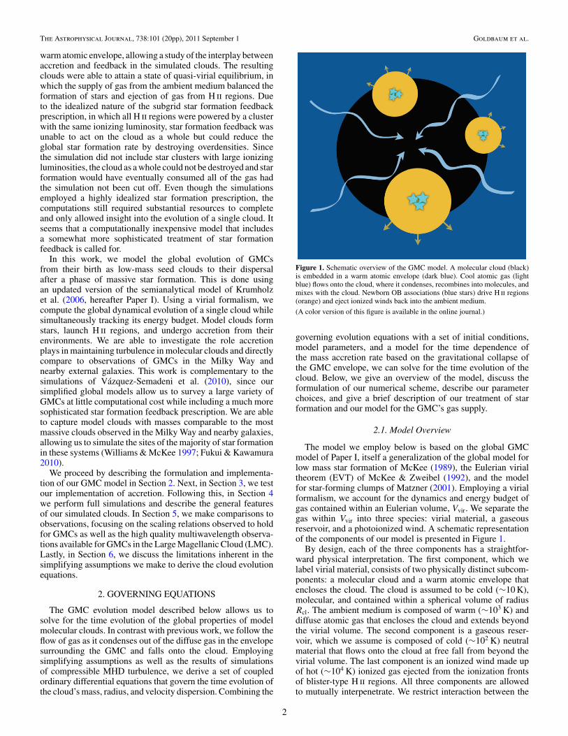
Figure 1. Schematic overview of the GMC model. A molecular cloud (black)is embedded in a warm atomic envelope (dark blue). Cool atomic gas (lightblue) flows onto the cloud, where it condenses, recombines into molecules, andmixes with the cloud. Newborn OB associations (blue stars) drive H ii regions(orange) and eject ionized winds back into the ambient medium.
(A color version of this figure is available in the online journal.)
governing evolution equations with a set of initial conditions,model parameters, and a model for the time dependence ofthe mass accretion rate based on the gravitational collapse ofthe GMC envelope, we can solve for the time evolution of thecloud. Below, we give an overview of the model, discuss theformulation of our numerical scheme, describe our parameterchoices, and give a brief description of our treatment of starformation and our model for the GMC’s gas supply.
2.1. Model Overview
The model we employ below is based on the global GMCmodel of Paper I, itself a generalization of the global model forlow mass star formation of McKee (1989), the Eulerian virialtheorem (EVT) of McKee & Zweibel (1992), and the modelfor star-forming clumps of Matzner (2001). Employing a virialformalism, we account for the dynamics and energy budget ofgas contained within an Eulerian volume, Vvir. We separate thegas within Vvir into three species: virial material, a gaseousreservoir, and a photoionized wind. A schematic representationof the components of our model is presented in Figure 1.
By design, each of the three components has a straightfor-ward physical interpretation. The first component, which welabel virial material, consists of two physically distinct subcom-ponents: a molecular cloud and a warm atomic envelope thatencloses the cloud. The cloud is assumed to be cold (∼10 K),molecular, and contained within a spherical volume of radiusRcl. The ambient medium is composed of warm (∼103 K) anddiffuse atomic gas that encloses the cloud and extends beyondthe virial volume. The second component is a gaseous reser-voir, which we assume is composed of cold (∼102 K) neutralmaterial that flows onto the cloud at free fall from beyond thevirial volume. The last component is an ionized wind made upof hot (∼104 K) ionized gas ejected from the ionization frontsof blister-type H ii regions. All three components are allowedto mutually interpenetrate. We restrict interaction between the
2

The Astrophysical Journal, 738:101 (20pp), 2011 September 1 Goldbaum et al.
components to the transfer of mass between the accretion flowand cloud as well as between the cloud and wind. Since the en-velope and cloud are not allowed to interpenetrate, we formallygroup the envelope and cloud together; this somewhat artificialchoice significantly simplifies the virial analysis.
We make use of two simplifying assumptions regarding thedistribution and flow of the virial material. First, we assume thatthe virial material follows a spherically symmetric, smoothlyvarying density profile. Second, we assume that the cloud ishomologous: the cloud expands, contracts, accretes, and shedsmass in such a way as to always maintain the same smoothdensity profile. We assume a density profile of the form
ρ(r) = ρ0
(r
Rcl
)−kρ
for r � Rcl, (1)
where ρ0 is the density at the edge of the cloud and kρ
is assumed to be unity. This choice is consistent with theLarson scaling relations observed in galactic (Larson 1981;Solomon et al. 1987; Heyer et al. 2001, 2009) and extragalactic(Mizuno et al. 2001; Engargiola et al. 2003; Rosolowsky 2007;Bolatto et al. 2008; Hughes et al. 2010) GMCs. Our assumedcloud density profile effectively averages over the clumpy andfilamentary internal structure and oblate shapes of observedclouds. At r = Rcl, the density of the ambient medium isassumed to smoothly transition from ρ0 to ρamb in a thinboundary layer. We assume that the density of the ambientmedium is negligible compared to the density of gas in thecloud, ρamb � ρ0. The density of the ambient medium remainsρamb out to the virial radius.
Beyond assuming a density profile, we must also specifythe velocity structure of all three components of the model. Wefollow Paper I in assuming that the velocity of the virial materialcan be decomposed into a systematic and turbulent component,
v = Rcl
Rclr + vturb. (2)
We assume that vturb is randomly oriented with respect toposition so that turbulent motions carry no net flux of matter.We make a similar assumption regarding the velocity structureof the reservoir,
vres = vres,sysr + vres,turb. (3)
The systematic component of vres is due to the gravitationalattraction of material within the virial volume
v2res,sys
2=
∫ r
∞g · dr, (4)
while the random component is such that (M−1cl
∫Vcl
ρv2res,turb
dV )1/2 = √3σres. Here, g is the gravitational acceleration
and σres is the velocity dispersion of gas in the reservoirfeeding the accretion flow. Since the amount of material inthe accretion flow is determined by how fast it can fall intothe cloud, we must simultaneously determine both the densityprofile and radial velocity of material in the accretion flow (seeAppendix B). Finally, for the wind material, we follow Paper Iin assuming
vw = v + v′ej, (5)
where v′ej = 2ciir and cii is the ionized gas sound speed. We
follow McKee & Williams (1997) in choosing cii = 9.7 km s−1.
2.2. Momentum Equation
In Appendix A, we derive the EVT for a simultaneouslyevaporating and accreting cloud,
1
2Icl = 2(T − T0) + B + W − 1
2
d
dt
∫Svir
(ρvr2) · dS
+ aIMclRclRcl +1
2aIMclR
2cl + aIMejRclRcl
+3 − kρ
4 − kρ
Rcl(Mejv′ej − ξMaccvesc). (6)
Here, aI is a constant of order unity that depends on thedistribution of material in the cloud, Icl is the cloud momentof inertia, T is the combined turbulent and thermal kineticenergy of the cloud, T0 is the energy associated with interstellarpressure at the cloud surface, B is the net magnetic energydue to the presence of the cloud, W is the gravitational term(equal to the gravitational binding energy in the absence of anexternal potential; McKee & Zweibel 1992), the surface integralis proportional to the rate of change of the moment of inertiainside the bounding viral surface, Mcl is the cloud mass, Rcl isthe cloud radius, Mej is the mass ejection rate, Macc is the massaccretion rate, vesc = {2G[Mcl +Mres(Rcl)]/Rcl}1/2 is the escapevelocity at the edge of the cloud, and ξ is a dimensionless factorwe compute via Equation (A8) that depends on the depth ofthe cloud potential well. The quantity ξvesc is the accretion rateweighted average infall velocity. Precise definitions for T , T0,B, and W are given in Paper I.
The EVT of a cloud without accretion or mass loss wouldonly contain the terms up to the surface integral. The next threeterms account for changes in the cloud moment of inertia due tochanges in the mass of the cloud, while the last term accountsfor the rate at which the recoil of inflowing and outflowingmass injects momentum into the cloud. Inflows and outflowsare treated separately because material is ejected at a constantvelocity, but is accreted at a velocity that is a function of thedepth of the potential well of the cloud. The dimensionless factorξ appears due to this difference.
The mass of the cloud can only change via mass accretion orejection,
Mcl = Mej + Macc. (7)
We assume that ejection of material can only decrease themass of the cloud and accretion can only increase the mass ofthe cloud. Since stars may not follow the homologous densityprofile we assume, we neglect the change in the cloud mass dueto star formation. We expect that the error incurred from thisassumption will be small, since stars make up a small fraction ofthe mass of observed clouds (Evans et al. 2009; Lada et al. 2010)and our assumed star formation law converts a small fraction ofthe cloud’s mass into stars per free-fall time.
We follow Paper I in using the assumption of homologyand the results of simulations of MHD turbulence to evaluateeach term in the EVT in terms of constants and the dynamicalvariables Rcl, Mcl, and σcl. In the end, we obtain a second-ordernonlinear ordinary differential equation in Rcl,
aIRcl = 3c2
cl
Rcl+ 3.9
σ 2cl
Rcl− 3
5a′(1 − η2
B
)GMcl
R2cl
− 4πPambR2
cl
Mcl
− aIMacc
MclRcl +
(3 − kρ
4 − kρ
) (Mej
Mclv′
ej − ξMacc
Mclvesc
).
(8)
3

The Astrophysical Journal, 738:101 (20pp), 2011 September 1 Goldbaum et al.
Here,
a′ = 15 − 5kρ
15 − 6kρ
[1 + (3 − 2kρ)
∫ 1
0x1−kρ y(x)dx
], (9)
y(x) is the ratio of the mass of reservoir material to the mass ofcloud material contained within a normalized radius x = r/Rcl(see Appendix B), and ηB is the ratio of the magnetic criticalmass to the cloud mass.
This equation governs the balance of forces acting on thecloud as a whole. Each term corresponds to a single physi-cal mechanism that can alter the radial force balance. The firsttwo terms are due to thermal and turbulent pressure support,respectively. The third is due to a combination of gravitationalcompression and magnetic support. The fourth is due to the con-fining interstellar pressure. The fifth comes from the exchangeof momentum between the expanding cloud and infalling accre-tion flow. Finally, the last term is due to a combination of therecoil from ejected material and the ram pressure of accretingmaterial. Although the two parts of the recoil term have oppo-site signs, Mej and Macc have opposite signs as well: Mej < 0and Macc > 0. This implies that both the recoil due to launch-ing wind material and the ram pressure of accreting reservoirmaterial tend to confine the cloud.
Letting Mcl,0, Rcl,0, and σcl,0 be the cloud mass, radius, andvelocity dispersion at t = 0 and defining the initial cloud crossingtime, tcr,0 = Rcl,0/σcl,0, we can define the dimensionlessvariables M = Mcl/Mcl,0, R = Rcl/Rcl,0, σ = σcl/σcl,0, andτ = t/tcr,0. Letting primes denote differentiation with respectto τ , we can write Equation (8) in dimensionless form
R′′ = 3.9σ 2 + 3M−20
aIR− ηG
a′MR2
− ηP
R2
M
− M ′accR
′
M+ ηE
M ′ej
M− ηA
ξM ′acc
(f MR)1/2, (10)
whereM0 = σcl,0/ccl (11)
is the initial turbulent Mach number and we define the dimen-sionless constants
ηG = 3(1 − η2
B
)aIαvir,0
(12)
ηP = 4πR3cl,0Pamb
aIMcl,0σ2cl,0
(13)
ηE =(
5 − kρ
4 − kρ
)v′
ej
σcl,0(14)
ηA =(
5 − kρ
4 − kρ
) (10
αvir,0
)1/2
, (15)
where
αvir,0 = 5σ 2cl,0Rcl,0
GMcl,0(16)
is the initial nonthermal virial parameter (Bertoldi & McKee1992). These constants are set by the ratios of various forcesacting on the initial state of the cloud. ηG is proportional to theratio of the initial magnetic forces to the initial gravitationalforce, and ηP , ηE , and ηA are the ratios of the ambientpressure force, the mass ejection recoil force, and the initial
accretion ram pressure force to the initial internal turbulentforces, respectively.
Comparing Equation (10) with the corresponding equationgiven in Paper I, we see that two new terms proportional to M ′
acchave appeared. In practice, we find that, of the two terms, theone proportional to ηA dominates, implying that the primarydirect impact of accretion on the radial force balance of thecloud is to provide a confining ram pressure. We will see in thenext section that accretion also increases the turbulent velocitydispersion, implying that the kinetic pressure term also increaseswhen accretion is included. The cloud radius is determined by abalance between kinetic pressure and a combination of gravity,accretion ram pressure, and wind recoil pressure. Thermalpressure support is negligible.
We also note that although the ambient pressure term is of thesame form as in Paper I, we assume an observationally motivatedvalue for the ambient pressure, Pamb/kB = 3 × 10⁴ K cm−3
(McKee 1999). This includes thermal and turbulent pressurebut neglects magnetic and cosmic ray pressure, since magneticfields and cosmic rays permeate both the cloud and the ambientinterstellar medium (ISM). We have also adjusted the ambientpressure upward by a factor of two because GMCs form inoverdense regions of the ISM where the hydrostatic pressureis higher than average. In Paper I, Pamb was chosen to beartificially high to ensure that the cloud would start its evolutionin hydrostatic equilibrium. This choice was made to accountfor the weight of the gaseous reservoir that was not explicitlyincluded. In practice, by choosing a lower value for Pamb, wefind that the ambient pressure term is subdominant for mostof the evolution of the cloud. This is expected, since we nowcorrectly account for the pressure of the reservoir through theterm proportional to ηA. Once accretion halts, the cloud is left outof pressure equilibrium and must expand to match the ambientpressure. This effect is seen most clearly in the second columnof Figure 3.
2.3. Energy Equation
In Appendix C, we derive the time evolution equation for thetotal energy of the cloud,
dEcl
dt= Mcl
Mcl
[Ecl +
(1 − η2
B
)W
] − 4πPambR2clRcl
+GMclMcl
Rclχ
(1 − MclRcl
MclRcl
)
+
(3 − kρ
4 − kρ
)Rcl(Mejv
′ej − ξMaccvesc)
+ ϕ
(3
2Maccσ
2res +
3
2Maccσ
2cl + γ Maccv
2esc
)− aIMaccR
2cl − 3Maccσ
2cl + Gcl − Lcl, (17)
where Gcl and Lcl are the rates of energy gain and loss due toH ii regions and turbulent dissipation, respectively, Ecl is the totalenergy due to the presence of the cloud (see Equation (C5)), σresis the velocity dispersion of material that is being accreted, χis given by Equation (C8), γ is given by Equation (C15), andϕ is a free parameter that sets the amount of energy availableto drive accretion driven turbulence. The parameter ϕ is theonly adjustable constant in our model that is not constrainedby the results of simulations or observations and must be tunedto reproduce the observed properties of clouds. The evolution
4

The Astrophysical Journal, 738:101 (20pp), 2011 September 1 Goldbaum et al.
of the cloud is very sensitive to ϕ and we justify our fiducialchoice, ϕ = 0.75, in Section 3.
Equation (17) governs the global energy budget of the cloud.Each term has a straightforward physical explanation. The term(Mcl/Mcl)Ecl is the rate of change of the cloud’s energy as massis advectively added to or carried away from the cloud. Similarly,(Mcl/Mcl)(1 − η2
B)W is the rate of change of the gravitationaland magnetic energy due to changes in the mass of the cloud.The next term is the rate at which external pressure doescompressional work on the cloud. This is followed by a termthat accounts for the gravitational work done on the cloud by thereservoir as the cloud expands and contracts. The following termrepresents the rate at which mass inflows, outflows, and externalthermal and turbulent pressure, respectively, do compressionalwork on the cloud. The next term, which is proportional toϕ, represents the rate of kinetic energy injection via stirringof turbulence by accreted material. This is followed by twoterms that are proportional to Macc, which account for the factthat in the frame comoving with the motions of material in thecloud, accreted material is moving at the transformed velocity,vres − v, different to the velocity of the reservoir material in therest frame, vres. Lastly, Gcl andLcl are the rate of energy injectionby star formation and the rate at which energy is radiated away,respectively.
Noting that turbulent motions carry no net radial flux of matterand recalling that we had set Bturb = 0.6Tturb, we may evaluateEquation (C5) and obtain for the total cloud energy,
Ecl = 1
2aIMclR
2cl + 2.4Mclσ
2cl +
3
2Mclc
2cl
−[
3
5a′ (1 − η2
B
)+ χ
]GM2
cl
Rcl. (18)
Taking the time derivative of this expression, substituting intoEquation (17), and nondimensionalizing as in Section 2.2 yieldsa time evolution equation for σ ,
4.8
aIσ ′ = −R′R′′
σ− ηG
MR′
R2σ− ηP
R2R′
Mσ+ ηE
M ′ejR
′
Mσ
− ηA
M ′accR
′
(MR)1/2σ− M ′
accR′2
Mσ− (3 − 1.5ϕ)M ′
accσ
aIM
+ ηD
ϕςM ′acc
Mσ+ ηI
ϕγM ′acc
f Rσ+G − LaIMσ
, (19)
where ς = σres/σres,0,
G − L = Rcl,0(Gcl − Lcl)
Mcl,0σ3cl,0
, (20)
and we define the constants,
ηD = 3σ 2res,0
2aIσ2cl,0
, (21)
ηI = 10
aIαvir,0. (22)
Here, ηD is proportional to the ratio of the initial turbulent kineticenergy in the reservoir and the initial turbulent kinetic energy inthe cloud and ηI is proportional to the ratio of the initial kineticenergy due to the infall of the reservoir to the initial turbulentkinetic energy of the cloud.
Since motions in GMCs are highly supersonic, the internalstructure of a typical cloud is characterized by strong shocks.Because clouds have short cooling timescales, the shockspresent throughout GMCs must be radiative. The braking ofturbulent motions via radiative shocks has been extensivelystudied in numerical simulations (see, e.g., Mac Low et al. 1998;Stone et al. 1998) in which the turbulent dissipation timescaleis found to be tdis = Eturb/E = kλin/σcl where k is a constant oforder unity and λin is the characteristic length scale of turbulentenergy injection. The simulations of Stone et al. (1998) givek = 0.48 and Eturb = 2.4Mclσ
2cl. Motivated by this result and
using a scaling argument given by Matzner (2002) and McKee(1989), we assume that the dimensionless rate of energy loss isgiven by
L = ηv
φin
Mσ 3
R. (23)
Here, ηv is a constant of order unity that depends on the natureof MHD turbulence in the cloud and we assume φin = λin/4Rcl.The factor of four in our expression for φin appears because thelargest wavelength mode supported by the cloud is λmax = 4Rcl,corresponding to net expansion or compression of the cloud. Wemake use of the simulations of Stone et al. (1998) to calibrate thisexpression. For the run most resembling real molecular clouds,we find ηv = 1.2. We follow Paper I in adopting φin = 1.0below. This is motivated by the results of Brunt et al. (2009)(but see also Ossenkopf & Mac Low 2002; Heyer & Brunt2004) who compared the velocity structure of observed clouds,where λin cannot be directly observed, with the velocity structureof simulated clouds, where λin is known a priori and foundλin � Rcl.
Comparing our velocity dispersion evolution equation(Equation (19)) to the corresponding equation given in PaperI, we see there are four new terms proportional to M ′
acc. Inpractice, we find that the primary effect of accretion on the en-ergy balance of the cloud is to increase the turbulent velocitydispersion via the terms proportional to ϕ. We will show inSection 4.2 that the velocity dispersion is set by a balance be-tween the decay of turbulence and energy injected by accretionand star formation.
2.4. Star Formation and H ii Regions
Star formation is able to influence the evolution of the cloudby ejecting mass and by injecting turbulent kinetic energy asexpanding H ii regions merge with and drive turbulent motionsin the cloud. The first mechanism is accounted for in our modelsby including an ionized wind that decreases the mass of the cloudand confines the cloud by supplying recoil pressure. The secondmechanism is accounted for by the Gcl term in Equation (17)which represents the injection of energy by H ii regions.
Since we only know the global properties of the cloud, wecalculate the rate of star formation by making use of a power-law fit to the star formation law of Krumholz & McKee (2005).Stars form at a low efficiency per free-fall time, consistentwith observations of star formation in nearby molecular clouds(Krumholz & Tan 2007). Individual star formation events occuronce a sufficient amount of mass has accumulated to form a starcluster. Star cluster masses are found by drawing from a clustermass function appropriate for a single cloud (see Equation (44)of Paper I). We then populate the cluster with individual stars bypicking masses from a Kroupa (2002) IMF. If the total ionizingluminosity of the newborn star cluster is sufficient to drive the
5

The Astrophysical Journal, 738:101 (20pp), 2011 September 1 Goldbaum et al.
expansion of an H ii region, we begin to track the resultingexpansion.
Once a massive star cluster forms, it photoionizes gas in itssurroundings and drives the expansion of an H ii region. Paper Itracked the expansion of individual H ii regions by assuming theanalytic self-similar solution for H ii region expansion workedout by Matzner (2002). This solution uses the fact that once anH ii region has expanded beyond the Stromgren radius, mostof the mass in the H ii region volume is in a thin shell ofatomic gas at a radius rsh from the center of the H ii region.The ionized gas in the interior of the shell exerts a pressure onthe surface of the shell, causing the shell to accelerate outward.The shell evolution equation derived from this analysis admitsa self-similar solution for the expansion of the H ii region. Thisself-similar result does a good job of predicting the expansionif there is no characteristic scale in the problem.
However, the introduction of radiation pressure leads to acharacteristic radius, rch, and time, tch. Radiation pressure is thedominant force driving the expansion of the ionized bubble whenrsh < rch and gas pressure dominates when rsh > rch. KM09modified the theory of Matzner (2002) to account for the effectof radiation pressure in the initial stages of the expansion. Theyderived an explicit functional form for rch and tch in terms of thebolometric and ionizing luminosity of the central star cluster,properties of the molecular cloud, and fundamental constants(see Equations (4) and (9) in KM09). The numerical value of rchand tch depends on the bolometric luminosity and the ionizingphoton flux of the central star cluster. The value we choose forftrap, a factor that accounts for the trapping and reradiation ofphotons as well as the trapping of main-sequence winds withinthe neutral shell, and φ, a factor that accounts for the absorptionof radiation by dust, are the fiducial values quoted by KM09.
Defining the dimensionless variables xsh = rsh/rch andτsh = t/tch, the equation of motion for the shell reduces to(KM09)
d
dτsh
(x2
shdxsh
dτsh
)= 1 + x
1/2sh . (24)
This assumes that gas in the neighborhood of the H ii regionfollows a density profile proportional to r−1, effectively placingthe H ii region in the center of the cloud. This accounts for thefact that H ii regions form in overdense regions of the cloud. Inpractice, we solve Equation (24) numerically to obtain xsh anddxsh/dτsh and thus rsh(t) and rsh(t).
In a gas pressure driven H ii region, the force exerted onthe expanding bubble is twice the recoil force photoionizedmaterial imparts on the cloud as it is ejected (Matzner 2002). Thephotoevaporation rate can then be straightforwardly calculatedvia Mej = −psh/2cii. Here, psh is the momentum of the shell andpsh is the force acting on the shell. In a radiation pressure drivenH ii region, the total force is given by the sum of the gas pressureand radiation pressure forces, psh = pgas + prad. At early times,when rsh � rch, the radiation force dominates, so prad pgas.Thus, if we calculate the mass ejection rate from the total forceacting on the shell, we will overestimate the mass ejection ratein a radiation pressure dominated H ii region. To correct for thiseffect, we modify the analysis of Paper I by only including thegas pressure force when we calculate the mass ejection rate,
Mej = − pgas
2cii
, (25)
where
pgas =(
12Sφπ
αB
)1/2
2.2kBTiir1/2sh (26)
= 3.3 × 1028L39 x1/2sh dynes. (27)
Since we do not include the dynamical ejection of material asH ii regions break out of the cloud surface, this is formally alower limit on the true mass ejection rate. Since clouds areclumpy and somewhat porous (Lopez et al. 2011), we expect tomake little error by neglecting dynamical ejection.
Once the stars providing 50% of the total ionizing luminosityof the central star cluster have left the main sequence, the H ii
region enters an undriven momentum-conserving snowplowphase. When the expansion velocity of the H ii region iscomparable to the turbulent velocity dispersion, we assume thatthe H ii region breaks up and contributes turbulent kinetic energyto the cloud. H ii regions can merge with the cloud during eitherthe driven or undriven phases. If the radius of the H ii region isgreater than the radius of the cloud and the expansion velocityof the shell is greater than the cloud escape velocity, we say theH ii region disrupts the cloud and end the global evolution.
If an H ii region merges with the cloud at time t = tm whenits radius is rsh = rm, the rate of energy injection from a singleH ii region is given by
Gcl = 1.6ηET1(tm)
(rm
Rcl
)1/2
δ(t − tm). (28)
Here T1(tm) = pshσcl/2, ηE parameterizes the efficiency ofenergy injection, δ(t) is the Dirac delta function, and thefactor of 1.6 arises because magnetic turbulence is slightlysub-equipartition compared to kinetic turbulence. The factor(rm/Rcl)1/2 accounts for the more rapid decay of turbulencewhen the driving scale is smaller (see Paper I).
2.5. Mass Accretion
Consistent with the analysis in Appendix B, we treat thereservoir as a gravitationally unstable spherical cloud undergo-ing collapse. The cloud is primarily composed of atomic gasin both warm and cold phases. We expect that as the reservoircollapses, material that is accreted onto the cloud will cool andbecome molecular. We approximate that the reservoir has ap-proximately constant surface density, Σres. To find an upper limiton the mass accretion rate, we can assume that the reservoir isundergoing collapse in the limit of zero pressure. It is straight-forward to show that the resulting accretion rate onto the centralcondensation is given by
Macc,ff = 256
πG2Σ3
rest3. (29)
Since the estimate for the accretion rate given in Equation (29)does not take into account pressure support, it is likely anoverestimate of the true accretion rate. Indeed, McKee &Tan (2003) considered the inside out collapse of equilibriumpolytropic molecular cloud cores and, in the case of kρ = 1,found the same scaling with time and surface density but asubstantially lower coefficient. Tan & McKee (2004) arguedthat subsonic inflow was a more realistic initial condition thanthe static equilibrium solution used by McKee & Tan (2003).Hunter (1977) found the set of solutions for the collapse of anisothermal sphere starting at an infinite time in the past. The
6

The Astrophysical Journal, 738:101 (20pp), 2011 September 1 Goldbaum et al.
solution with an infall velocity of about ccl/3 corresponds wellto the results of the simulation of the formation of a primordialstar by Abel et al. (2002). Tan & McKee (2004) adopted thissolution, noting that it has an accretion rate that is 2.6 timesgreater than that for a static initial condition (Shu 1977) whenexpressed in dimensionless form. Our problem is quite differentfrom Hunter’s, since an equilibrium density gradient kρ = 1corresponds to γ = 0 (McKee & Tan 2003) rather than Hunter’sγ = 1. Nonetheless, we assume that the accretion rate for ourproblem is also 2.6 times greater than that for a static initialcondition and find
Macc,TM04 = 10.9 G2Σ3rest
3. (30)
Clearly, this result is uncertain, and magnetic fields introducefurther uncertainty. Fortunately, we find that varying the numer-ical coefficient in Equation (30) does not affect the qualitativenature of the results discussed below.
To model the effect of a finite gas supply, once the total massof gas that has fallen onto the cloud exceeds the total mass ofthe reservoir, Mres, we set Macc = 0. When comparing withgalactic populations of GMCs, we set Mres = 6 × 10⁶ M�,the observed upper mass cutoff for GMCs (Williams & McKee1997; Fukui & Kawamura 2010). This may underestimate thetrue upper mass since fragmentation may lead to a range ofreservoir masses. Since 6 × 10⁶ M� GMCs are relatively rare,we set Mres = 2 × 10⁶ M� for the runs presented in Figure 3and Table 2 as ∼106 M� is a more typical GMC mass.
If we also assume that the atomic reservoir is such that thevirial parameter of the reservoir, αres, is constant with radius,we find
σres = 0.4α1/2res GΣrest. (31)
Fiducially, we take αres = 2.0, corresponding to a marginallygravitationally bound reservoir. This parameterization assumesthat the reservoir satisfies an internal linewidth–size relationof the form σres(r) ∝ r1/2. The increase of the reservoirvelocity dispersion with time reflects that material originatesat increasingly larger radii.
The precise normalization of the mass accretion law is amajor source of uncertainty in our modeling. Since the lengthscales over which material is swept up into the cloud throughthe reservoir approach galactic dynamical scales (Dobbs et al.2011; Tasker 2011), a more complete treatment would requiretracking the gas dynamics from the scale of an entire galaxydown to the scale of the reservoir. This would also allow usto self-consistently model the end of accretion onto the cloudinstead of assuming that mass accretion cuts off abruptly. In aforthcoming paper, we plan to add our molecular cloud modelsto a simulation of gas dynamics in a galactic disk to model thegas reservoir for a population of GMCs.
Although the normalization of the accretion law is somewhatuncertain, we can make use of observations of the gas content ofnearby galaxies to estimate Σres, the surface density of gas in thereservoir feeding the cloud. The average H i surface density inthe inner disk of the Milky Way is observed to be approximatelyconstant, ∼8 M� pc−2 (Kalberla & Dedes 2008). Beyond agalactocentric radius of ∼10–15 kpc, the H i surface densitydecreases exponentially with radius; however, few GMCs areobserved in the outer Milky Way (Heyer et al. 2001) or beyondthe optical radius of nearby galaxies (Engargiola et al. 2003;Bigiel et al. 2008). Similar saturated mean H i surface densitiesare observed in nearby galaxies, except in the central regionsof some galaxies where the ISM becomes fully molecular and
the H i surface density goes to zero (Leroy et al. 2008). Forthis reason, we adopt Σres = 8 M� pc−2 as a fiducial atomicreservoir surface density typical of the bulk ISM of local star-forming galaxies.
Although the mean atomic surface density in nearby galaxiesis as low as 8 M� pc−2, the atomic ISM is observed to be clumpy,with overdense regions reaching significantly higher surfacedensities. These regions may be associated with spiral arms,as in M 33 (Thilker et al. 2002), or driven by gravitationalinstability, as in the LMC (Yang et al. 2007). For this reason, wealso explore the behavior of molecular clouds accreting fromhigher surface density gas, Σres = 16 M� pc−2. Since massivemolecular clouds are universally observed to be associated withhigh surface density gas (Wong et al. 2009; Imara et al. 2011), weexpect there to be marked differences between molecular cloudsthat accrete from high surface density gas and clouds that accretefrom low surface density gas. Although the gas will be primarilyatomic at a gas surface density of 16 M� pc−2, we expect thatthere should be some diffuse “dark” molecular gas (Krumholzet al. 2008; Wolfire et al. 2010). Thus, the reservoir is notnecessarily completely atomic, but instead primarily composedof atomic gas.
2.6. Numerical Scheme
Equations (7), (10), and (19) constitute a system of coupled,stochastic, nonlinear ordinary differential equations in M, σ , andR. We solve these equations by using a straightforward Eulerintegration with an adaptive step size. The precise order in whichwe update cloud properties is as follows. After calculating theinstantaneous star formation rate, we calculate M ′ by summingthe components due to ionized winds and mass accretion. Next,we calculate the rate of turbulent dissipation using Equation(23). We then calculate ζ , the ratio of the mass doubling timeto the free-fall time, using Equation (B5). We use ζ to calculatea′, f, and ξ by interpolating on precomputed tables. Since σ ′depends on R′′, we first evaluate R′′ using Equation (10) andthen compute σ ′ using Equation (19). Next, we check if R, M,or σ will change by more that 0.1% using the current value ofthe time step. If we detect a change larger than this, the timestep is iteratively recalculated using a new time step half thesize of the original until the fractional changes in R, M, and σare smaller than 0.1%. Next, we calculate R, M, and σ at thenew time step, update the state of any H ii regions created inprevious time steps, and then create new H ii regions using theprocedure described in Section 2.4. If the time step did not needto be reduced, we increase the size of the time step by 10%.
Cloud evolution can be terminated if one of three conditionsis satisfied.
1. The time step is less than 10−8 of the current evolution time(i.e., Δτ/τ < 10−8).
2. The mean visual extinction falls below AV,min = 1.4,corresponding to the CO dissociation threshold found byvan Dishoeck & Black (1988).
3. An H ii region envelops and unbinds the cloud, i.e., ifrsh > Rcl and rsh > vesc.
We use the phrases collapse, dissociation, and disruption, re-spectively, to describe these scenarios. The dissociation thresh-old depends on the ambient radiation field. However, Wolfireet al. (2010) found that the CO dissociation threshold varies byonly a factor of two when the intensity of the ambient radiationfield varies by an order of magnitude, so we neglect variationsin the radiation field and, for consistency with Paper I, adopt
7

The Astrophysical Journal, 738:101 (20pp), 2011 September 1 Goldbaum et al.
Table 1Fiducial Parameters
Parameter Value Reference
αvir,0 2.0 Blitz et al. (2007)Σcl,0 60 M� pc−2 Heyer et al. (2009)cs
a 0.19 km s−1 . . .
cii
b 9.74 km s−1 McKee & Williams (1997)ηB 0.5 Krumholz & McKee (2005)ηE 1.0 Paper Iηv 1.2 Paper Iφin 1.0 Brunt et al. (2009)ϕ 0.75 This workAV,min 1.4 van Dishoeck & Black (1988)αres 2.0 . . .
Pamb/kB 3 × 10⁴ K cm−3 McKee (1999)Mcl,0 5 × 10⁴ M� . . .
Notes.a Assumes T = 10 K and μ = 2.3.b Assumes T = 7000 K and μ = 0.61.
AV,min = 1.4. The surface density corresponding to the disso-ciation threshold depends on the assumed dust to gas ratio andthus on the metallicity. For solar metallicity, a surface density of1 g cm−2 corresponds to AV = 214.3. Since we use a dissocia-tion threshold based on CO rather than H2 to define the end ofthe cloud’s life, we may miss the further evolution of a diffusemolecular cloud where most of the carbon is neutral or singlyionized but the hydrogen is still molecular.
These halting conditions probably oversimplify the true endof a cloud’s evolution due to our assumption of sphericalsymmetry and homology. For the case of collapse, it is morelikely that the cloud would undergo runaway fragmentationrather than monolithic collapse. In the case of dissociation,even if the mean surface density drops below the point whereCO can no longer remain molecular, that does not precludethe possibility that overdense clumps might retain significantamounts of CO. Finally, for the case of disruption, even if an H ii
region delivered a large enough impulse to unbind the cloud, itmay simply be displaced as a whole, or be disrupted into multiplepieces which would then evolve independently. It is also likelythat if the cloud is disrupted while still actively accreting, thecloud would inevitably recollapse since it is unlikely that anH ii region would have enough kinetic energy to unbind thereservoir.
Since we must necessarily use simple criteria to halt the cloudevolution, our estimates of cloud lifetimes presented below arestrictly lower limits to the true lifetime of a cloud. Both thedisruption and dissociation criteria do not preclude the presenceof overdense clumps that may survive the destruction events.However, our estimates of cloud lifetimes are appropriate for thelifetime of a single monolithic cloud. Any overdense clumps thatdo survive would represent entirely different clouds that wouldevolve independently of each other.
2.7. Input Parameters
To complete our model, we must choose a set of parametersand initial conditions to fully determine our cloud evolutionequations. In Table 1, we have listed the various fiducialparameters we have chosen for our model as well as thereferences from which we derive our choices. Some of theseparameters are motivated by observations, others by the resultsof simulations, and one parameter (ϕ, see Section 3) is left free.
The cloud initial conditions can be computed given an initialcloud mass along with our assumed value for αvir,0 and Σcl,0.Matzner & McKee (2000) and Fall et al. (2010) found thatprotostellar outflows are energetically important when Mcl �104.5 M�. Above this mass, they contribute negligibly. Thus,if we choose a low initial mass, we may be underestimatingthe amount of turbulent energy injection by star formationfeedback at early times since we do not account for protostellaroutflows. For this reason, we choose a relatively large initialmass, Mcl,0 = 5 × 10⁴ M�. For reference, given our choice ofinitial virial parameter and surface density, this corresponds toRcl,0 = 11.5 pc, σcl,0 = 2.7 km s−1, and tcr,0 = 4.1 Myr. Whilethis is larger than some local molecular clouds like Taurus orPerseus, it is still much smaller than the mass of the molecularclouds where most of the star formation in local galaxies occurs.
3. MODELS WITH ACCRETION ONLY
Before beginning full simulations using our method, we mustfirst test the behavior of our model as we vary the free parameterϕ introduced in the derivation of the energy evolution equation.For this purpose, we have run our model with star formationfeedback disabled. The only physical mechanisms modeled inthese tests are accretion and the decay of turbulence. Since thereis no random drawing from the stellar or cluster IMF in theseruns, the results are fully deterministic. These simplified modelsallow us to understand how the results depend on our choice forthe tunable parameter ϕ and provide physical insight that willbe useful in interpreting the results of the more complex andstochastic runs that include feedback.
The energetics and virial balance of our cloud models dependcritically on the parameter ϕ. Broadly speaking, ϕ controls theamount of turbulent kinetic energy injected by the accretionflow. For the case ϕ = 0 the accretion flow contributes theminimum possible amount of turbulent kinetic energy. Thismeans that accreted material cannot contribute significantlyto turbulent pressure support, since the accreted material ismaximally subvirial. With this choice, as the cloud accretesmass, its energy budget must become increasingly dominatedby self-gravity. Once this happens, internal pressure support isnegligible and the cloud must inevitably undergo gravitationalcollapse.
Alternatively, we could set ϕ > 0. If ϕ is small, the turbulentkinetic energy of a newly accreted parcel of gas would still besmall compared to the gravitational potential energy of the gasparcel. Thus, once the cloud is primarily composed of accretedgas, the cloud will undergo gravitational collapse, although ona slightly longer timescale than in the ϕ = 0 case. At somelarger value of ϕ, accretion contributes a net positive amountof energy to the cloud, balancing out the negative gravitationalpotential energy of the newly accreted material. The cloud willstill collapse with this choice since turbulent motions quicklydecay away. As ϕ is increased further, we should eventually findthat at some critical value, ϕ = ϕcrit, accretion drives turbulentmotions with sufficient vigor to avoid the gravitational collapseof the cloud entirely.
The results of test runs with different choices of ϕ arepresented in Figure 2. The time evolution of the cloud surfacedensity, virial parameter, velocity dispersion, and cloud radiusis plotted for a selection of clouds evolved with different choicesfor ϕ. Each line depicts the time evolution of a cloud propertyand is color coded by the value of ϕ chosen. It is obvious thatthe value of ϕ can strongly influence the resulting evolution.
8

The Astrophysical Journal, 738:101 (20pp), 2011 September 1 Goldbaum et al.
Figure 2. Cloud surface densities (bottom row), virial parameters (second row),velocity dispersions (third row), and radii (top row) for 400 different runs, eachwith a different choices for ϕ, as indicated in the color bar. Star formation wasturned off for all runs.
(A color version of this figure is available in the online journal.)
If ϕ = 0, the cloud experiences global collapse in a free-fall time. Initially, the cloud velocity dispersion decreases,but inevitably the gravitational term in the velocity dispersionevolution equation, proportional to −R′/R2, becomes dominant,and the velocity dispersion begins to diverge. The fact that σcldiverges as Rcl goes to zero is an artifact. In reality, the highestdensity regions would independently fragment and collapse andthe cloud would never undergo a monolithic collapse.
As we increase ϕ, the cloud is able to support itself againstcollapse for longer periods. Near ϕ = 0.5, accretion brings innet positive energy but turbulent dissipation wins out, and thecloud still eventually collapses. At a critical value, ϕcrit � 0.8,accretion driven turbulence alone is sufficient to hold up thecloud against collapse for as long as the reservoir continuesto supply mass to the cloud. The mass, radius, and velocitydispersion of the cloud increase in such a way as to maintain aconstant virial parameter and surface density.
Since we expect that gas motions driven by accreting denseclumps should be at least somewhat correlated with the motionsof the infalling clumps, we do not expect a physically realisticchoice of ϕ to be very close to zero. On the other hand, amodel in which a cloud is entirely supported by accretion driventurbulence seems to preclude the possibility that a significantfraction of the kinetic energy of infalling gas is radiated awayin an accretion shock. For this reason, we rule out as unphysicalruns with ϕ ≈ 0 and ϕ � ϕcrit. The precise value of ϕ we willuse in our models that include star formation below dependson uncertain details of the accretion and mixing of infallinggas. In practice, we find that even with the energy providedby star formation feedback, clouds generally undergo free-fallcollapse or reach unreasonably high mean surface densities oncethey are primarily composed of accreted material if we chooseϕ � 0.7. Since clouds are generally not observed to be in globalfree-fall collapse, we instead pick a value somewhat higherthat this, ϕ = 0.75, for our fiducial models. This splits thedifference between accretion contributing a negligible amountof energy to the cloud when ϕ = 0.5 and accretion contributing
the maximum possible amount of energy when ϕ = 1. Wewill see below that our fiducial choice broadly reproduces theobserved properties of molecular clouds in the Milky Way andnearby galaxies.
4. MODELS WITH ACCRETION AND STAR FORMATION
Feedback by the action of ionizing radiation emitted bynewborn stellar associations alters the evolution of a GMCafter the birth of the first massive star cluster. The source ofenergy provided by massive star formation can be a significantcomponent of the energy budget of the entire cloud. For theremainder of this paper, we consider models with the starformation prescription described in Section 2.4 turned on.
4.1. Overview of Results
We have run two sets of simulations with parameters chosen tomodel conditions in interarm (Σres = 8 M� pc−2) and spiral arm(Σres = 16 M� pc−2) regions. Besides the two different choicesfor the ambient surface density, all other parameters and initialconditions are identical. The time evolution of a subsample ofruns is plotted in Figure 3 and average properties of the fullsample are presented in Table 2.
The most striking result of our comparison is that the finalmass of our model molecular clouds depends on the assumedmass accretion history. Clouds evolved with a low accretionrate, corresponding to conditions in interarm regions, growlarger than 105 M� less than 30% of the time and very rarelyreach masses comparable to the most massive GMCs in theLocal Group. The vast majority of clouds are instead disruptedby an energetic H ii region within a few crossing times. Theclouds attain a quasi-equilibrium configuration in which massaccretion is roughly balanced by mass ejection. Clouds avoidglobal collapse by extracting energy from the expansion of H ii
regions.The evolution of the clouds is characterized by discrete energy
injection events due to the formation of a single massive starcluster. Once a cluster forms, it ejects a wind and launches anH ii region. The recoil force of launching the wind leads to anoverall confining ram pressure, causing the radius to decreaseand the surface density to increase. Once the star cluster burnsout, the H ii region expansion decelerates and then stalls. Whenthe expansion velocity of the H ii region is comparable to thecloud velocity dispersion, the kinetic energy of the expandingH ii region is converted into turbulent kinetic energy, causing aspike in the turbulent velocity dispersion. The turbulent kineticenergy exponentially decays away over a crossing time, but thetemporarily elevated velocity dispersion increases the turbulentkinetic pressure, causing the cloud to expand. This leads tooscillations in the cloud radius and mean surface density. Onthe whole, clouds that are not quickly disrupted by H ii regionsare able to survive as quasi-virialized objects for several crossingtimes before they are either disrupted or dissociated.
Clouds evolved with a higher ambient surface density, typicalof spiral arm regions in the Milky Way, exhibit significantlydifferent behavior. Since these clouds accrete mass much fasterthan in the low surface density runs, they are not able toattain steady state between accretion and ejection of mass.While some clouds are still destroyed by energetic H ii regionsearly in their evolution, over 90% of these clouds were ableto accrete their entire reservoir after 25 Myr. At this point,the clouds are generally quite massive, ∼1.5 × 10⁶ M�. Onceaccretion is shut off, the clouds are no longer confined by
9
The Astrophysical Journal, 738:101 (20pp), 2011 September 1 Goldbaum et al.
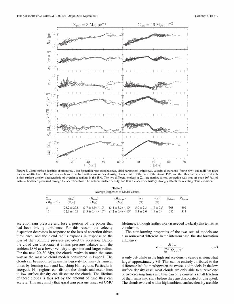
Figure 3. Cloud surface densities (bottom row), star formation rates (second row), virial parameters (third row), velocity dispersions (fourth row), and radii (top row)for a set of 40 clouds. Half of the clouds were evolved with a low surface density, characteristic of the bulk of the atomic ISM, and the other half were evolved witha high surface density, characteristic of overdense regions in the ISM. The two different choices of Σres are marked at top. Accretion was shut off once 106 M� ofmaterial had been processed through the accretion flow. The ambient surface density, and thus the accretion history, strongly affects the resulting cloud evolution.
Table 2Average Properties of Model Clouds
Σres 〈tlife〉 〈Mmax〉 〈Mejected〉 〈ε〉 〈εff〉 Ndissoc Ndisrupt
(M� pc−2) (Myr) (M�) (M�) (%) (%)
8 26.2 ± 29.8 (3.7 ± 4.9) × 105 (3.4 ± 5.3) × 105 5.0 ± 2.3 1.9 ± 0.5 308 69216 52.6 ± 16.8 (1.3 ± 0.4) × 106 (1.2 ± 0.4) × 106 8.3 ± 2.0 1.9 ± 0.4 687 313
accretion ram pressure and lose a portion of the power thathad been driving turbulence. For this reason, the velocitydispersion decreases in response to the loss of accretion driventurbulence, and the cloud radius expands in response to theloss of the confining pressure provided by accretion. Beforethe cloud can dissociate, it attains pressure balance with theambient ISM at a lower velocity dispersion and larger radius.For the next 20–30 Myr, the clouds evolve in much the sameway as the massive cloud models considered in Paper I. Theclouds can be supported against self-gravity for many dynamicaltimes by forming stars and launching H ii regions. Particularlyenergetic H ii regions can disrupt the clouds and excursionsto low surface density can dissociate the clouds. The lifetimeof these clouds is thus set by the amount of time they canaccrete. This may imply that spiral arm passage times set GMC
lifetimes, although further work is needed to clarify this tentativeconclusion.
The star-forming properties of the two sets of models arealso somewhat different. In the interarm case, the star formationefficiency,
ε = M∗,tot∫ tlife0 Maccdt
, (32)
is only 5% while in the high surface density case, ε is somewhatlarger, approximately 8%. This can be entirely attributed to thedifference in lifetimes between the two sets of models. In the lowsurface density case, most clouds are only able to survive oneor two crossing times and thus can only convert a small fractionof their mass into stars before they are dissociated or disrupted.The clouds evolved with a high ambient surface density are able
10

The Astrophysical Journal, 738:101 (20pp), 2011 September 1 Goldbaum et al.
Figure 4. Number of clouds plotted as a function of |EH ii/Eacc|. In regions of low ambient surface density, accretion and star formation are in equipartition, while inregions of high ambient surface density, accretion dominates the energy budget.
(A color version of this figure is available in the online journal.)
to survive for many crossing times and convert a larger fractionof their gas into stars. An even larger fraction is ejected viaphotoionization. However, for both models, the star formationefficiency per free-fall time,
εff = M∗Mcltff
, (33)
is low, around 2%. This is not surprising, as a low star formationefficiency per free-fall time is one of the basic assumptions ofour model.
4.2. Energetics of Star Formation FeedbackVersus Mass Accretion
GMCs exhibit highly supersonic turbulence. There is noagreement in the literature about what drives these motions,which numerical models of compressible MHD turbulenceindicate should decay if left undriven. Some authors suggest thatthe primary energy injection mechanism is some sort of internalstar formation feedback process, such as protostellar outflows(Li & Nakamura 2006; Wang et al. 2010), expanding H ii regions(Matzner 2002), or supernovae (Mac Low & Klessen 2004).Others suggest that turbulence is driven externally via massinflows (Klessen & Hennebelle 2010). Comparing the amountof energy injected by different forms of star formation feedback,Fall et al. (2010) found that at typical GMC column densities,the dominant stellar feedback mechanism is H ii regions drivenby the intense radiation fields emitted by massive star clusters.Using our models, we can compare the importance of accretionrelative to H ii regions in the energy budget of GMCs.
To find the total energy injected by accretion, we make use ofour knowledge of the total energy of the cloud as a function oftime. At the end of time step j we use Equation (18) to calculateboth the total cloud energy, Ecl,j , as well as what the cloudenergy would have been if we had set Macc = 0 for that timestep, Ecl|Macc=0. The difference,
Eacc,j = Ecl,j − Ecl|Macc=0, (34)
is the total energy added by accretion during that time step. Thetotal energy injected by accretion over the cloud’s lifetime is
just the sum of the contributions of each time step,
Eacc =∑
j
Eacc,j . (35)
The energy injected by H ii region i, EH ii,i , can be found byintegrating the rate of energy injection by a single H ii regionwith respect to time. This is,
EH ii,i = 1.6ηET1,i
(rm,i
Rcl,i
)1/2
, (36)
where rm,i is the radius of H ii region i when it merges with theparent cloud and Rcl,i is the radius of the cloud as a whole whenH ii region i merged with the cloud. To find the total energyinjected by H ii regions over the cloud’s lifetime, we simplysum up the contributions due to individual H ii regions,
EH ii =∑
i
EH ii,i . (37)
The ratio |EH ii/Eacc| indicates the relative importance ofstar formation feedback to accretion driven turbulence to theglobal energy budget of the cloud. If |EH ii/Eacc| < 1, accretiondominates the energy injection; similarly if |EH ii/Eacc| > 1, starformation feedback is the primary driver of turbulence.
The results of this comparison are plotted for both choices ofthe ambient surface density in Figure 4. We find that H ii regionsand accretion contribute approximately equal amounts of energyin the low surface density runs, while accretion dominates inthe high surface density runs. In the low surface density runs,stochastic effects can be important, particularly for clouds thatdo not last much longer than a crossing time. Thus, in someruns, star formation feedback can contribute significantly moreenergy than accretion, while in others star formation feedbackis negligible. In the runs evolved with a high ambient surfacedensity, star formation feedback is subdominant, although notcompletely negligible, in the vast majority of runs.
It is worth pointing out that this result depends on theprecise value of ϕ we choose to evolve the clouds with. If ϕis lower, accretion contributes less energy, and star formationcan dominate the energy budget. If ϕ is higher, star formation
11

The Astrophysical Journal, 738:101 (20pp), 2011 September 1 Goldbaum et al.
becomes completely negligible, and the amount of kineticenergy injection is controlled by the mass accretion rate. Sinceclouds collapse when we choose ϕ much lower than ourfiducial value, and shocks in molecular gas tend to be stronglydissipative, we do not expect the “true” value of ϕ to be muchdifferent than our fiducial value. We thus conclude that one ofthree cases must hold. Star formation may be dominant, but onlymarginally so. Accretion may also be dominant, but again, onlymarginally. It is also possible that star formation and accretioncontribute roughly equal amounts of energy. In all three cases,neither star formation or accretion is truly negligible.
5. OBSERVATIONAL COMPARISONS
5.1. Larson’s Laws
GMCs are observed to obey three scaling relations, known asLarson’s laws (Larson 1981; Solomon et al. 1987; Bolatto et al.2008). In their simplest form, Larson’s laws state the following.
1. The velocity dispersion scales with a power of the size ofthe cloud. Subsequent observations have shown that thispower is about 0.5 (σcl ∝ R0.5
cl ).2. The mass of the cloud scales with the square of the radius
(constant Σcl).3. Clouds are in approximate virial equilibrium (αvir of order
unity).
These laws are not independent; any two imply the other. Ata minimum, an acceptable theoretical model for GMCs shouldagree with both the scaling and the normalization of the Larsonscaling relations observed in real clouds. We have already seenthat clouds maintain approximate virial equilibrium as wellas roughly constant surface densities, but we have yet to seewhether the normalization of the Larson scaling relations forour models agrees with the observed Larson scaling relations.
5.1.1. Equilibrium Surface Densities
GMCs, both in the Milky Way (Larson 1981; Solomon et al.1987) and in nearby external galaxies (Blitz et al. 2007; Bolattoet al. 2008), exhibit surprisingly little variation in surfacedensity. For the Solomon et al. (1987) sample of Milky Wayclouds, this was found to be 〈Σcl〉 = 170 M� pc−2. Morerecent and sensitive observations find lower values, closer to〈Σcl〉 = 50 M� pc−2, in the Milky Way (Heyer et al. 2009)and in the LMC (Hughes et al. 2010), although these latterestimates depend on a highly uncertain correction for non-LTEline excitation and the CO to H2 conversion factor, respectively.Using heterogenous data from several nearby galaxies, Bolattoet al. (2008) attempted to extract cloud properties in a uniformmanner and found a typical surface density of 85 M� pc−2 butwith significant variation from galaxy to galaxy.
Variations in the mean GMC surface density are seen whencomparing samples from different galaxies. However, within asingle galaxy there is little variation (Blitz et al. 2007). Thesevariations are usually attributed to differences in the CO-to-H2conversion factor from galaxy to galaxy (Bolatto et al. 2008),a quantity which may depend on metallicity and the interstellarradiation field (Glover et al. 2010) as well as variations inturbulent pressure and radiation field in the ambient ISM. Inour runs, we also recover roughly constant surface densities(see the second row from the bottom of Figure 3).
In Figure 5, we have reproduced a figure from Blitz et al.(2007) that depicts observational results for CO luminositiesand cloud radii for a sample of clouds in the outer Milky Way
l
l
l
Figure 5. Cloud CO luminosity plotted as a function of cloud radius. COluminosities are found by assuming XCO = 4×1020 cm−2 (K km s−1)−1. Solidlines of constant surface density are plotted for 10, 100, and 1000 M� pc−2
for reference. The dashed line of constant surface density corresponds to ourassumed dissociation threshold. The outputs from a set of 2000 runs were used,with Σres = 8 and 16 M� pc−2 and Mres = 6 × 10⁶ M�. Colors indicate theamount of time model clouds tend to occupy a position in LCO–Rcl parameterspace. Symbols denote observed CO luminosities and cloud radii for galactic(points) and extragalactic (open shapes) GMCs. See Blitz et al. (2007) andreferences therein for details of the observations.
(A color version of this figure is available in the online journal.)
as well as from several samples of extragalactic GMCs. Tocompare against this compendium of results, we calculate COluminosities for our model clouds by assuming a constant CO-to-H2 conversion factor,
LCO = Mcl
8.8 M�K km s−1 pc2 (38)
as in Rosolowsky & Leroy (2006). This formula accountsfor the presence of helium and assumes a constant H2-to-COconversion factor, XCO = 4 × 1020 cm−2 (K km s−1)−1, twicethe value derived for molecular clouds within the Solar circleusing observations of gamma-ray emission (Strong & Mattox1996; Abdo et al. 2010). We choose this value to be consistentwith Blitz et al. (2007), who find, using this value of XCO, thatall of the GMCs in their sample have virial masses comparableto the masses implied by their CO luminosity to within a factorof two.
With our fiducial initial conditions, model clouds in oursample begin their lives in the bottom left-hand corner ofFigure 5 at Rcl ≈ 10 pc. As they accrete and expand, cloudsmove toward the upper right-hand corner. Clouds end theirevolution either through disruption by a single H ii region or bypassing below the molecular dissociation threshold, indicatedby a dashed line in Figure 5. Offsets in the distribution ofcolumn densities from galaxy to galaxy and from the simulatedclouds can be attributed to variations in XCO and uncertaintyin identifying a unique radius for observed clouds (Blitz et al.2007) that have nonzero obliquity (Bertoldi & McKee 1992).Accounting for variations in XCO, there is striking agreementbetween the observed distribution of molecular clouds and oursample of simulated clouds.
The models exhibit a kink in their evolution when the reservoiris exhausted and accretion is shut off. For this reason, thereare no clouds with LCO > 105.6 K km s−1 pc2. Once accretion
12

The Astrophysical Journal, 738:101 (20pp), 2011 September 1 Goldbaum et al.
l
l
l
Figure 6. Cloud velocity dispersion plotted as a function of cloud radius. Thedash-dotted line is the galactic linewidth–size relation found by Solomon et al.(1987), σv = 0.72R0.5. Symbols and color coding are the same as in Figure 5.
(A color version of this figure is available in the online journal.)
is shut off, the clouds decrease in mass for the remainder oftheir evolution. This kink is somewhat artificial since we haveassumed a fixed reservoir mass and a smooth accretion history.A more sophisticated model for the reservoir including a rangeof reservoir masses would exhibit a continuous spectrum ofkinks, broadening the region of parameter space explored bythe models, particularly for LCO < 104.5 K km s−1 pc2.
The models also exhibit two distinct favored strips of param-eter space along which they tend to evolve. This correspondsto the two different equilibrium column densities picked out bythe two different choices of Σres. This behavior is clearly seenin the second panel from the bottom of Figure 3. The fact thatΣcl is sensitive to Σres follows from dimensional analysis.
5.1.2. Linewidth–Size Relation
We next compare our simulated clouds with thelinewidth–size relation observed to hold among GMCs as a pop-ulation (Bolatto et al. 2008). In Figure 6, we plot the region ofvelocity dispersion–size parameter space explored by our cloudmodels, along with the observed velocity dispersions and sizesfor a selection of Local Group GMCs. We are able to reproducethe power law, scatter, and the rough normalization in the ob-served linewidth–size relation. This conclusion is unsurprising,since we have already seen that our simulated clouds maintainroughly constant virial parameters and surface densities as theyevolve. It is worth noting that, for our simplified model for theenvironment of a GMC, the linewidth–size relation correspondsto an age sequence. Clouds that live toward the left-hand side ofthe diagram are younger than clouds that live toward the right.It is possible that this conclusion is an artifact of choosing asingle reservoir mass. Clouds accreting from a population ofreservoirs with a continuous spectrum of masses may blur thiseffect somewhat. We plan to revisit this in future work in whichwe will model the global ISM of a galaxy simultaneously withthe evolution of a population of GMCs.
There is a small offset when comparing the locus of extra-galactic and outer Milky Way clouds with our models, althoughthere is good agreement between our models and the scalingfound by Solomon et al. (1987). For a subset of the observa-tional sample, particularly the SMC clouds, it is possible thatthe metallicity of the gas in the clouds is so low that CO is no
longer a good tracer of the bulk of the molecular gas (Leroyet al. 2007). Since our models assume perfect sphericity andthe observed radius of a prolate or oblate spheroid will alwaysbe smaller than the corresponding spherical radius (Bertoldi &McKee 1992), it is also possible that the radii predicted by ourmodels overpredict the corresponding observed cloud radius by0.1 or 0.2 dex. Lastly, it could be that we overpredict the vari-ous pressures due to photoionization and accretion by assumingspherical symmetry. In reality, the wind and accretion ram pres-sure may not necessarily be perfectly spherically symmetric,leading to a reduction in the overall confining pressure and anincrease in the radius.
5.2. Evolutionary Classification
The LMC is home to one of the best-studied samples ofGMCs in any galaxy. The LMC’s disk-like geometry and face-on orientation offer little ambiguity in distance measurements,with the most accurate measurements giving dLMC = 50.1 kpc(Alves 2004). A large quantity of high-quality multiwavelengthdata has been obtained for the entire disk of the galaxy. Inparticular, the NANTEN 12CO (J = 1 → 0) surveys and high-resolution follow-up from the MAGMA 12CO (J = 1 → 0)survey (Hughes et al. 2010) have mapped the molecular contentof the entire disk of the LMC and identified 272 clouds thattogether contain 5 × 10⁷ M� of molecular gas. When combinedwith multiwavelength archival observations of star formationindicators, these CO data constitute a snapshot in the evolutionand star formation history of a population of GMCs.
Kawamura et al. (2009) used the NANTEN CO J = (1 → 0)data, along with complementary Hα photometry (Kennicutt &Hodge 1986), radio continuum maps at 1.4, 4.8, and 8.6 GHz(Dickel et al. 2005; Hughes et al. 2007), and a map of young(<10 Myr) clusters extracted from UBV photometry (Bica et al.1996) to investigate the ongoing star formation within GMCs inthe LMC. These authors found a strong tendency for H ii regionsand young clusters to be spatially correlated with GMCs. Usingthis association, the GMCs in their sample were separated intothree types. Type 1 GMCs are defined to be starless in the sensethat they are not associated with detectable H ii regions or youngclusters, Type 2 GMCs are associated with H ii regions, but notyoung clusters in the cluster catalog, and Type 3 GMCs areassociated with both H ii regions and young clusters. 24% of theNANTEN sample were classified as Type 1, 50% as Type 2, and26% as Type 3.
Assuming that GMCs and clusters are formed in the steadystate and assuming that young clusters not associated withGMCs are associated with GMCs that have dissipated, onecan infer from the NANTEN population statistics that GMCsspend 6 Myr in the Type 1 phase, 13 Myr in the Type 2phase, 7 Myr in the Type 3 phase, and then dissipate within3 Myr. This accounting implies GMC lifetimes of approximately20 to 30 Myr. In support of the claim that the GMC classificationscheme constitutes an evolutionary sequence, the authors notethat, among the resolved GMCs in the NANTEN survey,Type 3 GMCs are on average more massive, have larger turbulentline widths, and have larger radii. However, there is significantscatter in the Type 3 GMC sample and the mass and sizeevolution are well within their error bars.
In order to correct for extinction, which might obscure Hαemitting H ii regions, radio continuum maps at three, well-separated frequencies were used to identify obscured H ii
regions via their flat spectral slopes. However, no H ii regionswere identified in the radio continuum data that were not present
13

The Astrophysical Journal, 738:101 (20pp), 2011 September 1 Goldbaum et al.
in the Hα maps, leading the authors to conclude that the Hαdata were unaffected by obscuration. No similar analysis wasperformed to estimate obscuration of young star clusters. Noattempt was made to correct for the varying sensitivities in thedifferent radio maps, allowing for the possibility that some H ii
regions were detected at 1.4 GHz but below the sensitivity limitat 4.8 and 8.6 GHz.
There are several observational biases inherent in the GMCclassification scheme described above. The first is the probableexistence of star clusters and H ii regions located either behindor within GMCs from our viewpoint. High dust extinction alongthese sightlines would mask some young clusters from detectionin the Bica et al. (1996) star cluster sample. This could lead toan overestimate of Type 2 GMCs relative to Type 3 GMCs.Another possible bias is the use of the Bica et al. (1996) starcluster catalog. Clusters in this catalog were targeted for UBVphotometry based on brightness and association with emissionnebulae. It is possible that some young clusters were missedin this catalog and no attempt is made by Kawamura et al.to correct for the completeness of the cluster catalog. Thiswould also lead to an overestimate of Type 2 GMCs relative toType 3 GMCs.
In order to make a quantitative comparison between ourmodels and the evolutionary classification of Kawamura et al.(2009), we employ a few simple prescriptions to generatesynthetic V-band, Hα, and radio continuum photometry forthe clusters and H ii regions in our simulated clouds. First, wecalculate the V-band luminosity of our simulated clusters usingthe synthetic photometry of Lejeune & Schaerer (2001). For5 M� � M∗ � 15 M�, the photometry is based on the evolutiontracks of Schaerer et al. (1993). For massive stars, M∗ � 15 M�,the synthetic photometry is based on the high mass-loss modelsof Meynet et al. (1994). For both sets of synthetic photometry,we assume Z = 0.008. Following Parravano et al. (2003), weapproximate variations in LV for these stars by only consideringthe main-sequence evolution and taking LV = 〈LV 〉MS, themean luminosity on the main sequence. Since the stellarevolutionary tracks give the luminosity at a discrete set ofmasses, we interpolate by fitting a broken power law betweenstellar masses with evolutionary tracks.
We calculate the Hα luminosity of our model H ii regions via(McKee & Williams 1997)
LHα = 1.04 × 1037S49 erg s−1, (39)
where S49 is the ionizing luminosity of the central star cluster inunits of 1049 photon s−1. This is larger than the empirical relationby a factor of 1.37 to correct for the absorption of ionizingradiation by dust grains. Lastly, we find the radio continuumluminosity of our simulated H ii regions via (Condon 1992)
Lν = 1.6 × 10²³S49
(1 GHz
ν
)erg s−1 Hz−1. (40)
We also account for the reduction in flux from H ii regions thatwould be larger than the beam size used by Dickel et al. (2005)by performing a geometric correction and assuming that all H ii
regions are placed at the center of the model beam.To assign our simulated GMCs an evolutionary classification,
we extract the ionizing luminosity and V-band luminosity ofthe brightest cluster in the GMC as a function of time. Usingthe ionizing flux, we calculate the expected Hα and radiocontinuum luminosity via Equations (39) and (40), respectively.For the V-band and Hα luminosity, we correct for the foreground
extinction, AV = 0.25, toward the LMC (Schlegel et al. 1998),ignoring extinction internal to the LMC but external to the cloudunder consideration. To identify the GMC as either Type 2or Type 3, we use either an Hα luminosity cutoff or a radiocontinuum flux cutoff corresponding to the detection limitsquoted by Kawamura et al. (2009). For Hα, we say that an H ii
region is detected if LHα � 1036 erg s−1. For radio continuum,we say an H ii region is detected if the radio flux at a distance of50 kpc would be greater than 0.7 mJy beam−1 for a beam size of20′′ at 4.8 GHz (Dickel et al. 2005). Finally, we say that a GMCis Type 3 if it meets the criteria just described for Hα or radiocontinuum as well as if LV � 1.66 × 10⁴ L�, the completenesslimit quoted by Bica et al. (1996) for the young clustersample.
Since there are bound to be clusters that are located bothbehind and within clouds along our line of sight, we also correctthe synthetic V-band and Hα photometry for extinction by theGMC. This is done by assuming that star clusters form at randomlocations within clouds. We calculate the optical depth to thestar cluster via τν = κνξμRcl where κν is the mean dust opacitythrough the cloud, ξμ is the depth into the cloud in units ofthe cloud radius, and μ is the angle between the normal tothe surface of the cloud and the line of sight (Krumholz et al.2008). For this purpose, we use a Milky Way extinction curveand assume an LMC dust-to-gas ratio whereby a column of1 g cm−2 corresponds to AV = 107. In the visual passbands weare concerned with here, the Milky Way and LMC extinctioncurves are nearly identical.
We have run a set of 2000 cloud models, 1000 each evolvedusing two different values of the ambient surface density,Σres = 8 and 16 M� pc−2. All other parameters are as inTable 1. The resulting cloud models encompass the entireobserved range in cloud masses reported by Fukui et al. (2008).
To directly compare to the observed distribution of GMCtypes we perform simulated observations using a Monte Carloscheme. Since the observations are inherently weighted bythe GMC mass function, we first generate cloud masses bydrawing from a power-law GMC mass spectrum with a slopeof −1.6, a minimum mass of 5 × 10⁴ M� and a maximummass of 5 × 10⁶ M� (Fukui & Kawamura 2010). Once a massis generated, we find all time steps where model clouds havemasses within 0.1 dex of the randomly selected mass. Withinthis sample of time steps, we calculate f1, f2, and f3, the fractionof Type 1, Type 2, and Type 3 GMCs, respectively. At the sametime, we calculate t1, t2, and t3 the average age of clouds in eachGMC Type bin. We generate 104 Monte Carlo realizations, fromwhich we construct probability distributions for f1, f2, f3, t1, t2,and t3.
The results of this comparison are presented in the top row ofFigure 7. In the figure, the lines connect the median of the MonteCarlo probability distributions while the error bars encompassthe 10th to the 90th percentile. We are able to reproduce theobserved distribution of Type 1, 2, and 3 GMCs as observedby Kawamura et al. (2009). In particular, using both detectionlimits, we find that the majority of clouds are detected asType 2 GMCs, and relatively fewer clouds are detected as Type 1and 3 GMCs. Interestingly, in the bottom panel of the figure,we find that, on average, the GMC classification scheme doesconstitute an age sequence in that Type 2 GMCs tend to besomewhat older than Type 1 clouds. Type 3 GMCs in turn tendto be older than Type 2 clouds. On the other hand, the spreadin cloud ages within each bin is well within the error bars,indicating that the GMC type classification is not necessarily a
14
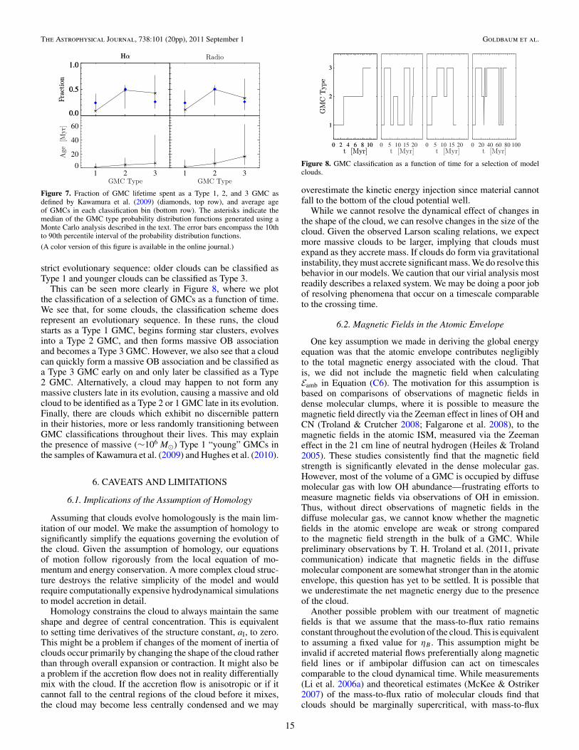
The Astrophysical Journal, 738:101 (20pp), 2011 September 1 Goldbaum et al.
Figure 7. Fraction of GMC lifetime spent as a Type 1, 2, and 3 GMC asdefined by Kawamura et al. (2009) (diamonds, top row), and average ageof GMCs in each classification bin (bottom row). The asterisks indicate themedian of the GMC type probability distribution functions generated using aMonte Carlo analysis described in the text. The error bars encompass the 10thto 90th percentile interval of the probability distribution functions.
(A color version of this figure is available in the online journal.)
strict evolutionary sequence: older clouds can be classified asType 1 and younger clouds can be classified as Type 3.
This can be seen more clearly in Figure 8, where we plotthe classification of a selection of GMCs as a function of time.We see that, for some clouds, the classification scheme doesrepresent an evolutionary sequence. In these runs, the cloudstarts as a Type 1 GMC, begins forming star clusters, evolvesinto a Type 2 GMC, and then forms massive OB associationand becomes a Type 3 GMC. However, we also see that a cloudcan quickly form a massive OB association and be classified asa Type 3 GMC early on and only later be classified as a Type2 GMC. Alternatively, a cloud may happen to not form anymassive clusters late in its evolution, causing a massive and oldcloud to be identified as a Type 2 or 1 GMC late in its evolution.Finally, there are clouds which exhibit no discernible patternin their histories, more or less randomly transitioning betweenGMC classifications throughout their lives. This may explainthe presence of massive (∼106 M�) Type 1 “young” GMCs inthe samples of Kawamura et al. (2009) and Hughes et al. (2010).
6. CAVEATS AND LIMITATIONS
6.1. Implications of the Assumption of Homology
Assuming that clouds evolve homologously is the main lim-itation of our model. We make the assumption of homology tosignificantly simplify the equations governing the evolution ofthe cloud. Given the assumption of homology, our equationsof motion follow rigorously from the local equation of mo-mentum and energy conservation. A more complex cloud struc-ture destroys the relative simplicity of the model and wouldrequire computationally expensive hydrodynamical simulationsto model accretion in detail.
Homology constrains the cloud to always maintain the sameshape and degree of central concentration. This is equivalentto setting time derivatives of the structure constant, aI, to zero.This might be a problem if changes of the moment of inertia ofclouds occur primarily by changing the shape of the cloud ratherthan through overall expansion or contraction. It might also bea problem if the accretion flow does not in reality differentiallymix with the cloud. If the accretion flow is anisotropic or if itcannot fall to the central regions of the cloud before it mixes,the cloud may become less centrally condensed and we may
Figure 8. GMC classification as a function of time for a selection of modelclouds.
overestimate the kinetic energy injection since material cannotfall to the bottom of the cloud potential well.
While we cannot resolve the dynamical effect of changes inthe shape of the cloud, we can resolve changes in the size of thecloud. Given the observed Larson scaling relations, we expectmore massive clouds to be larger, implying that clouds mustexpand as they accrete mass. If clouds do form via gravitationalinstability, they must accrete significant mass. We do resolve thisbehavior in our models. We caution that our virial analysis mostreadily describes a relaxed system. We may be doing a poor jobof resolving phenomena that occur on a timescale comparableto the crossing time.
6.2. Magnetic Fields in the Atomic Envelope
One key assumption we made in deriving the global energyequation was that the atomic envelope contributes negligiblyto the total magnetic energy associated with the cloud. Thatis, we did not include the magnetic field when calculatingEamb in Equation (C6). The motivation for this assumption isbased on comparisons of observations of magnetic fields indense molecular clumps, where it is possible to measure themagnetic field directly via the Zeeman effect in lines of OH andCN (Troland & Crutcher 2008; Falgarone et al. 2008), to themagnetic fields in the atomic ISM, measured via the Zeemaneffect in the 21 cm line of neutral hydrogen (Heiles & Troland2005). These studies consistently find that the magnetic fieldstrength is significantly elevated in the dense molecular gas.However, most of the volume of a GMC is occupied by diffusemolecular gas with low OH abundance—frustrating efforts tomeasure magnetic fields via observations of OH in emission.Thus, without direct observations of magnetic fields in thediffuse molecular gas, we cannot know whether the magneticfields in the atomic envelope are weak or strong comparedto the magnetic field strength in the bulk of a GMC. Whilepreliminary observations by T. H. Troland et al. (2011, privatecommunication) indicate that magnetic fields in the diffusemolecular component are somewhat stronger than in the atomicenvelope, this question has yet to be settled. It is possible thatwe underestimate the net magnetic energy due to the presenceof the cloud.
Another possible problem with our treatment of magneticfields is that we assume that the mass-to-flux ratio remainsconstant throughout the evolution of the cloud. This is equivalentto assuming a fixed value for ηB . This assumption might beinvalid if accreted material flows preferentially along magneticfield lines or if ambipolar diffusion can act on timescalescomparable to the cloud dynamical time. While measurements(Li et al. 2006a) and theoretical estimates (McKee & Ostriker2007) of the mass-to-flux ratio of molecular clouds find thatclouds should be marginally supercritical, with mass-to-flux
15

The Astrophysical Journal, 738:101 (20pp), 2011 September 1 Goldbaum et al.
ratios of order unity, the time evolution and cloud-to-cloudvariation in mass-to-flux ratios are poorly constrained.
6.3. Validity of Larson’s Laws
It has been suggested that the observed constancy of GMCsurface densities is an artifact (see, e.g., Kegel 1989; Vazquez-Semadeni et al. 1997; Murray 2011). Since the physical structurewe assume for the clouds in our model implicitly assumes thatthe Larson relations are valid, this may imply that our modelsdo not correspond well to real GMCs.
The argument that the Larson laws are a product of a selectioneffect usually proceeds as follows. If one looks for overdensitiesof a particular size in a simulation of the turbulent ISM, one willfind that the selected clouds have a wide distribution of masses,implying a large spread in cloud-to-cloud surface density. Sinceobservers detect clouds using CO as a tracer and at low surfacedensity the CO abundance is not high enough to be detectable inemission, observers will never find low surface density clouds.This implies that, at a fixed radius, real clouds should havemore variation in mass than a naive interpretation of the COobservations would suggest.
This argument misses two key aspects of the observedproperties of GMCs. The first is that it cannot explain the lack ofGMCs with high gas surface densities. For the same reason thatwe should not be able to see diffuse clouds, we should very easilybe able to see compact, high surface density CO clouds. The factthat these clouds do not exist implies something important aboutthe structure of GMCs. The second argument is that the lack oflow surface density clouds does not imply that molecular cloudscan exist at all surface densities but merely that the molecularclouds dissociate once they become optically thin to the ambientultraviolet radiation field. While diffuse atomic clouds certainlyexist, these clouds do not form stars (Krumholz et al. 2011).
Since high surface density GMCs are not observed in the lo-cal universe and low surface density clouds are not molecularand thus not GMCs by definition, the observed lack of variationin GMC surface densities must be a real property of the clouds.This has been confirmed with very detailed dust extinction mea-surements of nearby star-forming clouds, where an exquisitelytight mass–radius relation is observed (Lombardi et al. 2010)and in extragalactic studies where little variation is seen whencomparing the mass–radius relation from galaxy to galaxy(Bolatto et al. 2008). Taken together, the evidence seems toimply that the Larson relations are a property of the structure ofGMCs and are not due to a selection effect.
7. CONCLUSIONS
In this paper, we have presented semianalytic dynamicalmodels for the evolution of GMCs undergoing both massaccretion and star formation. These models are able to capturethe evolution of individual GMCs from their growth and theonset of massive star formation, until their dispersal via anenergetic H ii region or through the combined action of accretionand star formation. We are able for the first time to synthesizegalactic populations of GMCs whose properties correspondclosely to the observed properties of GMCs in the Milky Wayand nearby external galaxies. We have shown that clouds inlow surface density environments generally disperse within afew crossing times, before they can accrete all of the gas intheir reservoir. At the same time, clouds in high surface densityenvironments do accrete all of the gas in their reservoirs andtend to be larger and more massive. We have also shown
that mass accretion can contribute a significant fraction ofthe total energy available for turbulent driving. Lastly, wegenerate synthetic cluster observations and compare againstthe evolutionary classification scheme of Kawamura et al.(2009), finding good agreement when we correct for selectioneffects and systematic biases inherent in the observations. Weconclude that, on average, the evolutionary classification schemecorresponds to an age sequence but is not a good predictor forthe evolutionary state of isolated clouds.
We thank Leo Blitz and Adam Leroy for making availablethe Milky Way data used in Figures 5 and 6. We also thank ananonymous referee for their helpful comments which spurreda significant improvement in the quality of the paper. N.J.G. issupported by a Graduate Research Fellowship from the NationalScience Foundation. M.R.K. acknowledges support from anAlfred P. Sloan Fellowship, NSF grants AST-0807739 andCAREER-0955300, and NASA through Astrophysics Theoryand Fundamental Physics grant NNX09AK31G and a SpitzerSpace Telescope Theoretical Research Program grant. C.D.M.’sresearch is supported by an NSERC discovery grant and anOntario Early Researcher Award. The research of C.F.M. issupported in part by NSF grant AST-0908553 and by a SpitzerSpace Telescope Theoretical Research Program grant.
APPENDIX A
DERIVATION OF THE VIRIAL THEOREM FOR ANACCRETING CLOUD
Here, we derive an equation governing the virial balanceof a cloud that is simultaneously forming stars and accretingmaterial. This is a generalization of the analysis of Paper I andMcKee & Zweibel (1992). We refer the reader to those papers fordetails that are unrelated to the accretion flow and to Section 2.1for a general overview of the model.
Consider a single molecular cloud contained within anEulerian volume Vvir with bounding surface Svir. We assumethat Vvir is sufficiently large to contain the cloud at all times.Material within the virial volume is apportioned into threecomponents: virial material, a gaseous reservoir, and material ina photoionized wind. Locally, each component satisfies its owncontinuity equation,
∂ρ
∂t= −∇ · ρv + ρ (A1)
∂ρres
∂t= −∇ · ρresvres − ρacc (A2)
∂ρw
∂t= −∇ · ρwvw − ρej. (A3)
These equations are coupled via the source and sink terms,
ρ = ρacc + ρej. (A4)
We assume that accretion can only transport material onto thecloud and that the wind can only carry material away from thecloud, implying ρacc � 0 and ρej � 0.
The local equation of momentum conservation for the virialmaterial is (cf. Equation (A2) in Paper I)
∂
∂t(ρv) = −∇·(Π−TM)+ρg+F∗+ρej(v+v′
ej)+ρaccvres, (A5)
16

The Astrophysical Journal, 738:101 (20pp), 2011 September 1 Goldbaum et al.
where Π = PthI + ρvv − π is the gas pressure tensor, π isthe viscous stress tensor, TM = [BB − (1/2)B2I]/(4π ) is theMaxwell stress tensor, B is the magnetic field, I is the unit tensor,g is the gravitational force per unit mass, and F∗ + ρej(v + v′
ej) isthe local body force due to the interaction between expandingH ii regions and the cloud. We write the stellar forcing term inthis form so as to separate the random component, F∗, from thespherically symmetric component ρej(v + v′
ej).F∗ is a function of time and position in the cloud and depends
on the precise location and history of massive star formation.Due to the nature of supersonic turbulence, we expect turbulentoverdensities to be randomly scattered throughout the cloud.Thus, we expect F∗ to be randomly oriented with respect tothe position vector, implying
∫Vvir
r · F∗dV = 0. While F∗ israndomly oriented, ρej(v+v′
ej) should on average be purely radialbecause the photoionized wind will be blown out preferentiallyalong the pressure gradient. Neither F∗ nor the viscous stresstensor is included in the momentum equation used in PaperI. A detailed comparison of the two approaches leads us toconclude that the formulation used here more properly followsthe transport of energy through the turbulent cascade.
After taking the second time derivative of the cloud momentof inertia, Icl = ∫
Vvirρr2dV , and substituting the momentum
Equation (A5) into the resulting expression, we find
1
2Icl = 1
2
d
dt
∫Vvir
ρr2dV − 1
2
d
dt
∫Svir
ρvr2 · dS
+∫
Vvir
r · [ρg + F∗ − ∇ · (Π − TM)]dV
+∫
Vvir
ρejr · (v + v′ej)dV +
∫Vvir
ρaccr · vresdV.
(A6)
Upon evaluating the integrals in Equation (A6) term by term,we obtain the EVT,
1
2Icl = 2(T − T0) + B + W
− 1
2
d
dt
∫Svir
(ρvr2) · dS + aIMclRclRcl
+1
2aIMclR
2cl + aIMejRclRcl
+3 − kρ
4 − kρ
Rcl(Mejv′ej − ξMaccvesc). (A7)
Here T , T0, B, and W are, respectively, the standard kinetic,surface kinetic, magnetic, and gravitational terms (see Paper Ifor precise definitions) and aI = (3 − kρ)/(5 − kρ). The finalterm in Equation (A7) does not appear in the EVT derived inPaper I and is due to the presence of the accretion flow. This hasthe same form as the wind recoil term except for the presenceof a dimensionless factor
ξ =∫ 1
0(4 − kρ)x3−kρ
{1 + f
[1 − x2−kρ
2 − kρ
+∫ 1
x
y(x ′)x ′2 dx ′
]}dx
(A8)which arises because material is accreted at a velocity thatdepends on the depth of the cloud potential well. The di-mensionless variables x, y, and f are defined explicitly inAppendix B.
The magnetic term B retains the form used in Paper I andderived by McKee & Zweibel (1992) because we assume any
deformation of the magnetic field in the ambient medium causedby the presence of the cloud is negligible at the virial surface,allowing us to approximate that the virial volume is threadedby a constant magnetic field B0. Here, B0 is the rms value ofthe true magnetic field at the virial surface, which may fluctuatearound B0. Since material in the reservoir should also carrycurrents and thus generate magnetic fields, this parameterizationunderestimates the total magnetic energy. However, we expectthe mean density of reservoir material within the virial volumeto be an order of magnitude smaller than the density of cloudmaterial (see Appendix B), so the contribution of the reservoirto the magnetic energy is small compared to the contributiondue to the cloud.
APPENDIX B
PROPERTIES OF THE RESERVOIR
Consider an accreting cloud that is not forming stars and thusnot generating a wind. Let Mres(r, t) be the mass of materialin the accretion flow contained within a radius r at time t andlet Δr = vres,sysΔt be the distance that the accreting gas fallsin a time Δt . In the same time, a fraction of the material inthe accretion flow will be converted into cloud material. In theframe comoving with the accretion flow, the change in the massof reservoir interior to a radius r in a time Δt is
Mres(r, t) − Mres(r − Δr, t + Δt) = −Δt
∫ r
0ρaccdV. (B1)
Upon Taylor expanding in Δt and Δr , dropping the nonlinearterms, and evaluating the integral on the right-hand side ofEquation (B3), we find
Δr∂Mres(r, t)
∂r− Δt
∂Mres(r, t)
∂t= −Macc(r, t)Δt. (B2)
If the accretion flow is in a quasi-steady state, the time derivativevanishes and Mres(r, t) = Mres(r). Integrating to obtain Mres(r),we find
Mres(r) = −∫ r
0
Macc(r ′)vres,sys(r ′)
dr ′. (B3)
If we wish to evaluate the above integral and obtain anexpression for Mres(r), we need to know vres,sys(r). ExpandingEquation (4), we see
1
2v2
res,sys(r) = −∫ Rcl
∞
G(Mcl + Mres)
r ′2 dr ′
−∫ r
Rcl
GMcl(r ′)r ′2
[(r ′
Rcl
)3−kρ
+Mres(r ′)Mcl(r ′)
]dr ′.
(B4)
Equations (B3) and (B4) constitute a system of integral equa-tions that must be simultaneously solved to obtain a solu-tion for the velocity and mass profile of reservoir materialwithin the cloud volume. If we define the functions x =r/Rcl, y(x) = Mres(Rclx)/Mcl, and f = Mcl/(Mres + Mcl),Equation (B4) reduces to
vres,sys(r) = −vesc
[1 + f
(1 − x2−kρ
2 − kρ
−∫ x
1
y(x ′)x ′2 dx ′
)]1/2
.
(B5)
17

The Astrophysical Journal, 738:101 (20pp), 2011 September 1 Goldbaum et al.
Figure 9. (a) y (dotted line) and z (dashed line) as a function of x = r/Rcl. (b) y(1) = Mres(Rcl)/Mcl as a function of ζ = Macctff/Mcl. We see Mres(Rcl) � Mclfor ζ � 5.
Defining ζ = Macctff/Mcl and z(x) = ∫ 1x
y(x ′)/x ′2dx ′, wesee that the problem of determining both vres,sys(r) and Mres(r)reduces to solving the following system of nonlinear ordinarydifferential equations:
dy
dx= 2
πζx3−kρ
[1 + f
(1 − x2−kρ
2 − kρ
+ z(x)
)]−1/2
, (B6)
dz
dx= −y(x)
x2. (B7)
These equations can be solved numerically using the shootingmethod as follows. Since there should be no unmixed accretedmaterial at r = 0, we expect y(0) = 0. Since z(x) is definedin terms of an integral, we have no a priori knowledge of z(0).However, we do know that z(1) = 0 and we expect y(1) � ζ .If we impose y(1) = c ζ where c is a constant of order unity,we can integrate the above system and obtain a trial solution fory(x) and z(x). The constant c can then be varied until a solutionis obtained with y(0) = 0. There is a unique solution for eachvalue of ζ and thus a new solution must be obtained if ζ varies.
A key assumption in this analysis was that the accretion rate isapproximately constant over the cloud free-fall timescale. Thisis equivalent to the assumption that ζ � 1. This is a reasonableassumption, which we can see by making an analogy to the caseof a protostellar core. Since we expect Mcl ≈ Mcl/tff,r wheretff,r is the free-fall time for all of the gas in the reservoir (Stahleret al. 1980; McKee & Tan 2003) and since the reservoir shouldbe significantly more extended than the cloud, we expect themean density of the reservoir to be much lower than the meandensity in the cloud. This implies tff,r tff,cl. If this conditiondoes hold, then the condition ζ � 1 is automatically satisfied.
In Figure 9(a) we present a numerical solution for y(x)and z(x) obtained for ζ = 1.0. We see for this case thatMres(Rcl) ≈ 0.2Mcl, showing that even for substantial accretionrates, the gas within Vcl is primarily composed of cloud material.In Figure 9(b) we show y(1) = Mres(Rcl)/Mcl as a function of ζ .Reservoir material becomes the primary component of the vol-ume occupied by the cloud for ζ � 5.0. For this reason, we rejectas unphysical any portion of cloud history with ζ � 5. In prac-tice, we find ζ � 1.0 for the lifetime of all clouds we simulate.
APPENDIX C
DERIVATION OF THE EQUATION OF ENERGYCONSERVATION FOR AN ACCRETING CLOUD
Here, we derive the global equation of energy conserva-tion for a cloud undergoing accretion and star formation.
We begin by writing the equation of momentum conservation(Equation (A5)) in Lagrangian form:
ρdvdt
= −∇P −ρ∇φ+∇·π +J × B
c+ρejv′
ej+F∗+ρacc(vres−v).
(C1)Upon contracting the above equation with v, we obtain thenonthermal energy evolution equation,
∂
∂t
(1
2ρv2 + ρφcl +
B2 − B20
8π
)+ ∇ · ρv
(1
2v2 + φcl
)+ ∇ · SP
= −v · ∇P + ρ∂φcl
∂t+ ρv · gres + ∇ · (π · v)
− π : ∇v + ρ
(1
2v2 + φcl
)+ v · F∗ + ρejv · v′
ej
+ ρacc(v · vres − v2), (C2)
where SP is the Poynting vector. Combining the first lawof thermodynamics with the continuity equation yields theevolution equation for the thermal energy of the cloud,
∂
∂t(ρe) + ∇ · ρv
(e +
P
ρ
)= ρe + v · ∇P + Γ − Λ, (C3)
where e is the internal energy per unit mass and Γ and Λare, respectively, the rates of energy gain and loss per unitvolume. Here we have assumed that accreted material hasthe same thermal energy density as cloud material, whichwill be true if the radiative timescales are short compared tothe mechanical timescales, as in molecular cloud conditions.Summing Equations (C2) and (C3), we obtain the evolutionequation for the total energy of the system:
∂
∂t
[ρ
(1
2v2 + e +
1
2φcl
)+
B2 − B20
8π
]
+ ∇ · ρv(
1
2v2 + e +
P
ρ+ φcl
)+ ∇ · SP
= 1
2
(ρ
∂φcl
∂t− ∂ρ
∂tφcl
)+ ρ
(1
2v2 + e +
1
2φcl
)+
1
2ρφcl
+ ρv · gres + ρejv · v′ej + ρacc(v · vres − v2) + ∇ · (π · v)
+ v · F∗ − Λ. (C4)
Here we have assumed that Γ = π :∇v, the scalar rate ofviscous dissipation. This is equivalent to the statement that
18

The Astrophysical Journal, 738:101 (20pp), 2011 September 1 Goldbaum et al.
turbulent kinetic energy is converted into heat at viscous scaleswhereupon the energy is quickly radiated away. While theremay be other heating mechanisms, including cosmic rays andprotostellar radiation, we neglect these sources by noting thatany local heating should be offset in a time much shorter thanthe dynamical time.
If we define the total energy due to the presence of the cloud,
Ecl =∫
Vcl
ρ
(1
2v2 + e +
1
2φcl
)dV +
∫Vvir
B2 − B20
8πdV, (C5)
and the total energy in the ambient medium,
Eamb =∫
Vvir−Vcl
ρ
(1
2v2 + e +
1
2φcl
)dV, (C6)
we can integrate Equation (C4) over the virial volume andobtain an evolution equation for Ecl. Portions of this calculationare performed explicitly in Paper I and we do not reproducethose results here. The new terms stem from our inclusion ofaccretion as well as the inclusion of F∗, the random componentof the stellar forcing term. The integrals over the new terms areevaluated below.
The first new term is due to the gravitational influence of thereservoir, ∫
Vvir
ρv · gresdV = −χRcl
Rcl
GM2cl
Rcl, (C7)
where
χ = (3 − kρ)∫ 1
0x1−kρ y(x)dx. (C8)
This is the gravitational work done on the cloud by the reservoirmaterial as the cloud expands and contracts.
The random stellar forcing term can be evaluated by notingthat r and F∗ are assumed to be uncorrelated, so
∫Vvir
v · F∗dV
= ∫Vvir
vturb · F∗dV . This integral depends on the degree ofcorrelation between two randomly oriented vectors, vturb andF∗. Since, at a fixed time, the direction of expansion of anH ii region is the same as the direction of momentum injection,these vectors should indeed be highly correlated. This term thencorresponds to the net injection of energy by H ii regions,
Gcl =∫
Vvir
vturb · F∗dV. (C9)
For the terms proportional to ρacc, we have∫Vvir
ρaccv · vresdV = −(
3 − kρ
4 − kρ
)ξRclMaccvesc
+∫
Vvir
ρaccvturb · vresdV (C10)
and ∫Vvir
ρaccv2dV = aIMaccR
2cl + 3Maccσ
2cl, (C11)
where we have used our assumption that vres,rand is randomlyoriented with respect to r.
We are left with one last integral on the right-hand side ofEquation (C10) that depends on the correlation between twovector fields, vturb and vres. Suppose vres and vturb are perfectlycorrelated. In that case, the integral we are concerned with can be
readily evaluated in three limits, |vres| = |vturb|, |vres| |vturb|,and |vres| � |vturb|. In the first limit |vres| = |vturb| the transferof material to the cloud is merely an act of relabeling, sovturb · vres = v2
res. Now consider the limit |vres| |vturb|. Weapproximate that a parcel of reservoir material mixes with thecloud once it has swept up a mass of cloud material equalto its own mass. Since the interaction between cloud materialand reservoir material must be inelastic if they are to mix, thevelocity of cloud material must be driven by the act of mixingto vturb = vres/2. Conversely, if |vres| � |vturb|, the reservoirmaterial is driven to a velocity vres = vturb/2. We obtain thecorrect answer in all three limits if we assume∫
Vvir
ρaccvturb · vresdV = 1
2
∫Vvir
ρacc(v2
res + v2turb
)dV. (C12)
This is an upper bound on the value of the integral in the limitof perfect correlation between vturb and vres. If vturb and vres areuncorrelated then the integrand should on average be zero. Thuswe have
0 �∫
Vvir
ρaccvturb · vresdV � 1
2
∫Vvir
ρacc(v2res + v2
turb)dV.
(C13)To evaluate this integral, we linearly interpolate between theupper limit and lower limit,∫
Vvir
ρaccvturb · vresdV = ϕ1
2
∫Vvir
ρacc(v2
res + v2turb
)dV
= ϕ
(3
2Maccσ
2res +
3
2Maccσ
2cl + γ Maccv
2esc
), (C14)
where ϕ is an interpolation parameter that ranges between zeroand unity and
γ = 1
2+ f
(1
10 − 4kρ
− χ
6 − 2kρ
). (C15)
Summing the individual terms derived above yields the globalform of the equation of energy conservation,
dEcl
dt= Mcl
Mcl
[Ecl +
(1 − η2
B
)W
]+
GMclMcl
Rclχ
(1 − MclRcl
MclRcl
)
+
(3 − kρ
4 − kρ
)Rcl(Mejv
′ej − ξMaccvesc)
− 4πPambR2clRcl − aIMaccR
2cl − 3Maccσ
2cl
+ ϕ
(3
2Maccσ
2res +
3
2Maccσ
2cl + γ Maccv
2esc
)+ Gcl − Lcl,
(C16)
where Lcl = ∫Vvir
ΛdV .
REFERENCES
Abel, T., Bryan, G. L., & Norman, M. L. 2002, Science, 295, 93Abdo, A. A., Ackerman, M., Ajello, M., et al. 2010, ApJ, 710, 133Alves, D. R. 2004, New Astron. Rev., 48, 659Ballesteros-Paredes, J. 2006, MNRAS, 372, 443Ballesteros-Paredes, J., Hartmann, L., & Vazquez-Semadeni, E. 1999, ApJ, 527,
285Ballesteros-Paredes, J., Hartmann, L. W., Vazquez-Semadeni, E., Heitsch, F.,
& Zamora-Aviles, M. A. 2011, MNRAS, 411, 65Ballesteros-Paredes, J., & Mac Low, M.-M. 2002, ApJ, 570, 734
19

The Astrophysical Journal, 738:101 (20pp), 2011 September 1 Goldbaum et al.
Bertoldi, F., & McKee, C. F. 1992, ApJ, 395, 140Bica, E., Claria, J. J., Dottori, H., Santos, J. F. C., Jr., & Piatti, A. E. 1996, ApJS,
102, 57Bigiel, F., Leroy, A., Walter, F., et al. 2008, AJ, 136, 2846Blitz, L., Fukui, Y., Kawamura, A., et al. 2007, in Protostars and Planets V, ed.
B. Reipurth, D. Jewitt, & K. Keil (Tucson, AZ: Univ. Arizona Press), 81Blitz, L., & Shu, F. H. 1980, ApJ, 238, 148Bolatto, A. D., Leroy, A. K., Rosolowsky, E., Walter, F., & Blitz, L. 2008, ApJ,
686, 948Brunt, C. M., Heyer, M. H., & Mac Low, M.-M. 2009, A&A, 504, 883Condon, J. J. 1992, ARA&A, 30, 575Dickel, J. R., McIntyre, V. J., Gruendl, R. A., & Milne, D. K. 2005, AJ, 129,
790Dobbs, C. L., Burkert, A., & Pringle, J. E. 2011, MNRAS, 413, 2935Elmegreen, B. G., & Scalo, J. 2004, ARA&A, 42, 211Engargiola, G., Plambeck, R. L., Rosolowsky, E., & Blitz, L. 2003, ApJS, 149,
343Evans, N. J., Dunham, M. M., Jørgensen, J. K., et al. 2009, ApJS, 181, 321Falgarone, E., Troland, T. H., Crutcher, R. M., & Paubert, G. 2008, A&A, 487,
247Fall, S. M., Krumholz, M. R., & Matzner, C. D. 2010, ApJ, 710, L142Fukui, Y., & Kawamura, A. 2010, ARA&A, 48, 547Fukui, Y., Kawamura, A., Wong, T., et al. 2008, ApJS, 178, 56Glover, S. C. O., Federrath, C., Mac Low, M.-M., & Klessen, R. S. 2010,
MNRAS, 404, 2Goldreich, P., & Kwan, J. 1974, ApJ, 189, 441Heiles, C., & Troland, T. H. 2005, ApJ, 624, 773Heyer, M. H., & Brunt, C. M. 2004, ApJ, 615, L45Heyer, M. H., Carpenter, J. M., & Snell, R. L. 2001, ApJ, 551, 852Heyer, M., Krawczyk, C., Duval, J., & Jackson, J. M. 2009, ApJ, 699, 1092Hughes, A., Staveley-Smith, L., Kim, S., Wolleben, M., & Filipovic, M.
2007, MNRAS, 382, 543Hughes, A., Wong, T., Ott, J., et al. 2010, MNRAS, 406, 2065Hunter, C. 1977, ApJ, 218, 834Imara, N., Bigiel, F., & Blitz, L. 2011, ApJ, 732, 79Kalberla, P. M. W., & Dedes, L. 2008, A&A, 487, 951Kawamura, A., Mizuno, Y., Minamidani, T., et al. 2009, ApJS, 184, 1Kegel, W. H. 1989, A&A, 225, 517Kennicutt, R. C., Jr., Calzetti, D., Water, F., et al. 2007, ApJ, 671, 333Kennicutt, R. C., Jr., & Hodge, P. W. 1986, ApJ, 306, 130Kim, W.-T., & Ostriker, E. C. 2006, ApJ, 646, 213Kim, W.-T., Ostriker, E. C., & Stone, J. M. 2002, ApJ, 581, 1080Kim, W.-T., Ostriker, E. C., & Stone, J. M. 2003, ApJ, 599, 1157Klessen, R. S., & Hennebelle, P. 2010, A&A, 520, A17Kroupa, P. 2002, Science, 295, 82Krumholz, M. R., Leroy, A. K., & McKee, C. F. 2011, ApJ, 731, 25Krumholz, M. R., & Matzner, C. D. 2009, ApJ, 703, 1352Krumholz, M. R., Matzner, C. D., & McKee, C. F. 2006, ApJ, 653, 361Krumholz, M. R., & McKee, C. F. 2005, ApJ, 630, 250Krumholz, M. R., McKee, C. F., & Tumlinson, J. 2008, ApJ, 689, 865Krumholz, M. R., & Tan, J. C. 2007, ApJ, 654, 304Lada, C. J., Lombardi, M., & Alves, J. F. 2010, ApJ, 724, 687Larson, R. B. 1981, MNRAS, 194, 809Lejeune, T., & Schaerer, D. 2001, A&A, 366, 538Leroy, A., Bolatto, A., Stanimirovic, S., et al. 2007, ApJ, 658, 1027Leroy, A. K., Walter, F., Brinks, E., et al. 2008, AJ, 136, 2782Li, H., Griffin, G. S., Krejny, M., et al. 2006a, ApJ, 648, 340Li, Y., Mac Low, M.-M., & Klessen, R. S. 2006b, ApJ, 639, 879Li, Z.-Y., & Nakamura, F. 2006, ApJ, 640, L187Li, Z.-Y., Wang, P., Abel, T., & Nakamura, F. 2010, ApJ, 720, L26Lombardi, M., Alves, J., & Lada, C. J. 2010, A&A, 519, L7Lopez, L. A., Krumholz, M. R., Bolatto, A. D., Prochaska, J. X., & Ramirez-
Ruiz, E. 2011, ApJ, 731, 91Mac Low, M.-M., & Klessen, R. S. 2004, Rev. Mod. Phys., 76, 125
Mac Low, M.-M., Klessen, R. S., Burkert, A., & Smith, M. D. 1998, Phys. Rev.Lett., 80, 2754
Matzner, C. D. 2001, in ASP Conf. Proc. 243, From Darkness to Light: Originand Evolution of Young Stellar Clusters, ed. T. Montmerle & P. Andre (SanFrancisco, CA: ASP), 757
Matzner, C. D. 2002, ApJ, 566, 302Matzner, C. D., & McKee, C. F. 2000, ApJ, 545, 364McKee, C. F. 1989, ApJ, 345, 782McKee, C. F. 1999, in NATO ASIC Proc. 540, The Origin of Stars and Planetary
Systems, ed. C. J. Lada & N. D. Kylafis (Dordrecht: Kluwer), 29McKee, C. F., & Ostriker, E. C. 2007, ARA&A, 45, 565McKee, C. F., & Tan, J. C. 2003, ApJ, 585, 850McKee, C. F., & Williams, J. P. 1997, ApJ, 476, 144McKee, C. F., & Zweibel, E. G. 1992, ApJ, 399, 551Meynet, G., Maeder, A., Schaller, G., Schaerer, D., & Charbonnel, C. 1994,
A&AS, 103, 97Mizuno, N., Rubio, M., Mizuno, A., et al. 2001, PASJ, 53, L45Murray, N. 2011, ApJ, 729, 133Norman, C., & Silk, J. 1980, ApJ, 238, 158Onodera, S., Kuno, N., Tosaki, T., et al. 2010, ApJ, 722, L127Ossenkopf, V., & Mac Low, M.-M. 2002, A&A, 390, 307Parravano, A., Hollenbach, D. J., & McKee, C. F. 2003, ApJ, 584, 797Roman-Duval, J., Jackson, J. M., Heyer, M., Rathborne, J., & Simon, R.
2010, ApJ, 723, 492Rosolowsky, E. 2005, PASP, 117, 1403Rosolowsky, E. 2007, ApJ, 654, 240Rosolowsky, E., & Leroy, A. 2006, PASP, 118, 590Schaerer, D., Meynet, G., Maeder, A., & Schaller, G. 1993, A&AS, 98,
523Schlegel, D. J., Finkbeiner, D. P., & Davis, M. 1998, ApJ, 500, 525Schruba, A., Leroy, A. K., Walter, F., Sandstrom, K., & Rosolowsky, E.
2010, ApJ, 722, 1699Schruba, A., Leroy, A. K., Walter, F., et al. 2011, AJ, 142, 37Shu, F. H. 1977, ApJ, 214, 488Solomon, P. M., Rivolo, A. R., Barrett, J., & Yahil, A. 1987, ApJ, 319, 730Stahler, S. W., Shu, F. H., & Taam, R. E. 1980, ApJ, 241, 637Stark, A. A., & Lee, Y. 2006, ApJ, 641, L113Stone, J. M., Ostriker, E. C., & Gammie, C. F. 1998, ApJ, 508, L99Strong, A. W., & Mattox, J. R. 1996, A&A, 308, L21Tamburro, D., Rix, H.-W., Walter, F., et al. 2008, AJ, 136, 2872Tan, J. C., & McKee, C. F. 2004, ApJ, 603, 383Tan, J. C., Krumholz, M. R., & McKee, C. F. 2006, ApJ, 641, L121Tasker, E. J. 2011, ApJ, 730, 11Tasker, E. J., & Tan, J. C. 2009, ApJ, 700, 358Thilker, D. A., Braun, R., & Walterbos, R. A. M. 2002, in ASP Conf. Ser. 276,
Seeing Through the Dust: The Detection of H i and the Exploration of theISM in Galaxies, ed. A. R. Taylor, T. L. Landecher, & A. G. Willis (SanFrancisco, CA: ASP), 370
Troland, T. H., & Crutcher, R. M. 2008, ApJ, 680, 457van Dishoeck, E. F., & Black, J. H. 1988, ApJ, 334, 771Vazquez-Semadeni, E., Ballesteros-Paredes, J., & Rodriguez, L. F. 1997, ApJ,
474, 292Vazquez-Semadeni, E., Colın, P., Gomez, G. C., Ballesteros-Paredes, J., &
Watson, A. W. 2010, ApJ, 715, 1302Wang, P., & Abel, T. 2008, ApJ, 672, 752Wang, P., Li, Z.-Y., Abel, T., & Nakamura, F. 2010, ApJ, 709, 27Williams, J. P., & McKee, C. F. 1997, ApJ, 476, 166Wise, J. H., & Abel, T. 2007, ApJ, 665, 899Wolfire, M. G., Hollenbach, D., & McKee, C. F. 2010, ApJ, 716, 1191Wong, T., & Blitz, L. 2002, ApJ, 569, 157Wong, T., et al. 2009, ApJ, 696, 370Yang, C.-C., Gruendl, R. A., Chu, Y.-H., Mac Low, M.-M., & Fukui, Y.
2007, ApJ, 671, 374Zuckerman, B., & Evans, N. J., II 1974, ApJ, 192, L149
20