Draft version April 2, 2019Typeset using LATEX default style in AASTeX62

High-Resolution Observations of the Molecular Clouds Associated with the Huge H II Region CTB 102

Brandon Marshall,1 Sung-ju Kang,2 C. R. Kerton,1 Youngsik Kim,2, 3 Minho Choi,2 and Miju Kang2

1Iowa State University

Dept. of Physics & Astronomy, 2323 Osborne Dr.

Ames, IA 50011-3160, USA2Korea Astronomy and Space Science Institute

776, Daedeokdae-ro, Yuseong-gu

Daejeon, 34055, Republic of Korea3Daejeon Observatory

213-48, Gwahak-ro, Yuseong-gu, Daejeon, 34128, Republic of Korea

(Received; Revised; Accepted)

Submitted to ApJ

ABSTRACT

We report the first high-resolution (sub-arcminute) large-scale mapping 12CO and 13CO observations

of the molecular clouds associated with the giant outer Galaxy H II region CTB 102 (KR 1). These

observations were made using a newly commissioned receiver system on the 13.7-m radio telescope

at the Taeduk Radio Astronomy Observatory. Our observations show that the molecular clouds have

a spatial extent of 60 × 35 pc and a total mass of 104.8 − 105.0 M�. Infrared data from WISE and

2MASS were used to identify and classify the YSO population associated with ongoing star formation

activity within the molecular clouds. We directly detect 18 class I/class II YSOs and six transition disk

objects. Moving away from the H II region, there is an age/class gradient consistent with sequential

star formation. The infrared and molecular-line data were combined to estimate the star formation

efficiency (SFE) of the entire cloud as well as the SFE for various sub-regions of the cloud. We find

that the overall SFE is between ∼ 5 – 10%, consistent with previous observations of giant molecular

clouds. One of the sub-regions, region 1a, is a clear outlier, with a SFE of 17 – 35% on a 5 pc spatial

scale. This high SFE is more typical for much smaller (sub-pc scale) star-forming cores, and we think

region 1a is likely an embedded massive protocluster.

Keywords: ISM: clouds — ISM: individual objects (CTB 102) — stars: pre-main sequence — HII

regions

1. INTRODUCTION

In this paper we present the first 12CO and 13CO high-resolution (sub-arcminute) large-scale mapping observations

of the molecular clouds associated with the CTB 102 H II region. These observations provide basic data about the

clouds, such as their sizes and masses, and are combined with archival infrared data to explore ongoing star formation

activity associated with the region.

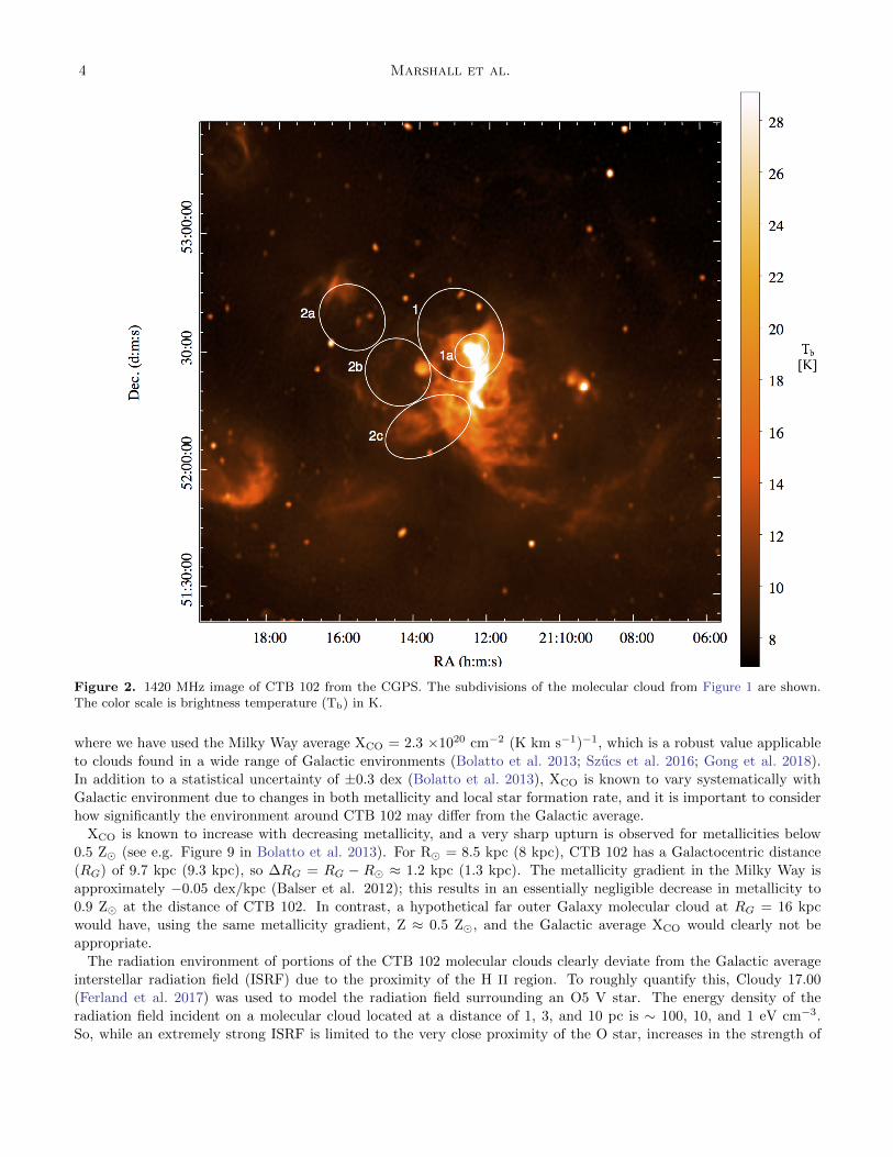
CTB 102 is an enormous H II region/bubble, with an estimated size of 100 – 130 pc, located in the outer Galaxy

(J2000: 21h12m21s, +52◦28′59′′) at a distance d = 4.3 kpc (Arvidsson et al. 2009). It was first identified in low-

resolution radio continuum surveys at 960 and 1420 MHz by Wilson & Bolton (1960) and Kallas & Reich (1980)

respectively, and was imaged with ∼ 1′ resolution at 1420 MHz as part of the Canadian Galactic Plane Survey (CGPS

Taylor et al. 2003). Arvidsson et al. (2009) used H89α radio recombination line observations to show that the extensive

radio continuum structure visible in these surveys was all part of a single object with the primary structure having

Corresponding author: Sung-ju Kang

sjkang@kasi.re.kr

arX

iv:1

904.

0052

9v1

[as

tro-

ph.G

A]

1 A

pr 2

019

2 Marshall et al.

V0,LSR = −62.66 ± 0.05 km s−1 and most of the surrounding filaments having |V − V0| . 6 km s−1. They also

determined that the total Lyman continuum photon emission rate from the region was NLy ≥ (4.5± 1.8)× 1049 s−1,

consistent with a single early-type O star or with a cluster of several late-type O stars.

In spite of its size, CTB 102 has not been studied at optical wavelengths because of both its distance and the fact it

is hidden behind an extensive local region of high extinction (Lynds 1962; Fitzgerald 1968; Simonson & van Someren

Greve 1976). At near- and mid-infrared wavelengths our best view of the region comes from the Wide-field Infrared

Survey Explorer (WISE ; Wright et al. 2010) all-sky survey. A portion of the region was also observed by Spitzer

during its GLIMPSE360 warm-mission survey (Whitney et al. 2008). Comparable resolution data for molecular gas

emission, which is essential for understanding star-formation activity associated with the H II region, was not obtained

until this study.

In section 2 we detail the new 12CO and 13CO observations as well as the archival data that has been collected for

our study. In section 3 the physical properties of the newly mapped molecular clouds are described, and the young

stellar object (YSO) content of the clouds is determined using infrared data. The two studies then are combined to

investigate the star-formation efficiency of the region. Finally, we discuss our findings and present our conclusions in

section 4 and section 5.

2. OBSERVATIONS

2.1. 12CO and 13CO Observations

The CTB 102 H II region was observed using the Second Quabbin Optical Imaging Array in Taeduck Radio Astron-

omy Observatory (SEQUOIA-TRAO) receiver system on the TRAO 13.7-m radio telescope. The data were obtained

between November 2016 and March 2017, during the first observing season after the SEQUOIA receiver array was

relocated from the Five College Radio Astronomy Observatory (FCRAO) and adjusted to the TRAO system. Our

data represent not just the first look at the CTB 102 region at 12CO and 13CO, but also some of the first data obtained

by the SEQUOIA-TRAO system.

We observed 12CO (115.271 GHz, J = 1 − 0) and 13CO (110.201 GHz, J = 1 − 0) lines simultaneously using an

On-The-Fly (OTF) observation mode in a 1.◦5 × 1.◦5 region in order to map the distribution of the molecular gas.

Since the TRAO is a two local oscillator (LO) system, the spectral window has 4096×2 channels in each 62.5 MHz

bandwidth. In total, we observed 36 maps, each a 30′ × 30′ grid, centered on l = 93.◦01, b = 2.◦73. The RMS is

∼ 0.3 K, with a velocity resolution of 0.2 km s−1. This compares favorably with the velocity resolution and RMS of

the Outer Galaxy Survey (OGS; Heyer et al. 1998) and the Galactic Ring Survey (GRS; Jackson et al. 2006) both

obtained at FCRAO: 0.98 km s−1 and 0.65 km s−1 respectively, each with RMS ∼ 0.5 K.

The observed data was reduced using Otftool and the GILDAS software package Class. The pointing of the

observation was calibrated using the SiO ν = 1, J = 2 − 1 maser line in the Orion IRc2 (Baudry et al. 1995). The

pointing observation was performed every two hours, with an average pointing error of ∼ 6′′. The antenna temperature

was corrected automatically for the effects of atmospheric attenuation with a standard chopper-wheel method.

The new radome of TRAO was installed in January 2017 to shield the antenna and receiver from the weather and

other exterior environmental factors. Since the new radome affects the beam efficiency (ηmb), we applied two different

beam efficiencies at 115 GHz, for data acquired before (ηmb = 0.51) and after (ηmb = 0.46) the new radome installation.

The full width at half maximum (FWHM) of the beam at 115 GHz (12CO) is 45′′ and at 110 GHz (13CO) is 48′′.

The integrated 12CO cube is shown in Figure 1, with 13CO contours overlain. For reference, the location of the

molecular clouds are also indicated on the CGPS 1420 MHz image of the region shown in Figure 2.

2.2. Archival Infrared Data

WISE scanned the entire sky in four bands centered at 3.4, 4.6, 12, and 22 µm with a 5σ sensitivity of roughly

16.6, 15.6, 11.3, and 8.0 magnitudes respectively (Wright et al. 2010). We used the Infrared Science Archive (IRSA)

to retrieved all of the sources in the WISE-based AllWISE catalog within a 29 arcminute radius around the center of

the CTB 102 region at l = 93.◦06, b = 2.◦81. No additional constraints were used in the search and we retrieved 14814

sources. The AllWISE catalog also provides the nearest coincident source (≤ 3′′) from the Two Micron All Sky Survey

(2MASS; Skrutskie et al. 2006) All-Sky data release. This provides data in the J, H, and KS bands with magnitude

limits at approximately 16.0, 15.0, and 14.5 magnitudes respectively (Skrutskie et al. 2006).

3. ANALYSIS

The Molecular Clouds of CTB 102 3

Figure 1. Integrated 12CO map of CTB 102. Integration was between VLSR = −71 km s−1 to −53 km s−1. White ellipsesdenote the four main subdivisions of the molecular cloud (1, 2a, 2b, and 2c) along with the smaller 1a region that has a highconcentration of YSOs. Cyan contours show the integrated 13CO emission. Five contour levels were generated starting 3σ abovethe median background. The morphology of the molecular cloud is very similar in both the 12CO and 13CO maps.

3.1. The CTB 102 Molecular Clouds

We adopt the distance to CTB 102 of 4.3 kpc from Arvidsson et al. (2009). This is essentially a kinematic-based

distance that accounts for known non-circular motions in the second quadrant of the Galaxy (Brand & Blitz 1993).

Assuming this, we estimate the overall size of the molecular cloud associated with the region to be approximately

60× 35 pc. Figure 1 shows the 12CO emission integrated over −71 km s−1 < VLSR < −53 km s−1, and indicates the

extent of four distinct subdivisions of the molecular cloud, which were identified from visual inspection of the data

cube. The semi-major and semi-minor axes of region 1 measure approximately 14 × 8 pc, 2a: 9 × 6 pc, 2b: 10 × 9

pc, and 2c: 11× 8 pc (for more precise numbers see Table 1). We also distinguish the region 1a (5× 5 pc), contained

entirely within region 1, due to the high concentration of YSO candidates located within this portion of region 1 (see

Figure 4). Finally, we define a region 2 (28× 16 pc) encompassing regions 2a, 2b, and 2c.

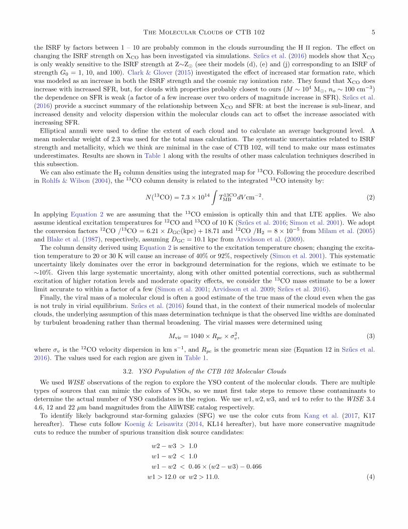
The mass of the molecular clouds associated with CTB 102 can be measured by using the XCO factor to convert

the integrated 12CO intensity into an H2 column density, then integrating the column density over the cloud area.

Column density was calculated using

N(H2) = 2.3× 1020∫T 12COMB dV cm−2, (1)

4 Marshall et al.

Figure 2. 1420 MHz image of CTB 102 from the CGPS. The subdivisions of the molecular cloud from Figure 1 are shown.The color scale is brightness temperature (Tb) in K.

where we have used the Milky Way average XCO = 2.3 ×1020 cm−2 (K km s−1)−1, which is a robust value applicable

to clouds found in a wide range of Galactic environments (Bolatto et al. 2013; Szucs et al. 2016; Gong et al. 2018).

In addition to a statistical uncertainty of ±0.3 dex (Bolatto et al. 2013), XCO is known to vary systematically with

Galactic environment due to changes in both metallicity and local star formation rate, and it is important to consider

how significantly the environment around CTB 102 may differ from the Galactic average.

XCO is known to increase with decreasing metallicity, and a very sharp upturn is observed for metallicities below

0.5 Z� (see e.g. Figure 9 in Bolatto et al. 2013). For R� = 8.5 kpc (8 kpc), CTB 102 has a Galactocentric distance

(RG) of 9.7 kpc (9.3 kpc), so ∆RG = RG − R� ≈ 1.2 kpc (1.3 kpc). The metallicity gradient in the Milky Way is

approximately −0.05 dex/kpc (Balser et al. 2012); this results in an essentially negligible decrease in metallicity to

0.9 Z� at the distance of CTB 102. In contrast, a hypothetical far outer Galaxy molecular cloud at RG = 16 kpc

would have, using the same metallicity gradient, Z ≈ 0.5 Z�, and the Galactic average XCO would clearly not be

appropriate.

The radiation environment of portions of the CTB 102 molecular clouds clearly deviate from the Galactic average

interstellar radiation field (ISRF) due to the proximity of the H II region. To roughly quantify this, Cloudy 17.00

(Ferland et al. 2017) was used to model the radiation field surrounding an O5 V star. The energy density of the

radiation field incident on a molecular cloud located at a distance of 1, 3, and 10 pc is ∼ 100, 10, and 1 eV cm−3.

So, while an extremely strong ISRF is limited to the very close proximity of the O star, increases in the strength of

The Molecular Clouds of CTB 102 5

the ISRF by factors between 1 – 10 are probably common in the clouds surrounding the H II region. The effect on

changing the ISRF strength on XCO has been investigated via simulations. Szucs et al. (2016) models show that XCO

is only weakly sensitive to the ISRF strength at Z∼Z� (see their models (d), (e) and (j) corresponding to an ISRF of

strength G0 = 1, 10, and 100). Clark & Glover (2015) investigated the effect of increased star formation rate, which

was modeled as an increase in both the ISRF strength and the cosmic ray ionization rate. They found that XCO does

increase with increased SFR, but, for clouds with properties probably closest to ours (M ∼ 104 M�, no ∼ 100 cm−3)

the dependence on SFR is weak (a factor of a few increase over two orders of magnitude increase in SFR). Szucs et al.

(2016) provide a succinct summary of the relationship between XCO and SFR: at best the increase is sub-linear, and

increased density and velocity dispersion within the molecular clouds can act to offset the increase associated with

increasing SFR.

Elliptical annuli were used to define the extent of each cloud and to calculate an average background level. A

mean molecular weight of 2.3 was used for the total mass calculation. The systematic uncertainties related to ISRF

strength and metallicity, which we think are minimal in the case of CTB 102, will tend to make our mass estimates

underestimates. Results are shown in Table 1 along with the results of other mass calculation techniques described in

this subsection.

We can also estimate the H2 column densities using the integrated map for 13CO. Following the procedure described

in Rohlfs & Wilson (2004), the 13CO column density is related to the integrated 13CO intensity by:

N(13CO) = 7.3× 1014∫T 13COMB dV cm−2. (2)

In applying Equation 2 we are assuming that the 13CO emission is optically thin and that LTE applies. We also

assume identical excitation temperatures for 12CO and 13CO of 10 K (Szucs et al. 2016; Simon et al. 2001). We adopt

the conversion factors 12CO /13CO = 6.21 ×DGC(kpc) + 18.71 and 12CO /H2 = 8 × 10−5 from Milam et al. (2005)

and Blake et al. (1987), respectively, assuming DGC = 10.1 kpc from Arvidsson et al. (2009).

The column density derived using Equation 2 is sensitive to the excitation temperature chosen; changing the excita-

tion temperature to 20 or 30 K will cause an increase of 40% or 92%, respectively (Simon et al. 2001). This systematic

uncertainty likely dominates over the error in background determination for the regions, which we estimate to be

∼10%. Given this large systematic uncertainty, along with other omitted potential corrections, such as subthermal

excitation of higher rotation levels and moderate opacity effects, we consider the 13CO mass estimate to be a lower

limit accurate to within a factor of a few (Simon et al. 2001; Arvidsson et al. 2009; Szucs et al. 2016).

Finally, the viral mass of a molecular cloud is often a good estimate of the true mass of the cloud even when the gas

is not truly in virial equilibrium. Szucs et al. (2016) found that, in the context of their numerical models of molecular

clouds, the underlying assumption of this mass determination technique is that the observed line widths are dominated

by turbulent broadening rather than thermal broadening. The virial masses were determined using

Mvir = 1040×Rpc × σ2v , (3)

where σv is the 12CO velocity dispersion in km s−1, and Rpc is the geometric mean size (Equation 12 in Szucs et al.

2016). The values used for each region are given in Table 1.

3.2. YSO Population of the CTB 102 Molecular Clouds

We used WISE observations of the region to explore the YSO content of the molecular clouds. There are multiple

types of sources that can mimic the colors of YSOs, so we must first take steps to remove these contaminants to

determine the actual number of YSO candidates in the region. We use w1, w2, w3, and w4 to refer to the WISE 3.4

4.6, 12 and 22 µm band magnitudes from the AllWISE catalog respectively.

To identify likely background star-forming galaxies (SFG) we use the color cuts from Kang et al. (2017, K17

hereafter). These cuts follow Koenig & Leisawitz (2014, KL14 hereafter), but have more conservative magnitude

cuts to reduce the number of spurious transition disk source candidates:

w2− w3 > 1.0

w1− w2 < 1.0

w1− w2 < 0.46× (w2− w3)− 0.466

w1 > 12.0 or w2 > 11.0. (4)

6 Marshall et al.

Table 1. Properties of the CTB 102 molecular clouds

Region 1 1a 2 2a 2b 2c Total

Size (pc)a 14.3 × 8.8 5.2 × 5.0 28.1 × 13.9 8.5 × 5.7 10 × 8.9 11.3 × 8.0 30 × 17.5

Rpcb 11.3 5.1 19.8 7.1 9.4 9.5 · · ·

12CO Avg. V LSR (km s−1) −62.56 −63.21 −62.55 −63.29 −62.34 −62.10 −62.61

σv (km s−1) 1.72 1.44 1.53 1.56 1.31 1.60 1.85

Mass (log M�) 4.27 3.81 4.62 4.00 4.06 4.14 4.7813CO Avg. V LSR (km s−1) −64.46 −64.47 −64.45 −64.44 −64.13 −64.19 −64.57

σv (km s−1) 1.20 1.16 1.23 1.03 1.29 1.15 1.22

Mass (log M�) 3.28 2.64 3.99 3.52 3.56 3.61 4.07

Virial Mass (log M�) 4.54 4.04 4.68 4.26 4.22 4.40 4.95c

aSemi-major and semi-minor axes of the elliptical apertures used to determine the mass of the region from theintegrated 12CO and 13CO data cubes

bGeometric mean size used in the virial mass calculation

cMass determined from the sum of regions 1 and 2

Active galactic nuclei (AGN) with unresolved broad-line regions are another source of false YSOs as their mid-

infrared colors are very similar. These AGN however are expected to be fainter than a typical YSO closer than ∼5

kpc. The criteria used to identify and remove these likely AGNs is again identical to K17:

w1>1.8× (w1− w3) + 4.1

w1>13.0 or w2 > 12.0

or

w1>w1− w3 + 11.0. (5)

After the elimination of the red extragalactic contaminants, there are two sources of galactic contaminants that we

consider. We once again follow the method from K17 to determine whether any of the objects are unresolved shock

emission knots or resolved PAH emission. For shock emission we follow the criteria:

w1− w2> 1.0

w2− w3< 2.0, (6)

and for PAH emission we use:

w1− w2<1.0

w2− w3>4.9

or

w1− w2<0.25

w2− w3>4.75. (7)

Figure 3 illustrates the contaminant identification procedure. Starting with the 14814 sources selected from the

AllWISE catalog, 13223 sources are identified as contaminants, and the remaining 1591 sources move on to the YSO

candidate classification process described in subsubsection 3.2.1.

3.2.1. YSO Classification

After removing all of the likely contaminants, we are ideally left with just field stars and YSO candidates. To identify

and classify YSO candidates we followed the KL14 procedure. For convenience we show the YSO classification scheme

The Molecular Clouds of CTB 102 7

Figure 3. WISE color-color diagram for WISE 3.4, 4.6, and 12 µm bands showing the different contamination cuts describedin subsection 3.2. All 14814 sources extracted from the AllWISE catalog using a spatial search around CTB 102 are plotted.Sources categorized as shock objects, star forming galaxies and PAH emission are found within the boundaries of the black lineson the plot. Source color refers to the WISE 4.6 µm band magnitude.

below, and refer the reader to KL14 for details on how the color cuts were developed. Class I objects, essentially YSOs

with significant infalling envelopes of material, are defined by:

w2− w3>2.0

w1− w2>−0.42× (w2− w3) + 2.2

w1− w2>−0.46× (w2− w3)− 0.9

w2− w3<4.5. (8)

Class II objects, corresponding to YSOs with a significant amount of material in a circumstellar disk, are defined

by:

w1− w2>0.25

w1− w2<0.9× (w2− w3)− 0.25

w1− w2>−1.5× (w2− w3) + 2.1

w1− w2>0.46× (w2− w3)− 0.9

w2− w3<4.5. (9)

Transition disk objects, which perhaps are a more evolved Class II object, are defined by:

w3− w4 > 1.5

0.15 < w1− w2 < 0.8

8 Marshall et al.

Figure 4. RGB image of CTB102 in WISE 24, 12, and 4.6 µm. Red circles correspond to class I sources, magenta diamondsto class II, and cyan boxes to transition disks. Source type comes from the K17 classification given in Table 2. Also shown, aswhite ellipses, are the molecular cloud regions identified in Figure 1.

w1− w2 > 0.46× (w2− w3)− 0.9

w1 ≤ 13.0. (10)

As most of the sources have corresponding 2MASS counterparts, KL14 also developed techniques to identify Class

I and Class II objects using 2MASS and WISE data for sources not classified using only WISE photometry. 2MASS

Class I objects are defined by:

H −KS > −1.76× (w1− w2) + 2.55. (11)

2MASS Class II YSOs are defined by:

H −KS>0.0

H −KS>−1.76× (w1− w2) + 0.9

H −KS< (0.55/0.16)× (w1− w2)− 0.85

w1≤13.0. (12)

We are left with the choice whether or not to consider the χ2 and signal-to-noise cuts from KL14, which are designed

to minimize the number of fake sources that could be potentially classified as YSO candidates. The cuts are the

following:

WISE band 1 (3.4 µm): non-null value for w1sigmpro and w1chi2 < (w1snr − 3)/7,

WISE band 2 (4.6 µm): non-null w2sigmpro,

The Molecular Clouds of CTB 102 9

WISE band 3 (12 µm): w3snr ≥ 5 and either w3chi2 < (w3snr − 8)/8 or 0.45 < w3chi2 < 1.15,

WISE band 4 (22 µm): non-null w4sigmpro and w4chi2 < (2× w4snr − 20)/10,

where snr, chi2, and sigmpro are the source signal-to-noise, χ2, and photometric uncertainty respectively.

Each band cut is applied to the source as that band is required for the classification. For example, only transition

disk objects must pass the WISE band 4 cut, as these are the only object that require w4 to be classified as such.

When following the exact KL14 technique we are left with 18 YSOs. However a visual inspection of the region shows

that 11 of those sources do not appear to be reliable, leaving us with 7 YSO candidates using the KL14 method.

However if we follow the approach used by K17, we can disregard the χ2 and signal-to-noise cuts and use a visual

inspection to identify spurious YSO candidates after the initial classifications are made. Using this procedure we

initially found 128 YSO candidates. The subsequent visual inspection removed 104 sources leaving a total of 24 YSOs

(see Figure 5).

The quality checks from KL14 are very effective at removing spurious sources, and are best used when investigating

very large spatial regions. For a smaller area, such as in this study, visual inspection and removal of spurious sources

is still practical and results in a better picture of the YSO population. We find 18 Class I and II YSO candidates

using this technique, 11 more than from using the KL14 technique. We also find 6 transition disk objects, whereas

KL14 identifies none. A number of the transition disk YSOs appear around a 24 µm bubble-like structure as seen in

Figure 4; however, due to the uncertainty in the evolutionary stage of transition disks, the focus the rest of our study

will be on the 18 Class I and Class II YSO candidates (our ‘best candidate’ sample). The YSO classifications for this

sample based on WISE and 2MASS colors are shown in column 2 of Table 2. Photometry and source designations for

this sample and the 6 transition disk candidates are listed in Table 4 and Table 5 in the Appendix.

3.2.2. Classification via SED Modeling

We also classify the YSO candidates in our ‘best candidate’ sample using a slightly modified version of the technique

described by Alexander et al. (2013). This technique uses the Robitaille et al. (2007) spectral energy distribution

(SED) fitting tool to match candidate YSO SEDs to the suite of YSO models from Robitaille et al. (2006). Initially,

we attempt to fit reddened stellar models from Kurucz (1993) to the SEDs to ensure that the YSO candidates are

not actually reddened stellar photospheres. We allowed AV to vary from 0-40 mag. and the distance to vary from 4.0

to 4.6 kpc. As in Alexander et al. (2013), we defined a good fit when χ2/ndata ≤ 2, where ndata is the number of

points in the observed SED. Results of testing each best YSO candidate found that none of the sample SEDs meet

this condition, with typical χ2 ∼ 1000.

The sources are then matched against the YSO model SEDs using the same fitting tool and the same ranges for

interstellar extinction and distance. For each YSO candidate we obtain one or more acceptable fitting models having

χ2 − χ2best/ndata< 3. We then used the criteria from Robitaille et al. (2007) to classify each acceptable model based

on the values of the mass accretion rate from the YSO envelope (Menv), the stellar mass (M?), and the circumstellar

disk mass (Mdisk). Class I YSOs have Menv/M? > 10−6 yr−1, Class II YSOs have Menv/M? < 10−6 yr−1 andMdisk/M? > 10−6, and Class III YSOs have Menv/M? < 10−6 yr−1 and Mdisk/M? < 10−6.

This classification is not always clear-cut since it is possible to find both Class I and Class II type models, or models

with different masses, that are acceptable fits to the source SED. For example, in Table 2 we see that the best-fit

model to source 1983 is a Class II YSO (χ2 = 2.8) with a mass of 4.49. There are also 56 other acceptable models

(91.8% of all acceptable models) that are also Class II YSOs, and there are another 5 acceptable models (8.2% of all

acceptable models) that are Class I YSOs. To quantify this inherent fuzziness in the YSO classification we calculate

a weighted average class-type and mass as in Alexander et al. (2013). Weights (Pi) for each acceptable model (i) are

calculated using:

Pi = exp

(−χ2i − χ2

best

2

), (13)

where χ2i is the model χ2, and χ2

best is the χ2 for the best-fit model. The weighted average (X) of parameter X (in

our case this is either the model mass or YSO class) is then calculated using:

X =ΣXiPi

ΣPi, (14)

where the summation is over all acceptable models.

10 Marshall et al.

Figure 5. WISE color-color diagram for WISE 3.4 4.6 and 12 µm bands for our WISE classified YSOs (see Table 2, Table 4,and Table 5). The dashed lines denote color criteria for different YSO classes as determined by WISE photometry. Red sourcesin the top box are classified as class I YSOs, Magenta sources are class II, and cyan sources are transition disks. Note that themagenta sources not confined to a dashed line region were classified by their 2MASS photometry.

To illustrate the usefulness of procedure we consider two of the YSO candidates, source 1983 and source 11025, in

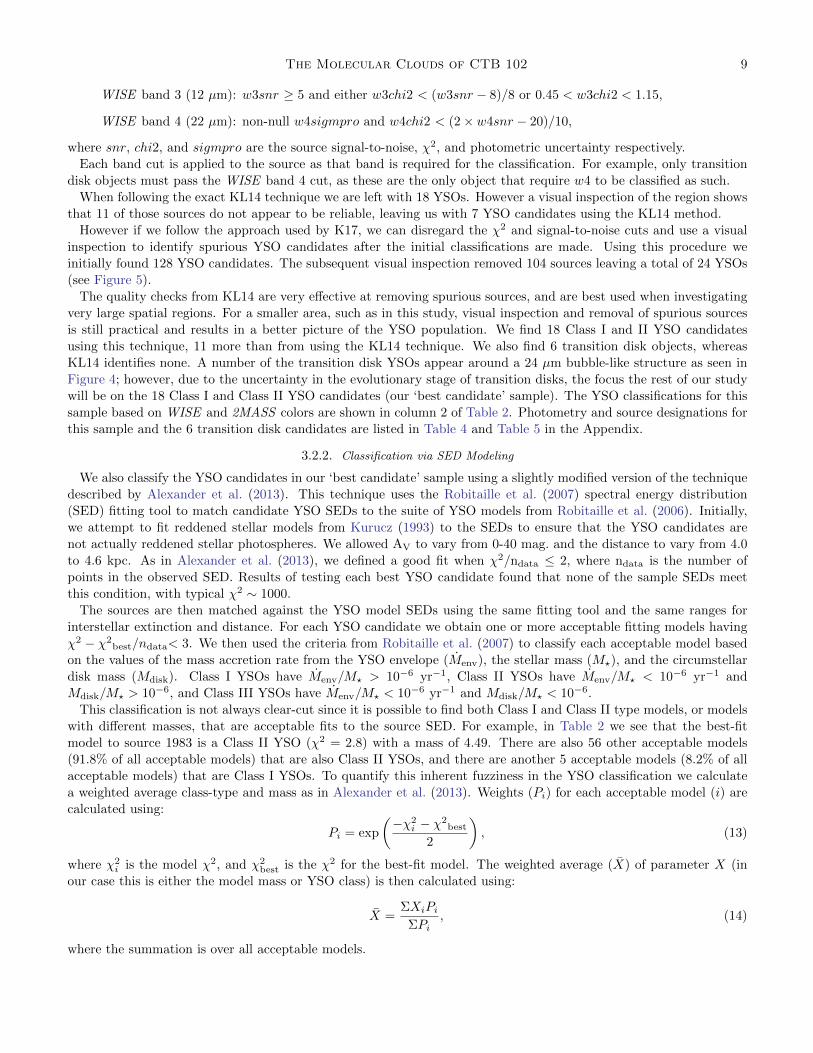
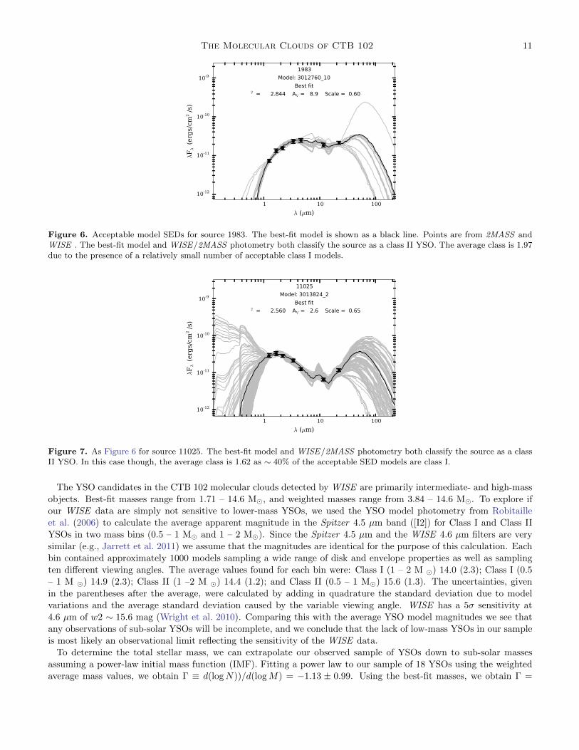
more detail. The best-fit and acceptable model SEDs are shown in Figure 6 and Figure 7. In the case of source 1983,

we find an average YSO class of 1.97, which reflects the fact that almost all of the acceptable models are Class II. The

weighted average mass of 4.41 M� is also similar to the best-fit model mass of 4.49 M�. For source 11025, the best

SED classification is a class II YSO, but in this case 40% of the acceptable models have a class I SED. The average

YSO class of 1.62 reflects this mix of acceptable models. We also see that the weighted average mass of 4.53 M� is

different from the best-fit model mass of 5.45 M�. Since the average decimal class (column 8 in Table 2) provides a

quantitative measure of the uncertainty of any given classification we prefer to use it over the strict binary class I or

class II classification from the WISE colors.

We see in Table 2 that there is a slight trend in the average YSO classification depending on the region where the

YSO is located. Regions 1, 1a, 2a, 2b, and 2c have average YSO classifications of 1.77, 1.78, 1.48, 1.33, and 1.66,

respectively. We notice that the more evolved YSOs (class II) tend to be in region 1 whereas younger YSOs tend to

be found in region 2. This may be indicative of separate (sequential) generations of star formation, where regions 2a,

2b, and 2c are younger because they are located farther from the main H II region. We hesitate to make any stronger

statement on this point though due to the small sample sizes in regions 2a, 2b, and 2c. The SED analysis was also

performed with a fixed distance of 4.3 kpc rather than allowing the distance to vary ±.3 kpc during the fitting. We

found that fixing the distance had no appreciable difference in the average mass or class of the YSOs, and therefore

would not propagate into our analysis of the star formation efficiency.

3.3. Star Formation Efficiency

The Molecular Clouds of CTB 102 11

1 10 100

λ (µm)

10-12

10-11

10-10

10-9

λFλ (erg

s/cm

2/s)

1983

Model: 3012760_10

Best fit

χ2 = 2.844 AV = 8.9 Scale = 0.60

Figure 6. Acceptable model SEDs for source 1983. The best-fit model is shown as a black line. Points are from 2MASS andWISE . The best-fit model and WISE/2MASS photometry both classify the source as a class II YSO. The average class is 1.97due to the presence of a relatively small number of acceptable class I models.

1 10 100

λ (µm)

10-12

10-11

10-10

10-9

λFλ (erg

s/cm

2/s)

11025

Model: 3013824_2

Best fit

χ2 = 2.560 AV = 2.6 Scale = 0.65

Figure 7. As Figure 6 for source 11025. The best-fit model and WISE/2MASS photometry both classify the source as a classII YSO. In this case though, the average class is 1.62 as ∼ 40% of the acceptable SED models are class I.

The YSO candidates in the CTB 102 molecular clouds detected by WISE are primarily intermediate- and high-mass

objects. Best-fit masses range from 1.71 – 14.6 M�, and weighted masses range from 3.84 – 14.6 M�. To explore if

our WISE data are simply not sensitive to lower-mass YSOs, we used the YSO model photometry from Robitaille

et al. (2006) to calculate the average apparent magnitude in the Spitzer 4.5 µm band ([I2]) for Class I and Class II

YSOs in two mass bins (0.5 – 1 M� and 1 – 2 M�). Since the Spitzer 4.5 µm and the WISE 4.6 µm filters are very

similar (e.g., Jarrett et al. 2011) we assume that the magnitudes are identical for the purpose of this calculation. Each

bin contained approximately 1000 models sampling a wide range of disk and envelope properties as well as sampling

ten different viewing angles. The average values found for each bin were: Class I (1 – 2 M �) 14.0 (2.3); Class I (0.5

– 1 M �) 14.9 (2.3); Class II (1 –2 M �) 14.4 (1.2); and Class II (0.5 – 1 M�) 15.6 (1.3). The uncertainties, given

in the parentheses after the average, were calculated by adding in quadrature the standard deviation due to model

variations and the average standard deviation caused by the variable viewing angle. WISE has a 5σ sensitivity at

4.6 µm of w2 ∼ 15.6 mag (Wright et al. 2010). Comparing this with the average YSO model magnitudes we see that

any observations of sub-solar YSOs will be incomplete, and we conclude that the lack of low-mass YSOs in our sample

is most likely an observational limit reflecting the sensitivity of the WISE data.

To determine the total stellar mass, we can extrapolate our observed sample of YSOs down to sub-solar masses

assuming a power-law initial mass function (IMF). Fitting a power law to our sample of 18 YSOs using the weighted

average mass values, we obtain Γ ≡ d(logN))/d(logM) = −1.13 ± 0.99. Using the best-fit masses, we obtain Γ =

12 Marshall et al.

Table 2. YSO classifications for best candidate sample

Best Fit Alternate Fit Average

ID K17 Classc % Matchd Masse AV Classf Massg Classh Massi AV Region

#a Classb (χ2) (# of Models) (M�) (mag.) (χ2) (M�) (M�) (mag.)

871 Class II (W) I (1.5) 93.6% (137) 4.94 4.18 II (18.7) 4.38 1.00 4.03 3.8 2b

1205* Class I (W) I (5.7) 60.0% (51) 5.15 16.6 II (15.1) 11.7 1.01 6.56 18.2 2b

1983* Class II (W) II (2.8) 91.8% (56) 4.49 8.9 I (8.4) 3.60 1.97 4.41 8.4 2a

1988 Class II (M) II (26) 100% (15) 14.6 6.6 · · · · · · 2.00 14.60 6.6 1

2927* Class I (W) II (1.1) 91.0% (496) 5.14 26.3 I (1.2) 6.21 1.89 5.32 27.0 2c

3232 Class I (W) I (3.0) 69.2% (72) 1.71 15.8 II (4.4) 7.45 1.43 3.84 15.7 2c

3263* Class II (W) II (2.1) 98.2% (214) 5.49 9.6 I (16.5) 6.56 2.00 5.74 9.3 1a

3703 Class II (M) II (40) 100% (10) 6.89 8.2 · · · · · · 2.00 6.89 8.2 1

4446 Class I (W) II (7.7) 91.9% (204) 5.91 21.0 I (15.2) 6.70 2.00 6.49 25.5 1a

4692 Class II (M) I (13) 100% (4) 7.15 1.4 · · · · · · 1.00 7.01 1.0 2a

5183 Class I (M) II (21.8) 59.5% (25) 6.64 1.5 I (31) 1.10 1.97 6.44 2.2 1a

5549 Class I (W) II (0.5) 91.8% (529) 5.49 32.3 I (3.6) 0.17 1.99 5.81 31.7 1a

5665 Class II (M) II (28) 20.0% (11) 6.62 11.7 I (30) 2.89 1.77 5.82 9.3 1a

5938 Class II (M) I (42) 83.1% (64) 5.62 4.1 II (53.3) 5.98 1.00 5.05 3.7 1a

6879* Class I (W) II (3.3) 95.4% (267) 5.26 13.8 I (8) 4.92 1.99 6.24 12.1 · · ·7392* Class II (W) II (20.6) 82.5% (14) 4.16 2.3 I (35) 3.07 2.00 4.12 2.3 1

8309* Class II (W) I (33) 100% (10) 5.18 3.4 · · · · · · 1.00 5.19 3.4 1

11025 Class II (W) II (2.5) 60.0% (152) 5.45 2.6 I (4.2) 3.14 1.62 4.53 2.9 · · ·aAll sources were verified by eye; * sources also meet the photometry quality cuts from KL14.

bSource classification based on the criteria in K12, KL14, and K17. W denotes the classification was based solely onWISE data, and M denotes that 2MASS and WISE data were used.

cSource classification based on YSO models best fit to the source SEDs and classification scheme from Robitaille et al. (2006)and the χ2 of the fit.

dPercentage of good fit YSO models that are the same classification type as the best fit and the number of models that fit.

eStellar mass of best fit YSO model.

fThe classification of the best fit model with a different YSO class than the best fit along with the χ2 of the fit. In somecases alternate classifications are not present because each well fit model are the same class as the best fit.

gStellar mass of the alternative classification best fit YSO model.

hWeighted average decimal classification based on the χ2 for each good fit model.

i Weighted average mass for each good fit model.

0.012± 0.32. Both of these slopes are flatter than the canonical Salpeter (1955) IMF (Γ = −1.35), but we believe this

is due to the small number of YSOs in our sample.

To explore this further, we designed a simulation to observe how cluster size influences an observed IMF. This was

done by simulating clusters with four different underlying IMF slopes, Γ = −0.35, −0.85, −1.10, and −1.35, and stellar

masses ranging between 2 – 14 M� (the range of mass values in Table 2). For each different cluster IMF, we simulated

sample sizes of 3, 10, 18, 30, 100, 300, 1000, and 3000 YSOs. Each simulation was run 1000 times per sample size.

We found that the observed IMF slope does not approach the actual value until the sample reaches approximately 100

in size (see Figure 8). For very small YSO sample sizes, it is essentially impossible to get the true IMF slope from

the observations. For a Salpeter IMF, we find that a random selection of 18 YSOs will produce Γ = −0.38 ± 0.44,

matching within the errors of our observed IMF for the best fit YSOs (black square in Figure 8). We also see that our

The Molecular Clouds of CTB 102 13

0.0 0.5 1.0 1.5 2.0 2.5 3.0 3.5 4.0

Log N(YSOs)

−2.0

−1.5

−1.0

−0.5

0.0

0.5

1.0

Γ

Γ = −0.35

Γ = −0.85

Γ = −1.35

Γ = −1.10

Figure 8. Derived IMF slope Γ ≡ d(logN))/d(logM) as a function of simulated cluster size for clusters following differentunderlying IMFs. Red dots correspond to a cluster with an intrinsic Γ = −1.35, purple follow Γ = −1.10, blue follow Γ = −0.85,and green follow Γ = −0.35. Error bars correspond to the standard deviation of the simulated clusters. The black squarecorresponds to our observed IMF slope based on the best-fit YSO masses, and the cyan corresponds to the average mass values.

observed IMF is consistent with other power laws within the large standard deviation for small sample sizes, but we

find no reason to not follow Γ = −1.35 in estimating the cluster mass in our case. Using Γ = −1.35, we use the 6 – 7

M� YSOs from Table 2 in each region to normalize our IMF, and extrapolate down to the sub-solar mass regime to

determine the cluster mass.

The star formation efficiency (SFE), MCluster/(MCluster + MGas), was found by considering three different cluster

masses. We first look at only our sample of detected YSOs to determine the cluster masses within each region,

thus setting a lower limit of the SFE (SFEMin in Table 3). We also use the Salpeter IMF, with Γ = −1.35, for

0.5 M� ≤ M < M�,Max = 7 M� and Γ = 0 for 0.08 M� < M < 0.5 M� (SFE in Table 3) . Finally, we derived an

alternative cluster mass using the same IMF, but ignoring YSOs with M < 0.5 M� (SFEAlt. in Table 3).

Table 3 shows our calculated star formation efficiencies for each of the subdivided regions and in total. We remind

the reader that systematic effects discussed in subsection 3.1, which we believe are small in this case, may result in

the SFE values being overestimated.

4. DISCUSSION

The molecular clouds associated with CTB 102 are likely the substantial remnants of an even larger initial GMC

that was the birthplace of CTB 102. They are 60× 35 pc in extent, and our 13CO observations provide a lower limit

mass estimate of 104.07 M�, while our 12CO observations give a mass range of 104.8 − 105.0 M�.

We used archival WISE and 2MASS photometry to identify and classify 18 class I and class II YSOs within the

molecular clouds. SED fitting was used to estimate YSO masses and to refine the YSO classifications. Star formation

activity is not spread uniformly throughout the clouds, rather our study reveals pockets of intermediate-mass star

formation, closely associated with the high 12CO and 13CO concentrations seen in Figure 1 and Figure 4. The lack of

observed low-mass YSOs (M < 2 M�) is very likely a selection effect due to the sensitivity of the WISE bands and

the distance of the molecular cloud.

14 Marshall et al.

Table 3. Cluster Mass and Star Formation Efficiency

Region 1 1a 2 2a 2b 2c Total

# of YSOs (Class I and II) 9 6 6 2 1 2 18

YSO Massa (M�) 75.2 35.5 27.2 11.4 6.6 9.2 108.2

SFEMin 0.4% 0.5% 0.07% 0.1% 0.06% 0.07% 0.18%

Cluster Mass (Log M�) 3.64 3.52 3.5 3.20 3.20 3.19 3.87

SFE (12CO)b 19.4% 33.9% 7.1% 13.7% 12.1% 10.1% 11.1%

SFE (virial)c 10.5% 23.2% 5.8% 8.0% 8.7% 5.8% 7.8%

Alt. Cluster Mass (Log M�) 3.5 3.34 3.32 3.03 3.03 2.68 3.70

SFEAlt (12CO) 13.7% 25.3% 4.8% 9.7% 8.5% 3.4% 7.8%

SFEAlt (virial) 7.4% 16.6% 3.9% 5.6% 6.1% 1.9% 5.4%

aSum of average YSO masses in the region (see Table 2).

bStar formation efficiency based on the cluster mass and the 12CO mass.

cStar formation efficiency based on the cluster mass and the virial mass.

The average YSO classification depends on position within the molecular cloud. We found the average YSO class

for region 1 and 2 to be 1.74 and 1.47 respectively. This may be indicative of separate generations of star formation

potentially stemming from the O star(s) powering CTB 102. A stronger statement on the existence of an age/class

gradient is precluded because of the small YSO sample size: seven YSOs in region 2 and nine YSOs in region 1.

A number of transition disk objects were identified, and, although we do not study them in detail, we saw that they

appear in a region without any significant amount of 12CO or 13CO emission. Interestingly, the majority of them

instead appear associated with a bubble-like structure seen in the mid-infrared WISE wavelengths and at 1420 MHz

outside of regions 1 and 2c (see Figure 1 and Figure 2). Again, while the sample size is small, the spatial location

of these objects, which are presumably more evolved YSOs than class II objects, is consistent with the gradient in

age/class mentioned in the previous paragraph.

The total SFEMin of the CTB 102 molecular cloud is 0.18%, which is quite low. However, this is to be expected,

as the sensitivity of WISE keeps us from observing low-mass YSOs that are likely there. When we use the MCluster

values, derived using IMF extrapolations from the observed YSOs (see subsection 3.3), the total SFE and SFEAlt.

values increase and range between ∼ 5 – 10%. This range of SFE is only slightly higher than typical values found for

giant molecular clouds (GMCs) at this spatial scale; Evans et al. (2009) find the SFE of molecular clouds on the scale

of 10 – 70 pc2 to be between 3 – 6%, and Evans & Lada (1991) found the SFE of L1630 to be 3 – 4% over a 40× 60

pc region. Given the uncertainties involved with our estimates for the total stellar population, we believe our results

for the overall SFE of the CTB 102 molecular clouds are consistent with previous studies of GMCs.

We also examined the SFE of the various sub-regions of the molecular cloud, and found that most regions had SFEs

in the 2 – 10% range. Region 1a was a clear outlier, with a SFE of 17 – 35%, depending on the cluster and gas mass

determination technique used. These values are strikingly high for a ∼ 5 × 5 pc region, and they are more typically

associated with the SFE of dense cores on the sub-pc scale. For example, Lada (1992) finds that massive cores in

GMCs have a SFE between 30 – 40%, and Tachihara et al. (2002) calculated the SFE for a sample of 179 cores finding

an average SFE of ∼10%, with a values as high as 40%. We suggest that the 1a region could be an example of a

massive embedded protocluster. These objects have, by definition, a stellar density of ρ∗ > 1 M� pc−3, and region

1a has ρ∗ = 10 − 20 M� pc−3 using a third spatial dimension of 10 – 5 pc. They also have observed SFEs ranging

between 8 – 33%, with higher values apparently associated with more evolved clusters (Lada & Lada 2003). Perhaps

the best nearby (d < 2 kpc) analog, considering both SFE and spatial scale, would be the Mon R2 embedded cluster,

which has a 25% SFE over a 1.85 pc spatial scale (see Table 2 in Lada & Lada 2003).

5. CONCLUSIONS

The Molecular Clouds of CTB 102 15

In this paper we introduced the first high resolution 12CO and 13CO observations of the molecular clouds associated

with the enormous CTB 102 H II region, which were obtained using the recently commissioned SEQUOIA-TRAO

system. The conclusions of our study are summarized below:

1. We find that what remains of the original molecular cloud has separated into at least two main regions, as seen

by the strong divide in the 12CO and 13CO maps (see Figure 1), and contains a total mass of 104.8 − 105.0 M�.

2. The molecular cloud contains ongoing star formation as seen by the presence of 18 intermediate-mass YSOs

within the cloud. When comparing the pockets of star formation, we found that there is a difference in the average

YSO class between them, suggesting there are at least two separate generations of star formation.

3. The SFE of the molecular cloud as a whole is comparable with efficiencies found for other Galactic GMCs.

However, with a SFE between 17 and 37%, the region 1a SFE is much higher than what would be expected for a

region only 5× 5 pc in size, and we think the region is likely the site of an embedded massive protocluster.

We are grateful to the staff members of the TRAO who helped to maintain and operate the telescope and to correlate

the data. The TRAO is a facility operated by the KASI (Korea Astronomy and Space Science Institute).

This publication makes use of data products from the Wide-field Infrared Survey Explorer, which is a joint project

of the University of California, Los Angeles, and the Jet Propulsion Laboratory/California Institute of Technology,

and NEOWISE, which is a project of the Jet Propulsion Laboratory/California Institute of Technology. WISE and

NEOWISE are funded by the National Aeronautics and Space Administration.

This publication makes use of data products from the Two Micron All Sky Survey, which is a joint project of

the University of Massachusetts and the Infrared Processing and Analysis Center/California Institute of Technology,

funded by the National Aeronautics and Space Administration and the National Science Foundation.

Miju Kang was supported by Basuc Science Research Program through the National Research Foundation of Ko-

rea(NRF) funded by the Ministry of Science, ICT & Future Planning (No. NRF-2015R1C2A1A01052160).

APPENDIX

WISE and 2MASS photometric data for our best YSO candiate sample and for the transition disk candidates are

provided in Table 4 and Table 5 respectively.

REFERENCES

Alexander, M. J., Kobulnicky, H. A., Kerton, C. R., &

Arvidsson, K. 2013, ApJ, 770, 1

Arvidsson, K., Kerton, C. R., & Foster, T. 2009, ApJ, 700,

1000

Baudry, A., Lucas, R., & Guilloteau, S. 1995, A&A, 293,

594

Blake, G. A., Sutton, E. C., Masson, C. R., & Phillips,

T. G. 1987, ApJ, 315, 621

Bolatto, A. D., Wolfire, M., & Leroy, A. K. 2013, ARA&A,

51, 207

Brand, J., & Blitz, L. 1993, A&A, 275, 67

Clark, P. C., & Glover, S. C. O. 2015, MNRAS, 452, 2057

Evans, II, N. J., & Lada, E. A. 1991, in IAU Symposium,

Vol. 147, Fragmentation of Molecular Clouds and Star

Formation, ed. E. Falgarone, F. Boulanger, & G. Duvert,

293

Evans, II, N. J., Dunham, M. M., Jørgensen, J. K., et al.

2009, ApJS, 181, 321

Ferland, G. J., Chatzikos, M., Guzman, F., et al. 2017,

RMxAA, 53, 385

Fitzgerald, M. P. 1968, AJS, 73, 177

Gong, M., Ostriker, E. C., & Kim, C.-G. 2018, ApJ, 858, 16

Heyer, M. H., Brunt, C., Snell, R. L., et al. 1998, ApJS,

115, 241

Jackson, J. M., Rathborne, J. M., Shah, R. Y., et al. 2006,

ApJS, 163, 145

Jarrett, T. H., Cohen, M., Masci, F., et al. 2011, ApJ, 735,

112

Kallas, E., & Reich, W. 1980, A&AS, 42, 227

Kang, S.-J., Kerton, C. R., Choi, M., & Kang, M. 2017,

ApJ, 845, 21

Koenig, X. P., & Leisawitz, D. T. 2014, ApJ, 791, 131

Kurucz, R. L. 1993, VizieR Online Data Catalog, 6039

Lada, C. J., & Lada, E. A. 2003, ARA&A, 41, 57

Lada, E. A. 1992, ApJL, 393, L25

Lynds, B. T. 1962, ApJS, 7, 1

16 Marshall et al.

Table 4. Best YSO Candidate Sample

WISEA ID # W1 W2 W3 W4 J H K Photometric Quality

Mag. Mag. Mag. Mag. Mag. Mag. Mag. Flags

J211338.41+522330.8 871 10.58 10.11 8.25 4.91 12.99 11.89 11.15 AAAA AAA

J211445.14+523407.2 1205 9.52 7.66 4.36 1.51 18.31 15.12 12.77 AAAA UUA

J211501.34+523548.3 1983 10.18 9.13 6.62 4.31 14.30 12.86 11.93 AAAA AAA

J211307.59+522534.4 1988 9.74 9.26 8.63 7.14 12.12 11.10 10.43 AAAU AAA

J211337.38+521446.8 2927 10.70 9.25 6.80 3.71 16.38 14.50 13.19 AAAA UUA

J211357.37+521250.9 3232 11.29 9.98 6.46 3.67 16.58 15.47 13.49 AAAA UCA

J211250.25+523018.8 3263 9.10 7.98 5.46 3.28 14.23 12.05 10.60 AAAA AAA

J211312.33+523739.4 3703 11.01 10.43 5.61 4.08 14.93 13.86 12.84 AAAA AAA

J211237.51+523150.4 4446 10.11 8.70 5.05 2.29 15.53 14.35 14.02 AAAA UUB

J211521.16+524050.0 4692 11.91 11.34 7.12 2.58 13.94 13.06 12.62 AAAA AAA

J211226.93+523051.5 5183 10.95 9.93 5.69 3.04 16.83 15.48 14.28 AAAA UBA

J211224.12+523139.3 5549 10.73 9.28 6.41 3.67 17.37 15.03 13.60 AAAA UUA

J211222.15+523113.5 5665 11.13 10.52 5.93 3.06 16.02 14.78 13.88 AAAA AAA

J211220.54+523147.3 5938 10.84 10.30 5.57 2.48 16.07 14.65 13.95 AAAA AAA

J211546.43+521102.3 6879 9.77 8.28 5.39 3.23 16.36 14.05 11.99 AAAA UAA

J211333.92+524623.4 7392 10.814 9.20 7.102 4.768 14.778 13.983 12.418 AAAA UAU

J211154.69+522825.5 8309 10.31 9.89 8.59 4.27 12.93 11.86 11.14 AAAA AAA

J211437.81+525154.1 11025 10.262 9.87 7.723 4.942 12.794 11.865 11.240 AAAA AAA

Table 5. Transition Disk Candidate Sample

WISEA ID # W1 W2 W3 W4 J H K Photometric Quality

Mag. Mag. Mag. Mag. Mag. Mag. Mag. Flags

J211448.55+523417.1 1299 8.493 8.2 7.539 5.077 13.07 10.379 9.171 AAAA AAA

J211225.28+522351.9 5151 8.331 8.158 7.945 5.144 10.559 9.55 9.009 AAAA AAA

J211152.50+522147.8 8876 9.338 8.95 7.959 4.873 11.693 10.729 10.082 AAAB AAA

J211151.18+522247.2 8885 7.874 7.549 6.906 4.813 10.225 9.326 8.736 AAAB AAA

J211203.64+521614.0 9079 8.958 8.795 9.167 6.091 10.933 10.075 9.582 AAAA AAA

J211144.96+522232.5 9697 8.044 7.683 6.898 4.172 10.071 9.221 8.657 AAAA AAA

Milam, S. N., Savage, C., Brewster, M. A., Ziurys, L. M., &

Wyckoff, S. 2005, ApJ, 634, 1126

Robitaille, T. P., Whitney, B. A., Indebetouw, R., & Wood,

K. 2007, ApJS, 169, 328

Robitaille, T. P., Whitney, B. A., Indebetouw, R., Wood,

K., & Denzmore, P. 2006, ApJS, 167, 256

Rohlfs, K., & Wilson, T. L. 2004, Tools of radio astronomy

Salpeter, E. E. 1955, ApJ, 121, 161

Simon, R., Jackson, J. M., Clemens, D. P., Bania, T. M., &

Heyer, M. H. 2001, ApJ, 551, 747

Simonson, S. C., I., & van Someren Greve, H. W. 1976,

A&A, 49, 343

Skrutskie, M. F., Cutri, R. M., Stiening, R., et al. 2006, AJ,

131, 1163

Szucs, L., Glover, S. C. O., & Klessen, R. S. 2016, MNRAS,

460, 82

Tachihara, K., Onishi, T., Mizuno, A., & Fukui, Y. 2002,

A&A, 385, 909

Taylor, A. R., Gibson, S. J., Peracaula, M., et al. 2003, AJ,

125, 3145

Whitney, B., Arendt, R., Babler, B., et al. 2008, Spitzer

Proposal, 60020

Wilson, R. W., & Bolton, J. G. 1960, PASP, 72, 331

Wright, E. L., Eisenhardt, P. R. M., Mainzer, A. K., et al.

2010, AJ, 140, 1868