the estimation of money demand in the slovak republic · the estimation of money demand in the...

C U R R E N T T O P I C

1volume 15, 8/2007

The estimation of money demandin the Slovak Republic

Ing. Viera Kollárová, Ing. Rastislav âárskyNational Bank of Slovakia

INTRODUCTION

This article focuses on the estimation of mon-ey demand and the identification of any mone-tary-policy implications. Money demand modelscan be suitable tools with which to assess mon-etary developments. A stable relationship be-tween money and the real economy should helpthe NBS to identify potential imbalances and in-flationary pressures.

To begin with, we select the individual variables,including the definition of money that is to beused. The description of the variables also in-

cludes an analysis of behaviour and economic sig-nificance in relation to money. The next part isdevoted to the econometric estimation of themoney demand function, and the final part fo-cuses on the econometric interpretation of theestimated parameters and the potential for us-ing the estimated equations to identify imbalancesin the economy.

SELECTION OF VARIABLES

Definition of moneyThe variable representing money demand was

Source: NBS.

Monetary aggregate M2 (1993 – 2006)

Source: NBS.

Contributions of individual M2 components to its year-on-year dynamics


2 volume 15, 8/2007

taken to be the M2 money supply, as defined inthe NBS methodology1 (until 2005). This variablewas selected because the monetary aggregatesin the ECB methodology have only been report-

ed since 2003 and it is not possible to back-cal-culate them. In order to have a longer time se-ries, the M2 money supply data were addition-ally calculated up to the present. Owing to dif-

ferent methodologies, small differences may arisein the description of individual components of themoney supply.

Economic activityThe variable that explains the relationship be-

tween money and economic activity is related tothe transaction motive for holding money. For this'scale variable', we selected real gross domesticproduct. We also considered, for example, retailturnover and industrial output, but these weredeemed statistically insignificant.

Given that motives for holding deposits differbetween sectors (corporate and household), thedevelopment of deposits share in GDP is alsodifferent. Whereas the corporate sector uses de-posits mostly to service its transactions, house-holds use them mainly as a form of saving. Thisis confirmed also by the differences in corporatedeposits and household deposits share in GDP.While the ratio of corporate deposits (around60% of which are demand deposits) is gradual-ly increasing, the ratio of household deposits isin a long-term decline.

Some household deposits are, however, also re-lated to the transaction motive for holding mon-ey and to economic activity, particularly in the caseof demand deposits, that is, deposits repayableon demand. The improving situation in the labourmarket, wage developments, and above all em-ployment growth, are gradually being reflectedin the dynamics of demand deposit growth, andthe ratio of these deposits to GDP is developingsimilarly to the ratio of corporate deposits. From2001 to the end of 2006, their ratio recorded analmost identical increase of between 3 and 5percentage points.

Source: NBS, Statistical Office of the Slovak Republic.

Deposits as a share in GDP (2001 – 2006)

Year-on-year increase in household deposits (in SKK bln) and growth in employment (according to labour force samplesurvey) and in wages (in %)

Household demand deposits as a share in GDP

Source: NBS.

Source: NBS, Statistical Office of the Slovak Republic.

1 Definition of monetary aggregates:M0 = currency in circulationoutside banks;M1= M0 + demand deposits andsavings deposits redeemablewithout a period of notice, heldby domestic non-banking entities(residents + non-residents, in SKK)vis- a-vis the domestic bankingsystem – excluding funds ofgovernment and local authoritybodies;M2 = M1 + time deposits andsavings deposits redeemable at aperiod of notice (residents + non-residents, non-banking entities),denominated in SKK and includingcertificates of deposit + foreigncurrency demand deposits andtime deposits (residents, non-banking entities) held vis- a-vis thedomestic banking system –excluding funds of governmentand local authority bodies.


3volume 15, 8/2007

Own yield of money and alternative assets(financial innovation)

Money is used not only as a medium of ex-change, but also, especially among households,as a form of saving. The variables that explain thebehaviour of deposits in regard to the savingmotives of economic entities are usually the ownyield of money or the yield of alternative assetsinto which savings may be allocated. As regardsthe type of deposits, the rate of return on indi-vidual assets should affect the behaviour of de-mand and savings deposits. If the own yield ofmoney rises in comparison with the yield of al-ternative assets, the demand for money shouldalso increase. Conversely, if the yield of alterna-tive assets rises, interest in deposits will decline.

To approximate own yield, we selected the to-tal interest rate on deposits of households andnon-financial corporations. The following chartindicates the relationship between the interest rateon deposits and the development of deposits.

Household deposits show the most sensitivity

to interest developments. Since 2000, the NBS hasbeen fixing the key interest rates (overnight ster-ilization rate, overnight refinancing rate, and thetwo-week repo tender limit rate). As the outlookfor inflation gradually improved, the NBS loweredits key rates right up to 2005. This saw a sharpdecline in interest on demand and savings depositsand consequently a decline in the use of thesetypes of deposit.

As well as own yield of money, the uptake ofdeposits also affects the rate of return on alter-native assets. The most accessible type of alter-native financial asset are shares/units of mutualfunds, whether money market funds or others,especially equity funds and bond funds (their ra-tio to the money supply currently stands at morethan 10%).2 Since a database of the returns onthese funds is not available, we treated theamount of money invested in them to be the vari-able of alternative assets. The time series are, how-ever, relatively short and are available only from2 0 0 4 .3 The following charts show that investments

Source: NBS.

Year-on-year increase in total deposits and the deposit interest rate

Source: NBS.

Time deposits of households and the deposit interest rate

2 In the estimation of the moneydemand function, money marketfunds represent the alternativeasset where money is defined asthe M2 aggregate, and where theM3 aggregate is used they areincluded in it.

3 Data on money market fund(MMF) shares are available on amonthly basis; data on shares/unitsof investment funds other thanMMF are only available on aquarterly basis.


4 volume 15, 8/2007

in mutual funds (especially money market funds)are used relatively flexibly as an alternative to de-posits and react to changes in the returns on de-posits.

The role of mutual funds as a substitute for de-posits and the effect of deposit interest on thetransfer of funds between each type of financialasset are also recorded by the ratios of depositsand mutual funds, or rather the aggregate of bothof these products, to GDP. When interest de-creased, the ratio of deposits to GDP fell, and theratio of stocks and mutual fund shares rose. Theaggregate ratio (of household deposits,shares/units of mutual funds) to GDP, i.e. thehousehold savings rate in the economy, has re-mained constant with a slight decline in the pre-vious period. That, however, may have beencaused by the strong GDP growth in 2006.

The own yield of money is included in thelong-run money demand equation, althoughconsidering the shortness of the time series formutual funds, the variable describing the devel-opment of alternative assets vis- a-vis deposits isonly included in the short-run part of the equa-tion (in the long-run it is not significant).

Price levelIn studies of money demand, the price level is

usually measured with the implicit deflator ofGDP, the consumer price index or the producerprice index. In this case, the selected deflatorwas the harmonized index of consumer prices ad-justed for the effects of prices of energy and un-processed food.

SeasonalityFor modelling, we also applied seasonality ex-

pressing the increase in the money supply in thefourth quarter. This rise is caused by the factthat deposit interest is always credited at theend of the year.

Year-on-year growth in household deposits and mutual fundshares/units

Year-on-year growth in household deposits and mutual fundshares/units

Source: NBS.

Source: NBS, Statistical Office of the Slovak Republic.Note: Mutual fund shares are the sum of money market fund (MMF) shares/units and shares/units of investment funds other than MMF,as reported since 2004.

Source: NBS.

Deposits and mutual funds as a share in GDP


5volume 15, 8/2007

ECONOMETRIC ANALYSIS

The money demand model was created onthe basis of quarterly data, running from the 1stquarter of 2000 to the 4 quarter of 2006. The es-timation does not date further back, because ofthe structural break in the character of the mon-etary-policy environment. Up to 1998, the NBSused a fixed exchange rate regime within a fluc-tuation band. This was gradually broadened from±0.5% in 1993 to ±7.5%. Under the conditions ofa fixed exchange rate, the effectiveness of mon-etary policy is limited and volatility may, by meansof net foreign assets, be introduced into the de-velopment of monetary aggregates. In October1998, the NBS abandoned the fixed rate regime,and in 1999 the economic environment report-ed gradual stabilization based on both, devalu-ation of the exchange rate and economic-policymeasures. From 2000, the conduct of monetarypolicy shifted from quantitative implementation,

to qualitative implementation through the fix-ing of key interest rates – today's dominant toolof monetary policy. The previous period also sawcertain changes in the monetary-policy environ-ment, one being the introduction of inflationtargeting (since 2005) and the other being en-try into ERM II (in November 2005).

The length of the time series may considerablyaffect the scope for modelling money demand.All the variables used in the model are real, de-flated by the HICP (excluding energy and un-processed food). The estimation of the money de-mand function is made using two approaches: thePartial Adjustment Model (PAM) and the VectorError Correction Model (VECM).

1. Partial Adjustment ModelIt was decided to use several tools for the

econometric analysis of money demand. The firstof these is the partial adjustment model, throughwhich the long-run equilibrium and short-run

Foreign currency deposits of households and non-financial corporations expressed in SKKbillion and the exchange rate SKK/EUR

Source: NBS, Eurostat.

FOREIGN CURRENCY DEPOSITS

The M2 definition of money used in modellingthe money demand function presents a p a r t i c-ular problem in the form of foreign currency de-posits. These deposits are partially related totransaction requirements, especially in the caseof corporate deposits, but they can simultane-ously fulfil a savings function (such holdings maybe partially speculative) which is more commonfor household deposits. If the SK K ’s exchange rateappreciates, the accounts value of foreign cur-rency deposits declines and these deposits be-come less attractive given the expected loss(exchange rate). Such behaviour is most clearlydisplayed by household deposits, which were inan almost continuous decline until the end of2005. This trend ceased in the last period.

By contrast, corporate deposits reacted onlyslightly to exchange rate developments, witha more marked reaction observed at the begin-ning of 2005. Despite the relatively volatile de-velopment, there is an apparent rising trendwhich is probably related to the increasing open-ness of the economy and the development offoreign trade.

The antagonistic trends in foreign currency de-posits make it difficult to define a variable thatexplains their development. In seeking sucha variable for the estimation of money demand,we tested economic openness and the exchangerate, but neither of them provided to be statis-tically significant.


6 volume 15, 8/2007

4 ADF – Augmented Dickey-FullerUnit Root Test.

adjustment may be presented. We begin with thefollowing adjustment equation:

The long-run money demand equation is as fol-lows:

By means of a simple adjustment, we obtainthe short-run equation that will include real mon-ey supply with a time lag,

where:M2 is the money supply (lm2_rep);P is the HICP excluding energy and unprocessedfoodstuffs;Y is real GDP (lhdpsc);i is the real interest rate on deposits (lirt_rep)γ – is the adjustment coefficient.

EstimationTo the short-run equation there was added

the variable lplpf_rep (representing stocks andmutual fund shares/units) and @ s e a s ( 4 ) ( e x p r e s s-ing seasonality). The model was estimated usingthe least squares method and the result is as fol-lows (t-statistics are stated in brackets under thevariable):

LM2_REP = -3.0245 + 0.3666*LHDPSC [-2.9141] [5.5308]

+ 0.8263*LIRT_REP + 0.5791*LM2_REP(-1)[4.1119] [6.9665]

- 0.0196*LPLPF_REP + 0.0344*@SEAS(4)[-2.9262] [4.5739]

R-squarted 0,9302 F-statistic 56,0080Durbin-Watson stat 1,9963

The estimation results refer to the positive elas-ticity of the money supply relative to GDP as wellas the deposit interest rate. The statistical signif-icance of stocks and mutual fund shares/units wasalso confirmed – the fact that their elasticity is neg-ative confirms the hypothesis of substitution be-tween them and household deposits. Our mod-el also used a dummy variable representing sea-sonality, according to which the amount of theM2 money supply increased by 0.03% in thefourth quarter. This rise is probably caused by thecrediting of deposit interest at the year-end. Themodel is also suitable for predicting the develop-ment of the money supply (as confirmed by ananalysis using the CUSUM curve), although theforecasts may be slight overestimated. The mon-ey demand function is moderately unstable, asexpressed by recursive estimations of the mod-el's individual coefficients.

Based on the short-run and long-run equa-tion, the adjustment coefficient γ may be ex-pressed. This coefficient expresses the degree ofadjustment of real money balances vis- a-vis thelong-run equilibrium in the current period. Inour case, the adjustment is equal to 0.42. As withthe adjustment coefficient, equations can beused to express the long-run elasticity of M2 inrelation to each variable.

The long-run money demand equation:

The description of long-run elasticities will beaddressed at the end, along with the elasticitiesquantified with the estimation of the VECM model.

2. Vector Error Correction Model (VECM)The VECM is the second approach used in

modelling money demand. Under this approach,the simultaneous effect of all three variables(M2, GDP, deposit interest rate) on each other isestimated and the result is given as three equa-tions. The result represents an estimation of thestationary time series. Each of the model's vari-ables was tested for stationarity using the ADFtest,4 which found that they are non-stationaryand integrated of the same order I(1).

Given that the other equations (estimation ofGDP and the interest rate) have a low adjustmentcoefficient and the centre of our attention is themoney supply, these equations are not usedhereafter. The final estimated equation for M2is given as follows (t-statistics are stated in brack-ets under each variable):

D(LM2_REP) = - 0.3735 * (LM2_REP(-1) [-2.1239]

- 0.8238 * LHDPSC(-1) - 1.5852 * LIRT_REP(-1)[-6.1003] [-6.0445]

+ 5.1818 - 0.4184 * D( LM2_REP (-1)) [3.5791] [-2.7348]

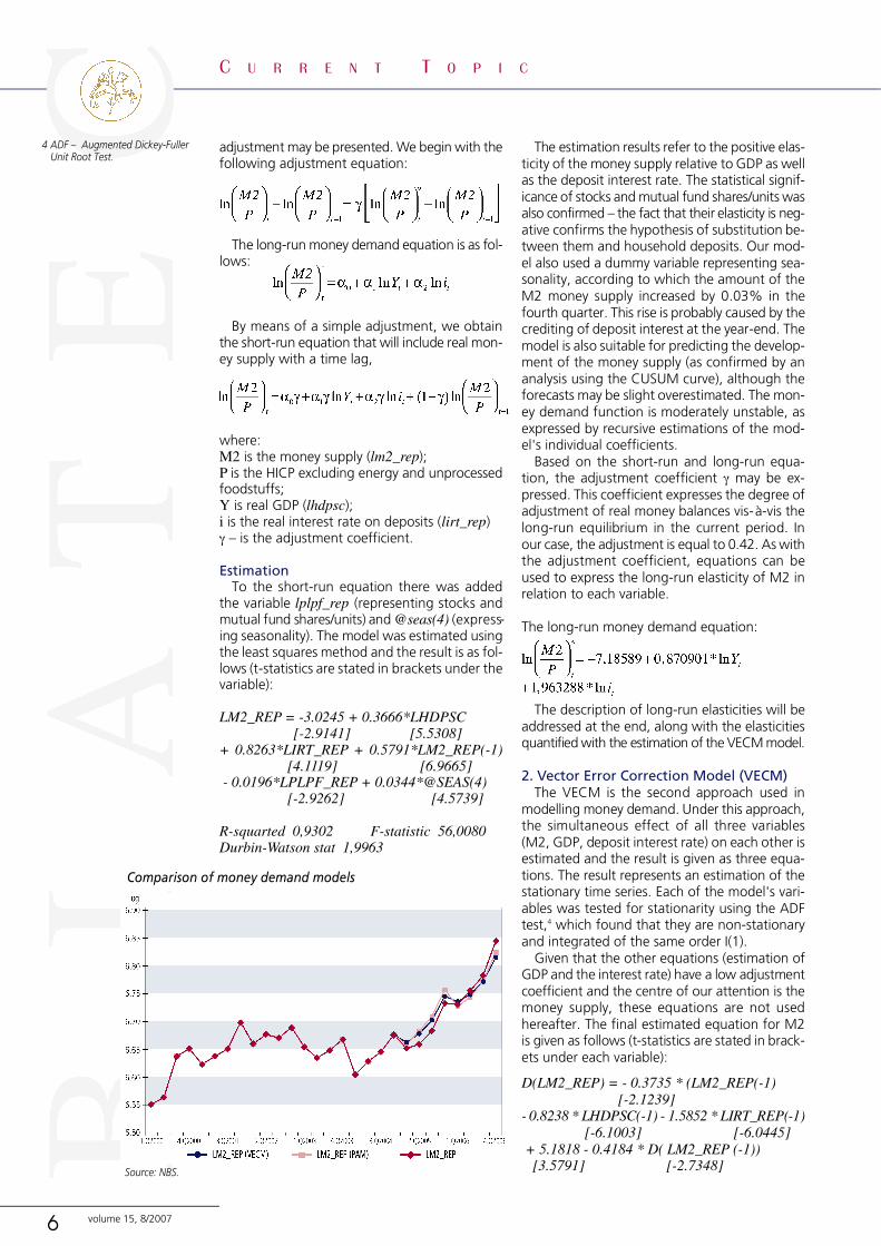
Comparison of money demand models

Source: NBS.


7volume 15, 8/2007

ed restructuring of selected banks and their pri-vatization. In 2000, meanwhile, the NBS beganthe reporting of key interest rates and therebyshifted from a quantitative to qualitative imple-mentation of monetary policy. Following a peri-od in which deposits attracted very high interest(nominal interest rates were averaging 10% in1998 and 1999), there was a relatively sharp de-cline in interest rates and so deposits became rel-atively less attractive, too. In this environment,households led the way in looking for alternativeforms of saving.

MONEY DEMAND ANDTHE IDENTIFICATION OF IMBALANCES

The difference between the equilibrium valuesof real M2, estimated from the long-run moneydemand equations and actual developments inthe M2 aggregate (at constant prices), is knownas the ’real money gap’. Its presence may signalthe potential emergence of imbalances, assum-ing, however, that the money demand functionis stable. In our case, this assumption is not ful-ly met. At the same time, the long-run equationdoes not include the variable of alternative assets(mutual funds), which for our purposes is crucialto the modelling of the money demand functionand was excluded from the long-run equationonly because of the shortness of the time series.If the short-run money demand equation lackedthis variable, it would also fail to give satisfacto-ry results. For that reason, we calculated the realmoney gap as the difference between the actu-al stock of real M2 and the real M2 estimatedfrom the short-run equation. The following iden-tification and interpretation of the real money gapis therefore only for guidance.

A comparison of the ex post values of the realmoney supply and the values simulated with thepartial adjustment model shows substantial dif-ference in only three periods. The most substan-tial difference was identified at the end of 2001and beginning of 2002, when the actual M2value significantly exceeded the simulated values.

+ 0.1135 * D (LHDPSC (-1)) + 0.0783[0.9277]

* D (LIRT_REP (-1)) - 0.0097 * LPLPF_REP[0.1661] [-1.3620]

+ 0.0273 * @SEAS(4)[2.8635]

When designing the models, we considered var-ious model specifications and various variables (in-flation, gross output, 3-month BRIBOR). Duringthe modelling, however, these were shown to bestatistically insignificant, or rather their parame-ters had signs opposite to those we had expect-ed on the basis of theory.

The two approaches presented here are themodels with the best estimation results, that is,with the most accurate estimation based on dy-namic forecasts generated ex post. This is alsorecorded by the chart for the period of the last8 quarters (the chart also shows the logarithmsof the values).

PARAMETERS OF LONG-RUN EQUATIONSAND THEIR INTERPRETATION

In both approaches, the long-run elasticities arerelatively similar, and as regards GDP, practical-ly identical. The VECM model indicates money de-mand reacts more strongly to interest rates. Theadjustment coefficients report approximately thesame figures and are comparable with estimatesmade in the past.5

The long-run elasticity relative to GDP is low-er than one, which indicates an increasing veloc-ity of money in circulation. This result does notcompletely coincide with the analysis of transac-tion deposits under M2, which we looked at inthe introductory part in the section on econom-ic activity. By contrast, the rising ratio of corpo-rate deposits and household demand deposits rel-ative to GDP could indicate elasticity closer to, orslightly higher than, one.

One reason why the long-run elasticity of thescale variable is lower than one could be the factthat the short-run part of the equation includes thevariable representing alternative assets from 2004,or that the long-run equation does not include thisfigure at all (shortness of the time series).

The absence of this variable may also be acause of the relatively high long-run elasticity oflong-run money demand in relation to own yieldof money. In both equations it is substantiallyhigher than one. That level, however, probablyalso reflects the monetary environment andprocesses taking place in the banking sector. Inaddition, the period for which we estimated thedemand function was influenced by the complet-

Variable6 PAM VECMln Y 0.8709 0.8238ln i 1.9633 1.5852Adjustment coefficient 0.4209 0.3735

Actual stock of real M2 and PAM-simulated values

Source: NBS

5 âársky R., Gavura M.: Modellingthe money demand function inSlovakia; Biatec 11, 1997.

6 The following variables are used:Y = real GDP;i = real deposit interest rate;adjustment coefficient = thedegree of adjustment of realmoney balances vis- a-vis the long-run equilibrium in the currentperiod


8 volume 15, 8/2007

A factor in the money supply growth was the ma-turity in 2001 of bonds issued by the NationalProperty Fund in a second wave of coupon pri-vatization. This effect was reflected to lesser ex-tent in subsequent quarters, and the M2 aggre-gate made a relatively quick return to equilibri-um. Another difference in comparison with thereal M2 was seen in the first quarter of 2004. Thiswas related to an administrative change of 31 De-cember 2003, when anonymous deposits wereabolished as required under the harmonizationof Slovak law with EU legislation.

A relatively long-run negative real money gap,in other words, a situation in which the actualstock of real M2 fluctuated below the simulatedvalues, was recorded in 2005. It may have beena sign that money was at this time having asomewhat dampening effect on prices. Tests ofthe function's quality in terms of forecasting abil-ity indicate, however, a slight tendency to over-estimate (CUSUM test).

In 2006, by contrast, the gap between thesimulated and actual values indicates that the ef-fect of money may be inflationary. This deviationis, however, low and falls within the margin oferror for generated forecasts (± 2* the standarddeviation of the estimation). Even so, the causecould as well be the strong economic growth(8.3% for 2006) and the increase in interest ratesduring the year; the main reaction to this camefrom households, with an increase in deposits andso-called ’portfolio shifts’7, which affected themoney supply but not price developments.

Using the VECM model to compare the actu-al stock of real M2 and simulated values indicatesthat from 2000 to 2003 there was a long-run, en-during surplus of money in comparison with themoney demand estimation. No satisfactory inter-pretation has been found for this gap. It came toan end in 2004, i.e. in the period when the vari-able of alternative assets join the function. Thisgap may have been caused by alternative mon-ey holdings (mutual funds shares/units) not be-ing taking into account, and therefore the mon-ey demand function estimated by the VECMmethod appears to be less suitable for the iden-tification of money market imbalances.

A comparison between gaps in the moneymarket (difference between actual stock of realmoney balances and estimated money demand)and the output gap8 indicates a similar develop-ment, although the levels do not correspond en-tirely. In 2000-2001, for example, when the out-put gap closed slightly, the positive real moneygap widened. Conversely, the negative output gapincreased in 2002-2003, accompanied by a nar-rowing of the positive real money gap. Since2005, both the development and level of gapsin the money market and the output gap havebegun to correspond.

CONCLUSION

Given the instability of the money demandfunction, its utilization for monetary-policy pur-poses is limited. The similar development of theoutput gap and real money gap only points to therequirement for money to service economic ac-tivity. If the overheating of economy were to beaffected by a relative surplus of money, thereshould be a certain lag between the real moneygap and output gap. The analysis did not, how-ever, indicate such a relationship.

For the moment, therefore, the estimated mon-ey demand function may be used as an alterna-tive/supplementary analytical tool for identify-ing potential imbalances in the economy, or forforecasting purposes.

Actual stock of real M2 and VECM-simulated values

Source: NBS

Output gap and real money gap

Source: NBS

Bibliography:1. ARTL, J., GUBA, M., RADKOVSK¯, ·., SOJKA, M., STILLER, V.:

Influence of Selected Factors on the Demand for Money 1994-2000; WP No. 30, Prague 2001.

2. BRAND. C., CASSOLA. N.: A Money Demand System for EuroArea M3, ECB, Working Paper No. 39, November 2000.

3. âÁRSKY. R., GAVURA. M.: Modelling the money demandfunction in Slovakia; Biatec no. 11, 1997.

4. DREGER. CH., REIMERS. H. E., ROFFIA. B.: Long-run Money

Demand in the New EU Member States with Exchange RateEffects, ECB, Working Paper No.628, May 2006.

5. KOMÁREK. L., MELECK . M.: Demand for Money in the TransitionEconomy: The Case of the Czech Republic 1993 – 2001, Warwickeconomic research papers No. 614, December 2001.

6. KUIJS. L.: Monetary Policy Transmission Mechanisms andInflation in the Slovak Republic, IMF, WP/02/80, May 2002.

7. VANCE. L. Martin: IMF Course: Basic Econometrics UsingEviews, November 2004.

7 Portfolio shifts – movementsbetween individual componentsand counterparts of the M3money supply and shares/units ofinvestment funds other than MMF.

8 The output gap is calculated onthe basis of the NBS model MVF-UC (Multivariate Filter withUnobserved Components); theestimation includes the deviationof inflation from its target, whichdetermines the development andsize of the gap.

the estimation of money demand in the slovak republic · the estimation of money demand in the...

Documents