The Cutting Plane Method is Polynomial for Perfect Matchings∗

Karthekeyan Chandrasekaran1, Laszlo A. Vegh2, and Santosh S. Vempala1

1College of Computing, Georgia Institute of Technology2Department of Management, London School of Economics

karthe, vempala@cc.gatech.edu, l.vegh@lse.ac.uk

Abstract

The cutting plane approach to optimal matchings has been discussed by several authors overthe past decades [22, 15, 18, 26, 11], and its convergence has been an open question. We provethat the cutting plane approach using Edmonds’ blossom inequalities converges in polynomialtime for the minimum-cost perfect matching problem. Our main insight is an LP-based methodto retain/drop candidate cutting planes. This cut retention procedure leads to a sequence ofintermediate linear programs with a linear number of constraints whose optima are half-integraland supported by a disjoint union of odd cycles and edges. This structural property of theoptima is instrumental in finding violated blossom inequalities (cuts) in linear time. Further,the number of cycles in the support of the half-integral optima acts as a potential function toshow efficient convergence to an integral solution.

1 Introduction

Integer programming is a powerful and widely used approach to modeling and solving discreteoptimization problems [20, 23]. Not surprisingly, it is NP-complete and the fastest known algorithmsare exponential in the number of variables (roughly nO(n) [17]). In spite of this intractability,integer programs of considerable sizes are routinely solved in practice. A popular approach is thecutting plane method, proposed by Dantzig, Fulkerson and Johnson [8] and pioneered by Gomory[12, 13, 14]. This approach can be summarized as follows:

1. Solve a linear programming relaxation (LP) of the given integer program (IP) to obtain abasic optimal solution x.

2. If x is integral, terminate. If x is not integral, find a linear inequality that is valid for theconvex hull of all integer solutions but violated by x.

3. Add the inequality to the current LP, possibly drop some other inequalities and solve theresulting LP to obtain a basic optimal solution x. Go back to Step 2.

∗This work was supported in part by NSF award AF0915903. This work was done while the second author wasaffiliated with the College of Computing, Georgia Institute of Technology, supported by NSF Grant CCF-0914732.

1

For the method to be efficient, we require the following: (a) an efficient procedure for finding aviolated inequality (called a cutting plane), (b) convergence of the method to an integral solutionusing the efficient cut-generation procedure and (c) a bound on the number of iterations to conver-gence. Gomory gave the first efficient cut-generation procedure and showed that the the cuttingplane method implemented using his cut-generation procedure converges to an integral solution [14].There is a rich theory on the choice of cutting planes, both in general and for specific problemsof interest. This theory includes interesting families of cutting planes with efficient cut-generationprocedures [12, 1, 4, 2, 5, 21, 3, 19, 25], valid inequalities, closure properties and a classificationof the strength of inequalities based on their rank with respect to cut-generating procedures [6](e.g., the Chvatal-Gomory rank [4]), and testifies to the power and generality of the cutting planemethod.

To our knowledge, however, there are no polynomial bounds on the number of iterations toconvergence of the cutting plane method even for specific problems using specific cut-generationprocedures. The best bound for general 0-1 integer programs remains Gomory’s bound of 2n [14].It is possible that such a bound can be significantly improved for IPs with small Chvatal-Gomoryrank [11]. A more realistic possibility is that the approach is provably efficient for combinatorialoptimization problems that are known to be solvable in polynomial time. An ideal candidate couldbe a problem that (a) has a polynomial-size IP-description (the LP-relaxation is polynomial-size),and (b) the convex-hull of integer solutions has a polynomial-time separation oracle. Such a problemadmits a polynomial-time algorithm via the Ellipsoid method [16]. Perhaps the first such interestingproblem is minimum-cost perfect matching: given a graph with costs on the edges, find a perfectmatching of minimum total cost.

A polyhedral characterization of the matching problem was discovered by Edmonds [9]: Basicsolutions of the following linear program (extreme points of the polytope) correspond to perfectmatchings of the graph.

min∑uv∈E

c(uv)x(uv) (P)

x(δ(u)) = 1 ∀u ∈ Vx(δ(S)) ≥ 1 ∀S ( V, |S| odd, 3 ≤ |S| ≤ |V | − 3

x ≥ 0

The relaxation with only the degree and nonnegativity constraints, known as the bipartite relaxation,suffices to characterize the convex-hull of perfect matchings in bipartite graphs, and serves as anatural starting relaxation. The inequalities corresponding to sets of odd cardinality greater than 1are called blossom inequalities. These inequalities have Chvatal rank 1, i.e., applying one round ofall possible Gomory cuts to the bipartite relaxation suffices to recover the perfect matching polytopeof any graph [4]. Moreover, although the number of blossom inequalities is exponential in the sizeof the graph, for any point not in the perfect matching polytope, a violated (blossom) inequalitycan be found in polynomial time [22]. This suggests a natural cutting plane algorithm (Figure 1),proposed by Padberg and Rao [22] and discussed by Lovasz and Plummer in their classic book onmatching theory [18]. Experimental evidence suggesting that this method converges quickly wasgiven by Grotschel and Holland [15], by Trick [26], and by Fischetti and Lodi [11]. It has been opento rigorously explain their findings. In this paper, we address the question of whether the methodcan be implemented to converge in polynomial time.

2

The known polynomial-time algorithms for minimum-cost perfect matching are variants of Ed-monds’ weighted matching algorithm [9]. It is perhaps tempting to interpret the latter as a cuttingplane algorithm, by adding cuts corresponding to the shrunk sets in the iterations of Edmonds’algorithm. However, there is no correspondence between the solution x of the LP given by non-negativity and degree constraints and a family F of blossom inequalities, and the partial matchingM in the iteration of Edmonds’ algorithm when F is the set of shrunk nodes. In particular, thenext odd set S shrunk by Edmonds’ algorithm might not even be a cut for x (i.e., x(δ(S)) ≥ 1).It is even possible, that the bipartite relaxation already has an integer optimal solution, whereasEdmonds’ algorithm proceeds by shrinking and unshrinking a long sequence of odd sets.

1. Start with the bipartite relaxation.

2. While the current solution is fractional,

(a) Find a violated blossom inequality and add it to the LP.

(b) Solve the new LP.

Figure 1: Cutting plane method for matchings

The bipartite relaxation has the nice property that any basic solution is half-integral and itssupport is a disjoint union of edges and odd cycles. This makes it particularly easy to find violatedblossom inequalities – any odd component of the support gives one. This is also the simplestheuristic that is employed in the implementations [15, 26] for finding violated blossom inequalities.However, if we have a fractional solution in a later phase, there is no guarantee that we can findan odd connected component whose blossom inequality is violated, and therefore sophisticated andsignificantly slower separation methods are needed for finding cutting planes, e.g., the Padberg-Raoprocedure [22]. Thus, it is natural to wonder if there is a choice of cutting planes that maintainshalf-integrality of intermediate LP optimal solutions.

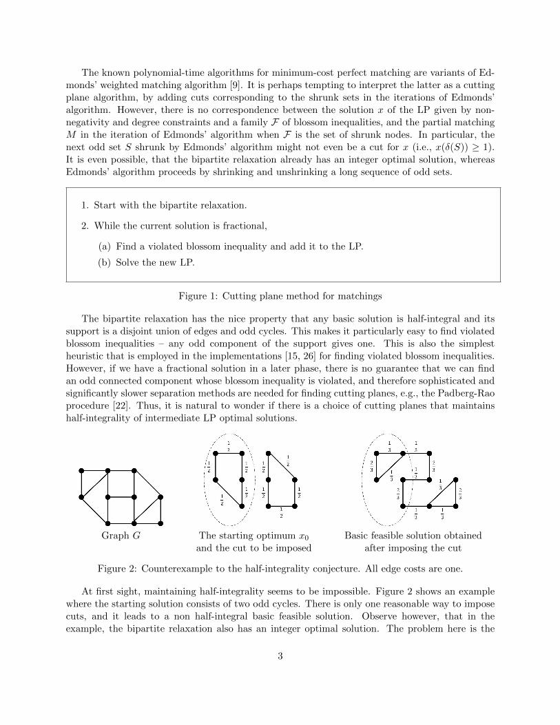
Graph G The starting optimum x0 Basic feasible solution obtainedand the cut to be imposed after imposing the cut

Figure 2: Counterexample to the half-integrality conjecture. All edge costs are one.

At first sight, maintaining half-integrality seems to be impossible. Figure 2 shows an examplewhere the starting solution consists of two odd cycles. There is only one reasonable way to imposecuts, and it leads to a non half-integral basic feasible solution. Observe however, that in theexample, the bipartite relaxation also has an integer optimal solution. The problem here is the

3

existence of multiple basic optimal solutions. To avoid such degeneracy, we will ensure that alllinear systems that we encounter have unique optimal solutions.

This uniqueness is achieved by the simple deterministic perturbation of the integer cost function,which increases the input size polynomially. We observe that this perturbation is only a first steptowards maintaining half-integrality of intermediate LP optima. More careful cut retention andcut addition procedures are needed to maintain half-integrality.

1.1 Main result

To state our main result, we first recall the definition of a laminar family: A family F of subsetsof V is called laminar, if for any X,Y ∈ F , one of X ∩ Y = ∅, X ⊆ Y , Y ⊆ X holds.

Next we define a perturbation to the cost function that will help avoid some degeneracies. Givenan integer cost function c : E → Z on the edges of a graph G = (V,E), let us define the perturbationc by ordering the edges arbitrarily, and increasing the cost of edge i by 1/2i.

We are now ready to state our main theorem.

Theorem 1.1. Let G = (V,E) be a graph on n nodes with edge costs c : E → Z and let c denotethe perturbation of c. Then, there exists an implementation of the cutting plane method that findsthe minimum c-cost perfect matching such that

(i) every intermediate LP is defined by the bipartite relaxation constraints and a collection ofblossom inequalities corresponding to a laminar family of odd subsets,

(ii) every intermediate LP optimum is unique, half-integral, and supported by a disjoint union ofedges and odd cycles and

(iii) the total number of iterations to arrive at a minimum c-cost perfect matching is O(n log n).

Moreover, the collection of blossom inequalities used at each step can be identified by solving an LPof the same size as the current LP. The minimum c-cost perfect matching is also a minimum c-costperfect matching.

To our knowledge, this is the first polynomial bound on the convergence of a cutting planemethod for matchings. It is easy to verify that for an n-vertex graph, a laminar family of nontrivialodd sets may have at most n/2 members, hence every intermediate LP has at most 3n/2 inequalitiesapart from the non-negativity constraints.

1.2 Cut selection via dual values

The main difficulty that we have to overcome is the following: ensuring unique optimal solutionsdoes not suffice to maintain half-integrality of optimal solutions upon adding any sequence of blos-som inequalities. In fact, even a laminar family of blossom inequalities is insufficient to guaranteethe nice structural property on the intermediate LP optimum. Thus a careful choice is to be madewhile choosing new cuts and it is also crucial that we eliminate certain older ones that are no longeruseful.

At any iteration, inequalities that are tight for the current optimal solution are natural candi-dates for retaining in the next iteration while the new inequalities are determined by odd cycles inthe support of the current optimal solution. However, it turns out that keeping all tight inequal-ities does not maintain half-integrality. Our main algorithmic insight is that the choice of cuts

4

for the next iteration can be determined by examining optimal dual solutions to the current LP– we retain those cuts whose dual values are strictly positive. Since there could be multiple dualoptimal solutions, we use a restricted type of dual optimal solution (later called positively-criticaldual in this paper) that can be computed either by solving a single LP of the same complexity orcombinatorially. Moreover, we also ensure that the set of cuts imposed in any LP are laminar andcorrespond to blossom inequalities.

Eliminating cutting planes that have zero dual values in any later iteration is common in mostimplementations of the cutting plane algorithm; although this is done mainly to keep the numberof inequalities from blowing up, another justification is that a cut with zero dual value is not afacet contributing to the current LP optimum.

1.3 Algorithm C-P-Matching

Let G = (V,E) be a graph, c : E → R a cost function on the edges, and assume G has a perfectmatching. The primal bipartite relaxation polytope and its dual are specified as follows.

min∑uv∈E

c(uv)x(uv) (P0(G, c))

x(δ(u)) = 1 ∀u ∈ Vx ≥ 0

max∑u∈V

π(u) (D0(G, c))

π(u) + π(v) ≤ c(uv) ∀uv ∈ E

We call a vector x ∈ RE proper-half-integral if x(e) ∈ 0, 1/2, 1 for every e ∈ E and supp(x) isa disjoint union of edges and odd cycles. The bipartite relaxation of any graph has the followingwell-known property.

Proposition 1.2. Every basic feasible solution x of P0(G, c) is proper-half-integral.

Let O be the set of all odd subsets of V of size at least 3, and let V denote the set of one elementsubsets of V . For a family of odd sets F ⊆ O, consider the following pair of linear programs.

min∑uv∈E

c(uv)x(uv) (PF (G, c))

x(δ(u)) = 1 ∀u ∈ Vx(δ(S)) ≥ 1 ∀S ∈ F

x ≥ 0

max∑

S∈V∪FΠ(S) (DF (G, c))∑

S∈V∪F :uv∈δ(S)

Π(S) ≤ c(uv) ∀uv ∈ E

Π(S) ≥ 0 ∀S ∈ F

For F = ∅, PF (G, c) is identical to P0(G, c), whereas for F = O, it is identical to (P). Everyintermediate LP in our cutting plane algorithm will be PF (G, c) for some laminar family F . Wewill use Π(v) to denote Π(v) for dual solutions.

5

Assume we are given a dual feasible solution Γ to DF (G, c). We say that a dual optimal solutionΠ to DF (G, c) is Γ-extremal, if it minimizes

h(Π,Γ) =∑

S∈V∪F

|Π(S)− Γ(S)||S|

among all dual optimal solutions Π. A Γ-extremal dual optimal solution can be found by solvinga single LP if we are provided with the primal optimal solution to PF (G, c) (see Section 5.3).

The cutting plane implementation that we propose is shown in Figure 3. From the previousset of cuts, we retain only those which have a positive value in an extremal dual optimal solution;let H′ denote this set of cuts. The new set of cuts H′′ correspond to odd cycles in the support ofthe current solution. However, in order to maintain laminarity of the cut family, we do not addthe vertex sets of these cycles but instead their union with all the sets in H′ that they intersect.We will show that these unions are also odd sets and thus give blossom inequalities. In the firstiteration, there is no need to solve the dual LP as F will be empty.

1. Let c denote the cost function on edges after perturbation (i.e., after ordering theedges arbitrarily and increasing the cost of edge i by 1/2i).

2. Starting LP. Let F be the empty set, so that the starting LP, PF (G, c), is thebipartite relaxation and the starting dual Γ is identically zero.

3. Repeat until x is integral:

(a) Solve LP. Find an optimal solution x to PF (G, c).

(b) Choose old cutting planes. Find a Γ-extremal dual optimal solution Π toDF (G, c). Let

H′ = S ∈ F : Π(S) > 0.

(c) Choose new cutting planes. Let C denote the set of odd cycles in supp(x).For each C ∈ C, define C as the union of V (C) and the maximal sets of H′intersecting it. Let

H′′ = C : C ∈ C.

(d) Set the next F = H′ ∪H′′ and Γ = Π.

4. Return the minimum-cost perfect matching x.

Figure 3: Algorithm C-P-Matching

1.4 Overview of the analysis

Our analysis to show half-integrality is based on the intimate relationship that matchings have withfactor-critical graphs (deleting any node leaves the graph with a perfect matching): for example,contracted sets are factor-critical both in the unweighted [10] and weighted [9] matching algorithmsby Edmonds. We define a notion of factor-criticality for weighted graphs that also takes a laminar

6

odd family F into account. This notion will be crucial to guarantee half-integrality of intermediatesolutions.

We use the number of odd cycles in the support of an optimal half-integral solution as a potentialfunction to show convergence. We first show odd(xi+1) ≤ odd(xi), where xi, xi+1 are consecutiveLP optimal solutions, and odd(.) is the number of odd cycles in the support. We further show thatthe cuts added in iterations where odd(xi) does not decrease continue to be retained until odd(xi)decreases. Since the maximum size of a laminar family of nontrivial odd sets is n/2, we get a boundof O(n log n) on the number of iterations.

The proof of the potential function behavior is quite intricate. It proceeds by designing a half-integral version of Edmonds primal-dual algorithm for minimum-cost perfect matching, and arguingthat the optimal solution to the extremal dual LP must correspond to the one found by this primal-dual algorithm. We emphasize that this algorithm is used only in the analysis. Nevertheless, itis rather remarkable that even for analyzing the cutting plane approach, comparison with a newextension of Edmonds’ classic algorithm provides the answer.

2 Factor-critical sets

In what follows, we formulate a notion of factor-critical sets and factor-critical duals, that play acentral role in the analysis of our algorithm and are extensions of concepts central to the analysisof Edmonds’ algorithm.

Let H = (V,E) be a graph and F be a laminar family of subsets of V . We say that an edge setM ⊆ E is an F-matching, if it is a matching, and for any S ∈ F , |M ∩ δ(S)| ≤ 1. For a set S ⊆ V ,we call a set M of edges to be an (S,F)-perfect-matching if it is an F-matching covering preciselythe vertex set S.

A set S ∈ F is defined to be (H,F)-factor-critical or F-factor-critical in H, if for every nodeu ∈ S, there exists an (S \ u,F)-perfect-matching using the edges of H. For a laminar familyF and a feasible solution Π to DF (G, c), let GΠ = (V,EΠ) denote the graph of tight edges. Forsimplicity we will say that a set S ∈ F is (Π,F)-factor-critical if it is (GΠ,F)-factor critical,i.e., S is F-factor-critical in GΠ. For a vertex u ∈ S, corresponding matching Mu is called theΠ-critical-matching for u. If F is clear from the context, then we simply say S is Π-factor-critical.

A feasible solution Π to DF (G, c) is an F-critical dual, if every S ∈ F is (Π,F)-factor-critical,and Π(T ) > 0 for every non-maximal set T of F . A family F ⊆ O is called a critical family, if F islaminar, and there exists an F-critical dual solution. This will be a crucial notion: the set of cutsimposed in every iteration of the cutting plane algorithm will be a critical family. The followingobservation provides some context and motivation for these definitions.

Proposition 2.1. Let F be the set of contracted sets at some stage of Edmonds’ matching algo-rithm. Then the corresponding dual solution Π in the algorithm is an F-critical dual.

We call Π to be an F-positively-critical dual, if Π is a feasible solution to DF (G, c), and everyS ∈ F such that Π(S) > 0 is (Π,F)-factor-critical. Clearly, every F-critical dual is also anF-positively-critical dual, but the converse is not true. The extremal dual optimal solutions foundin every iteration of Algorithm C-P-Matching will be F-positively-critical, where F is the familyof blossom inequalities imposed in that iteration.

The next lemma summarizes elementary properties of Π-critical matchings.

7

Lemma 2.2. Let F be a laminar odd family, Π be a feasible solution to DF (G, c), and S ∈ F be a(Π,F)-factor-critical set. For u, v ∈ S, let Mu, Mv be the Π-critical-matchings for u, v respectively.

(i) For every T ∈ F such that T ( S,

|Mu ∩ δ(T )| =

1 if u ∈ S \ T,0 if u ∈ T.

(ii) Assume the symmetric difference of Mu and Mv contains an even cycle C. Then the sym-metric difference Mu∆C is also a Π-critical matching for u.

Proof. (i) Mu is a perfect matching of S \ u, hence for every T ( S,

|Mu ∩ δ(T )| ≡ |T \ u| (mod 2).

By definition of Mu, |Mu ∩ δ(T )| ≤ 1 for any T ( S, T ∈ F , implying the claim.(ii) Let M ′ = Mu∆C. First observe that since C is an even cycle, u, v 6∈ V (C). Hence M ′ is a

perfect matching on S \u using only tight edges w.r.t. Π. It remains to show that |M ′∩δ(T )| ≤ 1for every T ∈ F , T ( S. Let γu and γv denote the number of edges in C ∩ δ(T ) belonging to Mu

and Mv, respectively. Since these are critical matchings, we have γu, γv ≤ 1. On the other hand,since C is a cycle, |C ∩ δ(T )| is even and hence γu + γv = |C ∩ δ(T )| is even. These imply thatγu = γv. The claim follows since |M ′ ∩ δ(T )| = |Mu ∩ δ(T )| − γu + γv.

The following uniqueness property is used to guarantee the existence of a proper-half-integralsolution in each step. We require that the cost function c : E → R satisfies:

For every critical family F , PF (G, c) has a unique optimal solution. (*)

The next lemma shows that an arbitrary integer cost function can be perturbed to satisfy thisproperty. The proof of the lemma is presented in Section 7.

Lemma 2.3. Let c : E → Z be an integer cost function, and c be its perturbation. Then c satisfiesthe uniqueness property (*).

3 Analysis outline and proof of the main theorem

The proof of our main theorem is established in two parts. In the first part, we show that half-integrality of the intermediate primal optimum solutions is guaranteed by the existence of anF-positively-critical dual optimal solution to DF (G, c).

Lemma 3.1. Let F be a laminar odd family and assume PF (G, c) has a unique optimal solutionx. If there exists an F-positively-critical dual optimal solution, then x is proper-half-integral.

Lemma 3.1 is shown using a basic contraction operation. Given Π, an F-positively-criticaldual optimal solution for the laminar odd family F , contracting every set S ∈ F with Π(S) > 0preserves primal and dual optimal solutions (similar to Edmonds’ primal-dual algorithm). Thisis shown in Lemma 4.1. Moreover, if we had a unique primal optimal solution x to PF (G, c), itsimage x′ in the contracted graph is the unique optimal solution; if x′ is proper-half-integral, then

8

so is x. Lemma 3.1 follows: we contract all maximal sets S ∈ F with Π(S) > 0. The image x′

of the unique optimal solution x is the unique optimal solution to the bipartite relaxation in thecontracted graph, and consequently, half-integral.

Such F-positively-critical dual optimal solutions are hence quite helpful, but their existenceis far from obvious. We next show that if F is a critical family, then the extremal dual optimalsolutions found in the algorithm are in fact F-positively-critical dual optimal solutions.

Lemma 3.2. Suppose that in an iteration of Algorithm C-P-Matching, F is a critical family with Γbeing an F-critical dual solution. Then a Γ-extremal dual optimal solution Π is an F-positively-criticaldual optimal solution. Moreover, the next set of cuts H = H′ ∪H′′ is a critical family with Π beingan H-critical dual.

To show that a critical family F always admits an F-positively-critical dual optimum, andthat every extremal dual solution satisfies this property, we need a deeper understanding of thestructure of dual optimal solutions. Section 5 is dedicated to this analysis. Let Γ be an F-criticaldual solution, and Π be an arbitrary dual optimal solution to DF (G, c). Lemma 5.1 shows thefollowing relation between Π and Γ inside sets S ∈ F that are tight for a primal optimal solutionx: Let ΓS(u) and ΠS(u) denote the sum of the dual values of sets containing u that are strictlycontained inside S in solutions Γ and Π respectively, and let ∆ = maxu∈S(ΓS(u)− ΠS(u)). Then,every edge in supp(x) ∩ δ(S) is incident to some node u ∈ S such that ΓS(u) − ΠS(u) = ∆. Also(Lemma 5.8), if S ∈ F is both Γ- and Π-factor-critical, then Γ and Π are identical inside S.

If Π(S) > 0 but S is not Π-factor-critical, the above property (called consistency later) en-ables us to modify Π by moving towards Γ inside S, and decreasing Π(S) so that optimality ismaintained. Thus, we either get that Π and Γ are identical inside S thereby making S to beΠ-factor-critical or Π(S) = 0. A sequence of such operations converts an arbitrary dual optimalsolution to an F-positively-critical dual optimal one, leading to a combinatorial procedure to ob-tain positively-critical dual optimal solutions (Section 5.2). Moreover, such operations decrease thesecondary objective value h(Π,Γ) and thus show that every Γ-extremal dual optimum is also anF-positively-critical dual optimum.

Lemmas 3.1 and 3.2 together guarantee that the unique primal optimal solutions obtainedduring the execution of the algorithm are proper-half-integral. In the second part of the proof ofTheorem 1.1, we show convergence by considering the number of odd cycles, odd(x), in the supportof the current primal optimal solution x.

Lemma 3.3. Assume the cost function c satisfies (*). Then odd(x) is non-increasing during theexecution of Algorithm C-P-Matching.

We observe that similar to Lemma 3.1, the above Lemma 3.3 is also true if we choose anarbitrary F-positively-critical dual optimal solution Π in each iteration of the algorithm. To showthat the number of cycles cannot remain the same and has to strictly decrease within a polynomialnumber of iterations, we need the more specific choice of extremal duals.

Lemma 3.4. Assume the cost function c satisfies (*) and that odd(x) does not decrease betweeniterations i and j, for some i < j. Let Fk be the set of blossom inequalities imposed in the k’thiteration and H′′k = Fk \ Fk−1 be the subset of new inequalities in this iteration. Then,

j⋃k=i+1

H′′k ⊆ Fj+1.

9

We prove this progress by coupling intermediate primal and dual solutions with the solutionsof a Half-integral Matching algorithm, a variation of Edmonds’ primal-dual weighted matchingalgorithm that we design for this purpose.

We briefly describe this next, assuming familiarity with Edmonds’ algorithm [9]. Our argumentneeds one phase of this algorithm and this is what we analyze in detail in Section 6.1. Althoughwe introduce it for analysis, we note that the algorithm can be extended to a strongly-polynomialcombinatorial algorithm for minimum-cost perfect matching. Unlike Edmonds’ algorithm, whichmaintains an integral matching and extends the matching to cover all vertices, our algorithmmaintains a proper half-integral solution.

The half-integral matching algorithm starts from a partial matching x in G, leaving a set W ofnodes exposed, and a dual Π whose support is a laminar family V ∪F with F ⊆ O; x and Π satisfyprimal-dual slackness conditions. The algorithm transforms x to a proper-half-integral perfectmatching and Π to a dual solution with support contained in V ∪ K, satisfying complementaryslackness. Before outlining the algorithm, we show how we apply it to prove Lemmas 3.3 and 3.4.

Let us consider two consecutive primal solutions xi and xi+1 in the cutting plane algorithm, withduals Πi and Πi+1. We contract every set S ∈ O with Πi+1(S) > 0; let G be the resulting graph.By Lemma 3.1 the image x′i+1 of xi+1 is the unique optimal solution to the bipartite relaxation

in G. The image x′i of xi is proper-half-integral in G with some exposed nodes W ; let Π′i be theimage of Πi. Every exposed node in W corresponds to a cycle in supp(xi). We start in G withthe solutions x′i and Π′i, and we prove that it must terminate with the primal solution x′i+1. Theanalysis of the half-integral matching algorithm reveals that the total number of exposed nodes andodd cycles does not increase; this will imply Lemma 3.3.

To prove Lemma 3.4, we show that if the number of cycles does not decrease between phases iand i+ 1, then the algorithm also terminates with the extremal dual optimal solution Π′i+1. Thisenables us to couple the performance of Half-integral Matching between phases i and i + 1 andbetween i+ 1 and i+ 2: the (alternating forest) structure built in the former iteration carries overto the latter one. As a consequence, all cuts added in iteration i will be imposed in all subsequentphases until the number of odd cycles decreases.

Let us now turn to the description of the Half-integral Matching algorithm. In every step of thealgorithm, we maintain z to be a proper-half-integral partial matching with exposed set T ⊆W , Λto be a dual solution satisfying complementary slackness with z, and the support of Λ is V ∪ L forsome L ⊆ F . We start with z = x, T = W , Λ = Π and L = F . We work on the graph G∗ resultingfrom the contraction of the maximal sets of L.

By changing the dual Λ, we grow an alternating forest of tight edges in G∗, using only edges ewith z(e) = 0 or z(e) = 1. The forest is rooted at the exposed set of nodes T . The solution z willbe changed according to the following three scenarios. (a) If we find an alternating path betweentwo exposed nodes, we change z by alternating along this path as in Edmonds’ algorithm. (b) Ifwe find an alternating path P from an exposed node to a 1/2-cycle C in supp(z), we change z byalternating along P , and replacing it by a blossom (an alternating odd cycle) on C. (c) If we findan alternating path P from an exposed node to a blossom C, then we change z by alternating alongP and replacing the blossom by a 1/2-cycle on C. If none of these cases apply, we change the dualΛ in order to extend the alternating forest. If Λ(S) decreases to 0 for some S ∈ L, then we removeS from L and unshrink it in G∗.

The modifications are illustrated on Figure 4. Note that in case (c), Edmonds’ algorithm wouldinstead contract C. In contrast, we do not perform any contractions, but allow 1/2-cycles in the

10

half-integral matching algorithm. For the special starting solution x ≡ 0, Π ≡ 0, our half-integralmatching algorithm will return a proper-half-integral optimum to the bipartite relaxation.

Figure 4: The possible modifications in the Half-integral Matching algorithm.

The main theorem can now be proved using the above lemmas.

Proof of Theorem 1.1. We use Algorithm C-P-Matching given in Figure 3 for a perturbed costfunction. By Lemma 2.3, this satisfies (*). Let i denote the index of the iteration. We prove byinduction on i that every intermediate solution xi is proper-half-integral and (i) follows immediatelyby the choice of the algorithm. The proper-half-integral property holds for the initial solution x0 byProposition 1.2. The induction step follows by Lemmas 3.1 and 3.2 and the uniqueness property.Further, by Lemma 3.3, the number of odd cycles in the support does not increase.

Assume the number of cycles in the i’th phase is `, and we have the same number of odd cycles` in a later iteration j. Between iterations i and j, the set H′′k always contains ` cuts, and thus

the number of cuts added is at least `(j − i). By Lemma 3.4, all cuts in⋃jk=i+1H

′′k are imposed

in the family Fj+1. Since Fj+1 is a laminar odd family, it can contain at most n/2 subsets, andtherefore j − i ≤ n/2`. Consequently, the number of cycles must decrease from ` to ` − 1 withinn/2` iterations. Since odd(x0) ≤ n/3, the number of iterations is at most O(n log n).

Finally, we show that optimal solution returned by the algorithm using c is also optimal forthe original cost function. Let M be the optimal matching returned by c, and assume for acontradiction that there exists a different perfect matching M ′ with c(M ′) < c(M). Since c isintegral, it means c(M ′) ≤ c(M) − 1. In the perturbation, since c(e) < c(e) for every e ∈ E, wehave c(M) < c(M) and since

∑e∈E(c(e) − c(e)) < 1, we have c(M ′) < c(M ′) + 1. This gives

c(M ′) < c(M ′) + 1 ≤ c(M) < c(M), a contradiction to the optimality of M for c.

4 Contractions and half-integrality

We define an important contraction operation and derive some fundamental properties. Let F be alaminar odd family, Π be a feasible solution to DF (G, c), and let S ∈ F be a (Π,F)-factor-criticalset. Let us define

ΠS(u) :=∑

T∈V∪F :T(S,u∈TΠ(T )

to be the total dual contribution of sets inside S containing u.By contracting S w.r.t. Π, we mean the following: Let G′ = (V ′, E′) be the contracted graph

on node set V ′ = (V \ S) ∪ s, s representing the contraction of S. Let V ′ denote the set of

11

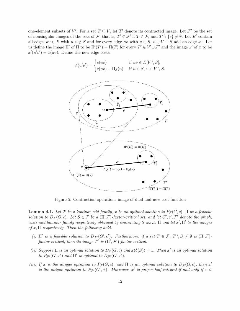
one-element subsets of V ′. For a set T ⊆ V , let T ′ denote its contracted image. Let F ′ be the setof nonsingular images of the sets of F , that is, T ′ ∈ F ′ if T ∈ F , and T ′ \ s 6= ∅. Let E′ containall edges uv ∈ E with u, v /∈ S and for every edge uv with u ∈ S, v ∈ V − S add an edge sv. Letus define the image Π′ of Π to be Π′(T ′) = Π(T ) for every T ′ ∈ V ′ ∪F ′ and the image x′ of x to bex′(u′v′) = x(uv). Define the new edge costs

c′(u′v′) =

c(uv) if uv ∈ E[V \ S],

c(uv)−ΠS(u) if u ∈ S, v ∈ V \ S.

Figure 5: Contraction operation: image of dual and new cost function

Lemma 4.1. Let F be a laminar odd family, x be an optimal solution to PF (G, c), Π be a feasiblesolution to DF (G, c). Let S ∈ F be a (Π,F)-factor-critical set, and let G′, c′,F ′ denote the graph,costs and laminar family respectively obtained by contracting S w.r.t. Π and let x′,Π′ be the imagesof x,Π respectively. Then the following hold.

(i) Π′ is a feasible solution to DF ′(G′, c′). Furthermore, if a set T ∈ F , T \ S 6= ∅ is (Π,F)-

factor-critical, then its image T ′ is (Π′,F ′)-factor-critical.

(ii) Suppose Π is an optimal solution to DF (G, c) and x(δ(S)) = 1. Then x′ is an optimal solutionto PF ′(G

′, c′) and Π′ is optimal to DF ′(G′, c′).

(iii) If x is the unique optimum to PF (G, c), and Π is an optimal solution to DF (G, c), then x′

is the unique optimum to PF ′(G′, c′). Moreover, x′ is proper-half-integral if and only if x is

12

proper-half-integral. Further, assume C ′ is an odd cycle in supp(x′) and let T be the pre-imageof V (C ′) in G. Then, supp(x) inside T consists of an odd cycle and matching edges.

Proof. (i) For feasibility, it is sufficient to verify∑T ′∈V ′∪F ′:u′v′∈δ(T ′)

Π′(T ′) ≤ c′(u′v′) ∀u′v′ ∈ E′.

If u, v 6= s, this is immediate from feasibility of Π to DFi(G, c). Consider an edge sv′ ∈ E(G′). Letuv be the pre-image of this edge.∑

T ′∈V ′∪F ′:sv′∈δ(T ′)

Π′(T ′) = Π(S) +∑

T∈F :uv∈δ(T ),T\S 6=∅

Π(T ) ≤ c(uv)−ΠS(u) = c′(sv′).

We also observe that u′v′ is tight in G′ w.r.t Π′ if and only if the pre-image uv is tight in G w.r.tΠ.

Let T ∈ F be (Π,F)-factor-critical with T \ S 6= ∅. It is sufficient to verify that T ′ is (Π′,F ′)-factor-critical whenever T contains S. Let u′ ∈ T ′ be the image of u ∈ V , and consider theprojection M ′ of the Π-critical-matching Mu. The support of this projection is contained in thetight edges with respect to Π′. Let Z ′ ( T ′, Z ′ ∈ F ′ and let Z be the pre-image of Z ′. If u′ 6= s,then |M ′ ∩ δ(Z ′)| = |Mu ∩ δ(Z)| ≤ 1 and since |Mu ∩ δ(S)| = 1 by Lemma 2.2, the matchingM ′ is a (T ′ \ u′,F ′)-perfect-matching. If u′ = s, then u ∈ S. By Lemma 2.2, Mu ∩ δ(S) = ∅and hence, M ′ misses s. Also, |Mu ∩ δ(Z)| ≤ 1 implies |M ′ ∩ δ(Z ′)| ≤ 1 and hence M ′ is a(T ′ \ s,F ′)-perfect-matching.

(ii) Since x(δ(S)) = 1, we have x′(δ(v)) = 1 for every v ∈ V ′. It is straightforward to verifythat x′(δ(T ′)) ≥ 1 for every T ′ ∈ F ′ with equality if x(δ(T )) = 1. Thus, x′ is feasible to PF ′(G

′, c′).Optimality follows as x′ and Π′ satisfy complementary slackness, using that the image of tightedges is tight, as shown by the argument for part (i).

(iii) For uniqueness, consider an arbitrary optimal solution y′ to PF ′(G′, c′). Let Mu be the

Π-critical matching for u in S. Define αu = y′(δ(u)) for every u ∈ S, i.e., αu is the total y′ valueon the images of edges uv ∈ E with v ∈ V − S. Note that

∑u∈S αu = y′(δ(S)) = 1. Take

w =∑

u∈S αuMu and

y(uv) =

y′(u′v′) if uv ∈ E \ E[S],

w(uv) if uv ∈ E[S].

Then, y is a feasible solution to PF (G, c) and y satisfies complementary slackness with Π. Hence,y is an optimum to PF (G, c) and thus by uniqueness, we get y = x. Consequently, y′ = x′.

The above argument also shows that x must be identical to w inside S. Suppose x′ is proper-half-integral. First, assume s is covered by a matching edge in x′. Then αu = 1 for some u ∈ Sand αv = 0 for every v 6= u. Consequently, w = Mu is a perfect matching on S − u. Next,assume s is incident to an odd cycle in x′. Then αu1 = αu2 = 1/2 for some nodes u1, u2 ∈ S, andw = 1

2(Mu1 + Mu2). The uniqueness of x implies the uniqueness of both Mu1 and Mu2 . Then byLemma 2.2(ii), the symmetric difference of Mu1 and Mu2 may not contain any even cycles. Hence,supp(w) contains an even path between u1 and u2, and some matching edges. Consequently, x isproper-half-integral. The above argument immediately shows the following.

Claim 4.2. Let C ′ be an odd (even) cycle such that x′(e) = 1/2 for every e ∈ C ′ in supp(x′) andlet T be the pre-image of the set V (C ′) in G. Then, supp(x)∩E[T ] consists of an odd (even) cycleC and a (possibly empty) set M of edges such that x(e) = 1/2 ∀ e ∈ C and x(e) = 1 ∀ e ∈M .

13

Next, we prove that if x is proper-half-integral, then so is x′. It is clear that x′ being the imageof x is half-integral. If x′ is not proper-half-integral, then supp(x′) contains an even 1/2-cycle, andthus by Claim 4.2, supp(x) must also contain an even cycle, contradicting that it was proper-half-integral. Finally, if C ′ is an odd cycle in supp(x′), then Claim 4.2 provides the required structurefor x inside T . We also need to show that its support does not contain an even cycle C ′. If not,then the same argument as above shows that the pre-image of C ′ is an even cycle C in the supportof x, a contradiction.

Corollary 4.3. Assume x is the optimal solution to PF (G, c) and there exists an F-positively-criticaldual optimum Π. Let G, c be the graph, and cost obtained by contracting all maximal sets S ∈ Fwith Π(S) > 0 w.r.t. Π, and let x be the image of x in G.

(i) x and Π are the optimal solutions to the bipartite relaxation P0(G, c) and D0(G, c) respectively.

(ii) If x is the unique optimum to PF (G, c), then x is the unique optimum to P0(G, c). If x isproper-half-integral, then x is also proper-half-integral.

Proof of Lemma 3.1. Let Π be an F-positively-critical dual optimum, and let x be the uniqueoptimal solution to PF (G, c). Contract all maximal sets S ∈ F with Π(S) > 0, obtaining thegraph G and cost c. Let x be the image of x in G. By Corollary 4.3(ii), x is unique optimumto P0(G, c). By Proposition 1.2, x is proper-half-integral and hence by Corollary 4.3(ii), x is alsoproper-half-integral.

5 Structure of dual solutions

In this section, we show two properties about positively-critical dual optimal solutions – (1) anoptimum Ψ to DF (G, c) can be transformed into an F-positively-critical dual optimum (Section5.2) if F is a critical family and (2) a Γ-extremal dual optimal solution to DF (G, c) as obtained inthe algorithm is also an F-positively-critical dual optimal solution (Section 5.3). In Section 5.1, wefirst show some lemmas characterizing arbitrary dual optimal solutions.

5.1 Consistency of dual solutions

Assume F ⊆ O is a critical family, with Π being an F-critical dual solution, and let Ψ be anarbitrary dual optimal solution to DF (G, c). Note that optimality of Π is not assumed. Let x bean optimal solution to PF (G, c); we do not assume uniqueness in this section. We shall describestructural properties of Ψ compared to Π; in particular, we show that if we contract a Π-factor-critical set S, the images of x and Ψ will be primal and dual optimal solutions in the contractedgraph.

Consider a set S ∈ F . We say that the dual solutions Π and Ψ are identical inside S, ifΠ(T ) = Ψ(T ) for every set T ( S, T ∈ F ∪ V. We defined ΠS(u) in the previous section; we alsouse this notation for Ψ, namely, let ΨS(u) :=

∑T∈V∪F :T(S,u∈T Ψ(T ) for u ∈ S. Let us now define

∆Π,Ψ(S) := maxu∈S

(ΠS(u)−ΨS(u)) .

We say that Ψ is consistent with Π inside S, if ΠS(u)−ΨS(u) = ∆Π,Ψ(S) holds for every u ∈ S thatis incident to an edge uv ∈ δ(S) ∩ supp(x). The main goal of this section is to prove the followinglemma.

14

Lemma 5.1. Let F ⊆ O be a critical family, with Π being an F-critical dual solution and let Ψ bean optimal solution to DF (G, c). Let x be an optimal solution to PF (G, c). Then Ψ is consistentwith Π inside every set S ∈ F such that x(δ(S)) = 1. Further, ∆Π,Ψ(S) ≥ 0 for all such sets.

Consistency is important as it enables us to preserve optimality when contracting a set S ∈ Fw.r.t. Π. Assume Ψ is consistent with Π inside S, and x(δ(S)) = 1. Let us contract S w.r.t. Π toobtain G′ and c′ as defined in Section 4. Define

Ψ′(T ′) =

Ψ(T ) if T ′ ∈ (F ′ ∪ V ′) \ s,Ψ(S)−∆Π,Ψ(S) if T ′ = s

Lemma 5.2. Let F ⊆ O be a critical family, with Π being an F-critical dual solution and let Ψ bean optimal solution to DF (G, c). Let x be an optimal solution to PF (G, c). Suppose Ψ is consistentwith Π inside S ∈ F and x(δ(S)) = 1. Let G′, c′,F ′ denote the graph, costs and laminar familyobtained by contraction. Then the image x′ of x is an optimum to PF ′(G

′, c′), and Ψ′ (as definedabove) is an optimum to DF ′(G

′, c′).

Proof. Feasibility of x′ follows as in the proof of Lemma 4.1(ii). For the feasibility of Ψ′, we haveto verify

∑T ′∈V ′∪F ′:uv∈δ(T ′) Ψ′(T ′) ≤ c′(uv) for every edge uv ∈ E(G′). This follows immediately

for every edge uv such that u, v 6= s since Ψ is a feasible solution for DF (G, c). Consider an edgeuv ∈ E(G), u ∈ S. Let sv ∈ E(G′) be the image of uv in G′, and let ∆ = ∆Π,Ψ(S).

c(uv) ≥∑

T∈V∪F :uv∈δ(T )

Ψ(T )

= ΨS(u) + Ψ(S) +∑

T∈F :uv∈δ(T ),T−S 6=∅

Ψ(T )

= ΨS(u) + ∆ +∑

T ′∈V ′∪F ′:sv∈δ(T ′)

Ψ′(T ′).

In the last equality, we used the definition Ψ′(s) = Ψ(S)−∆. Therefore, using ΠS(u) ≤ ΨS(u)+∆,we obtain ∑

T ′∈V ′∪F ′:sv∈δ(T ′)

Ψ′(T ′) ≤ c(uv)−ΨS(u)−∆ ≤ c(uv)−ΠS(u) = c′(uv). (1)

Thus, Ψ′ is a feasible solution to DF ′(G′, c′). To show optimality, we verify complementary slackness

for x′ and Ψ′. If x′(uv) > 0 for u, v 6= s, then x(uv) > 0. Thus, the tightness of the constraintfor uv w.r.t. Ψ′ in DF ′(G

′, c′) follows from the tightness of the constraint w.r.t. Ψ in DF (G, c).Suppose x′(sv) > 0 for an edge sv ∈ E(G′). Let uv ∈ E(G) be the pre-image of sv for some u ∈ S.Then the tightness of the constraint follows since both the inequalities in (1) are tight – the firstinequality is tight since uv is tight w.r.t. Ψ, and the second is tight since ΠS(u) − ΨS(u) = ∆(S)by the consistency property. Finally, if Ψ′(T ′) > 0 for some T ′ ∈ F ′, then Ψ(T ) > 0 and hencex(δ(T )) = 1 and therefore, x′(δ(T ′)) = 1.

Lemma 5.3. Let F be a critical family with Π being an F-critical dual, and let x be an optimalsolution to PF (G, c). If x(δ(S)) = 1 for some S ∈ F , then all edges in supp(x) ∩ E[S] are tightw.r.t. Π and x(δ(T )) = 1 for every T ( S, T ∈ F .

Proof. Let αu = x(δ(u, V \ S)) for each u ∈ S, and for each T ⊆ S, T ∈ F , let α(T ) =∑

u∈T αu =x(δ(T, V \S)). Note that α(S) = x(δ(S)) = 1. Let us consider the following pair of linear programs.

15

min∑

uv∈E[S]

c(uv)z(uv) (PF [S])

z(δ(u)) = 1− αu ∀u ∈ Sz(δ(T )) ≥ 1− α(T ) ∀T ( S, T ∈ Fz(uv) ≥ 0 ∀ uv ∈ E[S]

max∑

T(S,T∈V∪F(1− α(T ))Γ(T ) (DF [S])

∑T(S,T∈V∪Fuv∈δ(T )

Γ(T ) ≤ c(uv) ∀uv ∈ E[S]

Γ(Z) ≥ 0 ∀Z ( T,Z ∈ F

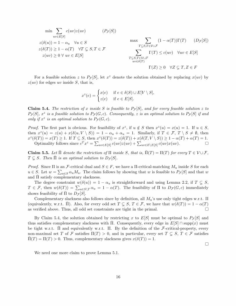
For a feasible solution z to PF [S], let xz denote the solution obtained by replacing x(uv) byz(uv) for edges uv inside S, that is,

xz(e) =

x(e) if e ∈ δ(S) ∪ E[V \ S],

z(e) if e ∈ E[S].

Claim 5.4. The restriction of x inside S is feasible to PF [S], and for every feasible solution z toPF [S], xz is a feasible solution to PF (G, c). Consequently, z is an optimal solution to PF [S] if andonly if xz is an optimal solution to PF (G, c).

Proof. The first part is obvious. For feasibility of xz, if u /∈ S then xz(u) = x(u) = 1. If u ∈ S,then xz(u) = z(u) + x(δ(u, V \ S)) = 1 − αu + αu = 1. Similarly, if T ∈ F , T \ S 6= ∅, thenxz(δ(T )) = x(T ) ≥ 1. If T ⊆ S, then xz(δ(T )) = z(δ(T )) + x(δ(T, V \ S)) ≥ 1− α(T ) + α(T ) = 1.

Optimality follows since cTxz =∑

uv∈E[S] c(uv)z(uv) +∑

uv∈E\E[S] c(uv)x(uv).

Claim 5.5. Let Π denote the restriction of Π inside S, that is, Π(T ) = Π(T ) for every T ∈ V ∪F ,T ( S. Then Π is an optimal solution to DF [S].

Proof. Since Π is an F-critical dual and S ∈ F , we have a Π-critical-matching Mu inside S for eachu ∈ S. Let w =

∑u∈S αuMu. The claim follows by showing that w is feasible to PF [S] and that w

and Π satisfy complementary slackness.The degree constraint w(δ(u)) = 1 − αu is straightforward and using Lemma 2.2, if T ( S,

T ∈ F , then w(δ(T )) =∑

u∈S\T αu = 1 − α(T ). The feasibility of Π to DF (G, c) immediately

shows feasibility of Π to DF [S].Complementary slackness also follows since by definition, all Mu’s use only tight edges w.r.t. Π

(equivalently, w.r.t. Π). Also, for every odd set T ( S, T ∈ F , we have that w(δ(T )) = 1 − α(T )as verified above. Thus, all odd set constraints are tight in the primal.

By Claim 5.4, the solution obtained by restricting x to E[S] must be optimal to PF [S] andthus satisfies complementary slackness with Π. Consequently, every edge in E[S] ∩ supp(x) mustbe tight w.r.t. Π and equivalently w.r.t. Π. By the definition of the F-critical-property, everynon-maximal set T of F satisfies Π(T ) > 0, and in particular, every set T ( S, T ∈ F satisfiesΠ(T ) = Π(T ) > 0. Thus, complementary slackness gives x(δ(T )) = 1.

We need one more claim to prove Lemma 5.1.

16

Claim 5.6. Let S ∈ F be an inclusionwise minimal set of F . Let Λ and Γ be feasible solutionsto DF (G, c), and suppose S is (Λ,F)-factor-critical. Then ∆Λ,Γ(S) = maxu∈S |ΛS(u) − ΓS(u)|.Further, if ∆Λ,Γ(S) > 0, define

A+ := u ∈ S : Γ(u) = Λ(u) + ∆Λ,Γ(S),A− := u ∈ S : Γ(u) = Λ(u)−∆Λ,Γ(S).

Then |A−| > |A+|.

Proof. Let ∆ = maxu∈S |ΛS(u)−ΓS(u)|, and define the sets A− and A+ with ∆ instead of ∆Λ,Γ(S).Since S is (Λ,F)-factor-critical, for every a ∈ S, there exists an (S \ a,F) perfect matching Ma

using only tight edges w.r.t. Λ, i.e., Ma ⊆ uv : Λ(u) + Λ(v) = c(uv) by the minimality of S.Further, by feasibility of Γ, we have Γ(u) + Γ(v) ≤ c(uv) on every uv ∈ Ma. Thus, if u ∈ A+,then v ∈ A− for every uv ∈ Ma. Since ∆ > 0, we have A+ ∪ A− 6= ∅ and therefore A− 6= ∅,and consequently, ∆ = ∆Λ,Γ(S). Now pick a ∈ A− and consider Ma. This perfect matching Ma

matches each node in A+ to a node in A−. Thus, |A−| > |A+|.

Proof of Lemma 5.1. We prove this by induction on |V |, and subject to this, on |S|. Since Π is anF-critical dual solution, each set S ∈ F is (Π,F)-factor-critical. First, consider the case when S isan inclusion-wise minimal set. Then, ΠS(u) = Π(u), ΨS(u) = Ψ(u) for every u ∈ S. By Claim 5.6,we have that ∆ := ∆Π,Ψ(S) ≥ 0. We are done if ∆ = 0. Otherwise, define the sets A− and A+ asin the claim using ∆Π,Ψ(S).

Now consider an edge uv ∈ E[S]∩supp(x). By complementary slackness, we have Ψ(u)+Ψ(v) =c(uv). By dual feasibility, we have Π(u) + Π(v) ≤ c(uv). Hence, if u ∈ A−, then v ∈ A+.Consequently, we have

|A−| =∑u∈A−

x(δ(u)) = x(δ(A−, V \ S)) + x(δ(A−, A+))

≤ 1 +∑u∈A+

x(δ(u)) = 1 + |A+| ≤ |A−|.

Thus, we should have equality throughout. Hence, x(δ(A−, V \ S)) = 1. This precisely means thatΨ is consistent with Π inside S.

Next, let S be a non-minimal set. Let T ∈ F be a maximal set strictly contained in S. ByLemma 5.3, x(δ(T )) = 1, therefore the inductional claim holds for T : Ψ is consistent with Π insideT , and ∆(T ) = ∆Π,Ψ(T ) ≥ 0.

We contract T w.r.t. Π and use Lemma 5.2. Let the image of the solutions x, Π, and Ψ be x′, Π′

and Ψ′ respectively and the resulting graph be G′ with cost function c′. Then x′ and Ψ′ are optimumto PF ′(G

′, c′) and DF ′(G′, c′) respectively, and by Lemma 4.1(i), Π′ is an F ′-critical dual. Let t be

the image of T by the contraction. Now, consider the image S′ of S in G′. Since G′ is a smallergraph, it satisfies the induction hypothesis. Let ∆′ = ∆Π′,Ψ′(S

′) in G′. By induction hypothesis,∆′ ≥ 0. The following claim verifies consistency inside S and thus completes the proof.

Claim 5.7. For every u ∈ S, ΠS(u)−ΨS(u) ≤ Π′S′(u′)−Ψ′S′(u

′), and equality holds if there existsan edge uv ∈ δ(S) ∩ supp(x). Consequently, ∆′ = ∆.

17

Proof. Let u′ denote the image of u. If u′ 6= t, then Π′S′(u′) = ΠS(u),Ψ′S′(u

′) = ΨS(u) and therefore,ΠS(u)−ΨS(u) = Π′S′(u

′)−Ψ′S′(u′). Assume u′ = t, that is, u ∈ T . Then ΠS(u) = ΠT (u) + Π(T ),

ΨS(u) = ΨT (u) + Ψ(T ) by the maximal choice of T , and therefore

ΠS(u)−ΨS(u) = ΠT (u)−ΨT (u) + Π(T )−Ψ(T )

≤ ∆(T ) + Π(T )−Ψ(T )

= Π′(t)−Ψ′(t) (Since Π′(t) = Π(T ), Ψ′(t) = Ψ(T )−∆(T ))

= Π′S′(t)−Ψ′S′(t). (2)

Assume now that there exists a uv ∈ δ(S)∩ supp(x). If u ∈ T , then using the consistency inside T ,we get ΠT (u)−ΨT (u) = ∆(T ), and therefore (2) gives ΠS(u)−ΨS(u) = Π′S′(t)−Ψ′S′(t) = ∆′.

Claim 5.6 can also be used to derive the following important property.

Lemma 5.8. Given a laminar odd family F ⊂ O, let Λ and Γ be two dual feasible solutions toDF (G, c). If a subset S ∈ F is both (Λ,F)-factor-critical and (Γ,F)-factor-critical, then Λ and Γare identical inside S.

Proof. Consider a graph G = (V,E) with |V | minimal, where the claim does not hold for someset S. Also, choose S to be the smallest counterexample in this graph. First, assume S ∈ F is aminimal set. Then consider Claim 5.6 for Λ and Γ and also by changing their roles, for Γ and Λ.If Λ and Γ are not identical inside S, then ∆ = maxu∈S |ΛS(u)− ΓS(u)| > 0. The sets A− and A+

for Λ and Γ become A+ and A− for Γ and Λ. Then |A−| > |A+| > |A−|, a contradiction.Suppose now S contains T ∈ F . It is straightforward to see that T is also (Λ,F)-factor-critical

and (Γ,F)-factor-critical by definition. Thus, by the minimal choice of the counterexample S, wehave that Λ and Γ are identical inside T . Now, contract the set T w.r.t. Λ, or equivalently, w.r.t.Γ. Let Λ′, Γ′ denote the contracted solutions in G′, and let F ′ be the contraction of F . Then, byLemma 4.1(i), these two solutions are feasible to DF ′(G

′, c′), and S′ is both Λ′-factor-critical andΓ′-factor-critical. Now, Λ′ and Γ′ are not identical inside S′, contradicting the minimal choice of Gand S.

5.2 Finding a positively-critical dual optimal solution

Let F ⊆ O be a critical family with Π being an F-critical dual. Let Ψ be a dual optimum solutionto DF (G, c). Our goal is to satisfy the property that for every S ∈ F , if Ψ(S) > 0, then Ψ and Πare identical inside S. By Lemma 5.8, it is equivalent to showing that Ψ is F-positively-critical.We modify Ψ by the algorithm shown in Figure 6.

The correctness of the algorithm follows by showing that the modified solution Ψ is also dualoptimal, and it is closer to Π.

Lemma 5.9. Let F ⊆ O be a critical family with Π being an F-critical dual and let Ψ be a dualoptimum solution to DF (G, c). Suppose we consider a maximal set S such that Π and Ψ are notidentical inside S, take λ = min1,Ψ(S)/∆Π,Ψ(S) if ∆Π,Ψ(S) > 0 and λ = 1 if ∆Π,Ψ(S) = 0 andset Ψ as in (3). Then, Ψ is also a dual optimal solution to DF (G, c), and either Ψ(S) = 0 or Πand Ψ are identical inside S.

Proof. Let x be an optimal solution to PF (G, c). Since Ψ(S) > 0, we have x(δ(S)) = 1 and byLemma 5.1, we have ∆ = ∆Π,Ψ(S) ≥ 0. Now, the second conclusion is immediate from definition:

18

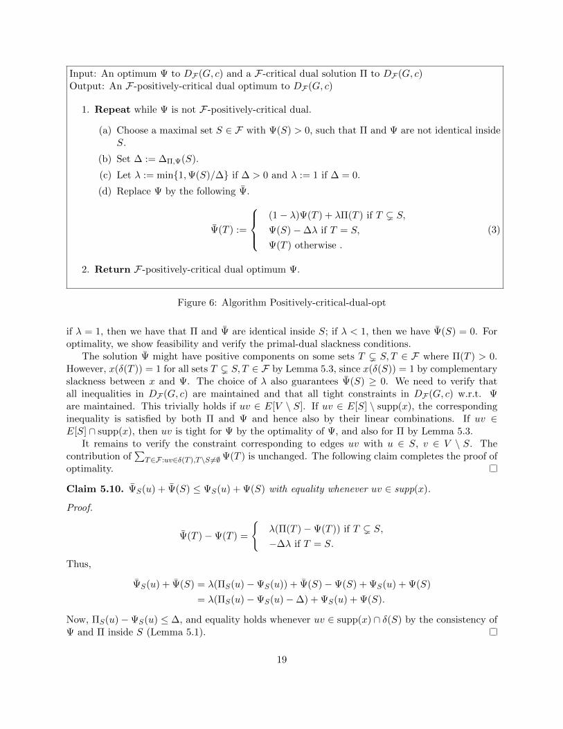
Input: An optimum Ψ to DF (G, c) and a F-critical dual solution Π to DF (G, c)Output: An F-positively-critical dual optimum to DF (G, c)

1. Repeat while Ψ is not F-positively-critical dual.

(a) Choose a maximal set S ∈ F with Ψ(S) > 0, such that Π and Ψ are not identical insideS.

(b) Set ∆ := ∆Π,Ψ(S).

(c) Let λ := min1,Ψ(S)/∆ if ∆ > 0 and λ := 1 if ∆ = 0.

(d) Replace Ψ by the following Ψ.

Ψ(T ) :=

(1− λ)Ψ(T ) + λΠ(T ) if T ( S,

Ψ(S)−∆λ if T = S,

Ψ(T ) otherwise .

(3)

2. Return F-positively-critical dual optimum Ψ.

Figure 6: Algorithm Positively-critical-dual-opt

if λ = 1, then we have that Π and Ψ are identical inside S; if λ < 1, then we have Ψ(S) = 0. Foroptimality, we show feasibility and verify the primal-dual slackness conditions.

The solution Ψ might have positive components on some sets T ( S, T ∈ F where Π(T ) > 0.However, x(δ(T )) = 1 for all sets T ( S, T ∈ F by Lemma 5.3, since x(δ(S)) = 1 by complementaryslackness between x and Ψ. The choice of λ also guarantees Ψ(S) ≥ 0. We need to verify thatall inequalities in DF (G, c) are maintained and that all tight constraints in DF (G, c) w.r.t. Ψare maintained. This trivially holds if uv ∈ E[V \ S]. If uv ∈ E[S] \ supp(x), the correspondinginequality is satisfied by both Π and Ψ and hence also by their linear combinations. If uv ∈E[S] ∩ supp(x), then uv is tight for Ψ by the optimality of Ψ, and also for Π by Lemma 5.3.

It remains to verify the constraint corresponding to edges uv with u ∈ S, v ∈ V \ S. Thecontribution of

∑T∈F :uv∈δ(T ),T\S 6=∅Ψ(T ) is unchanged. The following claim completes the proof of

optimality.

Claim 5.10. ΨS(u) + Ψ(S) ≤ ΨS(u) + Ψ(S) with equality whenever uv ∈ supp(x).

Proof.

Ψ(T )−Ψ(T ) =

λ(Π(T )−Ψ(T )) if T ( S,

−∆λ if T = S.

Thus,

ΨS(u) + Ψ(S) = λ(ΠS(u)−ΨS(u)) + Ψ(S)−Ψ(S) + ΨS(u) + Ψ(S)

= λ(ΠS(u)−ΨS(u)−∆) + ΨS(u) + Ψ(S).

Now, ΠS(u)−ΨS(u) ≤ ∆, and equality holds whenever uv ∈ supp(x) ∩ δ(S) by the consistency ofΨ and Π inside S (Lemma 5.1).

19

Corollary 5.11. Let F be a critical family with Π being an F-critical dual feasible solution. Al-gorithm Positively-critical-dual-opt in Figure 6 transforms an arbitrary dual optimal solution Ψ toan F-positively-critical dual optimal solution in at most |F| iterations.

Proof. The correctness of the algorithm follows by Lemma 5.9. We bound the running time byshowing that no set S ∈ F is processed twice. After a set S is processed, by Lemma 5.9, eitherΠ and Ψ will be identical inside S or Ψ(S) = 0. Once Π and Ψ become identical inside a set, itremains so during all later iterations.

The value Ψ(S) could be changed later only if we process a set S′ ) S after processing S. Let S′

be the first such set. At the iteration when S was processed, by the maximal choice it follows thatΨ(S′) = 0. Hence Ψ(S′) could become positive only if the algorithm had processed a set Z ) S′,Z ∈ F between processing S and S′, a contradiction to the choice of S′.

5.3 Extremal dual solutions

In this section, we prove Lemma 3.2. Assume F ⊆ O is a critical family, with Π being an F-criticaldual. Let x be the unique optimal solution to PF (G, c). Let Fx = S ∈ F : x(δ(S)) = 1 thecollection of tight sets for x. A Π-extremal dual can be found by solving the following LP.

minh(Ψ,Π) =∑

S∈V∪Fx

r(S)

|S|(D∗F )

−r(S) ≤ Ψ(S)−Π(S) ≤ r(S) ∀S ∈ V ∪ Fx∑S∈V∪Fx:uv∈δ(S)

Ψ(S) = c(uv) ∀uv ∈ supp(x)

∑S∈V∪Fx:uv∈δ(S)

Ψ(S) ≤ c(uv) ∀uv ∈ E \ supp(x)

Ψ(S) ≥ 0 ∀S ∈ Fx

The support of Ψ is restricted to sets in V ∪ Fx. Primal-dual slackness implies that the feasiblesolutions to this program coincide with the optimal solutions of DF (G, c), hence an optimal solutionto D∗F is also an optimal solution to DF (G, c).

Lemma 5.12. Let F ⊂ O be a critical family with Π being an F-critical dual. Then, a Π-extremaldual is also an F-positively-critical dual optimal solution.

Proof. We will show that whenever Ψ(S) > 0, the solutions Ψ and Π are identical inside S.Assume for a contradiction that this is not true for some S ∈ F . Let λ = min1,Ψ(S)/∆Π,Ψ(S)if ∆Π,Ψ(S) > 0 and λ = 1 if ∆Π,Ψ(S) = 0. Define Ψ as in (3). By Lemma 5.9, Ψ is also optimal toDF (G, c) and thus feasible to D∗F . We show h(Ψ,Π) < h(Ψ,Π), which is a contradiction.

For every T ∈ V ∪ Fx, let τ(T ) = |Ψ(T )−Π(T )| − |Ψ(T )−Π(T )|. With this notation,

h(Ψ,Π)− h(Ψ,Π) =∑

T∈V∪Fx

τ(T )

|T |.

If T \ S = ∅, then Ψ(T ) = Ψ(T ) and thus τ(T ) = 0. If T ( S, T ∈ V ∪ F , then |Ψ(T ) − Π(T )| =(1 − λ)|Ψ(T ) − Π(T )|, and thus τ(T ) = λ|Ψ(T ) − Π(T )|. Since Ψ(S) = Ψ(S) − ∆λ, we haveτ(S) ≥ −∆λ.

20

Let us fix an arbitrary u ∈ S, and let γ = maxT(S:u∈T,T∈V∪Fx |T |.

h(Ψ,Π)− h(Ψ,Π) =∑

T∈V∪Fx

τ(T )

|T |

≥∑

T(S:u∈T,T∈V∪Fx

τ(T )

|T |+τ(S)

|S|

≥ λ

γ

∑T(S:u∈T,T∈V∪Fx

|Ψ(T )−Π(T )| − ∆λ

|S|

≥ λ

γ(ΠS(u)−ΨS(u))− ∆λ

|S|.

Case 1: If ∆ > 0, then pick u ∈ S satisfying ΠS(u)−ΨS(u) = ∆. Then the above inequalities give

h(Ψ,Π)− h(Ψ,Π) ≥ ∆λ

(1

γ− 1

|S|

)> 0.

The last inequality follows since |S| > γ.Case 2: If ∆ = 0, then λ = 1 and therefore,

h(Ψ,Π)− h(Ψ,Π) ≥ 1

γ

∑T(S:u∈T,T∈V∪Fx

|Ψ(T )−Π(T )|

Now, if Π and Ψ are not identical inside S, then there exists a node u ∈ S for which the RHS isstrictly positive. Thus, in both cases, we get h(Ψ,Π) < h(Ψ,Π), a contradiction to the optimalityof Ψ to D∗F .

Proof of Lemma 3.2. By Lemma 3.1, the unique optimal x to PF (G, c) is proper-half-integral.Lemma 5.12 already shows that a Γ-extremal dual solution Π is also F-positively-critical. Weneed to show that the next family of cuts is a critical family. Recall that the set of cuts for thenext round is defined as H′ ∪ H′′, where H′ = T ∈ F : Π(T ) > 0, and H′′ is defined based onsome cycles in supp(x). We need to show that every set of H′ ∪ H′′ is Π-factor-critical. This isstraightforward for sets of H′ by the definition of the F-positively-critical property.

It remains to show that the sets of H′′ are also Π-factor-critical. These are defined for oddcycles C ∈ supp(x). Now, C ∈ H′′ is the union of V (C) and the maximal sets S1, . . . , S` of H′intersecting V (C). We have Π(Sj) > 0 for each j = 1, . . . , ` and hence x(δ(Sj)) = 1.

Let u ∈ C be an arbitrary node; we will construct the Π-critical matching Mu. Let us contractall sets S1, . . . , S` to nodes s1, . . . , s` w.r.t. Π. We know by Lemma 4.1(iii) that the image x′ ofx is proper-half-integral and that the cycle C projects to a cycle in x′. The proper-half-integralproperty guarantees that C is contracted into an odd cycle C ′ in supp(x′). Let u′ be the image ofu; the pre-image of every edge in C ′ is a tight edge w.r.t. Π in the original graph since Π is anoptimum to the dual problem DF (G, c). Since C ′ is an odd cycle, there is a perfect matching M ′u′that covers every node in V (C ′) \ u′ using the edges in C ′.

Assume first u ∈ Sj for some 1 ≤ j ≤ `. Then u′ = sj . The pre-image M of M ′u′ in the originalgraph contains exactly one edge entering each Sk for k 6= j and no edges entering Sj . Consider theΠ-critical matching Mu for u in Sj . For k 6= j, if akbk ∈ M ∩ δ(Sk), ak ∈ Sk, then, let Mak be the

21

Π-critical matching for ak in Sk. The union of M , Mu and the Mak ’s give a Π-critical matching foru inside C.

If u ∈ C \ (∪`j=1Sj), then similarly there is a Π-critical matching Mak inside every Sk. The

union of M and the Mak ’s give the Π-critical matching for u inside C. We also have Π(S) > 0 forall non-maximal sets S ∈ H′ ∪H′′ since the only sets with Π(S) = 0 are those in H′′, and they areall maximal ones.

6 Convergence

The goal of this section is to prove Lemmas 3.3 and 3.4. The first shows that the number ofodd cycles in the support is nonincreasing, and the second shows that in a sequence of iterationswhere the number of cycles does not decrease, all the new cuts added continue to be includedin subsequent iterations (till the number of cycles decreases). These structural properties areestablished as follows. First, we give an extension of Edmonds’ primal-dual algorithm to half-integral matchings. Next, we argue that applying this algorithm to the current primal/dual solutionleads to an optimal solution of the next LP. The analysis of the algorithm shows that the numberof odd cycles is nonincreasing. Finally, we prove the extremal dual solution of the next LP mustbe the same as the one found by this combinatorial algorithm, and therefore the LP solution weuse also satisfies the required properties.

As mentioned in the introduction, our extension of Edmonds’ algorithm to the half-integralsetting and its application are for the purpose of analysis. We describe this algorithm first, deriveits properties, then use it in the main proof of convergence of the cutting plane algorithm.

6.1 The half-integral matching algorithm

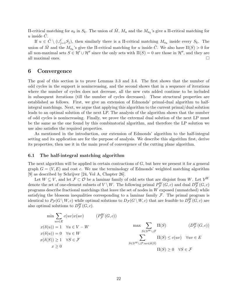
The next algorithm will be applied in certain contractions of G, but here we present it for a generalgraph G = (V,E) and cost c. We use the terminology of Edmonds’ weighted matching algorithm[9] as described by Schrijver [24, Vol A, Chapter 26].

Let W ⊆ V , and let F ⊂ O be a laminar family of odd sets that are disjoint from W . Let VWdenote the set of one-element subsets of V \W . The following primal PWF (G, c) and dual DW

F (G, c)programs describe fractional matchings that leave the set of nodes in W exposed (unmatched) whilesatisfying the blossom inequalities corresponding to a laminar family F . The primal program isidentical to PF (G \W, c) while optimal solutions to DF (G \W, c) that are feasible to DW

F (G, c) arealso optimal solutions to DW

F (G, c).

min∑uv∈E

c(uv)x(uv) (PWF (G, c))

x(δ(u)) = 1 ∀u ∈ V −Wx(δ(u)) = 0 ∀u ∈Wx(δ(S)) ≥ 1 ∀S ∈ F

x ≥ 0

max∑

S∈VW∪F

Π(S) (DWF (G, c))

∑S∈VW∪F :uv∈δ(S)

Π(S) ≤ c(uv) ∀uv ∈ E

Π(S) ≥ 0 ∀S ∈ F

22

The algorithm is iterative. In each iteration, it maintains a set T ⊆W , a subset L ⊆ F of cuts,a proper-half-integral optimal solution z to P TL (G, c), and an L-critical dual optimal solution Λ toDTL(G, c) such that Λ(S) > 0 for every S ∈ L. In the beginning T = W , L = F and the algorithm

terminates when T = ∅.We work on the graph G∗ = (V∗, E∗), obtained the following way from G: We first remove

every edge in E that is not tight w.r.t. Λ, and then contract all maximal sets of L w.r.t. Λ. Thenode set of V∗ is identified with the pre-images. Let c∗ denote the contracted cost function and z∗

the image of z. Since E∗ consists only of tight edges, Λ(u) + Λ(v) = c∗(uv) for every edge uv ∈ E∗.Since F is disjoint from W , the nodes in L will always have degree 1 in z∗.

In the course of the algorithm, we may decrease Λ(S) to 0 for a maximal set S of L. In thiscase, we remove S from L and modify G∗, c∗ and z∗ accordingly. This operation will be referredas ‘unshrinking’ S. New sets will never be added to L.

The algorithm works by modifying the solution z∗ and the dual solution Λ∗. An edge uv ∈ E∗ iscalled a 0-edge/1

2 -edge/1-edge according to the value z∗(uv). A modification of z∗ in G∗ naturallyextends to a modification of z in G. Indeed, if S ∈ L∗ is a shrunk node, and z∗ is modified sothat there is an 1-edge incident to S in G∗, then let u1v1 be the pre-image of this edge in G, withu1 ∈ S. Then modify z inside S to be identical with the Λ-critical-matching Mu1 inside S. If thereare two half-edges incident to S in G∗, then let u1v1, u2v2 be the pre-image of these edges in G, withu1, u2 ∈ S. Then modify z inside S to be identical with the convex combination (1/2)(Mu1 +Mu2)of the Λ-critical-matchings Mu1 and Mu2 inside S.

A walk P = v0v1v2 . . . vk in G∗ is called an alternating walk, if every odd edge is a 0-edge andevery even edge is a 1-edge. If every node occurs in P at most once, it is called an alternating path.By alternating along the path P , we mean modifying z∗(vivi+1) to 1− z∗(vivi+1) on every edge ofP . If k is odd, v0 = vk and no other node occurs twice, then P is called a blossom with base v0.The following claim is straightforward.

Claim 6.1 ([24, Thm 24.3]). Let P = v0v1 . . . v2k+1 be an alternating walk. Either P is an alter-nating path, or it contains a blossom C and an even alternating path from v0 to the base of theblossom.

The algorithm is described in Figure 7. The scenarios in Case I are illustrated in Figure 4. InCase II, we observe that T ∈ B+ and further, B+∩B− = ∅ (otherwise, there exists a T−T alternatingwalk and hence we should be in case I). The correctness of the output follows immediately due tocomplementary slackness. We show the termination of the algorithm along very similar lines as theproof of termination of Edmonds’ algorithm.

23

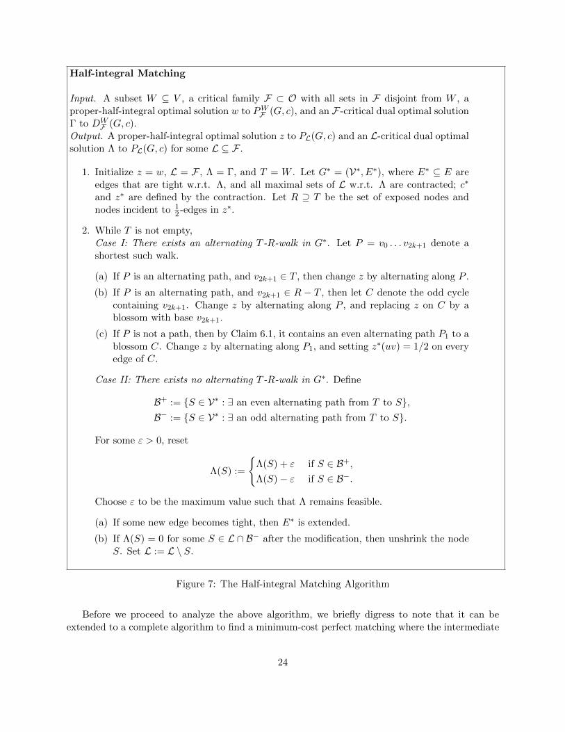
Half-integral Matching

Input. A subset W ⊆ V , a critical family F ⊂ O with all sets in F disjoint from W , aproper-half-integral optimal solution w to PWF (G, c), and an F-critical dual optimal solutionΓ to DW

F (G, c).Output. A proper-half-integral optimal solution z to PL(G, c) and an L-critical dual optimalsolution Λ to PL(G, c) for some L ⊆ F .

1. Initialize z = w, L = F , Λ = Γ, and T = W . Let G∗ = (V∗, E∗), where E∗ ⊆ E areedges that are tight w.r.t. Λ, and all maximal sets of L w.r.t. Λ are contracted; c∗

and z∗ are defined by the contraction. Let R ⊇ T be the set of exposed nodes andnodes incident to 1

2 -edges in z∗.

2. While T is not empty,Case I: There exists an alternating T -R-walk in G∗. Let P = v0 . . . v2k+1 denote ashortest such walk.

(a) If P is an alternating path, and v2k+1 ∈ T , then change z by alternating along P .

(b) If P is an alternating path, and v2k+1 ∈ R − T , then let C denote the odd cyclecontaining v2k+1. Change z by alternating along P , and replacing z on C by ablossom with base v2k+1.

(c) If P is not a path, then by Claim 6.1, it contains an even alternating path P1 to ablossom C. Change z by alternating along P1, and setting z∗(uv) = 1/2 on everyedge of C.

Case II: There exists no alternating T -R-walk in G∗. Define

B+ := S ∈ V∗ : ∃ an even alternating path from T to S,B− := S ∈ V∗ : ∃ an odd alternating path from T to S.

For some ε > 0, reset

Λ(S) :=

Λ(S) + ε if S ∈ B+,

Λ(S)− ε if S ∈ B−.

Choose ε to be the maximum value such that Λ remains feasible.

(a) If some new edge becomes tight, then E∗ is extended.

(b) If Λ(S) = 0 for some S ∈ L ∩ B− after the modification, then unshrink the nodeS. Set L := L \ S.

Figure 7: The Half-integral Matching Algorithm

Before we proceed to analyze the above algorithm, we briefly digress to note that it can beextended to a complete algorithm to find a minimum-cost perfect matching where the intermediate

24

solutions are half-integral and satisfy the degree constraints for all vertices. This complete algorithmand its analysis is presented in the appendix.

Returning to the analysis of the Half-integral Matching algorithm, let β(z) denote the numberof exposed nodes plus the number of cycles in supp(z). We first note that β(z) = β(z∗). Thiscan be derived from Lemma 4.1(iii) (We apply this Lemma in G \ T , observing that P TL (G, c) isidentical to PL(G \T, c)). Our next lemma (Lemma 6.2) shows that β(z) is non-increasing. If β(z)is unchanged during a certain number of iterations of the algorithm, we say that these iterationsform a non-decreasing phase. We say that the algorithm itself is non-decreasing, if β(z) does notdecrease anytime. In the next section, we investigate properties of non-decreasing phases. Theseresults will also show that every non-decreasing phase may contain at most |V |+ |F| iterations andtherefore the algorithm terminates in strongly polynomial time.

Lemma 6.2. Let z be an arbitrary solution during the algorithm, and let α be the number of oddcycles in supp(w) that are absent in supp(z). Then |W | + odd(w) ≥ β(z) + 2α. At termination,|W |+ odd(w) ≥ odd(z) + 2α.

Proof. Initially, β(z) = |W |+odd(w). Let us check the possible changes in β(z) during an iterationof the algorithm. In Case I(a), the number of exposed nodes decreases by two. In Case I(b), boththe number of exposed nodes and the number of cycles decrease by one. In Case I(c), the numberof exposed nodes decreases by one, but we obtain a new odd cycle, hence β(z) remains unchanged.In Case II, z is not modified.

The only way to remove a cycle from supp(z) is by performing the operation in Case I(b).This must be executed α times, therefore β(z) ≤ β(w)− 2α. Further, there are no exposed nodesat the end of the Half-integral Primal-Dual. Thus, on termination β(z) = odd(z), and the claimfollows.

6.1.1 The non-decreasing scenario

Let us now analyze the first non-decreasing phase P of the algorithm, starting from the input w.These results will also be valid for later non-decreasing phases as well. In this case, we say that thealgorithm is non-decreasing. Consider an intermediate iteration with z, Λ being the solutions, Lbeing the laminar family and T being the exposed nodes. Recall that R ⊇ T is the set of exposednodes and the node sets of the 1/2-cycles. Let us define the set of outer/inner nodes of G∗ asthose having even/odd length alternating walk from R in G∗. Let No and Ni denote their sets,respectively. Clearly, B+ ⊆ No, B− ⊆ Ni in Case II of the algorithm.

Lemma 6.3. If P is a non-decreasing phase, then if a node in V∗ is outer in any iteration of phaseP, it remains a node in V∗ and an outer node in every later iteration of P. If a node is innerin any iteration of P, then in any later iteration of P, it is either an inner node, or it has beenunshrunk in an intermediate iteration.

Proof. Since P is a non-decreasing phase, Cases I(a) and (b) can never be performed. We showthat the claimed properties are maintained during an iteration.

In Case I(c), a new odd cycle C is created, and thus C is added to R. Let P1 = v0 . . . v2` denotethe even alternating path with v0 ∈ T , v2` ∈ C. If a node u ∈ V∗ had an even/odd alternatingwalk from v0 before changing the solution, it will have an even/odd walk alternating from v2` ∈ Rafter changing the solution.

25

In Case II, the alternating paths from T to the nodes in B− and B+ are maintained when theduals are changed. The only nontrivial case is when a set S is unshrunk; then all inner and outernodes maintain their inner and outer property by the following: if u1v1 is a 1-edge and u2v2 is a0-edge entering S after unshrinking, with u1, u2 ∈ S, we claim that there exists an even alternatingpath inside S from u1 to u2 using only tight edges wrt Λ. Indeed, during the unshrinking, wemodify z to Mu1 inside S. Also, by the Λ-factor-critical property, all edges of Mu2 are tight w.r.t.Λ. Hence the symmetric difference of Mu1 and Mu2 contains an alternating path from u1 to u2.

We have to check that vertices in No − B+ and Ni − B− also maintain their outer and innerproperty. These are the nodes having even/odd alternating paths from an odd cycle, but not fromexposed nodes. The nodes in these paths are disjoint from B− ∪ B+ and are thus maintained.Indeed, if (B− ∩No) \ B+ 6= ∅ or (B+ ∩Ni) \ B− 6= ∅, then we would get an alternating walk fromT to an odd cycle, giving the forbidden Case I(b).

The termination of the algorithm is guaranteed by the following simple corollary.

Corollary 6.4. The non-decreasing phase P may consist of at most |V |+ |F| iterations.

Proof. Case I may occur at most |W | times as it decreases the number of exposed nodes. In CaseII, either Ni is extended, or a set is unshrunk. By Lemma 6.3, the first scenario may occur at most|V | times and the second at most |F| times.

In the rest of the section, we focus on the case when the entire algorithm is non-decreasing.

Lemma 6.5. Assume the half-integral matching algorithm is non-decreasing. Let Γ be the initialdual and z, Λ be the terminating solution and L be the terminating laminar family. Let No and Nidenote the final sets of outer and inner nodes in G∗.

• If Λ(S) > Γ(S) then S is an outer node in V∗.

• If Λ(S) < Γ(S), then either S ∈ F \ L, (that is, S was unshrunk during the algorithm andΛ(S) = 0) or S is an inner node in V∗, or S is a node in V∗ incident to an odd cycle insupp(z).

Proof. If Λ(S) > Γ(S), then S ∈ B+ in some iteration of the algorithm. By Lemma 6.3, thisremains an outer node in all later iterations. The conclusion follows similarly for Λ(S) < Γ(S).

Lemma 6.6. Assume the half-integral matching algorithm is non-decreasing. Let z, Λ be theterminating solution, L be the terminating laminar family and G∗ the corresponding contractedgraph, No and Ni be the sets of outer and inner nodes. Let Θ : V∗ → R be an arbitrary optimalsolution to the dual D0(G∗, c∗) of the bipartite relaxation. If S ∈ V∗ is incident to an odd cyclein supp(z), then Λ(S) = Θ(S). Further S ∈ No implies Λ(S) ≤ Θ(S), and S ∈ Ni impliesΛ(S) ≥ Θ(S).

Proof. For S ∈ No ∪ Ni, let `(S) be the length of the shortest alternating path. The proof is byinduction on `(S). Recall that there are no exposed nodes in z, hence `(S) = 0 means that S iscontained in an odd cycle C. Then Θ(S) = Λ(S) is a consequence of Lemma 5.8: both Θ and Λare optimal dual solutions in G∗, and an odd cycle in the support of the primal optimum z is bothΛ-factor-critical and Θ-factor-critical.

26

For the induction step, assume the claim for `(S) ≤ i. Consider a node U ∈ V∗ with `(U) = i+1.There must be an edge f in E∗ between S and U for some S with `(S) = i. This is a 0-edge if i iseven and a 1-edge if i is odd.

Assume first i is even. By induction, Λ(S) ≤ Θ(S). The edge f is tight for Λ, and Θ(S)+Θ(U) ≤c∗(f). Consequently, Λ(U) ≥ Θ(U) follows. Next, assume i is odd. Then Λ(S) ≥ Θ(S) by induction.Then, Λ(U) ≤ Θ(U) follows as f is tight for both Λ and Θ.

6.2 Proof of convergence

Let us consider two consecutive solutions in Algorithm C-P-Matching. Let x be the unique proper-half-integral optimal solution to PF (G, c) and Π be an F-positively-critical dual optimal solutionto DF (G, c). We define H′ = S : S ∈ F ,Π(S) > 0 and H′′ based on odd cycles in x, and use thecritical family H = H′∪H′′ for the next iteration. Let y be the unique proper-half-integral optimalsolution to PH(G, c), and let Ψ be an H-positively-critical dual optimal solution to DH(G, c). Wealready know that Π is an H-critical dual feasible solution to DH(G, c) by Lemma 3.2.

Let us now contract all maximal sets S ∈ H with Ψ(S) > 0 w.r.t. Ψ to obtain the graphG = (V , E) with cost c. Note that by Lemma 5.8, Π and Ψ are identical inside S, hence this is thesame as contracting w.r.t. Π. Let x, y, Π, and Ψ be the images of x, y, Π, and Ψ, respectively.

Let H′′ = S : S ∈ H′′,Ψ(S) > 0, and let W = ∪H′′ denote the union of the members of H′′.Let W denote the image of W . Then W is the set of exposed nodes for x in G, whereas the image ofevery set in H′′ \H′′ is an odd cycle in x. Let N = T ∈ H′ : T ∩W = ∅, K = T ∈ N : Ψ(T ) = 0and N and K be their respective images. All member of N \ K are contracted to single nodes inG; observe that K is precisely the set of all sets in N of size at least 3.

Using the notation above, we will couple the solutions of the half-integral matching algorithmand the solutions of our cutting plane algorithm. For this, we will start the Half-integral Matchingalgorithm in G with W , from the initial primal and dual solutions x and Π. Claim 6.7(ii) justifiesthe validity of this input choice for the Half-integral Matching algorithm.

Claim 6.7. (i) For every L ⊆ K, y is the unique optimal solution to PL(G, c) and Ψ is an

optimal solution to DL(G, c).

(ii) x is a proper-half-integral optimal solution to P WK (G, c) and Π is a K-positively-critical dual

optimal solution to DWK (G, c).

Proof. (i) For L = ∅, both conclusions follow by Corollary 4.3 – y is a unique optimal solution toPH(G, c) and Ψ is an H-positively-critical dual optimum.

For an arbitrary L ⊆ K, since y(δ(S)) ≥ 1 for every S ∈ H′ in the pre-image of L, y is a feasiblesolution to PL(G, c). Since y is optimum to the bipartite relaxation, this implies optimality of y

to PL(G, c). Now, Ψ is optimum to DL(G, c) since Ψ satisfies complementary slackness with y.

Uniqueness follows since a different optimal solution to PL(G, c) would also be optimal to P0(G, c),

but y is known to be the unique optimum to P0(G, c).

(ii) We will use Lemma 4.1 on an appropriate graph. We first setup the parameters that wewill be using to apply this Lemma. First observe that x is the unique optimum to PF (G, c) as wellas to PH′(G, c) and Π is an optimum to DH′(G, c).

27

Let GW denote the graph G \W , cW denote the cost function restricted to this graph. LetΠW denote Π restricted to the set N and xW denote the solution x restricted on GW . Sincex(δ(W,V \ W )) = 0, xW is the unique optimal solution to PN (GW , cW ). By complementaryslackness, ΠW is optimum to DN (GW , cW ).

We now apply Lemma 4.1(iii) by considering the graph GW with cost cW , and the laminar oddfamily N . As noted above, xW and ΠW are primal and dual optimal solutions. Let S ∈ N \K, thatis, Ψ(S) > 0. Since S ∈ N ⊆ H′, we also have Π(S) = ΠW (S) > 0 and hence S is a ΠW -factor-critical set. Let us contract all such sets S w.r.t. ΠW . Then, by the conclusion of the Lemma, we

have that xW is the unique proper-half-integral optimum to PN (GW , cW ). Since K is the set of

nonsingular elements of N , it is equivalent to saying that x is the unique optimum to P WK (G, c).

By Lemma 4.1(ii), we also have that ΠW is optimum to DK(GW , cW ) = DK(G \ W , c). Recall that

every optimal solution to DK(G \ W , c) that is feasible to DWK (G, c) is also optimal to DW

K (G, c).

Observe that Π is 0 on every node and subset of W . Consequently, all nonzero values of Π and ΠW

coincide. Since Π is feasible to DWK (G, c), we get that Π is also optimum to DW

K (G, c). Further, Π

is K-positively-critical by definition of K.

Lemma 6.8. Suppose we start the Half-integral Primal-Dual algorithm in G, c, K, W , from theinitial primal and dual solutions x and Π. Then the output z of the algorithm is equal to y.

Proof. Since z is the output of the Half-integral Matching algorithm, it is an optimal solution toPL(G, c) for some L ⊆ K. By Claim 6.7(i), y is the unique optimal solution to this program, andconsequently, z = y.

Proof of Lemma 3.3. Using the notation above, let us start the Half-integral Matching algorithmin G, c, K, W , from the initial primal and dual solutions x and Π. Let z be the output of thehalf-integral matching algorithm.

By Lemma 6.8, z = y. We first observe that odd(x) = |W | + odd(x). This easily follows byLemma 4.1(iii), applied in G\W . Let α = |H′′\H′′|. There is an odd cycle in supp(x) correspondingto each set of H′′ \ H′′. None of these cycles may be contained in supp(z) = supp(y) as otherwisethe corresponding cut in H′′ would be violated by y. Thus Lemma 6.2 implies odd(y) = odd(z) ≤|W |+ odd(x)−2α and Lemma 4.1(iii) implies odd(y) = odd(y). Hence, odd(y) ≤ odd(x)−2α.

The next claim formulates a simple consequence of the above proof.

Claim 6.9. If odd(y) = odd(x), then H′′ = H′′. Further, the Half-integral Matching algorithmapplied in G, c, K, W , with starting solution x, Π is non-decreasing.

This claim already implies Lemma 3.4 for j = i+ 1. To analyze the scenario odd(x) = odd(y),the results in Section 6.1.1 are applicable since the algorithm was non-decreasing. Let us start thehalf-integral matching algorithm in G, c, K, W , from the initial primal and dual solutions x andΠ. Consider the final dual solution Λ with corresponding laminar family L and define Λ in G asfollows.

If S ( T for some T ∈ H, Ψ(T ) > 0, then set Λ(S) = Ψ(S) (this defines the dual solutions forsets and nodes inside T that were contracted to obtain G). If S ∈ L ∪ V, then set Λ(S) = Λ(S)for its pre-image S (this defines the dual solutions for sets and nodes on or outside T that werecontracted to obtain G).

28

Claim 6.10. Λ is an optimal solution to DH(G, c).

Proof. We show feasibility here. Optimality follows by complementary slackness with y and thedefinition of shrinking. The nontrivial part to show feasibility is to verify that Λ(S) ≥ 0 if S ∈ H.This is straightforward if S ⊆ T for some T ∈ H, Ψ(T ) > 0, or if S ∈ L. Let S ∈ H be a maximalset with Ψ(S) > 0, and let s denote its image in G. Then during the Half-integral Matchingalgorithm, Λ(s) might have decreased below 0. We show that this cannot be the case.

By Claim 6.7(i), Ψ is an optimal solution to the bipartite relaxation D0(G, c). If Λ(s) < 0, thenΛ(s) < 0 < Π(s). We started the algorithm with the dual solution Γ = Π, therefore by Lemma 6.5,either (1) s is an inner node or (2) s ∈ V∗ and s is incident to an odd cycle in supp(z). In bothcases, by Lemma 6.6, we get that Λ(S) = Λ(s) ≥ Ψ(s) = Ψ(S) ≥ 0.

Lemma 6.11. Assume odd(x) = odd(y) for the consecutive solutions x and y. Then Λ = Ψ andhence Λ = Ψ.

Proof. By Lemma 5.8, if S is such that Ψ(S) > 0, then Ψ is identical to Π inside S, and so bydefinition, also to Λ. Therefore, it suffices to prove Λ = Ψ. By Claim 6.7(i), Ψ is an optimalsolution to D0(G, c). The following claim completes the proof by showing that h(Λ,Π) ≤ h(Ψ,Π),and equality can hold only if Λ and Ψ are identical.

Claim 6.12. For every S ∈ V ∪ K, |Λ(S) − Π(S)| ≤ |Ψ(S) − Π(S)| and equality holds only ifΛ(S) = Ψ(S).

Proof. The claim will follow by showing that for every S ∈ V ∪ K, either Π(S) ≤ Λ(S) ≤ Ψ(S)or Π(S) ≥ Λ(S) ≥ Ψ(S). By Claim 6.9, odd(x) = odd(y) implies that the half-integral matchingalgorithm was non-decreasing. Let z be the terminating primal solution, and let G∗ = (V∗, E∗), c∗be the corresponding contraction of maximal sets of L in G, c. Note that Ψ(S) = 0 if S ∈ L. LetΘ : V∗ → R be defined as follows:

Θ(S∗) =

Ψ(S)−∆Λ,Ψ(S) if S ∈ L,Ψ(S) if S ∈ V∗ \ L.

Claim 6.13. Θ is an optimal solution to D0(G∗, c∗). Further, Θ(S) ≤ 0 holds for every S ∈ L.

Proof. If S ∈ L, then Λ(S) > 0 and hence y(δ(S)) = 1. L is a critical family in G with Λ being anL-critical dual (by definition of the algorithm). By Claim 6.7(i), y and Ψ are optimal solutions toPL(G, c) and to DL(G, c), respectively. Hence, by Lemma 5.1, Ψ is consistent with Λ inside every

set S ∈ L such that y(δ(S)) = 1. Further, ∆Λ,Ψ(S) ≥ 0 for every S ∈ L. Thus, by Lemma 5.2, Θ is

an optimum dual solution to D0(G∗, c∗). The second part follows since Ψ(S) = 0 and ∆Λ,Ψ(S) ≥ 0if S ∈ L.

Now consider S ⊆ V. If Λ(S) > Π(S), then by Lemma 6.5, we have that S ∈ V∗ and S ∈ No.Consequently, by Lemma 6.6, Θ(S) ≥ Λ(S). If S ∈ L, then 0 ≥ Θ(S∗) ≥ Λ(S), a contradiction toΛ(S) > 0. Thus, S = s for some s ∈ V. Hence, Ψ(s) = Θ(s) ≥ Λ(s) > Π(s).

If Λ(S) < Π(S), then by Lemma 6.5, we have that either (1) S ∈ K \ L, that is, Λ(S) = 0 andS was unshrunk or (2) S ∈ Ni or (3) S ∈ V∗ and S is incident to an odd cycle C in supp(z). If (1),then Ψ(S) = 0 = Λ(S) < Π(S). In both cases (2) and (3), Lemma 6.6 gives Θ(S) ≤ Λ(S). If S ∈ L,then Ψ(S) = 0 ≤ Λ(S) < Π(S). If S = s for some s ∈ V , then Ψ(s) = Θ(s) ≤ Λ(s) ≤ Π(s).

29

Proof of Lemma 3.4. Let xi be the solution in the i’th iteration (above, we used x = xi andy = xi+1). Assume the number of odd cycles does not decrease between iterations i and j. ByClaim 6.9, if we run the half-integral matching algorithm between xk and xk+1, for i ≤ k < j, it isalways non-decreasing.

We first run on the contracted graph G = Gi starting from primal solution x = xi and dualsolution Π = Πi. Lemmas 6.8 and 6.11 show that it terminates with the primal optimal solutiony = xi+1 and dual optimal solution Λ = Ψ.

For j = i+ 1, the statement follows by Claim 6.9 since H′′ = H′′ means that all cuts added initeration i have positive dual value in iteration i + 1. Further, all sets in H′′ were contracted toexposed nodes in xi. By Lemma 6.5, these will be outer nodes on termination of the half-integralmatching algorithm as well. Let G∗ be the contracted graph upon termination of the Half-IntegralPrimal-Dual algorithm.

Let J = J ′∪J ′′ be the set of cuts imposed in the (i+2)’th round, with J = S ∈ H : Ψ(Z) > 0,and let J ′′ be defined according to odd cycles in xi+1. Let Φ be the extremal dual optimal solutionto DJ (G, c).

Let us run the half-integral matching algorithm from xi+1 to xi+2. We start the algorithm withthe contracted graph Gi+1, which results by contracting all sets with Φ(S) > 0, S ∈ J . Let G∗i+1

be the initial contraction of Gi+1 used by the algorithm.The key observation is that while the underlying graphs Gi and Gi+1 are different, G∗i+1 can

be obtained from G∗i by contracting those odd cycles corresponding to the sets of J ′′. Every othernode that was inner or outer node in G∗i will also be inner or outer node in G∗i+1, including themembers of H′′. By Lemma 6.5, the members of H′′ will be outer nodes at termination, along withthe new outer nodes J ′′.

Iterating this argument one can show that every set that was imposed based on an odd cyclebetween iterations i and k will be outer nodes at the termination of the Half-integral Matchingalgorithm from xk to xk+1.

7 Uniqueness

In Section 5.2, we proved that if F is a critical family, then there always exists an F-positively-critical optimal solution (Corollary 5.11). This argument did not use uniqueness. Indeed, it willalso be used to derive Lemma 2.3, showing that a perturbation of the original integer cost functionsatisfies our uniqueness assumption (*). We will need the following simple claim.

Claim 7.1. For a graph G = (V,E), let a, b : E → R+ be two vectors on the edges with a(δ(v)) =b(δ(v)) for every v ∈ V . If a and b are not identical, then there exists an even length closed walkC such that for every odd edge e ∈ C, a(e) > 0 and for every even edge e ∈ C, b(e) > 0.

Proof. Due to the degree constraints, z = a − b satisfies z(δ(v)) = 0 for every v ∈ V , and since aand b are not identical, z has nonzero components. If there is an edge uv ∈ E with z(uv) > 0 thenthere must be another edge uw ∈ E with z(uw) < 0. This implies the existence of an alternatingeven closed walk C where for every odd edge e ∈ C, 0 < z(e) = a(e) − b(e), and for every evenedge, 0 > z(e) = a(e)− b(e). This proves the claim.

Proof of Lemma 2.3. Let c denote the perturbation of the integer cost c : E → Z. Consider agraph G = (V,E), perturbed cost c and critical family F where (*) does not hold. Choose a

30

counterexample with |F| minimal. Let x and y be two different optimal solutions to PF (G, c).Since F is a critical family, by Corollary 5.11, there exists an F-positively-critical dual optimalsolution, say Π.

First, assume F = ∅. Then x and y are both optimal solutions to the bipartite relaxationP0(G, c). As they are not identical, Claim 7.1 gives an even closed walk C such that x(e) > 0 onevery even edge and y(e) > 0 on every odd edge. Let γ1 and γ2 be the sum of edge costs on evenand on odd edges of C, respectively. Then for some ε > 0, we could modify x by decreasing x(e)by ε on even edges and increasing on odd edges, and y the other way around. These give two otheroptimal matchings x and y, with cT x = cTx+ (γ2 − γ1)ε and cT y = cT y + (γ1 − γ2)ε. Since x andy are both optimal, this gives γ1 = γ2. However, the fractional parts of γ1 and γ2 must be differentaccording to the definition of the perturbation, giving a contradiction.

If F 6= ∅, after modifying x, y to non-identical optimal solutions a, b respectively (if necessary),we will similarly identify an alternating closed walk C in supp(a) ∪ supp(b) with the additionalproperty that if C intersects δ(S) for some set S ∈ F , then it does so in exactly one even and oneodd edge. The modifications a and b defined as above would again be feasible, implying γ1 = γ2.

We first claim that Π(S) > 0 must hold for all S ∈ F . Indeed, if Π(S) = 0 for some S ∈ F , thenx and y would be two different optimal solutions to PF\S(G, c), contradicting the minimal choiceof F . Let T ∈ F ∪ V be a smallest set with the property that x(δ(u, V − T )) = y(δ(u, V − T ))for every u ∈ T , but x and y are not identical inside T . Note that V trivially satisfies this propertyand hence such a set exists. Let S denote the collection of maximal sets S in F such that S ( T(S could possibly be empty).

Inside each maximal set S ∈ S, we modify x and y such that they are still both optimal anddifferent from each other after the modification. Since Π(S) > 0, we have x(δ(S)) = 1, y(δ(S)) = 1and S is Π-factor-critical. For u ∈ S, let Mu denote the Π-critical matching for u inside S. Letαu := x(δ(u, V − S)), α′u = y(δ(u, V − S)) and w :=

∑u∈S αuMu, w

′ :=∑

u∈S α′uMu. If x and y

are not identical inside S and αu = α′u for every u ∈ S, then S contradicts the minimality of T .Hence, for each maximal set S ∈ S we have two cases – either (1) x and y are identical inside S,and thus for every u ∈ S, αu = α′u or (2) αu 6= α′u for some u ∈ S.

Fix S ∈ S. The following modified solutions

a(e) :=

x(e) if e ∈ δ(S) ∪ E[V \ S],

w(e) if e ∈ E[S],

b(e) :=

y(e) if e ∈ δ(S) ∪ E[V \ S],

w′(e) if e ∈ E[S],

are also optimal solutions since we used only tight edges w.r.t. Π for these modifications.

Claim 7.2. Consider two edges u1v1 ∈ δ(S) ∩ supp(a), u2v2 ∈ δ(S) ∩ supp(b), u1, u2 ∈ S. Thenthere exists an even alternating path PS inside S between u1 and u2 such that a(e) > 0 for everyeven edge and b(e) > 0 for every odd edge. Also, consider the extended path P ′S = u1v1PSu2v2. Ifthere exists a set Z ( S,Z ∈ F such that V (P ′S) ∩ Z 6= ∅, then P ′S intersects δ(Z) in exactly oneeven and one odd edge.

Proof. By the modification, supp(a)∩E[S] contains the Π-critical-matching Mu1 and supp(b)∩E[S]contains the Π-critical-matching Mu2 . Then the symmetric difference of Mu1 and Mu2 contains anu1 − u2 alternating path satisfying the requirements (by Lemma 2.2).

31

We perform the above modifications inside every S ∈ S, and denote by a and b the result of allthese modifications. Let us now contract all sets in S w.r.t. Π; let G′, c′,F ′ denote the resultinggraph, costs and laminar family respectively. By Lemma 4.1(ii), the images a′ and b′ are bothoptimal solutions in P ′F ′(G

′, c′).We claim that a′ and b′ are still not identical inside T ′. Indeed, assume a′ and b′ are identical

inside T ′. Then we must have had case (1) for every S ∈ S. Note that we only modified x and yon the edge set ∪S∈SE[S], and hence the contracted images must be identical: x′ = a′ and y′ = b′,and consequently, x′ = y′. As x and y are not identical inside T , they must differ inside at leastone S ∈ S. This contradicts the fact that case (1) applied for every S ∈ S.

By the assumption on T , we also have a′(δ(u′, V ′ − T ′)) = b′(δ(u′, V ′ − T ′)) for every u′ ∈ T ′.Hence Claim 7.1 is applicable, giving an alternating closed walk C ′ with a′(e) > 0 on every evenedge and b′(e) > 0 on every odd edge. Now, we can extend C ′ to an even alternating closed walkC in the original graph using the paths PS as in the above claim. The resulting closed walk C willhave the property that if there exists a set Z ( S,Z ∈ F such that V (C)∩Z 6= ∅, then C intersectsδ(Z) in exactly one even and one odd edge.

8 Open Questions

Our initial motivation was to bound the number of iterations of the cutting plane method usingthe Padberg-Rao procedure. This question remains open and any analysis would have to deal withnon-half-integral solutions.

Within our algorithm, Lemma 3.1 shows that it is sufficient to use positively-critical dualoptimal solutions to maintain proper-half-integrality. Can we prove efficient convergence of ourcutting plane algorithm using positively-critical dual optimal solutions (without using extremal dualsolutions)? We believe that such a proof of convergence should depend on whether the followingadversarial variation of Edmonds’ algorithm for perfect matching is polynomial time. Supposewe run the Edmonds’ perfect matching algorithm, but after every few iterations, the adversaryreplaces the current dual solution with a different one, still satisfying complementary slacknesswith the (unchanged) primal solution.

Given the encouraging results of this paper, it would be interesting to prove efficient convergenceof the cutting plane method for other combinatorial polytopes. For example, one could try a similarapproach for finding an optimal solution for b-matchings. Another direction could be to try thisapproach for optimizing over the subtour elimination polytope.

Acknowledgment. We are grateful to William Cook and Richard Karp for their kind help andencouragement.

References

[1] E. Balas. Intersection Cuts - A New Type of Cutting Planes for Integer Programming. Oper-ations Research, 19(1):19–39, Jan 1971.

[2] E. Balas. Disjunctive Programming, volume 5, pages 3–51. Elsevier, 1979.

[3] E. Balas, S. Ceria, and G. Cornuejols. A lift-and-project cutting plane algorithm for mixed0-1 programs. Mathematical Programming, 58(1):295–324, Jan 1993.

32

[4] V. Chvatal. Edmonds polytopes and a hierarchy of combinatorial problems. Discrete Mathe-matics, 4(4):305–337, Apr 1973.

[5] W. Cook, R. Kannan, and A. Schrijver. Chvatal closures for mixed integer programmingproblems. Mathematical Programming, 47(1):155–174, May 1990.

[6] G. Cornuejols and Y. Li. Elementary closures for integer programs. Operations ResearchLetters, 28(1):1–8, Feb 2001.

[7] W. H. Cunningham and A. B. Marsh. A primal algorithm for optimum matching. PolyhedralCombinatorics, 8:50–72, 1978.

[8] G. Dantzig, R. Fulkerson, and S. Johnson. Solution of a large-scale traveling-salesman problem.Operations Research, 2(4):393–410, Nov 1954.

[9] J. Edmonds. Maximum matching and a polyhedron with 0, 1-vertices. Journal of Research ofthe National Bureau of Standards, 69(1-2):125–130, 1965.

[10] J. Edmonds. Paths, trees, and flowers. Canadian Journal of mathematics, 17(3):449–467,1965.

[11] M. Fischetti and A. Lodi. Optimizing over the first Chvatal closure. Mathematical Program-ming, 110(1):3–20, 2007.

[12] R. Gomory. Outline of an algorithm for integer solutions to linear programs. Bulletin of theAmerican Mathematical Society, 64(5):275–278, 1958.

[13] R. Gomory. Solving linear programs in integers. In Proceedings of Symposia in Applied Math-ematics, volume 10, pages 211–215, July 1960.

[14] R. Gomory. An algorithm for integer solutions to linear programs. Recent advances in math-ematical programming, page 269, 1963.

[15] M. Grotschel and O. Holland. Solving matching problems with linear programming. Mathe-matical Programming, 33(3):243–259, 1985.

[16] M. Grotschel, L. Lovasz, and A. Schrijver. Geometric Algorithms and Combinatorial Opti-mization. Springer, 1988.

[17] R. Kannan. Minkowski’s convex body theorem and integer programming. Mathematics ofOperations Research, 12(3):415–440, 1987.

[18] L. Lovasz and M. Plummer. Matching theory. North Holland, 1986.

[19] L. Lovasz and A. Schrijver. Cones of matrices and set-functions and 0-1 optimization. SIAMJournal of Optimization, 1:166–190, 1991.

[20] G. Nemhauser and L. Wolsey. Integer and Combinatorial Optimization. Wiley-Interscience,1999.

[21] G. L. Nemhauser and L. A. Wolsey. A recursive procedure to generate all cuts for 0-1 mixedinteger programs. Mathematical Programming, 46(1):379–390, Jan 1990.

33

[22] M. Padberg and M. Rao. Odd minimum cut-sets and b-matchings. Mathematics of OperationsResearch, 7(1):67–80, 1982.

[23] A. Schrijver. Theory of Linear and Integer Programming. John Wiley & sons, 1998.

[24] A. Schrijver. Combinatorial optimization. Springer, 2003.

[25] H. D. Sherali and W. P. Adams. A hierarchy of relaxations and convex hull characterizations formixed-integer zero-one programming problems. Discrete Applied Mathematics, 52(1):83–106,Jul 1994.

[26] M. Trick. Networks with additional structured constraints. PhD thesis, Georgia Institute ofTechnology, 1987.

9 Appendix: Half-integral Perfect Matching Algorithm

In this section, we extend the combinatorial algorithm presented in Section 6.1 that finds Half-integral matchings into a perfect matching finding algorithm. This section is self-contained andavoids the notational machinery used in Section 6.1. (We needed these notations to couple thesolutions with the cutting plane algorithm.) Edmonds’ algorithm is iterative and maintains infea-sible primal solutions. In contrast, our algorithm maintains half-integral solutions satisfying alldegree constraints in any iteration. Thus, it can be queried at any intermediate iteration to obtainmin-cost half-integral matchings.

Our main idea here is to postpone blossom-shrinking that occurs frequently in Edmonds’ algo-rithm. This postponing has widely been observed to reduce the number of shrinkings and improvethe running time in practice. Although several implementations attempt to postpone blossom-shrinking, to the best of our knowledge we have never come across an orderly fashion of postponingblossom-shrinking along with a concrete bound on the running time. We observe that our currentanalysis obtains the same running time bound as Edmonds’ algorithm. An improved running timeanalysis would be very interesting.

Let G = (V,E) be a complete graph with even number of vertices and let c : E → R+ be a costfunction on the edges of G. Let O be the set of all odd subsets of V of size at least 3, and let Vdenote the set of one element subsets of V . For a family of odd sets F ⊆ O, consider the followingpair of linear programs.

min∑uv∈E

c(uv)x(uv) (PF (G, c))

x(δ(u)) = 1 ∀u ∈ Vx(δ(S)) ≥ 1 ∀S ∈ F

x ≥ 0

max∑

S∈V∪FΠ(S) (DF (G, c))∑

S∈V∪F :uv∈δ(S)

Π(S) ≤ c(uv) ∀uv ∈ E

Π(S) ≥ 0 ∀S ∈ F

By Edmonds’ characterization of the perfect matching polytope [9], we know that if F = O,then the basic feasible solution to PO(G, c) is integral and correspond to indicator vectors of perfect

34

matchings in the graph. Further, if the cost function is integral, then there exists an integral optimalsolution to DO(G, c) that is supported by a laminar family of odd sets Ω ⊆ O [7].

A vector x ∈ RE is defined to be proper-half-integral if it is half-integral and supported by adisjoint union of odd cycles and edges.

9.1 Algorithm

Let Π be a dual feasible solution to DO(G, c). Let EΠ be the tight edges wrt Π and let GΠ =(V,EΠ). For a laminar collection of sets Ω, we denote the graph obtained from GΠ by shrinkingall inclusionwise maximal sets in Ω by G∗. Thus, the vertices in G∗ correspond to inclusionwisemaximal sets in Ω and two vertices S, T are adjacent in G∗ if and only if there exists an edgee = (u, v) such that u ∈ S, v ∈ T . We denote edges of G∗ by the original edges in G. If S is aset of vertices in G∗, then we denote the recursive union of the vertices in S by V r(S). In eachiteration, the algorithm maintains a laminar collection Ω of odd subsets that contains V, a dualfeasible solution Π to DO(G, c) that is supported on Ω and a vector x∗ ∈ RE(G∗).

A walk P = v0v1 . . . vk in G∗ is called an alternating path, if every odd edge in the walk hasx∗(e) = 0 and every even edge has x∗(e) = 1. If every node in the path P occurs at most once,then it is called an alternating path. By alternating along the path P , we mean modifying x∗(e) to1− x∗(e) on every edge of P . If k is odd, v0 = vk and no other node occurs twice, then P is calleda blossom with base v0. The following claim is straightforward.

Claim 9.1. Let P = v0v1 . . . v2k+1 be an alternating walk. Either P is an alternating path, or itcontains a blossom C and an even alternating path from v0 to the base of the blossom.

The algorithm is described below.

Half-Integral Perfect Matching Algorithm

1. Initialize x = 0, Π = 0, Ω = V, G∗ = G, x∗ = x. Let R0 be the set of uncovered vertices in G∗

and let R 12

be the set of vertices in G∗ whose degree constraints are satisfied by half-integral

edges in x∗, i.e.,

R0 := S ∈ V (G∗) : x∗(δ(S)) = 0

R 12

:= S ∈ V (G∗) : x∗(e) =1

2for some e ∈ δ(S)

2. While (R0 ∪R 126= ∅)

(a) If R0 = ∅ and R 126= ∅, then

(i) While (R 126= ∅)

• Shrinking. Let C∗ be a cycle in x∗. Add S := V r(C∗) to Ω, set Π(S) := 0,x∗(e) := 0 for all edges e ∈ E[S]. Remember C∗S = V (C∗) and for each vertexU in the cycle C∗, remember MU as the perfect matching using the edges inC∗ but missing U .

35

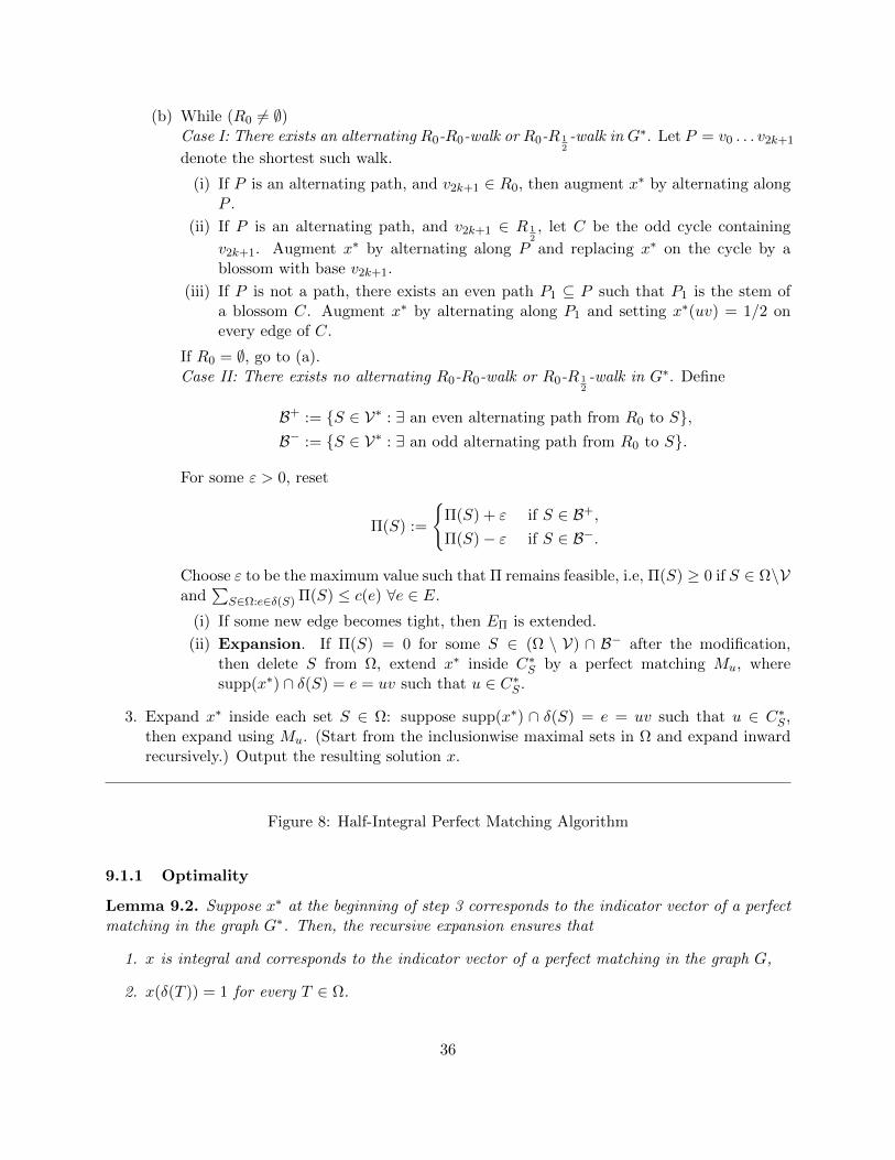
(b) While (R0 6= ∅)Case I: There exists an alternating R0-R0-walk or R0-R 1

2-walk in G∗. Let P = v0 . . . v2k+1

denote the shortest such walk.

(i) If P is an alternating path, and v2k+1 ∈ R0, then augment x∗ by alternating alongP .

(ii) If P is an alternating path, and v2k+1 ∈ R 12, let C be the odd cycle containing

v2k+1. Augment x∗ by alternating along P and replacing x∗ on the cycle by ablossom with base v2k+1.

(iii) If P is not a path, there exists an even path P1 ⊆ P such that P1 is the stem ofa blossom C. Augment x∗ by alternating along P1 and setting x∗(uv) = 1/2 onevery edge of C.

If R0 = ∅, go to (a).Case II: There exists no alternating R0-R0-walk or R0-R 1

2-walk in G∗. Define

B+ := S ∈ V∗ : ∃ an even alternating path from R0 to S,B− := S ∈ V∗ : ∃ an odd alternating path from R0 to S.

For some ε > 0, reset

Π(S) :=

Π(S) + ε if S ∈ B+,

Π(S)− ε if S ∈ B−.

Choose ε to be the maximum value such that Π remains feasible, i.e, Π(S) ≥ 0 if S ∈ Ω\Vand

∑S∈Ω:e∈δ(S) Π(S) ≤ c(e) ∀e ∈ E.

(i) If some new edge becomes tight, then EΠ is extended.

(ii) Expansion. If Π(S) = 0 for some S ∈ (Ω \ V) ∩ B− after the modification,then delete S from Ω, extend x∗ inside C∗S by a perfect matching Mu, wheresupp(x∗) ∩ δ(S) = e = uv such that u ∈ C∗S .

3. Expand x∗ inside each set S ∈ Ω: suppose supp(x∗) ∩ δ(S) = e = uv such that u ∈ C∗S ,then expand using Mu. (Start from the inclusionwise maximal sets in Ω and expand inwardrecursively.) Output the resulting solution x.

Figure 8: Half-Integral Perfect Matching Algorithm

9.1.1 Optimality

Lemma 9.2. Suppose x∗ at the beginning of step 3 corresponds to the indicator vector of a perfectmatching in the graph G∗. Then, the recursive expansion ensures that

1. x is integral and corresponds to the indicator vector of a perfect matching in the graph G,

2. x(δ(T )) = 1 for every T ∈ Ω.

36

Figure 9: The possible modifications in the Half-integral Perfect Matching algorithm.

Proof. Consider the recursive expansion in step 3. Let Ω′ denote the sets in Ω \ V that have beenexpanded until now. Let GΩ\Ω′ denote the graph obtained by contracting vertex sets in Ω \ Ω′.Recall that we expand recursively from outermost to innermost. Suppose y is an integral solutioncorresponding to the indicator vector of a perfect matching in the graph GΩ\Ω′ and y(δ(T )) = 1 forevery T ∈ Ω′. Let S be an inclusionwise maximal set in (Ω \ V) \Ω′. Since y is a perfect matching,it follows that y(δ(S)) = 1. Let e = uv ∈ supp(y) ∩ δ(S) such that u ∈ C∗S . Then, we expand yinside C∗S by using Mu. Let z be the resulting solution. Then it is straightforward to see that z isintegral and corresponds to a perfect matching in GΩ\(Ω′∪S). Thus, z(δ(U)) = 1 for each vertexU ∈ V (GΩ\(Ω′∪S)) and z(δ(T )) = 1 for every T ∈ Ω′ ∪ S. The lemma follows by induction.

Lemma 9.3. If the algorithm terminates, then the output x is a minimum-cost perfect matchingin the graph.

Proof. Upon termination, it is clear that Π is feasible to the dual program DO(G, c). We observethat x is feasible to the primal program PO(G, c). This is because, R0 ∪R 1

2= ∅ upon termination

and hence, x∗ is an indicator vector of a perfect matching in the graph G∗. Now, by Lemma 9.2, itfollows that x is also an indicator vector of a perfect matching in the graph G. To show optimality,we verify complementary slackness between x and Π.

Since the algorithm uses only tight edges to augment primal solutions, every edge in supp(x∗)is a tight edge in Π. We only need to show that the edges used in the expansion step 3 are alsotight. We observe that when a set S is added to Ω, the critical matchings that we remember forthe vertices in S use only tight edges wrt Π. Further all edges in these critical matchings inside Sstay tight until S is deleted from Ω (no change in the dual values of sets and vertices contained inS). Hence, the expansion procedure also uses only tight edges to obtain x from x∗.

Suppose Π(S) > 0 for some odd-subset S ∈ O \ V. Since the algorithm ensures that non-zerodual values are given only to subsets in Ω, we have S ∈ Ω \ V. Now, x(δ(S)) = 1 follows fromLemma 9.2.

9.1.2 Running Time

Let (x∗i ,Ωi, G∗i ) denote the triple of primal solutions, the laminar family of odd-sets Ω and the

graph G∗ at the beginning of the i’th execution of Step 2(a).

Claim 9.4. For i ≥ 1, x∗i is proper-half-integral and x∗i (δ(S)) = 1 for every vertex S ∈ V (G∗i ).

37

Proof. Our primal augmentations use only half-integral solutions that maintain the proper-half-integral property. This property is not disrupted by the expansion step during dual modification.Hence, x∗i is half-integral. It satisfies all degree constraints inG∗i , otherwiseR0(x∗i ) 6= ∅ and hence wewould not have obtained x∗i at the beginning of the i’th execution of Step 2(a), a contradiction.

At any stage of execution of the algorithm, let R0(x∗) and odd(x∗) denote the exposed verticesand the number of odd cycles respectively in the primal solution x∗.

Claim 9.5. |R0(x∗)|+odd(x∗) is non-increasing throughout the execution of Step 2(b). If |R0(x∗)|+odd(x∗) is non-decreasing, then cases I(i) and I(ii) are never executed.

Proof. This is easy to verify in both cases of Step 2(b). In Case I(i), |R0(x∗)| decreases by two. InCase I(ii), both |R0(x∗)| and odd(x∗) decrease by one. In Case I(iii), |R0(x∗)| decreases by one andodd(x∗) increases by one.

In Case II(i), we donot change x∗. In Case II(ii), it is necessary that S 6∈ R 12

(otherwise we are

in Case I(ii) and we would have augmented x∗ even before modifying the dual). Since we extendx∗ inside S using a perfect matching, we do not introduce any new cycles or exposed vertices.

For i ≥ 1, let us obtain xi by extending x∗i inside every set S ∈ Ωi \ V as follows. We extendrecursively from outermost to innermost sets in Ωi. Let Ω′ denote the sets in Ωi \V that have beenextended until now. Let GΩi\Ω′ denote the graph obtained by contracting vertex sets in Ωi \ Ω′.Suppose y is a proper-half-integral solution in the graph GΩi\Ω′ such that y(δ(S)) = 1 for eachvertex S ∈ V (GΩi\Ω′). Let S be an inclusionwise maximal set in (Ωi \ V) \ Ω′. If there exists anedge e = uv ∈ supp(y) ∩ δ(S) such that u ∈ C∗S and y(e) = 1, then we extend y inside C∗S by usingMu; if there exist two edges e1 = u1v1, e2 = u2v2, e1, e2 ∈ δ(S)∩ supp(y) such that u1, u2 ∈ C∗S andy(e1) = 1/2 = y(e2), then we extend y inside C∗S using (1/2)(Mu1 + Mu2). Let z be the solutionobtained after the extension.

Claim 9.6. The solution z is proper-half-integral in GΩi\(Ω′∪S), z(δ(u)) = 1 for each vertexu ∈ V (GΩi\(Ω′∪S)) and odd(z) = odd(y).

Proof. If there exists an edge e = uv ∈ supp(y) ∩ δ(S) such that u ∈ C∗S and y(e) = 1, then theextension ensures that the claimed properties are maintained. So, we may assume that there existtwo edges e1 = u1v1, e2 = u2v2, e1, e2 ∈ δ(S) ∩ supp(y) such that u1, u2 ∈ C∗S and y(e1) = 1/2 =y(e2). In this case, it is sufficient to verify that the number of odd cycles remains the same afterextension. For this, we observe that the symmetric difference between Mu1 and Mu2 is an evenpath between u1 and u2. Thus, all odd cycles in supp(y) which do not contain the vertex S arepreserved while the odd cycle in supp(y) containing the vertex S leads to a unique odd cycle in theextended solution.

Corollary 9.7. xi is proper-half-integral in G, xi(δ(u)) = 1 for each vertex u ∈ V and odd(xi) =odd(x∗i ).

Proof. By Claim 9.4 and inductive application of Claim 9.6.

Lemma 9.8. For every i ≥ 1, odd(xi) ≥ odd(xi+1). If odd(xi) = odd(xi+1), then cases I(i) andI(ii) are never executed in obtaining x∗i+1 from x∗i .

38

Proof. Let y∗i denote the primal solution after the ith execution of Step 2(a). Then, |R0(y∗i )| =odd(x∗i ) and odd(y∗i ) = 0 since we obtain y∗i by shrinking every cycle in supp(x∗i ) to exposedvertices. Now, the solution obtained at the end of Step 2(b) is x∗i+1. Hence, by Claim 9.5, we have|R0(x∗i+1)|+ odd(x∗i+1) ≤ |R0(y∗i )|+ odd(y∗i ) = odd(x∗i ). But R0(x∗i+1) = ∅, otherwise we would nothave obtained x∗i+1 at the beginning of i+ 1’th execution of Step 2(a). Thus, odd(x∗i ) ≥ odd(x∗i+1)and the lemma follows by Corollary 9.7. The second conclusion is also a consequence of Claim9.5.

Claim 9.9. Suppose odd(xi) = odd(xi+1). Consider an execution of Step 2(a) followed by Step2(b) to obtain x∗i+1 from x∗i . Let (y∗j , H

∗j ) denote the tuple (x∗, G∗) during the jth iteration of this

execution of Step 2(b). Let

N evenj := Set of vertices with an even length alternating walk from some vertex in R0 ∪R 1

2in H∗j ,

N oddj := Set of vertices with an odd length alternating walk from some vertex in R0 ∪R 1

2in H∗j .

We have the following conclusions:

1. If u ∈ N evenj , then u ∈ N even

j+1 .

2. If u ∈ N oddj , then either u ∈ N odd

j+1 or is expanded in some execution of case II(ii) or u is avertex in an odd-cycle in supp(y∗j ) and supp(x∗i+1).

Proof. We verify all the cases in Step 2(b). By hypothesis and by Lemma 9.8, cases I(i) and I(ii)are not executed to obtain x∗i+1 from x∗i .

In case I(iii), a new odd cycle C is created and thus, V (C) ⊆ R 12. Let P1 = v0v1 . . . v2l denote the

even alternating path with v0 ∈ R0 and v2l ∈ C. If a vertex u ∈ V (H∗j ) had an even/odd alternatingwalk from v0, then it will either have an even/odd alternating walk from v2l after modifying thesolution or u is a vertex in the cycle C. If u is a vertex in the cycle C, then u ∈ N even

j ∩ N oddj .

After primal modification u ∈ R 12

and hence u ∈ N evenj+1 . Further u is a vertex in an odd-cycle in

supp(y∗j ). Since cycles can be deleted from the primal solution only by executing the forbiddenCase I(ii), we have that u is a vertex in an odd cycle in supp(x∗i+1) as well.

In Case II, the alternating paths from vertices in R0 to vertices in B− and B+ are maintainedwhen the dual values are modified. We have to check that vertices in N even

j \ B+ and N oddj \ B−

maintain their even and odd paths from vertices in R 12

respectively. Indeed, the vertices in these

paths are disjoint from B− ∪B+, otherwise if (B−∩ N evenj ) \ B+ 6= ∅ or (B+∩ N odd

j ) \ B− 6= ∅, thenthere exists an alternating walk from a vertex in R0 to an odd cycle and hence the algorithm musthave executed the forbidden Case I(ii).

Thus, the only non-trivial case is when a set S ∈ B− is expanded. It is necessary that S 6∈ R 12,

otherwise the algorithm must have executed the forbidden Case I(ii). Thus, there exists an edgeu1v1 ∈ supp(y∗j ) ∩ δ(S), u1 ∈ S such that y∗j (u1v1) = 1. Since S ∈ B−, there exists an edgeu2v2 ∈ δ(S) that is tight wrt Π, u2v2 6= u1v1 and u2v2 lies on an odd alternating path from avertex in R0. Without loss of generality, say u2 ∈ S. Recall that we extend y∗j inside S using Mu1 .The symmetric difference between Mu2 and Mu1 consists of an even alternating path starting atvertex u2 and ending at vertex u1. Thus, vertices in N even

j and N oddj still have even and odd length

alternating paths respectively to some vertex in R0.

39

Lemma 9.10. Let Li denote the sets added to Ωi during the ith execution of Step 2(a). If odd(xi) =odd(xi+1) = . . . = odd(xj), then ∪jl=iLi ⊆ Ωj.

Proof. Consider Lk for some k = i, i + 1, . . . , j − 1. We show that Lk ⊆ Ωj . Say we executet iterations of Step 2(b) to obtain x∗k+1 from x∗k. Let S ∈ Lk. Then, S is present as a vertexin N even

1 . Then, by Claim 9.9, N even1 ⊆ N even

t . Thus, S is still present as a vertex in N event .

Consequently S is a vertex in G∗k+1 and hence Lk ⊆ Ωk+1. This already proves the statement forj = k + 1.

Next, we observe that either there exists an even alternating non-empty path from a vertex ina half-cycle in supp(x∗k+1) to vertex S in G∗k+1 or S is a vertex in a half-cycle C in supp(x∗k+1). Inthe former case, it is clear by the same argument as above that S ∈ Ωk+2. In the latter case, weobserve that V r(C) ∈ Lk+1 and hence by the above argument V r(C) ∈ Ωk+2. Now, since we deletesets from Ω in a recursive manner going from outmost to innermost (Case II(ii)), if S 6∈ Ωk+2,then V r(C) 6∈ Ωk+2, a contradiction. Thus, S ∈ Ωk+2 and consequently, Lk ⊆ Ωk+2. Iterating thisargument completes the proof.

Theorem 9.11. In the Half-Integral Perfect Matching Algorithm, Step 2(b) executes at most 2|V |−1 iterations and Step 2 executes at most (1/2)|V | log |V | iterations.

Proof. In each iteration of Step 2(b), either primal is augmented (Case I) or a set is expanded (CaseII(ii)) or the number of vertices containing even/odd alternating paths to a vertex in R0 increases(Case II(i)). The number of primal augmentations is at most |V |/2, the number of expansions isat most |Ω \ V| ≤ |V |/2 and the number of executions of Case II(i) is at most |V | − 1 since thenumber of vertices at even/odd distance from an exposed vertex increases.

Consider the execution of Step 2. By Lemma 9.8, odd(xi) is non-increasing. By Lemma9.10 and laminarity of the sets in Ωi, it follows that odd(xi) can be non-decreasing for at most|V |/2odd(x∗i ) iterations. Thus, Step 2 can execute at most (|V |/2)

∑1k=|V |/3(1/k) ≤ (1/2)|V | log |V |

iterations.

We note that naıve implementation of the Half-integral Perfect Matching algorithm could leadto sub-optimal running time. The alternating path structures across non-decreasing iterations(iterations i to j where odd(xi−1) > odd(xi) = odd(xi+1) = · · · = odd(xj) > odd(xj+1)) couldbe stored and reused. This will ensure that the number of elementary operations between twodecreasing iterations is at most O(|V ||E|). Consequently, the total number of elementary operationsperformed by the algorithm is at most O(|V |2|E|). This is the same running time complexity asthat of Edmonds’ perfect matching algorithm.

40