the computation of visible-surface representations ... · ieee transactions on pattern analysis and...

IEEE TRANSACTIONS ON PATTERN ANALYSIS AND MACHINE INTELLIGENCE, VOL 10, NO. 4, JULY 1988 417

The Computation of Visible-Surface Representations DEMETRI TERZOPOULOS, MEMBER, IEEE

Abstract-The low-level interpretation of images provides constraints on 3-D surface shape at multiple resolutions, but typically only at scattered locations over the visual field. Sparse constraints from many sources collect into visible-surface representations where, as a precursor to higher-level visual tasks, intermediate-level processing reconstructs multiscale surface shape information at every image point. This paper develops a computational theory of visible-surface representations. The visible-surface reconstruction process that computes these quantitative representations unifies formal solutions to the key problems of 1) integrating multiscale constraints on surface depth and orientation from multiple visual sources, 2) interpolating dense, piecewise smooth surfaces from these constraints, 3) detecting surface depth and orientation discontinuities to impose boundary conditions on interpolation, and 4) structuring large-scale, distributed surface representations to achieve computational eftkiency. Visible-surface reconstruction is an inverse problem. A well-posed variational formulation results from the use of a controlled-continuity surface model. Dis- continuity detection amounts to the identification of this generic model’s distributed parameters from the data. Finite element shape primitives yield a local discretization of the variational principle. The result is an emcient algorithm for visible-surface reconstruction. The algorithm deploys numerical relaxation in multigrid hierarchies and is suited to implementation on massively parallel networks of locally intercon- nected processors. Several applications contribute to an empirical evaluation of the framework.

Zndex Terns-Discontinuity detection, finite elements, multigrid relaxation, multiresolution methods, multisource integration, piecewise continuous reconstruction, regularization, variational principles, visible-surface representations.

I. INTRODUCTION VER 30 years ago, J. J. Gibson made a seminal con- 0 jecture: human visual perception in the natural en-

vironment amounts to perception of visible surfaces [26]. The representation of visible surfaces has since attracted considerable interest as an intermediate goal of computational vision. A variety of low-level visual processes participate in the recovery of the 3-D information from 2-D image data. The information contributed by each process partially constrains the shapes of visible surfaces. These constraints collect into visible-surface representations where intermediate-level processing takes place. The result is a dense, explicit description of the shapes and

Manuscript received June 7, 1985; revised December 23, 1987. Rec- ommended for acceptance by W. B. Thompson. This paper is based on MIT AI Memo 800, March 1985, by the author. Support for the Artificial Intelligence Laboratory, Massachusetts Institute of Technology, was provided in part by the Advanced Research Projects Agency of the Depattment of Defense under Office of Naval Research Contract N00014-75-C-0643 and the System Development Foundation. The author was supported by the Natural Sciences and Engineering Research Council of Canada and the Fonds F.C.A.C., Quebec, Canada.

The author is with Schlumberger Palo Alto Research, 3340 Hillview Avenue, Palo Alto, CA 94304.

TEEE Log Number 8821771.

configurations of visible surfaces. Visible-surface representations may be the basis of surface perception and they can provide quantitative information vital to higher-level surface analysis and object recognition tasks [40]. The computational vision literature describes several visible- surface representations, including depth and needle maps [34], intrinsic images [2], 2;-D sketches [41], and multiresolution representations [5 l].

This paper develops a computational approach to intermediate-level vision: The visible-sut$uce reconstruction process proposed for generating and dynamically updat- ing visible-surface representations, a generalization of the distributed, data-driven algorithm developed in [5 11, unifies the following four computational goals [52].

I) Integration: The visible-surface reconstruction process integrates local surface shape constraints from multiple sources and it fuses this information across multiple scales of resolution. The human visual system provides evidence for the importance of integration. It copes with a broad range of spatial structure in natural scenes by generating multiscale surface shape constraints through multiple spatial frequency channels [ l l]. Moreover, it coordinates two categories of low-level shape estimation processes [40] : The first, “correspondence” processes such as stereopsis and structure-from-motion, typically involves multiple image frames separated by relatively small space-time intervals. Correspondence processes triangulate interframe spatiotemporal disparities between corresponding surface features to derive depth constraints-estimates of range from the viewer to positions on visible surfaces. The second category comprises the “shape-from” processes, which can operate on single image frames. By accounting for the projective distortion of imaged surface properties such as shading, texture, and bounding contours, these processes derive orientation constraints-estimates of local surface attitude relative to the viewer. The visible-surface reconstruction process resolves ambiguities, and it counteracts the detrimental effects of noise and inaccuracies by integrating multiresolution depth and orientation constraints.

2) Interpolation: The visible-surface reconstruction process continuously propagates the integrated shape information into regions lacking shape constraints. Image representations make explicit certain local features (edges, markings, texture boundaries, etc .) correlated to salient events on physical surfaces. Since these features do not occur densely over the visual field, constraints generated by the low-level shape estimation processes will also be scattered over a subset of image points. The human visual

0162-8828/88/0700-0417$01 .OO O 1988 IEEE

418 IEEE TRANSACTIONS ON PATTERN ANALYSIS AND MACHINE INTELLIGENCE, VOL. 10. NO. 4, JULY 1988

a set of noise corrupted surface shape estimates (i.e., constraints) { c, } which can be expressed using the notation

c, = 2, [ Z ( ” ? Y ) ] + € 1 , (1) where C, denotes measurement functionals of Z ( x , y ) and E , denotes associated measurement errors, An abstract

Fig. 1 . A sparse random dot stereogram. Binocular fusion elicits a percept of dense planar surfaces. A central, opaque, textured surface is perceived suspended nearer in depth over a similarly textured background. Vivid depth discontinuities separate the dense surfaces.

system, however, systematically interprets sparse visual stimuli, such as random dot stereograms (see Fig. l) , as dense, coherent 3-D surfaces, even when the dot density is reduced so that depth is indeterminate over as much as 98 percent of the visible surface area (see, e.g., the psychophysical study [lg]). The interpolatory action of the visible-surface reconstruction process accounts for this phenomenon of ‘Ifilling in the gaps.”

3) Discontinuities: The visible-surface reconstruction process collects into discontinuity maps all low-level information about surface discontinuities, including intensity, texture, and motion boundary fragments. The process autonomously refines these maps, detecting and localizing additional surface discontinuities. Perceptually crucial are depth discontinuities, typically contours along which a surface in the scene occludes itself or another surface, as well as orientation discontinuities along creases or cusps of a continuous surface. Accordingly, random dot stereograms not only give impressions of coherent surfaces, but they also elicit vivid percepts of surface discontinuities at abrupt disparity changes (see Fig. 1). The refined discontinuity maps computed by the visible-surface reconstruction process provide (dynamic) boundary conditions which limit the interpolation of shape constraints.

4) Eficiency: The visible-surface reconstruction process must efficiently produce large quantities of numerical shape information. Visible-surface representations form and evolve in real time, in spite of the immense computational burden associated with surface reconstruction at foveal resolution. Massive, fine-grained parallelism appears to be the most viable computational architecture for this purpose. However, a characteristic limitation of massively parallel hardware is the lack of high bandwidth connections except between neighboring processors. The consequent propagation delays, however, can severely hamper global exchange of information across large visual representations. The visible-surface reconstruction process overcomes this potential inefficiency by employ- ing multiresolution relaxation within a hierarchy of surface representations each attuned to a range of spatial scales [51], [ S I .

11. MATHEMATICAL BASIS OF VISIBLE-SURFACE RECONSTRUCTION

Let the true distance from the viewer to visible surfaces be represented as z = Z ( x , y ) , a function of the image coordinates x and y . Low-level visual processes generate

statement of the visible-surface reconstruction problem is: reconstruct from the available constraints { ci } the depth function Z ( x , y ) along with an explicit representation of its discontinuities over the visual field.

A. Regularizing the Inverse Problem Visible-surface reconstruction is a nontrivial inverse

problem. First, coincident but slightly inconsistent shape estimates from different visual processes will locally overdetermine surface shape. Second, sparse constraints scattered over the visual field restrict surface shape locally, but do not determine it uniquely everywhere; there remain infinitely many feasible surfaces. Third, shape estimates are subject to errors, and high spatial frequency additive noise, regardless how small its (RMS) ampli- tude, can locally perturb the surface (orientation) radi- cally.

The inverse problem is ill-posed because the above three considerations preclude any prior guarantee that the solution will exist, or that it will be unique, or that it will be stable with respect to measurement errors. The regularization method [57], [44], [56] provides a systematic approach to reformulating this ill-posed inverse problem as a well-posed and effectively solvable variational principle.

Let X be a linear space of admissible functions. Let S ( U ) be a stabilizing functional which measures the (lack of) smoothness of a function U E X. Let 6( U ) be a penalty functional on X which provides a measure of the discrepancy between U and the given constraints. The regularized visible-surface reconstruction problem is formulated according to the following variational principle [51]:

VPl: Find U E X such that

€ ( U ) = inf € ( U ) , (2)

( 3 )

V € X

where the energy functional

I ( U ) = S ( U ) + @ ( U ) .

The solution U ( x , y ) characterizes the best reconstruction of the depth function Z ( x , y ) as the smoothest admissible function U E X which is most compatible with the available constraints. When the solution exists, it satisfies the Euler-Lagrange equations which express the necessary condition for the minimum as the vanishing of the first variational derivative 6, of the energy functional:

6 ,€ (u ) = 6,S(u) + 6 , 6 ( u ) = 0. (4) The next two sections examine S ( U ) and 6 ( U ) .

B. A Controlled-Continuity Surface Model To accomplish the reconstruction, the stabilizing func-

tional imposes generic continuity conditions on functions

TERZOPOULOS: COMPUTATION OF VISIBLE-SURFACE REPRESENTATIONS 419

admissible as possible solutions. Such conditions are ten- able inasmuch as the coherence of matter tends to give rise to continuous or smooth surfaces relative to the view- ing distance over some spatial resolution range.

Controlled-continuity stabilizers which provide local control over the continuity of the solution enable the problem to be regularized while preserving surface discontinuities. The controlled-continuity stabilizer of order 2 in two dimensions suffices in reconstructing nominally C’ continuous surfaces (continuously varying surface normal) along with explicit depth and orientation discontinuities. The stabilizer is given by

where Q C (R2 denotes the image domain, and p(x, y ) and 7 (x, y ) are real-valued weighting functions whose range is [0, 11. Assuming natural (i.e., free) boundary conditions on aQ, the variational derivative of ( 5 ) in the interior of Q is given by

where ~ ( x , y ) = ~ ( x , Y ) T ( X , Y ) and v ( x , Y ) = P ( X , Y ) [ 1 - 7 ( x , Y > l .

With S ( U ) = S,,( U ) in (3), the values of the continuity controlfunctions p ( x , y ) and ~ ( x , y ) at any point (x, y ) E Q determine the local continuity of u(x, y ) at that point: lim7(x,v) + o S,, ( U ) locally characterizes a membrane spline, a CO surface that need only be continuous; lim,(,,,,, S,,( U ) locally characterizes a thin-plate spline, a C’ surface which is continuous and has continuous first derivatives; limp(x,y) ,o S,,( U ) characterizes a locally dis- continuous surface.’ Intermediate values of p ( x , y ) and ~ ( x , y ) locally characterize a hybrid C’ “thin-plate surface under tension,” where p ( z , y ) is a spatially varying surface “cohesion” and [ 1 - ~ ( x , y ) ] is the spatially varying surface “tension” [53] , [56].

Hence, the continuity control functions p (x, y ) and ~ ( x , y ) constitute an explicit representation of depth and orientation discontinuities, respectively, over the visual field Q . A subsequent section examines the automatic identification of these functions to estimate discontinuities unknown a priori but implicit in the data { ci } .

C. A Penalty Functional

Euclidean norm A reasonable penalty functional for ( 3 ) is the weighted

@ ( U ) = ; c a i ( C i [ U ] - c i )2 , I

(7)

‘To have the intended effect on the continuity of the solution u(x, y ) to V P I , p ( x , y ) and ~ ( x , y ) must vanish on a set of nonzero measure. In the discrete formulation of the problem (see below) the finite element surface primitives automatically provide the necessary finite support.

where the a, are nonnegative real-valued constraint parameters. For CY, = l / Xu; with X a proportionality factor, this functional is in fact optimal for independently distributed measurement errors E , in (1) with zero means and variances U : .

Measurement functionals for surface reconstruction may be synthesized from point evaluation of generalized kth- order derivatikes: C, [ U ] = ( dkv/ax’ayk-’) I (X,,Y,)EZ2, for j = 0, 1, - - , k . Hence, zeroth-order (evaluation) functionals C,[v(x, y ) ] = ~(x,, y , ) serve to model the set of local depth constraints c, = ~ ( x , , y, ) + E , = d(x,,y,), for i E D . The local surface orientation, determined by the components of the surface normal n (x, , y, ) = [ U , (x, , y , ), uY (x, , y , ), - 1 1, is handled in turn by the two first- order derivative functionals C, [ U (x, y ) ] = U , (x, , y, ) and C, [ ~ ( x , y ) ] = uY(x, , y , ). This yields analogous expressions for the local orientation constraints: the set c, = U , (x, , y , ) + E , = p(,,,,, ), for i E P, and the set c, = U , (x, , y, ) + E , = q(x,,y,) , for i E Q. It is straightforward to syn- thesize additional functionals-e.g., involving directional or higher-order derivatives (for curvature constraints, etc .).

The penalty functional used in the sequel is written as

where the a, parameters are now distinguished as a&, ap,, and aq,.

D. Physical Interpretation A physical model of variational principle VPZ is illus-

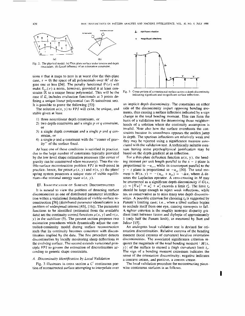
trated in Fig. 2. The controlled-continuity stabilizer models an elastic surface whose energy of deformation S,,( U ) compels its shape to vary smoothly almost everywhere (but not at discontinuities). Constraints apply forces in the z direction which deflect the surface from its nominally planar state; the penalty functional 6 ( U ) is the total deformation energy of a set of ideal springs attached to the constraints. The infrastructure of scattered depth constraints determine the deflection u(x, y ) of the elastic surface at equilibrium, as illustrated by Fig. 2(a). The height of the constraint encodes the magnitude of the local depth estimate. The tightness of each constraint is controlled by the associated spring stiffness a d i . Fig. 2(b) illustrates an orientation constraint coercing the local surface normal; the constraint parameters ap, and aq, control the spring stiffness.

E. Existence, Uniqueness, and Stability of the Solution Existence, uniqueness, and stability of the solution U (x,

y ) to VP1 are guaranteed when the functional € p T ( U ) = S,,( U ) + 6 ( U ) is a norm in the admissible space X. Now, E,,( U ) is apriori only a seminorm in X, (a particular class of Sobolev spaces); the null space 32 of func-

420 IEEE TRANSACTIONS ON PATTERN ANALYSIS AND MACHINE INTELLIGENCE, VOL. 10, NO. 4. JULY 1988

(a) (b) Fig. 2 . The physical model. (a) Thin-plate surface under tension and depth

constraints. (b) Local influence of an orientation constraint.

tions U that it maps to zero is at worst (for the thin-plate case, T = 0) the space of all polynomials over (R’ of degree one or less [56]. The penalty functional 6 ( U ) will make CpT( U ) a norm, however, provided it at least constrains X to a unique linear polynomial. This will be the case if Ci includes evaluation functionals at 3 points de- fining a unique linear polynomial (an X-unisolvent set). It is possible to prove the following [53]:

The solution u ( x , y ) to VPI will exist, be unique, and stable given at least

three noncolinear depth constraints, or two depth constraints and a single p or q constraint,

a single depth constraint and a single p and q constraint, or a single p and q constraint with the “center of gravity” of the surface fixed. least one of these conditions is satisfied in practice,

or

due to the large number of constraints typically provided by the low-level shape estimation processes (the center of gravity can be constrained when necessary). Thus the visible-surface reconstruction problem VPI is well-posed in practice: hence, for preset p (x, y ) and ~ ( x , y ) the plate/ spring system possesses a unique state of stable equilibrium-the minimal energy state u ( x , y ) .

111. IDENTIFICATION OF SURFACE DISCONTINUITIES It is natural to view the problem of detecting surface

discontinuities as one of distributed parameter identification within a variational formulation of visible-surface reconstruction [56] (distributed parameter identification is a problem of widespread interest [45], [ 161). The parameter functions to be identified (estimated from the available data) are the continuity control functions p (x, y ) and ~ ( x , y ) in the stabilizer (5 ) . The present section proposes two estimation procedures which dynamically adjust the controlled-continuity model during surface reconstruction such that its continuity becomes consistent with discontinuities implied by the data. The first procedure detects discontinuities by locally monitoring sharp deflections in the evolving surface. The second extends variational principle VPI to govern the estimation of discontinuities according to generic shape constraints.

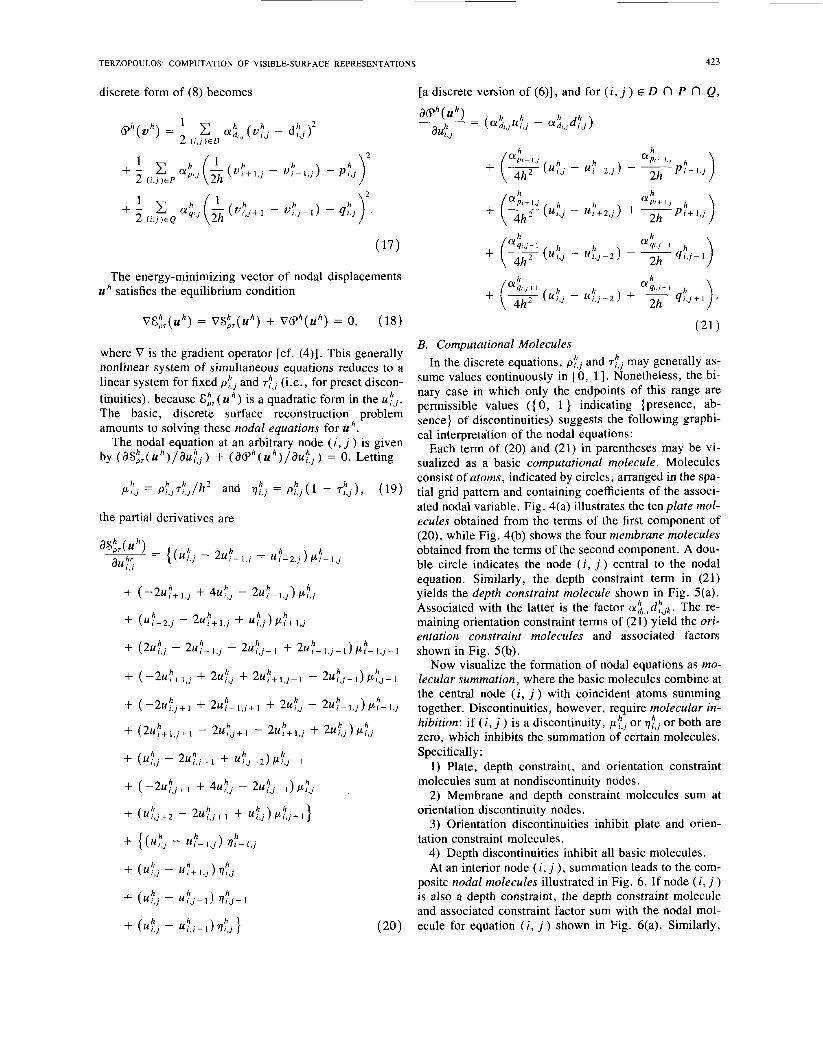
A . Discontinuity Identijication by Local Validation Fig. 3 illustrates in cross section a C’ continuous por-

tion of reconstructed surface attempting to interpolate over

L significant inflection

v insignificant inflections

Fig. 3 . Cross-section of reconstructed surface across a depth discontinuity indicating significant and insignificant surface inflections.

an implicit depth discontinuity. The constraints on either side of the discontinuity impart opposing bending mo- ments, thus causing a surface inflection indicated by a sign change in the total bending moment. This can form the basis of a validation test for determining those neighbor- hoods of a solution where the continuity assumption is invalid. Note also how the surface overshoots the constraints because its smoothness opposes the sudden jump in depth. The spurious inflections are relatively weak and they may be rejected using a significance measure associated with the validation test. A technically suitable measure having some psychophysical justification may be based on the depth gradient at an inflection.

For a thin-plate deflection function u ( x , y) , the bending moment per unit length parallel to the x - z plane is proportional to -U, , , while its counterpart parallel to the y - z plane is proportional to -uyy [50]. The total moment is M ( x , y ) = - ( U , , + uyv) = -Au , where A denotes the Laplacian operator. A zero-crossing in M may be interpreted as a significant depth discontinuity if G ( x , y ) = I V u I ’ = U ; + U ; exceeds a limit f i . The limit td should be large enough to reject weak inflections, while no1 so conservative as to miss many true depth discontinuities. A possible criterion for choosing td is suggested by Panum’s limiting case; i.e., when a tilted surface begins to occlude itself from one eye, causing stereopsis to fail. A tighter criterion is the roughly isotropic disparity gradient limit between fusion and diplopia of approximately 1 (only half the Panum limit), as measured by Burt and Julesz [15].

An analogous local validation test is devised for orientation discontinuities. Relative extrema of the bending moment (local extrema of curvature) localize orientation discontinuities. The associated significance criterion requires the magnitude of the total bending moment 1 M ( x , y ) I of the surface to exceed a (high curvature) limit to. The sign of a bending moment extremum indicates the sense of the orientation discontinuity; negative indicates a concave crease, and positive, a convex crease.

The local validation procedure for reconstructing piecewise continuous surfaces is as follows.

I

TERZOPOULOS: COMPUTATION OF VISIBLE-SURFACE REPRESENTATIONS 42 I

1) Reconstruct a tentative C' continuous surface on Q ; i.e., solve VP1 with p ( x , y ) = 7(x, y ) = 1.

2) Introduce significant depth discontinuities into the resulting surface; i.e., set p ( x , y ) = 0 at { (x, y ) 1 M ( x , y ) = 0 and G(x, y ) > td } and continue the reconstruction by solving VP1.

3) Introduce significant orientation discontinuities into the resulting surface; i.e., set ~ ( x , y ) = 0 at { (x, y ) 1 V M ( x , y ) = 0 and I M ( x , y ) 1 > t o } and continue the reconstruction by solving VP1.

4) Repeat steps 2) and 3) with decreasing td and to. Step 4) sets up an iterative continuation cycle for solv-

ing VP1, where steps 2) and 3) continue using the surface resulting from the immediately preceding step (here, (4) becomes a quasilinear equation due to the dependence of p and 7 not only on position but also on partial derivatives of U). It is wasteful to compute each approximation to high accuracy, since it serves only as an initial condition toward computing a better approximation over the suc- ceeding cycle.

The local validation procedure is reminiscent of the common practice of detecting intensity edges in image functions by applying thresholded local difference opera- tions. Since a local edge operator, such as a Laplacian, is easily corrupted by noise, a smoothing prefilter is usually applied to the image to improve the response. S,, has an analogous smoothing effect on scattered, noisy shape constraints (standard low-pass filters, such as Gaussians, are inapplicable to irregular samples). While regularization based smoothing permits the reliable computation of numerical derivatives in continuous regions [%], the smoothing property of the tentative surface computed in step 1) tends to obscure subtle discontinuities [56]. This problem is also typical of smoothing edge detection operators [39].

B. Discontinuity Identijication by Variational Continuity Con tro 1

The second discontinuity identification approach embeds VP1 within an outer variational principle which estimates the continuity control parameters p (x, y ) and ~ ( x , y ) . The surface is permitted to crease and fracture in order to reduce the total energy below the minimum ob- tainable with a globally C' surface. This resolves the con- flict between discontinuity identification and regularization smoothing.

Variational continuity control is formulated in terms of the following variational problem:

VP2: Find U, p * , and 7* such that

€(U, p* , T * ) = inf €(U, p , 7), (9) P , 7

where

€(U, P , 7) = D ( p , 7) + infE,,(v); (10)

(11)

V

q&4 = S,,(U) + @(U). Assuming suitable continuity, u ( x , y ) , p * ( x , y ) , and T* (x, y ) satisfy the coupled, nonlinear Euler-Lagrange

equations

a ay

- - ( 7 p J + 6,@(u) = 0;

- (U: + U,",] + 6,*D(p*, 7*) = 0,

(12)

with suitable boundary conditions on aQ. The functional D( p , 7) maps p ( x , y ) and 7(x, y ) into

a nonnegative energy. Its role in the outer problem is analogous to that of SpT( U) in the inner problem VP1: it serves as a stabilizer for estimating the continuity control functions from the available surface shape constraints. Locally reducing the smoothness of the surface will reduce its resistance to sudden deflections imposed by the data and hence release potential energy; i.e., from ( 5 ) , S,,( U ) considered as a function of (U, p , 7) decreases as 1 Sn p ( x , y ) dx dy and 1 So ~ ( x , y ) dx dy decrease. The introduction of discontinuities must be penalized, however, because p ( x , y ) = 0 everywhere would trivially minimize the energy. The penalty can simply increase monotonically according to a total discontinuity measure; e.g.,

7) = j j P d [ l - P(.,Y)] D

+ P o p - .(x, Y ) ] dx dY, (13 )

where pd and Po are positive energy scaling parameters for the depth and orientation discontinuity contributions, respectively.

More interestingly, D ( p , 7) can express a predisposi- tion for discontinuities arranged along piecewise continuous contours in the x - y plane (making allowances with regard to the condition in footnote 1). An appealing formulation is in terms of curvilinear controlled-continuity constraints; for instance,

the curvilinear analog of S p r , where s denotes arc length along contours c (s) = [x ( s ) , y ( s ) ] in C, a collection of discontinuity contours. Here, locally zeroing &, allows break points, while locally zeroing 0, allows tangent discontinuity points to form in the contours. Again, these events require energy penalties. Naturally, +he embedded

422 IEEE TRANSACTIONS ON PATTERN ANALYSIS AND MACHINE INTELLIGENCE, VOL. IO. NO. 4. JULY 198X

structure of the variational continuity control problem re- flects the recursive embedding of visual singularities- from surfaces to contours to points (see [56]).

Although the inner energy functional G p T ( U ) has a unique minimum for$xed p and 7 (it is quadratic, convex, and positive definite, given the conditions of Section II- E), this will certainly not be the case for G ( U , p , 7 ) in (10) which permits variation in the continuity control functions. Embedded variational problems such as VP2 are nonconvex typically and may be nondifferentiable (e.g., when the distributed parameters do not vary continuously; for instance, their range is the binary set { 0, 1 }). The rigorous treatment of such problems is the goal of nondifferentiable analysis and nonconvex optimization theory [46], [17], and is beyond the scope of the present paper. Although applicable, neither deterministic subgra- dient-type methods nor stochastic optimization techniques [2 I] have been attempted here. Instead, a discrete continuation approach is taken to solving the variational continuity control problem [61]. A subsequent section proposes an iterative procedure which efficiently computes good, although not necessarily optimal solutions.

IV. THE DISCRETE SURFACE RECONSTRUCTION PROBLEM

A closed-form solution to the variational principle for visible-surface reconstruction is infeasible due to the irregular occurrence of constraints and discontinuities. Consequently, the continuous problem is approximated by a discrete variational principle whose solution may be computed numerically. To this end, the finite element method [49], [63] is an attractive local approximation technique [5 11. As piecewise shape primitives defined in the viewer-centered coordinate system of visible-surface representations, finite elements are computationally compatible with the local depth and orientation constraints provided by the various shape estimation processes and they readily accommodate the irregular occurrence of constraints and discontinuities.

Although it is possible to discrete this problem using a variety of finite elements, including irregularly shaped isoparametric elements, the discretization will follow a regular Cartesian sampling pattern typical of images. The domain n C @i2 (assumed rectangular without loss of generality) is tessellated into square element subdomains with sides of length h . Nodes are located at subdomain corners where they are shared by adjacent subdomains. This results in a uniform Cartesian array of nodes that is well suited to VLSI implementation. The size h of the elements is adjustable so as to yield a one-to-one mapping between nodes and image pixels, as well as a geometric progression of coarser mappings. The nodes { ih, j h } n n are indexed by ( i , j ) f o r i = 1 , - * , N f a n d j = 1, . . . , NIT, where N t and N : are the number of nodes along the x and y axes, respectively.

The nodal variable v : , ~ = U ( ih, j h ) denotes the unknown displacement, or depth, at node ( i , j ). Taken together, the N h = N(: X N t nodal variables form the vector

v h E @iNh, to be determined by solving the discrete variational principle. Similarly, nodal parameters p:,j = p ( ih , j h ) and = r ( ih, j h ) represent the continuity control functions, and it is natural to interpret them as together comprising a discontinuity map in registration with the reconstructed surface.

A . The Discrete Equations The reconstructed surface is represented by an assem-

bly of square (nonconforming) finite elements E [S 11, each of which is a six-point full quadratic interpolant [see (24)]. v determines the local interpolants which explicitly represent depth and orientation everywhere over the surface. The element leads to the following 0 ( h ) finite difference type formulas for the required partial derivatives at node ( i , j 1:

Substitution of (15) along with the piecewise constant approximation p (x, y ) = pf, j and 7 ( x , y ) = T ! , ~ into (5), and noting that the area of each element is h 2 , yields the discrete functional

.

Assuming a one-to-one mapping between nodes and image pixels, the constraints coincide with nodes ( i , j ) of the grid (but not all nodes need be constrained-note, the general case of a constraint occurring arbitrarily within an element domain E may be handled easily). To obtain a discrete expression for 6 ( U ) , collect the nodes at which the various constraints occur in three sets; the set ( i , j ) E D at which depth constraints dF,j occur, and the sets ( i , j ) E P and ( i, j ) E Q at which orientation constraints p!,j and q!.j occur. Using symmetric difference approximations the


discrete form of (8) becomes

The energy-minimizing vector of nodal displacements U satisfies the equilibrium condition

V€E7(uh) = V S : T ( ~ h ) + V P h ( u h ) = 0, (18)

where V is the gradient operator [cf. (4 ) ] . This generally nonlinear system of simultaneous equations reduces to a linear system for fixed p:,; and T : , ~ (i.e., for preset discontinuities), because € E T ( U ) is a quadratic form in the U t j . The basic, discrete surface reconstruction problem amounts to solving these nodal equations for U '.

The nodal equation at an arbitrary node ( i , j ) is given by (aSET(uh) /aU3 , j ) + ( a P h ( u h ) / a u : , j ) = 0. Letting

the partial derivatives are

+ + + + + + + + + + + + +

[a discrete version of (6)], and for ( i , j ) E D fl P r l Q ,

( 2 1 ) B. Computational Molecules

In the discrete equations, plf, and rltJ may generally as- sume values continuously in [ 0, 1 ] . Nonetheless, the binary case in which only the endpoints of this range are permissible values ( { 0, 1 } indicating {presence, ab- sence} of discontinuities) suggests the following graphi- cal interpretation of the nodal equations:

Each term of (20) and (21) in parentheses may be vi- sualized as a basic computational molecule. Molecules consist of atoms, indicated by circles, arranged in the spatial grid pattern and containing coefficients of the associated nodal variable. Fig. 4(a) illustrates the ten plate molecules obtained from the terms of the first component of (20) , while Fig. 4(b) shows the four membrane molecules obtained from the terms of the second component. A double circle indicates the node ( i , j ) central to the nodal equation. Similarly, the depth constraint term in (21) yields the depth constraint molecule shown in Fig. 5(a). Associated with the latter is the factor ~ ! 2 ~ , d f t , ~ . The re- maining orientation constraint terms of (21) yield the orientation constraint molecules and associated factors shown in Fig. 5(b).

Now visualize the formation of nodal equations as molecular summation, where the basic molecules combine at the central node ( i , j ) with coincident atoms summing together. Discontinuities, however, require molecular inhibition: if ( i , j ) is a discontinuity, pLltJ or q:,J or both are zero, which inhibits the summation of certain molecules. Specifically:

1 ) Plate, depth constraint, and orientation constraint molecules sum at nondiscontinuity nodes.

2) Membrane and depth constraint molecules sum at orientation discontinuity nodes.

3) Orientation discontinuities inhibit plate and orientation constraint molecules.

4 ) Depth discontinuities inhibit all basic molecules. At an interior node ( i , j ), summation leads to the com-

posite nodal molecules illustrated in Fig. 6. If node ( i , j ) is also a depth constraint, the depth constraint molecule and associated constraint factor sum with the nodal molecule for equation ( i , j ) shown in Fig. 6(a). Similarly,

424 IEEE TRANSACTIONS ON PATTERN ANALYSIS AND MACHINE INTELLIGENCE, VOL. IO. NO. 4, JULY 1988

(b)

Fig. 4. (a) Plate molecules. (b) Membrane molecules.

- Q P k J + l Ih q * s J + l

QL A -- Ih q t a J - 1

(b) Fig. 5. (a) Depth constraint molecule. (b) Orientation constraint mole-

cules.

the upper left molecule in Fig. 5(b) sums with the nodal molecule only if ( i - 1, j ) E P, the upper right only if ( i + 1 , j ) E P, the lower left only if ( i , j - 1 ) E Q , and the lower right only if ( i , j + 1 ) E Q. Fig. 7 illustrates nodal molecules which can result from inhibition by discontinuities.

Discretizing u ( x , y ) , p(x, y ) , and 7 ( x , y ) over the same grid of nodes is convenient for expressing the nodal equation. However, it is more natural to position depth discontinuities on the links half way between nodes p;,, = p ( k h + ( h / 2 ) , lh + ( h / 2 ) ) , since u : , ~ is undefined at a depth discontinuity. Orientation discontinuities can remain coincident with nodes 7 t j = 7 ( ih, j h ) (since u t j is defined at an orientation discontinuity). Generally, a discontinuity inhibits a molecule if it coincides with a con- stituent atom or link.

Variants of the above summation and inhibition rules

(a) (b) Fig. 6 . Interior nodal molecules. (a) Molecule at node ( i , j ) away from

constraints and discontinuities (here p;,, = T:,, = 1 and nodal equation is (20/h2)u:,, - (8/hZ)(u:-l , , + u~+I,, + u?,-I + & + I ) + (2 /h2 ) (u : -~ , , - l + u~+I.,-I + ~!-I,,+I + ~ ! ' + I , , + I ) + ( l / h 2 ) (U:-*,, + u:+~,, + u : , - ~ + = 0). (b) Molecule at interior orientation discontinuity node ( i , j ) (here .:] = 0 and nodal equation is4u!', - ut-,,, - ut+,,, - u t l - , - u ! ' ~ + ~ = 0). Note that molecules represent h 2 times 13-point finite difference approximation to biharmonic (thin plate) operator and 5-point approximation to Laplacian (membrane) operator [ l , p. 8851.

X

X

X

X

X

X

(b) Fig. 7. Molecular inhibition at discontinuities. (a) Nodal molecules at

boundary nodes (double circles) near depth discontinuity nodes (X's). (b) Nodal molecules at boundary orientation discontinuities (double circles) next to depth discontinuities (X's).

are possible. One useful alternative is to create horizontal or vertical depth discontinuities by introducing adjacent orientation discontinuities that inhibit only the "( -2 ) - (4)-( -2)" molecules in Fig. 4.

C. Nodal Computations and Multiresolution Relaxation The system of nodal equations features computationally

desirable properties: its matrix becomes positive definite

TERZOPOULOS: COMPUTATION OF VISIBLE-SURFACE REPRESENTATIONS

coarse

1 medium

1 fir

+ fine

+ coarse medium

Fig. 8. Structure of the multiresolution surface reconstruction algorithm. Iterative relaxation processes propagate information within each level. Coarse-to-fine (prolongation) and fine-to-coarse (restriction) processes transfer information between levels. Synthetic orientation and depth constraints consistent with a hemispherical surface are input (top). Algo- rithm computes dense multiscale surface representation (bottom).

[for fixed p ( x , y ) and 7(x, y ) ] as soon as the available constraints satisfy the conditions for a well-posed problem. Moreover, the matrix is sparse (entries predomi- nantly zero), banded, and symmetric, due to the local support of the finite element representation. However, its size N h X N h may become extremely large, since the number of pixels N h in typical images can range from lo4 to lo6 or greater. This combination of properties suggests the application of iterative techniques which exploit sparsity, such as relaxation methods [32].

A parallel (Jacobi-type) nodal relaxation computation at node ( i , j ) may be written as follows:

where the bracketed superscripts contain the iteration index and w is a (time) step size. The aforementioned molecular summation and inhibition rules fully automate the node-by-node construction of the bracketed term in this local-support computation. The computation is spatially

__

425

noninvariant and it changes temporally according to perturbations in the local structure of constraints and discontinuities. Gauss-Seidel nodal relaxation computations can be constructed similarly, as was done in [51].

For large problems the nodal relaxation computations usually suffer from very slow convergence. There exist efficient algorithms based on multigrid relaxation methods [3 I] for a number of visual problems [ S I , including interpolation problems involving globally continuous thin- plate splines [5 I]. The multiresolution relaxation approach is well suited to the visible-surface reconstruction process. Fig. 8 illustrates the structure of a three-level instance of the multiresolution surface reconstruction algorithm. A considerable simplification of the computations results from a 2: 1 resolution reduction between adjacent levels (members of the hierarchy of embedded finite element subspaces). The hierarchy of representations and component processes are coordinated to increase computational efficiency. A recursive coordination strategy (see, [51], [ S I ) was employed in the experiments described below.

V. EXPERIMENTS WITH THE ALGORITHM The multiresolution visible-surface reconstruction al-

gorithm was tested on a variety of data sets including synthetic data, structured light (laser) rangefinder data, au- tomated stereopsis and photometric stereo data from natural images, and digital terrain model data. This section presents selected results ([53] contains more examples and further details). For all the examples presented, the intralevel process was Gauss-Seidel relaxation and the algorithm was started from zero initial approximations on all the levels. Discontinuity maps have preset borders of depth discontinuities to introduce natural (free) boundary conditions.

A. Experiments Involving Preset Discontinuities Synthetic Data: The first two examples illustrate mul-

tiresolution, piecewise continuous surface reconstructions from randomly placed depth constraints and prescribed discontinuities. Fig. 9 presents the reconstruction of a circular shell and Fig. 10 presents the reconstruction of stacked circular planes. Fig. 11 shows the reconstruction from orientation constraints of a pyramidal surface with orientation discontinuities. Fig. 12 presents the reconstruction of a hemispherical surface from scattered orientation constraints. Since it is impossible to determine absolute depth solely from Orientation constraints, a relative-depth reconstruction results, with the center of gravity of the reconstructed surface resting near the x - y plane. However, the integration of depth constraints with orientation constraints determines the absolute depth of the surface, as illustrated by Fig. 13. The constraint values in this latter example are corrupted by uniformly distributed noise. With the constraint parameters chosen, the surface is slightly bumpy on the finest level; the bumpi- ness can be reduced by decreasing the constraint parameter values (loosening the springs of the physical model).

426 IEEE TRANSACTIONS ON PATTERN ANALYSIS AND MACHINE INTELLIGENCE, VOL. IO. NO. 4. JULY 1988

Fig. 9. Multiresolution reconstruction of a shell from depth constraints. (a) Constraints obtained by randomly sampling at three resolutions a hemisphere with z values scaled by a radial sinusoid. Nodes outside circular region occupied by constraints were preset depth discontinuities. (b) Reconstructed surface representation. (Grid dimensions: N:' = N!' = 17, N F = N: = 33, N!!' = N: = 65. Grid spacings: h , = 0.4, hz = 0.2, h3 = 0.1. Constraint density: 15 percent. Constraint parameters: a ) = 2.0 /hJ . Computation: 24.25 work units. A work unit i s the amount of computation required per relaxation iteration on the finest level.)

Fig. 11. Multiresolution reconstruction of a pyramidal surface from orientation constraints. (a) Constraints at three resolutions-values are constant within each quadrant. Nodes along quadrant boundaries are preset orientation discontinuities. Outer nodes are present depth discontinuities. (b) Reconstructed surface representation. (Grid dimensions: N,h' = N:' = 17, NF = NF = 33, N? = NY = 65. Grid spacings: h , = 0.4, h, N = 0.2, h, = 0.1. Constraint density: 100 percent. Constraint parameters: ct; = ct? = 4.0/h,. Computation: 19.5 work units.)

Fig. 10. Multiresolution reconstruction of stacked circular planes from depth constraints. (a) Constraints obtained by randomly sampling the planar surfaces at three resolutions. Depth discontinuities are placed along circular arcs bounding the planes and along the outer edges of the grids. (b) Reconstructed surface representation. (Grid dimensions: N t ' x = 22 x 17, N? x N:2 = 43 X 33, N? x N:" = 85 X 65. Grid spacings: h , = 0.4, h - 0.2, h3 = 0.1. Constraint density: 15 percent. Constraint parameters? 3 = 2.0 /hJ . Computation: 20.375 work units.)

Fig. 12. Multiresolution of a hemisphere from orientation constraints. (a) Constraints randomly sampled at three resolutions from a hemisphere. Nodes outside the hemispherical surface patch were preset depth discontinuities. (b) Reconstructed surface representation. (Grid dimensions: N:' = N:' = 17 Nh' = Nh2 = 33, N? = N:' = 65. Grid spacings: h , = 0.4, h2 = 0.2, h, = 0.1. Constraint density: 30 percent. Constraint parameters: a; = a$ = 4.0/h,. Computation: 22.125 work units.)

, x v


\/

\ ' / \ / \

Fig. 14. Reconstruction of a light bulb from range data. (Finest grid dimensions: N P X N T = 257 x 281. Grid spacings: h , = 0.8, hz = 0 . 4 , h3 = 0 . 2 , and h4 = 0.1. Constraint parameters: a$ = 0 . 2 / h , . Compu- tation: 9.78 work units.)

v v (a) (b) (C)

Fig. 13. Multiresolution reconstruction of the hemisphere from depth and orientation constraints. (a) Depth constraints and (b) orientation constraints consistent with a hemisphere at three resolutions. (c) Recon- structed surface representation; note the absolute height above the base plane is obtained. (Grid dimensions: Ng' = NC' = 17 Nh* = Nh* = 33, NI' = N: = 65. Grid spacings: h, = 0.4, h, = 0.2, h, = 0.1. Constraint density: 15 percent. Constraint noise: 10 percent uniform. Constraint parameters aifl = 2 . 0 / h , , a? = a% = 4 . 0 / h , . Computation: 17.75 work units.)

' 1 Y

Structured Light Data: The multiresolution algorithn, was applied to the reconstruction of several objects from raw range data supplied by a laser rangefinder constructed at MIT by P. Brou. The scan resolution in the y direction is half that in the x direction. The examples involve a four-level surface reconstruction algorithm. The raw rangefinder data were introduced as depth constraints at the

cessive 2 X 2 averaging between levels. To expediently finest level and transferred to the coarser levels by sue- . . . . . s , , . . . ~ . . , . .

\ /

segment the objects from the supporting platform, values smaller than a threshold were treated as depth discontinuities. Fig. 14 shows the reconstructed surface of a lightbulb. The algorithm smoothes the noise in the data and reconstructs the missing points.

Photometric Stereo Dura: The surface reconstruction algorithm provides a noise resistant technique for computing depth from the surface orientation data provided by photometric stereo [62]. This is demonstrated using the image of a toroid (Fig. 15). The photometric stereo data shown (generated by a program implemented at MIT by K. Ikeuchi) were introduced as orientation constraints on a two-level algorithm. Aside from sporadic missing data, the constraints on the coarse level are dense, while only every other node on the fine level is a constraint. Fig. 15(c) shows the reconstructed toroid.

Correlation-Based Stereo Data: Fig. 16(a) shows a stereopair that was input to the correlation-based stereo program described in [36]. Fig. 16(b) shows the output of the program. The neutral gray patches indicate regions of unknown disparity, where the algorithm has failed to produce a match. Successively averaging by factors of two, subsampled versions of the disparity data on the finest

\ / (b) (C)

Fig. 15. Reconstruction of a torus from photometric stereo data. (a) Image of a matte white toroid. (b) Orientation constraints provided by photometric stereo. (c) Reconstructed torus. (Grid dimensions N:' = N:' = 51 and N: = Nh,2 = 101. Constraint parameters: cyhJ = 4 . 0 / h , . Com- putation: 52.0 work units.)

level were introduced as input to the multiresolution algorithm on three coarser levels. Relatively small constraint parameter values were chosen in order to counter- act the false matches and noise present in the disparity data. Fig. 16(c) shows the reconstructions on the three coarsest levels as 3-D plots (the finest level was too dense to render as a wire frame surface). Fig. 16(d) shows isoelevation contour maps of the solution on all levels.

Fig 16. Kccon\truction of terrain f rom corrclation-based stereo data. ( a ) Natural terrain stcropair iinia@e\: 256 X 256 pixels. quantized to 2.56 gra) l e ~ c l s : courte\) ot U . S . Defense Mapping Agency). ib) Output of corrclation-b;i\ed \ t e rm program ibrightnes\ proportional to di\parit> : disparit? unknou n in ncutral prek regions). ( c ) Reconstructed terrain on three coarsest I zvc ls . i d ) lsoclevation contour maps. (Grid dimensions:

= 3 3 , ,yt: ,p? = 65 . = ,p = 129, = = 157, ings; / I , = 0.8. h , = 0.4. / I , = 0.2. / I , = 0.1. Constraint

parameter5 aC, = 0.01 //I,?. Computation 29.0 work units.)

FcarurcJ-Busecl Stereo Datu: The stereopair of Fig. 17(a) was input to a three-channel version of the (zero- crossing) feature-based stereo program described in [ 291. Fig. 17(b) shows the output of the program. Disparity information is available only along zero crossing contours at the three finest scales. This disparity data were input to a four-level surface reconstruction algorithm, with the constraints on the coarsest level derived by averaging the constraints from the next finer level. Fig. 17(c) shows the reconstructions on the three coarsest levels as 3-D plots. Fig. 17(d) shows isoelevation contour maps of the solution on a l l levels.

Digital Terruiti M u p Dtrtu: Fig. 18 presents the application of a four-level surface reconstruction algorithm to contoured terrain elevation data. The data was generated by J . Mahoney, using a digitizing tablet to trace manually

the isoelevation contours in a map of the Black River Gorges (published by the UK Ministry of Defense). Fig. 18(b) shows contour plots of the reconstructed terrain on all levels. The elevations of the reconstructed contours are chosen halfway between the original constraint contours of Fig. 18(a) to avoid favorable bias. The reconstructed contours are somewhat smoother than the contours in the published map. The jaggedness introduced by manual digitization has been reduced: the constraint parameters regulate the smoothing. Fig. l8(c) shows shaded images of the reconstructed terrain. Comparison of terrain reconstructions using the controlled-continuity model against reconstructions using a simpler membrane spline model (Laplacian smoothing) indicates that the latter generally suRers from insufficient smoothness and produces Rat spots across terrain peaks (see also 191).

TERZOPOULOS. COMPUTATION OF VISIBLE-SURFACE REPRESENTATIONC 429

I I

Fig. 17. Reconstruction of terrain from feature-based stereo data. (a) Nat- ural terrain stereopair (images: 512 x 512 pixels, quantized to 256 levels; courtesy of US Army Engineer Topographic Labs). (b) Output of feature-based stereo program (contour intensity proportional to disparity). (c) Reconstructed terrain on three coarsest levels. (d) Isoelevation contour maps. (Grid dimensions: N2’ = N:’ = 33, N:’ = N t 2 = 65, N!’‘ = N(” = 129, N F = NI” = 257. Grid spacings: h , = 0.8, h, = 0.4, h, = 0.2, h., = 0.1. Constraint parameters: a) = O.OI/h:. Computa-

B. Discontinuity Idenr$cation

tion: 3 I .O work units.)

Experiments

When all discontinuities are preset, the discontinuity map, p:.j = p ( i h , j h ) and T:, = ~ ( i h , j h ) , comprises a fixed part of the input data. More generally, some or all of the discontinuities are unknown, so the discontinuity map undergoes refinement during surface reconstruction. The following experiments involve the automatic identification of surface discontinuities, first by local validation, followed by variational continuity control (refer to Section 111).

Local Validation: Fig. 19 illustrates the application of the local validation method to a random dot stereogram. Fig. 19(b) shows the depth constraints generated by a three-channel version of the feature-based stereo program [29]. The discontinuities identified using one cycle of lo-

cal validation are superimposed onto the final disparity maps in Fig. 19(c). Fig. 19(d)-(g) illustrates the steps of the local validation method in more detail. Fig. 20 illustrates a similar experiment using an aerial view stereopair. The results demonstrate the feasibility of identifying significant discontinuities using local validation, but the interpolation process can be seen ‘‘leaking” through gaps due to undetected discontinuities. No single value of the global limit td can be expected to produce perfect results, especially with natural imagery. As was suggested in Sec- tion 111-A, however, decreasing the disparity gradient limit in a sequence of cycles, iterating to near-equlibrium each time, will elicit increasingly shallow discontinuities.

Variational Continuity Control: Variational continuity control involves a similar multistep strategy guided by the energy functional E ( U , p , 7) in VP2. The present imple-

1.1 '

I. I

Fig. I X Kecon\truction of digitctl terrain map datu ( a ) 256 X 756 dipital contour arra) input to algorithm Icontour hrightne\s proportional to el- e\iition: Ioc;iI a\eraging 0 1 tinest grid > ieldeil con\tr:iint\ on c o a r w r grid\: patch to Ioucr right indicates ;I lake). (h) Reconstnicted i\oelev;ition contour map. ( c ) Shaded terrain representation\. (Grid Dimensions: A'!

\pacing\: / I , = 0 . X . 11, = 0.4. / I ; = 0 .7 . / I , = 0.1. Constrnint paromc- t u \ : (y:: = 0.5 l iL.1

= ,vr' ~ = . . . 7 3 VI' ~ = ,\?! = 6 5 , , V t = ,Vt = 179. ,VJt- z \:. = 3 7 , Grid

mentation employs the following discrete form for the discontinuity functional a ( p , 7 ) in ( I O ) :

whcre D(i, and Oii, are relative potential cner, cries of local discontinuity configurations in the depth and orientation discontinuity maps. respectively. Fig. 2 1 illustrates some con fi g u rat ions and as soc i a ted e ne rg i e s chose n he u ri s t i - cally to favor the formation of continuous and smoothly curving discontinuity contours; higher energies are as- signed to i so I a ted disco n t i n u i t i e s . term i nation s. s harp bends. junctions, and discontinuity clumps ( 2 5 1 .

The strategy for "solving" VP2 is 21s follows: The outer iteration consists of 1 j each continuity control parameter pi!, or ~ j j , (in parallel) flips its value in { 0. 1 } if this rc- duces the energy E" ( I O ) . then 3 ) given the updated p i ' , or

7/1,. the basic surface reconstruction algorithm obtains the unique minimum of the inner functional ( 1 1 ) . First. the outer itcrution identifies depth discontinuities. with 6;; ini- tially set to a high value (to heavily penalize fracture). then gradually lowered. Next, the outer iteration identifies orientation discontinuities with 0:: decreasing in the same way. Orientation discontinuity identification is de- layed. otherwise the small surface inflections occurring near undetected depth discontinuities (see Fig. 3 ) are easily misconstrued as orientation discontinuities, which re- tards the optimization process. Fig. 22 illustrates the variational continuity control approach using a synthetic

The above describes a continuation procedure (6 I ] for solving VP2. in which 3:; and 13:: serve as continuation variables. VP2 becomes increasingly convex-i.e.. simpler-for larger values of these variables. By gradually

example.

TERZOPOULOS: COMPUTATION OF VISIBLE-SURFACE REPRESENTATION< 429

I

Fig. 17. Reconstruction of terrain from feature-based stereo data. (a) Nat- ural terrain stereopair (images: 512 x 512 pixels, quantized to 256 levels; courtesy of US Army Engineer Topographic Labs). (b) Output of feature-based stereo program (contour intensity proportional to disparity). (c) Reconstructed terrain on three coarsest levels. (d) Isoelevation contour maps. (Grid dimensions: NI(' = N:" = 33 , NI(' = Nt' = 65, N t ' = N:' = 129, N? = N:" = 257. Grid spacings: h , = 0.8, hz = 0.4, h , = 0.2, h , = 0.1. Constraint parameters: a:; = O.OI/h:. Computa- tion: 31.0 work units.)

B. Discontinuity IdentiJcation Experiments

When all discontinuities are preset, the discontinuity map, pjf, = p ( i h , j h ) and r:, = 7 ( ih, j h ) , comprises a fixed part of the input data. More generally, some or all of the discontinuities are unknown, so the discontinuity map undergoes refinement during surface reconstruction. The following experiments involve the automatic identification of surface discontinuities, first by local validation, followed by variational continuity control (refer to Section 111).

Local Validation: Fig. 19 illustrates the application of the local validation method to a random dot stereogram. Fig. 19(b) shows the depth constraints generated by a three-channel version of the feature-based stereo program [29]. The discontinuities identified using one cycle of lo-

cal validation are superimposed onto the

(C)

final disparity maps in Fig. 19(c). Fig. 19(d)-(g) illustrates the steps of the local validation method in more detail. Fig. 20 illustrates a similar experiment using an aerial view stereopair. The results demonstrate the feasibility of identifying significant discontinuities using local validation, but the interpolation process can be seen "leaking" through gaps due to undetected discontinuities. No single value of the global limit td can be expected to produce perfect results, especially with natural imagery. As was suggested in Sec- tion 111-A, however, decreasing the disparity gradient limit in a sequence of cycles, iterating to near-equlibrium each time, will elicit increasingly shallow discontinuities.

Variational Continuity Control: Variational continuity control involves a similar multistep strategy guided by the energy functional G ( U , p , 7) in VP2. The present imple-


Fig. 20. Local validation applied to piecewise continuous stereo reconstruction. (a) Aerial view stereopair of a hospital complex (images courtesy of U . British Columbia, Faculty of Forestry). (b) Disparity contours on finest level (size 320 x 320) generated by feature based stereo program (darkness proportional to disparity). (c) Full disparity map generated by surface reconstruction algorithm on finest level. (d) Disconti- nuities identified on finest level (white contours) superimposed on reconstructed piecewise continuous disparity map.

additional energy [this occurs in the transition from Fig. 22(f) to (g)]. Although it has achieved the global optimum of VP2 in Fig. 22(h), the continuation procedure can generally be expected to yield good, although not necessarily optimal solutions. Its deterministic nature and efficiency are attractive.

VI. DISCUSSION This paper has developed a computational theory of vis-

ible-surface representations. The visible-surface reconstruction process which implements the theory provides a uniform treatment of integration, interpolation, discontinuities, and efficiency, the four computational goals out- lined in the introduction. The concluding discussion sur- veys research directly relevant to the computation of

Fig. 21. Some local discontinuity configurations and associated relative energies. Circles represent npdes ( i , j ), while X's denote discontinuities (positions where ph or T~ are 0; depth discontinuities occur on links between nodes while orientation discontinuities coincide with nodes.) (a) Energies Dfi, for depth discontinuity configurations (cf. [25] ) . (b) Ener- gies Ofi, for some orientation discontinuity configurations. Rotating configurations by increments of 90 degrees leaves associated energies unaf- facted.

(g) (h) Fig. 22. Variational continuity control method for piecewise continuous

reconstruction. (a) Scattered depth constraints consistent with sloping planes meeting discontinuously. (b) Globally C' reconstructed surface obtained with high /32 and /3:. Note smeared depth discontinuities and rounded orientation discontinuities. (c)-(h) Evolution of the variational continuity control process. /32 is lowered first to identify depth discontinuities (c)-(g) is lowered next to identify orientation discontinuities. (h) Final piecewise continuous surface.

TERZOPOULOS: COMPUTATION OF VISIBLE-SURFACE REPRESENTATIONS 43 I

Fig. 19. Reconstruction of a random dot stereogram by local validation. (a) Synthesized stereogram of four planar surfaces stacked in depth. (b) Depth constraints for random dot stereogram (finest level dimensions: 320 x 320; constraints on coarsest level obtained by averaging from finer level). (c) Piecewise continuous disparity maps with detected discontinuities (white contours) superimposed. (d)-(g) Local validation method on a coarse level. (d) Reconstructed C’ surface. (e) Zero crossings of discrete bending moment MI’, = - l / h 2 ( u f ’., + U?+‘,, +

I + U:,,+, - 4uii, 1 (black points). ( f ) Significanct zera crossings for which Glj, > rei with I , ~ = I , where G:!, = 1 / 4 h 2 [Cui’+ ,,, - U:- )’ + iuii,+ I - U::,- I )!I. (g) Piecewise continuous surface results from inserting latter into discontinuity map (by setting associated p:! , to zero) and continuing iterative reconstruction process.

decreasing /32 and /3::, a trajectory is followed from the computation may be concentrated at nodes near modified optimum of the simple problem towards a satisfactory discontinuities). Increasingly accurate discontinuities “solution” to the difficult, nonconvex target problem emerge as 0: and 0; decrease. Once a true discontinuity ( /3: and small). In general, relatively few of the pll j or appears it tends to persist (a hysteresis effect); thus, be- ~ f l , are observed to change at each step, so few iterations yond some minimal 6; and 0; values, a slight increase are necessary per step (in a uniprocessor implementation, will eliminate some spurious discontinuities and release

434 IEEE TRANSACTIONS ON PATTERN ANALYSIS AND MACHINE INTELLIGENCE, VOL. IO, NO. 4, JULY 1988

piecewise continuous reconstruction, although the formulation presents difficulties, especially with regard to estimating irregular discontinuities in multidimensions [48]. In view of the requirements specific to the computation of visible-surface representations-very large constraint sets, undetermined discontinuities, desirability of massively parallel implementation, etc. -it appears pref- erable to apply finite element techniques which yield sparse systems of equations, as is done in the present paper.

Barrow and Tenenbaum [3], [4] use relaxation while Grimson [27], [28] uses standard optimization algorithms for surface interpolation. These iterative algorithms have parallel variants which are thought to be “biologically feasible. ” However, their tendency to be poorly condi- tioned, even for reconstruction problems of moderate size, results in very slow convergence. Excruciatingly slow convergence also limits the size of problem that can be attempted with optimization via simulated annealing [25], [42]. Terzopoulos [5 11 shows that multiresolution surface reconstruction based on multigrid relaxation methods ac- celerates convergence dramatically while maintaining bi- ological feasibility. Cochran and Medioni [ 191 describe another implementation of this multiresolution surface reconstruction algorithm. An efficient multigrid algorithm for reconstructing surfaces from shaded monocular images is described in [ S I . A concurrent multigrid coordination strategy which solves a coupled, multilevel version of the variational principle is developed in 1541; the approach is well suited to massively parallel hardware because it maintains simultaneous processor activity in all levels.

B. Research Directions Alternative organizations of shape information in visi-

ble-surface representations are worthy of further study. One possible variant is a relative shape representation, where only the coarsest grid contains absolute depth and orientation values, while each finer grid contains increasingly detailed perturbations relative to the sum of these values over all coarser grids. Surface structure parsimon- iously decomposes into the hierarchy of finite element subspaces of the multiresolution representation (roughly analogous to a Fourier decomposition). A relative shape representation may simplify the multigrid relaxation algorithm by enabling the levels to run virtually independently of one another (see [53, Ch. 111 for a detailed discussion). Another representation of interest is the explicit depth/slope representation proposed in [33].

The coupling of visual constraints to the surface model requires further analysis. The surface model can be re- lated to expectations regarding the class of admissible surfaces, and a connection exists between the constraint parameters ai and the statistical properties of noise or in- accuracy in the data [56]. Assuming that low-level visual processes can associate a confidence or variance estimate with each shape constraint, it appears possible to systematically assign appropriate values to the constraint param-

eters. In particular, cross validation techniques [60] may provide a means of setting X -’ [refer to text after (7)] to optimally tune the smoothness of the reconstructed surface according to the noise present in the data.

The arbitration of visible-surface reconstruction by higher-level processes has received insufficient attention. Among other important functions, an arbitrator could deal with occasional outliers or massively inconsistent data by nullifying individual or entire sets of constraint parameters. The straightforward treatment of a particular kind of rivalry, that due to transparent surfaces is described in [53, Ch. 1 1 1 . The arbitrator monitors the approximation error betwen reconstructed surface and shape constraints over broad areas. An excessive error triggers a grouping process which clusters constraints. Multiple surfaces are then reconstructed over the same region, one for each ho- mogeneous constraint population.

The line processes used in the discontinuity detection experiments are rather primitive. Zucker and Parent [65] employ a more sophisticated discrete encoding of local orientation in a relaxation labeling algorithm for contour detection in images. It appears possible to employ a similar encoding in the estimation of surface discontinuities by variational continuity control via VP2. A continuous encoding of the local orientations of curvilinear boundary elements appears even more desirable, but introduces additional real-valued nodal parameters in the discontinuity map.

Analog computation by electrical networks [35] is an attractive approach to generating visible-surface representations. The major advantages of large analog networks are fault tolerance, noise dissipation, and very rapid set- tling to steady-state (within a few network time con- stants). Lumped analog networks may be designed systematically whose steady-state voltages and currents represent quantities of interest in variational formulations of visual problems such as surface reconstruction [53], [44], [37], [33]. The network design process parallels finite element discretization; one or more electrical devices may be used to simulate the physical properties of each finite element [63]. Resistance networks for computing first order and second order spline interpolants are shown in Fig. 23.

It remains to explore ensuing processes that generate stable higher-level shape descriptions which are better tuned to object recognition. The visible-surface representation comprises only an intermediate, viewer-centered description of the 3-D surfaces in scenes, and the goal of subsequent processing is to abstract a rich set of object- centered features that are stable through viewpoint changes. This goal begins with visible-su~ace analysis, which is facilitated by the dense, quantitative shape information provided by visible-surface representations. This topic is considered further.

A promising approach to visible-surface analysis is to apply concepts from differential geometry [20]. For instance, according to the fundamental theorem of the local theory of surfaces (Bonnet), the analytic study of a sur-


Fig. 23. Analog networks for harmonic and biharmonic interpolation. (a) Network of resistances r = 1 / h 2 solves Poisson’s equation for displacement (depth) over a uniform grid of spacing h . Currents g,,, determined by the right-hand side of the equation are injected into each node. Volt- ages are applied to certain nodes in accordance with the boundary conditions and constraints of the problem. Discontinuities may be inserted by “breaking” resistors. (b) Two cascaded networks solve the biharmonic equation over a uniform grid. Top network solves a Poisson equation for the bending moment, while bottom network solves a similar equation for the displacement.

face consists of the study of its two fundamental forms; i.e., the six fundamental tensor coefficients (not all independent) as functions of the two independent parame-

Fig. 24. Computing intrinsic and extrinsic surface properties in the visible-surface representation. (a) Computed Gaussian curvature K,,, of reconstructed lightbulb at four scales. Elliptic points (K > o ) are white, hyperbolic points ( K < 0) are black, and parabolic points ( K = 0) separate regions. (b) Computed principal direction field for reconstructed lightbulb at the two coarsest scales showing directions of greatest curvature (left) and least curvature (right).

ters of the surface. The fundamental forms are invariant under changes in surface parameterization, and together they determine surface shape up to rigid body transfor- mations, making them ideal foundations for object-centered representations of surfaces [53, Ch. 111.

The finite element shape representation reduces the computation of fundamental forms and derived surface features such as the Gaussian, mean, and principal curvatures to the evaluation of simple algebraic expressions of neighboring nodal variables [see Appendix, (25)-(28)]. It therefore becomes straightforward to compute the elliptic, hyperbolic, parabolic, umbilic, and planar points, as well as geodesics, asymptotes, and lines of curvature. Fig. 24 illustrates some of these computations using the reconstructed surface of the lightbulb. The results demonstrate the feasibility of reliably computing from visible-surface representations higher-order intrinsic and extrinsic properties of surface shape (see also, e.g., [12], [22], [51, [59]) . The reliability is attributable to the controlled-continuity surface model which overcomes the potentially


detrimental effects of noise in the data without destroying discontinuities.

where

I XI x x2l APPENDIX

Denote a vector in cR3 by x = [x', x 2 , x3], and a surface patch by x = x ( u l , u 2 ) = [ x ' ( u l , u 2 ) , x 2 ( u ' , u 2 ) , x3(u1, u 2 ) ] , where (U', u 2 ) is a point in parameter space.

A tangent vector is given by dx = xl du' + x2 du2 = xi du', where the Einstein summation convention is used for an index occurring both as a superscript and subscript in a product. The first fundamental form is Z = dx . x = xi

xi for i, j = 1, 2 are the first fundamental (metric) tensor coefficients. The unit normal vector is n = x, x x2/I x, X x2 1 , and its differential is the vector dn = ni du'. The second fundamental form is I1 = d x n = xii n du' duJ = bii dui duj, where b, = xu n for i, j = 1, 2 are the second fundamental tensor coefficients.

For the viewer-centered parameterization U' = x' = x and u2 = x 2 = y , the quadratic finite element v ( x , y ) 1 E

is expressed as

x(x, y ) = [x, y , ax2 + by2 + cxy + dr + ey + f ] ,

Letx, = ax/aut, x2 = xI2 = a2x/aul au2, etc.

xj dui duJ = gii du' du', where g , = xi

The fundamental tensor coefficients are therefore simple algebraic expressions over the element domain; however, at the central node ( 0 , 0) of the element their values reduce to

2 -112 and b,(O,O) = (1 + d 2 + e )

The normal curvature in the direction du = [dui, du' ] * is K, = I I / I . Let K , and K~ be the principal curvatures. The Gaussian curvature is

(24 ) and the mean curvature is

where the coefficients a t o f a r e uniquely determined by (15) in terms of six unisolvent nodal variables associated

H = - - K I + K2 - b1tg22 - 2b,2g,2 + b22gll gllg22 - g:2 2

with each element [5 1 3 . Hence,

x, = [ l , 0,2ax + cy + d ] ; ( 2 6 ) - 2a( 1 + e') - 2cde + 2b( 1 + d 2 ) -

( 1 + d 2 + e2)3'2 x2 = [0, 1, 2by + cx + e ] ; xl t = [0, 0, 2 a ] ; at the central node. Applying the differential equation for

- [ 2 m + cy + d , 2by + cx + e , -11 to the finite element, the principal directions at the central - - ; node (0, 0) are given by

I 1

-B f n C 7 ( 2 7 ) _ - - m e = du

d ( 2 a x + cy + d)' + (2by + cx + e)' + 1

g,, = x, * XI = 1 + (2au + cy + d ) 2 ;

g22 = x2 x2 = 1 + (2by + cx + e ) 2 ;

yielding the first fundamental tensor coefficients du' 2A

where

A = 2bde - c( 1 + e 2 ) ;

B = 2b( 1 + d 2 ) - 2a( 1 + e 2 ) ; g,, = g,, = x1 * x2 = (2ax + cy + d )

- (2by + cx + e ) ; c = c(1 + d 2 ) - 2 d e . ( 2 8 )

and the second fundamental tensor coefficients

b t , = x,, * n = 1x1 x x21'

b22 = x22 * n = 2b . 1x1 x x2J'

1x1 x x2I'

Further details are contained in [53, Ch. 113.

2a ACKNOWLEDGMENT M. Brady, S. Ullman, and T. Poggio provided support

and participated in numerous discussions. Colleagues generously supplied test data for some of the experiments: P. Brou provided laser rangefinder data, E. Grimson, M. Kass, and K. Nishihara provided stereo data, K. Ikeuchi provided photometric stereo data, and J. Mahoney provided digital terrain maps.

C b I 2 = b,, = x12 - n =


REFERENCES [ I ] M. Abramowitz and I . A. Stegun, Ed., Handbook of Mathematical

Functions. New York: Dover, 1965. [2] H. G. Barrow and J. M. Tenenbaum, “Recovering intrinsic scene

characteristics from images,” in Computer Vision Systems, A. Han- son and E. Riseman, Eds.

[3] -, “Reconstructing smooth surfaces from partial, noisy information,” in Proc. DARPA Image Understanding Workshop, L. S. Bau- mann, Ed . , Univ. Southern California, 1979, pp. 76-86.

[4] -, “Interpreting line drawings as three-dimensional surfaces,” Ar- tijcial Intell., vol. 17, pp. 75-1 16, 1981.

[ 5 ] P. J. Besl and R. C. Jain, “Invariant surface characteristics for three- dimensional object recognition in range images,” Comput. Vision, Graphics, Image Processing, vol. 33, pp. 33-80, 1986.

[6] A. Blake, “The least-disturbance principle and weak constraints,” tern Recognition Lett., vol. 1, pp. 393-399, 1983.

(71 -, “Reconstructing a visible surface,” in Proc. Nut. Con$ AI (AAAI-84), Austin, TX, 1984, pp. 23-26.

(81 A. Blake and A. Zisserman, “Invariant surface reconstruction using weak continuity constraints,” in Proc. IEEE Con$ Computer Vision and Pattern Recognition, Miami, FL, 1986, pp. 62-67.

[91 G. Bolondi, F. Rocca, and S. Zanoletti, “Automatic contouring of faulted subsurfaces,” Geophys., vol. 41, pp. 1377-1393, 1976.

[ lo ] T. E. Boult and J. R. Kender, “Visual surface reconstruction using sparse depth data,” in Proc. IEEE Conf. Computer Vision and Pat- tern Recognition, Miami, FL, 1986, pp. 68-76.

(111 0. J. Braddick, F. W. Campbell, and J. Atkinson, “Channels in vision: Basic aspects,” in Handbook of Sensory Physiology: Percep- tion, vol. 8 , R. Held, H. W . Leibowitz, and H. L. Teuber, Eds. Berlin: Springer, 1978, pp. 3-38.

1121 J. M. Brady and B. K. P. Horn, “Rotationally symmetric operators for surface interpolation,” Comput. Vision, Graphics, Image Pro- cessing, vol. 22, pp. 70-94, 1983.

1131 J. M. Brady, J . Ponce, A. Yuille, and H. Asada, “Describing surfaces,’’ Comput. Vision, Graphics, Image Processing, vol. 32, pp. 1-28, 1985.

(141 I. C. Briggs, “Machine contouring using minimum curvature,” Geo-

[I51 P. Burt and B. Julesz, “A disparity gradient limit for binocular fusion,” Science, vol. 208, pp. 615-617, 1980.

[I61 G. Chavent, “Identification of distributed parameters,”in IFAC Symp. Identijication and System Parameter Estimation. New York: Amer- ican Elsevier, 1973.

(171 F. H. Clarke, Optimization and Nonsmooth Analysis. New York: Wiley-Interscience, 1983.

[18] T. S. Collett, “Extrapolating and interpolating surfaces in depth,” Proc. Roy. Soc. London B, vol. 224, pp. 43-56, 1985.

1191 S . Cochran and M.-M. Medioni, “Implementation of a multiresolution surface reconstruction algorithm,” Dep. Elec. Eng. and Comput. Sci., Univ. Southern California, Los Angeles, Rep. ISG-108, 1985.

[201 M. P. do Carmo, Diferential Geometry of Curves and Surfaces. En- glewood Cliffs, NJ: Prentice-Hall, 1976.

[2 11 Y. M. Emol i ev , “Methods of nondifferentiable and stochastic optimization and their applications,” in Progress in Nondiferentiable Op- timization, E. A. Nurminski, Ed., Int. Inst. Appl. Syst. Anal., Lax- enburg, Austria, 1982.

(221 T. J . Fan, G. Medioni, and R. Nevatia, “Description of surfaces from range data,” in Proc. DARPA Image Understanding Workshop, Miami Beach, FL, L. S. Baumann, Ed., 1985, pp. 232-244.

I231 R. Franke, “Thin plate splines with tension,” Comput. Aided Geo- metric Design, vol. 2, pp. 87-95, 1985.

(241 R. Franke and G. M. Neilson, “Surface approximation with imposed conditions,” in Surfaces in Computer Aided Geometric Design, R. E. Barnhill and W. Boehm, Eds. Amsterdam, The Netherlands: North- Holland, 1983, pp. 135-146.

[251 S. Geman and D. Geman, “Stochastic relaxation, Gibbs distribu- tions, and the Bayesian restoration of images,” IEEE Trans. Pattern Anal. Machine Intell., vol. PAMI-6, pp. 721-741, 1985.

[26] J. J. Gibson, The Perception of the Visual World. Boston, MA: Houghton Mifflin, 1950.

1271 W. E. L . Grimson, From Images in Surfaces: A Computational Study of the Human Early Visual System. Cambridge, MA: MIT Press, 1981.

(281 -, “An implementation of a computational theory of visual surface interpolation,” Comput. Vision, Graphics, Image Processing,

New York: Academic, 1978, pp. 3-26.

phys. , vol. 39, pp. 39-48, 1974.

vol. 22, pp. 39-69, 1983.

[29] -, “Computational experiments with a feature based stereo algorithm,” IEEE Trans. Pattern Anal, Machine Intell., vol. PAMI-7,

[30] W. E. L. Grimson and T . Pavlidis, “Discontinuity detection for visual surface reconstruction,” Comput. Vision, Graphics, Image Pro- cessing, vol. 30, pp. 316-330, 1985.

[3 11 W . Hackbusch, Multi-Grid Methods and Applications. Berlin: Springer-Verlag, 1985.

[32] L. A. Hageman and D. M. Young, Applied Iterative Methods. New York: Academic, 1981.

[33] J . G. Harris, “The coupled depthlslope approach to surface reconstruction,” M.S. thesis, Dep. Elec. Eng. Comput. Sci., MIT, Cam- bridge, MA, 1986.

(341 B. K. P. Horn, “Sequins and quills-A representation for surface to- pography,” in Representation of Three-Dimensional Objects, R. Bajcsy, Ed. New York: Springer-Verlag, 1982.

[35] W. J. Karplus, Analog Simlulation: Solution of Field Problems. New York: McGraw-Hill, 1958.

[36] M. Kass, “Computing visual correspondence,” in From Pixels to Predicates, A. P . Pentland, Ed. Norwood, NJ: Ablex, 1986, pp.

[37] C. Koch, J . L. Marroquin, and A. L. Yuille, “Analog “neuronal” networks in early vision,” Proc. Nut. Acad. Sci . , p. 4263, 1986.

[38] D. J. Langridge, “Detection of discontinuities in the first derivatives of surfaces,” Comput. Vision, Graphics, Image Processing, vol. 27,

(391 Y. Leclerc and S. W. Zucker, “The local structure of image discontinuities in one dimension,” IEEE Trans. Pattern Anal. Machine In- tell. , vol. PAMI-9, pp. 341-355, 1987.

[40] D. Marr, Vision: A Computational Investigation into the Human Rep- resentation and Processing of Visual Information. San Francisco, CA: Freeman, 1982.

1411 D. Marr and H. K. Nishihara, “Representation and recognition of the spatial organization of three-dimensional shapes,” Proc. Roy. Soc. London B, vol. 200, 1978, pp. 269-294.

1421 J. L . Marroquin, “Surface reconstruction preserving discontinuities,” MIT A.I. Lab., Cambridge, MA, AI Memo 792, 1984.

[43] D. Mumford and J. Shah, “Boundary detection by minimizing functionals, I,” in Proc. IEEE Con$ Computer Vision and Pattern Rec- ognition, San Francisco, CA, 1985, pp. 22-26.

[44] T. Poggio, V. Torre, and C. Koch, “Computational vision and regularization theory,” Nature, vol. 317, pp. 314-319, 1985.

[45] M. P. Polis and R. E. Goodson, ”Parameter identification in distributed systems: A synthesizing overview,” Proc. IEEE, vol. 64, pp.

[46] R. T. Rockafellar, The Theory of Subgradients and its Application to Problems of Optimization: Convex and Nonconvex Functions. Ber- lin: Heldeman Verlag, 1981.

[47] L. L. Schumaker, “Fitting surfaces to scattered data,” in Approxi- mation Theory I I , G. G. Lorentz, C. K. Chui, and L. L. Schumaker, Eds.

[48] J. H. Shiau, “Smoothing spline estimation of functions with discontinuities,” Ph.D. dissertation, Dep. Statistics, Univ. Wisconsin, Madison, 1985.

(491 G. Strang and G. J. Fix, An Analysis of the Finite Element Method. Englewood Cliffs, NJ: Prentice-Hall, 1973.

[50] R. Szilard, Theory and Analysis of Plates: Classical and Numerical Methods.

[ 5 11 D. Terzopoulos, “Multilevel computational processes for visual surface reconstruction,” Comput. Vision, Graphics, Image Processing,

(521 -, “The role of constraints and discontinuities in visible-surface reconstruction,” in Proc. 8th Int. Joint Con$ AI, Karlsruhe, W . Ger- many, 1983, pp. 1073-1077.

[53] -, “Multiresolution computation of visible surface representations,” Ph.D. dissertation, Dep. Elec. Eng. Comput. Sci., MIT, Cambridge, MA, Jan. 1984.

[54] -, “Concurrent multilevel relaxation,” in Proc. DARPA Image Understanding Workshop, L. S. Baumann, Ed., Miami Beach, FL, 1985,pp. 156-162.

[55 ] -, “Image analysis using multigrid relaxation methods,” IEEE Trans. Pattern Anal Machine Intell., vol. PAMI-8, pp. 129-139, 1986.

[56] -, “Regularization of inverse visual problems involving discontinuities,” IEEE Trans. Pattern Anal. Machine Intell., vol. PAMI-8,

pp. 17-34, 1985.

78-92.

pp. 291-308, 1984.

45-61, 1976.

New York: Academic, 1976, pp. 203-267.

Englewood Cliffs, NJ: Prentice-Hall, 1974.

vol. 24, pp. 52-96, 1983.

pp. 413-424, 1986.

438 IEEE TRANSACTIONS ON PATTERN ANALYSIS AND MACHINE INTELLIGENCE, VOL. IO, NO. 4. JULY 1988

I571 A. N. Tikhonov and V. A. Arsenin, Solutions of Ill-Posed Problems. Washington, DC: Winston and Sons, 1977.

[58] V. Torre and T. A. Poggio, “On edge detection,” IEEE Trans. Pat- tern Anal. Machine Intell., vol. PAMI-8, pp. 147-163, 1986.

1591 B. C . Vemuri, A. Mitiche, and J . K. Agganval, “Curvature-based representation of objects from range data,” Image and Vision Com- puting, vol. 4 , pp. 107-114, 1986.

[60] G. Wahba, “Spline bases, regularization, and generalized cross validation for solving approximation problems with large quantities of noisy data,” in Approximation Theory 111, E. W. Cheney, Ed. New York: Academic, 1980, pp. 905-912.

[61] E. Wasserstrom, “Numerical solutions by the continuation method,” SIAMRev., vol. 15, pp. 89-119, 1973.

[62] R. J . Woodham, “Analyzing images of curved surfaces,” Arrijcial Intell., vol. 17, pp. 117-140, 1981.

[63] 0. C. Zienkiewicz, The Finite Element Method, 3rd ed. New York: McGraw-Hill, 1979.

[64] S. W. Zucker, R . A. Hummel. and A. Rosenfeld, “An application of relaxation labeling to line and curve enhancement,” IEEE Trans. Comput., vol. C-26, pp. 394-403, 1977.

[65] S. W. Zucker and P. Parent, “Multiple size operators and optimal curve finding,” in Multiresolution Image Processing and Analysis, A. Rosenfeld, Ed. New York: Springer-Verlag, 1984, pp. 200-210.

Demetri Terzopoulos (S’78-M’SS) was born in Krestena, Greece, in 1956. He received the B.Eng. degree with distinction in Honours electrical engineering and the M.Eng. degree in electrical engineering from McGill University, Mon- treal, P.Q., Canada, in. 1978, and 1980, respectively, and the Ph.D. degree in artificial intelligence from the Massachusetts Institute of Technology, Cambridge, in 1984.

During his studies he held summer positions at the Natural Sciences and Engineering Research

Council (NSERC) of Canada, Ottawa (1977, 1978), and at Bell-Northem Research, Montreal (1980). From January 1984 to December 1985 he was a Research Scientist at the MIT Artificial Intelligence Laboratory, Cam- bridge, MA. Since December 1985 he has been a Member of the Research Staff at Schlumberger Palo Alto Research. In May 1988 he was appointed to the Canadian Institute for Advanced Research as an Associate in the Artificial Intelligence and Robotics Program. He has published research papers in computational vision, computer graphics, digital image and speech processing, and parallel numerical algorithms.

Dr. Terzopoulos has received several scholarships and awards, including an AAAI-87 Conference Best Paper Award from the American Asso- ciation for Artificial Intelligence. He is a member of the American Asso- ciation for Artificial Intelligence, the New York Academy of Sciences, and Sigma Xi.

the computation of visible-surface representations ... · ieee transactions on pattern analysis and...

Documents