computation of water-surface profiles in · pdf filecomputation of water-surface profiles . a...
TRANSCRIPT

Techniques of Water-Resources Investigations of the United States Geological Survey
Chapter Al5
l COMPUTATION OF WATER-SURFACE PROFILES IN OPEN CHANNELS
By Jacob Davidian
Book 3 APPLICATIONS OF HYDRAULICS

DEPARTMENT OF THE INTERIOR WILLIAM P. CLARK, Secretary
U. S. GEOLOGICAL SURVEY Dallas L. Peck, Director
UNITED STATES GOVERNMENT PRlNTlN,G OFFICE, WASHINGTON: 19&4
For sale by the Distribution I3ranch, U.S. Geological Survey 604 South Pickett Street, Alexandria, VA 22364

PREFACE
The series of manuals on techniques describes procedures for planning and executing specialized work in water-resources investigations. The material is grouped under major subject headings called books and further subdivided into sections and chapters; Section A of Book 3 is on surface water.
Provisional drafts of chapters are distributed to field offices of the U.S. Geological Survey for their use. These drafts are subject to revision because of experience in use or because of advancement in knowledge, techniques, or equipment. After the technique described in a chapter is sufficiently devel- oped, the chapter is published and is sold by the Eastern Distribution Branch, Text Products Section, U.S. Geological Survey, 604 South Pickett Street, Alexandria, VA 22304 (authorized agent of Superintendent of Documents, Government Printing Office).
III

TECHNIQUES OF WATESR-RESOURCES INVESTIGATIONS OF
THE U.S. GEOLOGICAL. SURVEY
The U.S. Geological Survey publishes a series off manuals describing pro- cedures for planning and conducting specialized work in water-resources in- vestigations. The manuals published to dat,e are listed below and may be ordered by mail from the Eastern Distribution Branch, Text Products Sec- tion, U.S. Geological Survey, 604 South Pickeftt St., Alexandria, Va. 22304 (an authorized agent of the Superintendent of Documents, Government Printing Office).
Prepayment is required. Remittances should be sent by check or money order payable to U.S. Geological Survey. Prices are not included in the listing below as they are subject to change. Currelnt prices can be obtained by calling the USGS Branch of Distribution, phone (703) 756-6141. Prices in- clude cost of domestic surface transportation. For transmittal outside the U.S.A. (except to Canada and Mexico) a surcharge of 25 percent of the net bill should be included to cover surface transportation. When ordering any of these publications, please give the title, book number, chapter number, and “U.S. Geological Survey Techniques, of Water-Resources Investigations.”
TWI I-Dl.
TWI l-D2.
TWI 2-Dl.
TWI 2-El.
TWI 3-Al.
TWI 3-A2.
TWI 3-A3.
MI 3-A4.
TWI 3-A5
TWI 3-A6.
TWI 3-A7.
TWI 3-A6.
TWI 3-A9.
TWI 3-All,
Water temperature- influential factors, field measurement, and data presentation, by H. H. Stevens, Jr., J. F. Ficke, and G. F. Smoot, 1975, 65 pages. Guidelines for collection and field analysis of ground-water samples for selected unstable constituents, by W. W. Wood. 1976. 24 pages. Applicatron of surface geophysics to ground-water investigations, by A. A. R. Zohdy, G. P. Eaton, and D. R. Mabey. 19741. 116 p,ages. Application of borehold geophysics to water-resources investigations, by W. S. Keys and L. M. MacCary. 1971. 126 pages. General field and office procedures for indirect discharge measurement, by M. A. Benson and Tate Dalrymple. 1967. 30 pages. Measurement of peak discharge by the slope-area method, by Tate Dalrymple and M. A. Benson. 1967. 12 pages. Measurement of peak discharge at culverts by indireci methods, by G. L. Bodhaine. 1968.60 pages. Measurement of peak discharge at width contractions by indirect methods, by H. F. Matthai. 1967. 44 pages. Measurement of peak discharge at dams by indirect methods, by Harry Hulsing. 1967.29 pages. General procedure for gaging streams, by R. W. Carter and Jacob Davidian. 1968. 13 pages. Stage measurements at gaging stations, by T. J. Buchanan and W P. Somers. 1968. 28 pages. Discharge measurements at gaging statio’ns, by-r. J. Buchanan and W. P. Somers. 1969.65 pages. Measurement of time of travel and dispersion in streams by dye tracing, by E. P. Hubbard, F. A. Kilpatrick, L. A. Martens, and J. F. Wilson, Jr. 1982. 44 pages. Measurement of discharge by moving-boat method, by G. F. Smoot and C. E. Novak. 1969. 22 pages.
TWI 3-A13. Computation of continuous records of str~eamflow, by Edward J. Kennedy. 1983.53 pages.
IV

TWl 3-A14.
TWI 3-Bl.
TWI 3-82.
TWI 3-83.
TWI 3-Cl. TWI 3-C2.
-l-WI 3C3. TWI 4-Al. TWI 4-A2. TWI 4-81. TWI 4-82.
TWI 4-83. TWI 4-Dl.
TWI 5Al.
TWI 5-A2.
TWI 5A3.
TWI 5-A4.
TWI 5-A5
TWI 5A6.
TWI 5Cl. TWI 7-Cl.
TWI 7C2.
TWI 7C3.
TWI 8-Al.
TWI 8-A2.
TWI 8-82.
Use of flumes in measuring discharge, by F. A. Kilpatrick, and V. R. Schneider. 1983.46 pages. Aquifer-test design, observation, and data analysis, by R. W. Stallman. 1971. 26 pages. Introduction to ground-water hydraulics, a programed text for self-instruction, by G. D. Bennet. 1976.172 pages. Type curves for selected problems of flow to wells in confined aquifers, by J. E. Reed. 1980. 106 p. Fluvial sediment concepts, by l-l. P. Guy. 1970. 55 pages. Field methods of measurement of fluvial sediment, by l-i. P. Guy and V. W. Norman. 1970. 59 pages. Computation of fluvial-sediment discharge, by George Porterfield. 1972. 66 pages. Some statistical tools in hydrology, by l-t. C. Riggs. 1968. 39 pages. Frequency curves, by H. C. Riggs. 1968.15 pages. Low-flow investigations, by H. C. Riggs. 1972. 18 pages. Storage analyses for water supply, by H. C. Riggs and C. H. Hardison. 1973. 20 pages. Regional analyses of streamflow characteristics, by H. C. Riggs. 1973. 15 pages. Computation of rate and volume of stream depletion by wells, by C. T. Jenkins. 1970. 17 pages. Methods for determination of inorganic substances in water and fluvial sediments, by M. W. Skougstad and others, editors. 1979.626 pages. Determination of minor elements in water by emission spectroscopy; by P. R. Barnett and E. C. Mallory, Jr. 1971. 31 pages. Methods for analysis of organic substances in water, by D. F. Goerlitz and Eugene Brown. 1972. 40 pages. Methods for collection and analysis of aquatic biological and microbiological samples, edited by P. E .Greeson, T. A. Ehlke, G. A. Irwin, B. W. Lium, and K. V. Slack. 1977. 332 pages. Methods for determination of radioactive substances in water and fluvial sediments, by L. L. Thatcher, V. J. Janzer, and K. W. Edwards. 1977. 95 pages. Quality assurance practices for the chemical and biological analyses of water and fluvial sediments, by L. C. Friedman and D. E. Erdmann. 1982. 181 pages. Laboratory theory and methods for sediment analysis, by H. P. Guy. 1969.58 pages. Finite difference model for aquifer simulation in two dimensions with results of numerical experiments, by P. C. Trescott, G. F. Pinder, and S. P. Larson. 1976. 116 pages. Computer model of two-dimensional solute transport and dispersion in ground water, by L. F. Konikow and J. D. Bredehoeft. 1978. 90 pages. A model for simulation of flow in singular and interconnected channels, by R. W. Schaffranek, R. A. Baltzer, and D. E. Goldberg. 1981. 110 pages. Methods of measuring water levels in deep wells, by M. S. Garber and F. C. Koop- man. 1968. 23 pages. Installation and service manual for U.S. Geological Survey monometers, by J. D. Craig. 1983. 57 pages. Calibration and maintenance of vertical-axis type current meters, by G. F. Smoot and C. E. Novak. 1968. 15 pages.

CONTENTS
Page
Preface 111 .................................................................................... Abstract .................................................................................. 1 Introduction .......................................................................... 1 Hydraulic ptrinciples 1 ..........................................................
Steady, uniform flow .................................................. 1 Backwater curves ........................................................ z Transition curves ........................................................ 3 Determination of normal depth .............................. 4
Average profile in a long reach ...................... 4 Use of Ml and M2 curves .................................. 5 Use of S2 and S3 curves .................................... 5 Local effects on profiles .................................... 6 Convergence of backwater curves .................. 6
Special cases of backwater curves ................................ 7 Flows on very small slopes ..................................... 7
Flows on steep slopes ....................................................... 8 Locus of critical-depth stages.. .............................. 9
Control sections .................................................... 9 Transitions between tranquil and
rapid flows ....................................................... 9 Alternate depths .......................................................... 12
Energy equation .................................................................. 12 Standard step method ............................................... 15
Subcritical flows ................................................. 15 Supercritical flows .............................................. 16
Field data .............................................................................. 16 Total reach length ...................................................... 17 Locations of cross sections ........................................ 18 Individual subreach lengths .................................... 19 Weighted length of a subreach ................................ 20 Cross-section attributes .............................................. 20
Page
Field data -Continued Subdivisions of cross sections .................................. 20 Velocity-head coefficient, (Y ...................................... 23 Roughness coefficients .............................................. 26
Special field conditions ...................................................... 27 Verified reaches .......................................................... 27 Short reaches ................................................................ 27 Crossing profiles .......................................................... 27 Transitions between inbank and overbank
flow conditions ................................ . ......................... 28 Flow at tributaries ...................................................... 29 Flow past islands ........................................................ 30 Multichannel flows ...................................................... 32
Bridges .................................................................................. 34 Flow through culverts ........................................................ 36
Road overflow at culverts 36 .......................................... Storage at culverts ...................................................... 37
Multiple-opening constrictions ........................................ 37 Division into single-opening units .......................... 38 Two-bridge openings .................................................. 39 Three or more bridges ................................................ 40
Alluvial channels ................................................................ 41 Use of step-backwater method for indirect
discharge measurements .............................................. 43 Floodway analysis .............................................................. 44
Encroachment of cross sections .............................. 44 VER option .................................................................... 46 VSA option .................................... . ............................... 46 VHD option .................................................................. 47 HOR option .................................................................... 47
Selected references .............................................................. 48
FIGURES
Page
1. Sketch showing water-surface profiles on mild slopes .................................................................................................... 2 2. Sketch showing water-surface profiles on steep slopes .................................................................................................... 3
3-8. Sketches showing backwater-curve transitions: 3. For mild slope to milder slope ................................................................................................................................ 4 4. From small n to large n on mild slope .................................................................................................................. 4 5. For mild slope to steeper mild slope ...................................................................................................................... 4 6. From large n to small n on mild slope .................................................................................................................. 4 7. For mild slope to steep slope ................................................................................................................................... 4 8. For steep slope to mild slope .................................................................................................................................. 5
9-11. Sketches showing: 9. Local effect of a bridge on an Ml or an M2 slope .............................................................................................. 7
10. A family of Ml and M2 backwater curves .......................................................................................................... 8 11. Water-surface profiles involving critical- or supercritical-flow transitions .................................... ......... 10
12. Diagram illustrating determination of elevation of critical flow in a cross section for any discharge .............. 11 VII

VIII CONTENTS
Page
13. Diagram illustrating determination of alternate depths from energy diagrams for a given cross section ...... 13 14. Definition sketch of an open-channel flow reach ............................................................................................................ 14 15. Graph showing determination of distances required for convergence of Ml and M2 backwater curves in
rectangular channels ...................................................................................................................................................... 17 16-19. Sketches showing:
16. Effects of subdivision on trapezoidal section 22 ................... .._ .............................................................................. 17. Effects of subdivision on a panhandle section .................................................................................................... 23 18. Subdivision criteria of Tice ................................................................................................................................... 24 19. Subdivision criterion of Matthai ........................................................................................................................... 24
20. Graph of cross section in which subdivision could be de,pendent on expected elevations of water surface ...... 25 21-23. Sketches showing:
21. Subdivision of an approach cross section at a bridge ...................................................................................... 26 22. Establishment of the normal-depth profile in a short r,each .......................................................................... 28 23. Flow around an island .............................................................................................................................................. 31
24. Graph of division of flow around an island ......................................................................................................................... 32 25. Sketch showing division of flow in multichannel reach ................................................................................................. 33 26. Sketch showing culvert with road overflow ..................................................................................................................... 37 27. Graph of composite rating curve for culvert with road overflow ................................................................................ 38 28. Hypothetical culvert hydrographs illustrating the effects of embankment storage .............................................. 39 29. Sketch showing apportionment of width of embankment between two bridge openings ................................... 39 30. Sketch illustrating division of flow at multiple-bridge openings .................................................................... ._ 40
31-33. Graphs showing: - --
31. Relation of form of bed roughness to stream power and median grain size 42 32. Variation of Chezy C with median diameter of bed ma.terial forupper regime flows . .._ __._......_________ 44 33. Relation of roughness coefficient to hydraulic radius and velocity for Rio Grande at Cochiti,
New Mexico . .._..........._ __......__.______. .___________.. _________._.. _____.__..._.___._........ .._ .._.. ..__ _____........._..___.............. 45 34. Sketch showing definition of a rating curve at the upper end OF a long reach by means of the step-
backwater method, using convergence of M2 curves . . . . ..____..__ ______.... ___ _.... __._.. _..__._._.___ ..__ __ 46 35. Sketch of effect of encroachment of flood plains on normal valley cross section . . . . .._____.___._.._............................. 47

IX
UNIT CONVERSION
Multiply inch-pound unit BY To obtain Sl unit
ft (foot) mi (mile) fP/s (cubic foot per second)
3.048 x 10-l 1.609 0.028
m (meter) km (kilometer) ms/s (cubic meter per second)
Symbol A A
; c c C c D max d
db 4n d 50 F FRDN f L? h
he
2 ”
z
K4
k k L L L L M M
;: Q
ii R
SYMBOLS AND UNITS
Definition
Area of cross section Drainage area of basin Area of subsection Subscript denoting bypass channel Chezy discharge coefficient Subscript referring to a culvert Type of backwater profile for critical-flow conditions Subscript denoting composite section Maximum depth of flow in cross section Subscript denoting downstream cross section Depth of flow on flood plain Mean depth Median diameter of bed material Froude number Index Froude number Darcy-Weisbach resistance coefficient Gravitation constant (acceleration) Static or piezometric head above an arbitrary datum Energy loss due to channel expansion or contraction Head loss due to friction Velocity head at a section Subscript referring to individual subsection Conveyance of a section Conveyance of the subsection containing the discharge that is not contracted to enter a single
contracted opening Part of the total conveyance Coefficient for energy loss Length of reach Distance from left edge of water to a point in the cross section Subscript denoting left subsection or channel Subscript denoting the subsection having the largest conveyance Subscript denoting middle channel or main channel Type of backwater profile for subcritical-flow conditions Manning roughness coefficient Wetted perimeter of cross section of flow Total discharge Part of the total discharge Hydraulic radius Distance from right edge of water to a point in the cross section Subscript denoting right subsection or channel Subscript referring to road embankment
ft2 f@, mi2 ft2
ft”%
ft
ft ft ft
ftls2 ft ft ft ft
f&s
ftsls ft.%
ft ft
ft”s ft f&s f&s ft ft

X
Syldl S S S % T T t u V v W Y YC Y, LZW
Water-surface slope Subscript denoting a surcharge Type of backwater profile for supercritical-flow conditions Channel bed slope Width of a section at the water surface ft.
Subscript referring to total quantity for cross section Subscript referring to a tributary stream Subscript denoting upstream crces section Mean velocity of flow in a section Velocity in a subsection Length of an embankment between bridge openings Depth of flow Critical depth of flow Normal depth of flow Subscripts which denote relative order of cross sections ac section properties; or which denote
fffs ftls ft ft ft ft
subsections of a cross section Velocity-head coefficient Difference in values, as Ah is the difference in head CentraI angle at bed of triangular cross section Summation of values Channel slope angle Equal to Not equal to Approximately equal to Greater than Less than Integral
Unit 0
COMPUTATION OF WATER-SURFACE PROFILES IN OPEN CHANNELS
By Jacob Davidian
Abstract
The standard step-backwater method of computing water-surface profiles is described in this chapter. The hydraulic principles and assumptions are reviewed, and the field data requirements are described. Certain special cases of backwater curves and certain special field condi- tions are discussed in detail. The technique is used to establish or extend stage-discharge ratings: to define areas which will be innundated by flood flows of a given frequency; and to compute profiles through various reaches, including multichannel flows, and past control structures such as bridges, culverts, and road embank- ments. A brief description of analysis of floodways and effects of encroachments is also presented.
a
Introduction
Water-surface profiles along stream chan- nels can be computed quickly when electronic computers are applied to the commonly used step-backwater method. The method requires the evaluation of the energy losses between any two points on the water-surface profile.
Water-surface profile computations by the step-backwater method are a major part of most studies leading to the delineation of flood plains in urban and suburban areas. Flood plains must be delineated before they can be properly zoned to reduce flood damages.
The method is also applied to floodway analy- sis. Given a stream profile for a flood of a cer- tain magnitude, a surcharge, or increase in stage, is chosen for the entire profile. Then the encroachments on the flood plains are deter- mined by the step-backwater method such that the total stream conveyance remains un- changed. This application is useful in planning and in flood-insurance studies.
The method is also used in establishing or extending stage-discharge relations at gaging stations or at other sites along a stream. This information is valuable in the design of struc- tures.
A survey of the geometry of the stream channel along the reach for which the profiles are needed produces the data required-princi- pally, cross sections of the channel drawn to a common datum at intervals along the reach and the value of the roughness coefficient. From these data, the water-surface profile for any known or assumed discharge may be computed.
This manual describes the standard step- backwater method of computing water-surface profiles and the channel geometry data needed. Certain sources of error and some special field conditions are discussed in detail. Frequent reference is made to computer program E431 of the U.S. Geological Survey. Because compu- ter programs are frequently changed, details of that program are not discussed here. Pro- gram E431 is described by Shearman (1976) in detail, with respect to data handling and prep- aration, computed results, error messages, and assumptions.
Hydraulic Principles
Steady, uniform flow
Almost all open-channel flows are both un- steady (depth at a point varies with time) and nonuniform (depth changes from point to point along a channel). Because these flows are diffi- cult to analyze, a steady, uniform flow is fre-
I

2 TECHNIQUES OF WATER-RESOIJRCES INVESTIGATIONS
quently assumed. The assumption of steadiness is justified by the fact that at peak flows the discharge hydrograph flattens out and flow approximates steady conditions. High-water marks are left along the channel by these rela- tively steady, peak flows. Uniformity of flow is achieved by dividing channels into shorter lengths that are considered reasonably uni- form between cross sections, both on the basis of high-water marks and on channel geometry.
TRANQUIL FLOWS
Y”‘YC
When a steady discharge flows in a long channel of uniform hydraulic characteristics, it flows at a constant depth, called the normal
.depth. But adjacent subreaches are not identi- cal in channel dimensions, roughness, or bed slope, and so the normal depth in each is dif- ferent. A natural water-surface profile, there- fore, is a series of curves relating the normal depth in one subreach to the normal depth in the next. The normal depth line in a long stretch of river is, thus, rarely a long, smooth curve.
Backwater curves
The water-surface profiles resulting from nonuniform-flow conditions are called back- water curves. Various types of such profiles for gradually varied flows are described by Chow (1959) and Woodward and Posey (1941). Of the many backwater curves possible, those for subcritical flows on mild slopes (fig. l), and those for super-critical flows on steep slopes (fig. 2) are generally of most concern. In fig- ures 1 and 2, the dashed lines represent the critical depth, yC, and the straight, solid lines represent the normal depth, y,,. The heavy, solid, curves lines represent the water-surface profiles from a control point to the normal- depth profile. (The expression “control point” or “control section” is defined as any section at which the depth of flow is known or can be controlled to a required stage.)
Curve Ml in figure 1A could be the result of a dam or a constriction downstream, or it could represent the backwater in a tributary which is flowing into a flooding main stream. Curve M2 could result from a dropoff (falls or riffles) farther downstream where the water surface drops below the critical-depth line. The flow then passes into the supercritical regime. For both the Ml and M2 curves, the control is
Normal depth line
/ Tranwil flow-.-water surface Drawdown curve
Figure l.-Water-surface profiles on mild slopes. A, Tranquil flows, showing relations among Ml, y,,, and yc curves; B, Sketch showing typical instances of M curves.
downstream; if the channel were long enough, both curves would asymptotically approach the normal-depth line upstream. Typical ex- amples M curves are shown in figure 1B.
In figure 2A, curve S3 could represent the .profile of flow downstream from a sluice gate. ICurve S2 could be the profile of flow which has just passed into the critical regime from a milder slope upstream, as might occur at a riffle. The control point for both these curves is upstream; if the channel were long enough, both curves would asymptotically converge towarId the normal-depth line downstream. Typic:al examples of the S curves are shown in figure 2B.
Examination of figures 1A and 2A will show that t.he lowest possible Ml curve and the highest possible M2 curve will each coincide with the normal-depth curve, which represents

COMPUTATION OF WATER-SURFACE PROFILES IN OPEN CHANNELS 3
SUPERCRITICAL FLOWS
Tranquil flow
f Supercritical flow /-Tranquil flow
B VERTICAL SCALE IS GREATLY EXAGGERA
Figure 2.-Water-surface profiles on steep slopes. A, Supercritical flows, showing relations amone: S2. S3. II,, and ye curves: B, Sketch showing typical instances ifi curves.
the no-backwater condition on the mild slope; and that the lowest S2 and highest S3 curves will each similarly coincide with the no-back- water, normal-depth line on the steep slope.
Because most natural streamflow is subcrit- ical, with only occasional stretches of super- critical-flow conditions, this manual empha- sizes Ml and M2 curves, refers to the S2 and S3 curves where appropriate, and briefly men- tions the rare M3 and Sl curves.
Water-surface elevations along Ml and M2 curves should be computed only in an upstream direction, away from a control, to ensure that successive points on the computed curve will asymptotically approach, or converge toward, the normal-depth line. Similarly, water-surface elevations along S2 and S3 curves should be computed only in a downstream direction, away from a control, to ensure that the com-
puted curves will converge toward the normal- depth line. Computations in the wrong direc- tion will define profiles that diverge from the normal-depth line, and they are, therefore, erroneous. It is possible, however, to make a few computations in the wrong direction with- out introducing large errors if the velocity head is small. The small errors locally intro- duced and reflected in the computed profiles in such instances are quickly dissipated if further computations of the water-surface pro- files are in the correct direction for the re- mainder of the reach being investigated.
It should be noted that the description of a reach as mild or steep, or as subcritical, or critical, or super-critical refers not to the nu- merical value of the slope of the reach, but, rather, to the regime of the discharge flowing through the reach. Whether the numerical value of the slope is small or large, a reach could be considered “mild” because of the subcritical flow it carries, but it could later be considered “steep” because a different discharge is super- critical during the passage of a flood wave through the reach.
Transition curves
Figures 3-8 show some backwater transition curves for flow passing from one reach into another. In figure 3, the normal-depth lines are at different depths; the Ml curve of the mild slope, therefore, smoothly joins the normal- depth line of the milder slope.
In figure 4, a change in roughness (n) on a mild slope will result in different normal depths. The transition curve is, therefore, very similar to that of figure 3.
In figures 5 and 6, the normal depths on mild slopes are high in the upstream reach for a very mild slope or a very high roughness, and they are low in the downstream reach for a steeper slope or a lower roughness. The water- surface profile in the transition is, therefore, an M2 curve which smoothly joins the down- stream normal-depth line.
Figure 7 shows a break in channel bed slope from mild to steep. The tranquil flow upstream from the control point has a normal depth higher than the critical depth; the supercritical flow downstream from the control point has a

4 TECHNIQUES OF WATER-RESOURCES lMVl3STIGATIONS
Figure 3.-Backwater-curve transition for mild slope to milder slope.
Figure 4.-Backwater-curve transition from small n to large n on mild slope.
Figure 5.-Backwater-curve transition for mild slope to steeper mild slope.
Figure L-Backwater-curve transition from large n to small n on mild slope.
normal depth lower than the critical depth. The water-surface profile must, in the transi- tion between the two normal-depth lines, pass through critical depth by means of M2 and S2 curves. Such a transition is known as a draw- down curve or a hydraulic drop.
The transition from a steep slope (yll <ye) to a mild s,lope (Y,~ > y,) in figure 8 requires a hydraulic jump in order for the water surface to pass through critical depth. The location of the jump depends on the relative elevations between t.he upstream and downstream nor- mal depths. Associated with the hydraulic -iump could be a short segment of an Sl or an !M3 curve, which is not ordinarily of concern ‘because of its proximity to the jump.
Determination of normal depth
Average profile in a long reach
The simple transitions described in figures 3-8 are only a few of many possible combina- tions that could result from changes in channel
==T” Water surface passes
Figure 7.--Backwater-curve transition for mild slope to steep slope.

COMPUTATION OF WATER-SURFACE PROFILES IN OPEN CHANNELS 5
Water surface passes through critical depth at hydraulicjumps
Figure &-Backwater-curve transitions for steep slope to mild slope.
characteristics such as slopes, roughnesses, widths, depths, or any combination of these between adjacent subreaches in a long reach. Obviously, in a long stretch of river that has been divided into shorter subreaches of “uni- form” characteristics, the water-surface pro- file is a series of transition curves from the normal-depth line in one subreach to the nor- mal-depth line in the adjacent subreach. Unless there are radical changes in characteristics, as for example at control points and hydraulic jumps, one could speak of the uniform-flow profile in a long reach as an average of the numerous transition curves that are reflecting local nonuniformities in the channel.
The normal depth line is determined using the backwater curves for channels of mild or steep slopes.
Use of Ml and M2 curves
A characteristicof the tranquil-flow Ml and M2 backwater curves is that one can start at any point on either of them and, by solving the energy equation, determine the elevation of the water surface at another point farther up- stream. The intervening geometry and rough- ness, as well as the discharge, have to be known. As may be seen in figure lA, if the procedure were carried far enough upstream in incre- ments, this step-by-step computed profile would asymptotically approach the normal-depth line. This characteristic of the backwater curves is used in determining normal depth in a channel of mild slope.
Computed profiles that start with an eleva- tion higher than normal depth would be Ml curves; those starting with elevations lower than normal depth would be M2 curves. When computed values of water-surface elevations along two profiles converge mathematically, it is generally assumed. that the normal-depth profile has been reached. Computations along either profile continued farther upstream would be identical, regardless of whether the profiles had been two Ml’s, two M2’s, or one of each, at the start of computationsat the down- stream end of the reach. Upstream from the point of convergence, the computed profile would define a locus of normal depth at each cross section. It would be the expected profile because the nonuniformities in the channel geometry and roughness would be translated to a series of minor, transitional backwater curves.
Determination of normal depth for subcriti- cal flow in a channel by the procedure described above thus has two distinct phases. First, two starting backwater curves are assumed to exist in the channel, caused by different, assumed, control conditions downstream. Normal depth at a point (gaging station, bridge, or other place of interest) is determined when the two profiles have converged. The two computed profiles up to this point are imaginary and become useless after serving as a ploy for determining the normal-depth profile. The second phase begins with the point of convergence. All subsequent computations of the profile farther upstream represent the expected, or normal, water- surface elevation in this channel, to be used for inundation studies, flood-insurance studies, bridge-backwater studies, and so on.
Use of S2 and S3 curves
To determine normal depth in a steep chan- nel, the supercritical-flow S2 and S3 backwater curves are used. T-he procedures correspond to those described for Ml and M2 curves, but in the downstream direction. Starting at any point on the S2 or S3 curve, the elevation of the water surface at any point farther downstream can be determined by solving the energy equa- tion. The intervening geometry and roughness, as well as the discharge, have to be known. As

6 TECHNIQUES OF WATER-RESOIJRCES INVESTIGATIONS
may be seen in figure 2A, if the procedure is carried out far enough downstream, in incre- ments, this step-by-step computed profile. asymptotically approaches the normal-depth line.
Local effects on profiles
The importance of the effects of local channel nonuniformities on the computed profiles is a relative matter. In the first phase of computa- tions along an Ml or an M4 curve, the profile usually has more slope and&he effect of a local disturbance will show ilizthe profile at that point, but it will probaN diminish within a short distance upstream. For example, a bridge in the channel throughiwhich an Ml or an M2 curve is being computed will cause a local jump in computed. klevations as in figure 9. An Ml curve will! %ontinue along another, higher Ml curve. An M2-curve could jump up to anlM1 curve, or it could continue along another, higher M2 curve. The effect of the bridge is quickly dissipated.
If, however, the channel bed has avery small slope or if the bridge is located in the reach where backwater curves have already con- verged and for which the expected water sur- faces are beingcomputed, the local effects will be reflected farther upstream. In such instan- ces, the effects of several bridges in a series would be additive. The resultant Ml curve could require a long distance before converging with the average normal-depth line for the channel.
All Ml curves where the computed profile or the channel bed have very little slope should be examined and interpretedtwith care.
Convergence of backwater curves
There are several factors to consider in the technique of using converging backwater curves to determine normal depth. The work “converge” is not the proper word to use in describing the relation of a backwater curve to the normal-depth profile. Backwater curves approach the normal-depth profile asymptoti- cally, and the relation between two Ml curves or two M2 curves is an asymptotic convergence. During computation for two adjacent profiles, results may be identical or within an allowable
or tolerance. Then the profiles are considered to have converged for all practical purposes.
If an Ml and an M2 curve are used as a pair and if the two profiles converge, normal depth is assured. It is not always feasible, however, to work with this ideal pair. An Ml curve lies above t.he normal-depth line (see figure 1A). C!ross-sectional properties, therefore, must be available for elevations higher than normal depth at all of the cross sections in the reach. To calculate such properties is frequently im- possible, particularly for large discharges where normal depths may be near bankfull stage; there simply may not be any ground points available above bankfull stages to which the cross sections could bevertically extended. This problem is ,more acute, of course, for the most downstream cross sections, where the Ml curve would be a6 its highest elevations with reference to the normal-depth line.
Another characteristic of the Ml curve is that it requires a longer reach to converge with the normal-depth line than does an M2 curve, both having started an equal vertical distance from the normal depth at the starting cross section downstream. A longer reach of channel must, t.herefore, be surveyed whenever an Ml curve is used and an even longer one if a pair of them are used.
The use of two M2 curves to determine nor- mal depth is just as effective, but there are a few precautions to consider. The starting ele- vations preferably should be a foot or more apart. They should not be near the channel bed becaus#e the length of reach required before the backwater curve converges with the nor- mal-depth line will be longer. The starting elevation of an M2 curve to be used for conver- gence purposes should never be taken below the critical-depth elevation. The starting ele- vation for computing an M2 profile upstream from a control would, on the other hand, have to start at critical depth. The difference in this instance is that the computations are defining the actual water surface in the reach, rather than a profile to be used to converge with the normal-depth profile.
Convergence of any two or more Ml curves or any two or more M2 curves is no guarantee that normal depth has been reached. Although they rnay seem to converge mathematically,

COMPUTATION OF WATER-SURFACE PROFILES IN OPEN CHANNELS
Figure 9.-Local effect of a bridge on an Ml or an M2 backwater curve.
the true normal-depth profile could still be some distance away in the vertical. For exam- ple, in figure 10, several Ml curves have apparently converged, and several M2 curves have apparently converged. None of them, however, have reached the normal-depth pro- file. Regardless of how many Ml curves have converged, therefore, the one starting with the lowest elevation is the most nearly correct. Similarly, the M2 curve starting with the highest elevation is the most nearly correct of the M2 curves. Figure 10 illustrates graphic- ally that when an Ml and an M2 curve con- verge, the normal-depth profile has been reached. The starting elevations of all Ml and M2 curves should preferably be within the range 0.75-1.25 of the estimated normal depth.
Special Cases of Backwater Curves
Flows on very small slopes
Sometimes a stream will have so small a slope that the rate of convergence between two M2 curves is negligible. Two curves starting a foot
apart might, after lO,OOO-20,000 feet, still be 0.75 foot apart at the upper end of the reach, and there may be no more stream channel available for extending the reach downstream; for example, the stream might flow into a lake or large river.
In such a case, a technique that can produce satisfactory results is the artificial extension of the reach. First, the average streambed slope is determined from a plot of the thalweg and extended downstream on the plot. An average cross-sectional shape can then be determined. This may be done by superposing all of the cross sections on a plot and averaging them, not only as to geometric shape, but as to rough- ness values as well.
Extension of the reach length and placement of an average cross section at a few intervals along it, should provide enough length for two M2 backwater curves to converge downstream from the reach under study. If a suitable com- puter program is used, an extended reach could be as long as 2,000 miles (Shearman, 1976) to try for convergence.
The procedure described might not prove satisfactory in streams having extremely small slopes. It should be kept in mind that the nor-

8 TECHNIQUES OF WATER-RESOURCES INVESTIGATIONS
Figure IO.-Sketch of a family of Ml and M2 backwater curves. Dots indicate points of convergence.
ma1 depth for a slope of zero is infinity. If the slope is extremely small, even a 2,000-mile artificial extension of channel might prove inadequate in length, or the channel cross sec- tions might not extend high enough to contain a flow that requires a very large normal depth. Flow could spill out over banks into adjacent drainages such that large discharges would have no distinguishable channels in which normal depths could be computed.
The use of an artificially extended reach could force the use of negative numbers, not only for section reference distances, but for elevations as well. Most computer programs will handle negative reference distances. But, to avoid the use of negative numbers and to lessen the likelihood of errors resulting from them, the datum can be adjusted by several hundred, or a thousand feet, throughout the entire reach.
A factor to consider in interpreting computed profiles on very small flat slopes is that rela- tively minor local departures from the general uniformity of the reach, both with respect to cross-sectional geometry and roughness and to
bed slope, will affect the profile markedly. The local effects will extend far upstream (farther the flatter the slope), and they will more likely be additive than compensatory. In contrast, l’ocal disturbances in a reach that has a steeper bed slope but is otherwise the same will not atffect the profile as far upstream.
Flows on Steep Slopes
Water-surface profiles on slopes, where super- critica. flows are possible, should be carefully examined. Not only is it possible to get a vari- ety of incorrect profiles, but, if the water sur- face breaks, the usual computations become inapplicable and no solution is possible. Sec- tions of a stream that are likely to cause prob- lems are a.t falls and riffles and at places where chute flows and hydraulic jumps are likely. A convex break in bed slope, where the slope is mild or flat upstream and steeper downstream, is particularly suspect, as are extreme con- tractions of area, owing either to smaller

of smaller widths anddepths. Figure 11 shows several possible water-surface profile transi- tions involving critical or supercritical flow. These are the most common types. Other examples of flow profiles and transition curves at control sections are shown by Chow (1959, p. 229-236).
COMPUTATION OF WATER-SURFACE PROFILES IN OPEN CHANNELS
widths, to smaller depths, or to a combination
9
to that discharge whose water surface would be at the indicated elevation if the flow were critical. A simple plot of elevation versus dis- charge represented by the quantity fi A3121 (cYTP can be prepared by the engineer quickly for each cross section at which supercritical- flow problems are suspected, as illustrated in figure 12. From elevations for selected dis- charges the profiles can be plotted.
Locus of critical-depth stages Control sections
When critical-flow conditions are suspected for a given discharge in a reach, it is advisable to compute the critical depth at each cross sec- tion in the general vicinity and to connect these points on a plot to show the locus of critical- flow stages through that part of the reach. The procedure to follow is straightforward.
At each cross section investigated, let the Froude number, F, equal 1.0:
F=l=Vfi/ Jm.
The value of COST, where 4 represents the channel slope angle, is generally close enough to unity to be ignored. Let velocity be equal to discharge, a, divided by total area, A, and let mean depth, &, be equal to total area divided by T, the top width. The velocity-head coeffi- cient is represented by (Y and g is the gravita- tion constant in feet per second per second. Then,
Now solve for Q:
Find the elevation at each cross section for which this holds true.
The computations are greatly simplified by the fact that cross-section properties, including area, velocity-head coefficient, and top width, are tabulated by computer at many elevations for each cross section. The Geological Survey computer program (Shearman, 1976) also printsout thevalueoffiA3/2/(o!7’)1/2foreach of these elevations. This quantity is equivalent,
Examination of a plot of bed profile and of the loci of critical-depth points for several cross sections will generally reveal a section which can be taken to be the control-a convex break in slope, with a steep downstream leg and a flatter upstream leg. The control is at that point at which continuous computations upstream for the subcritical flow reach must begin again. In figures llA-llC, profile com- putations in the upstream direction along the downstream mild slope could be invalid and should be halted in the steep-sloped reach where flow is supercritical. The control point for theupstream mild reach would be identified as the junction between the upper mild slope and the steep slope, where the M2 curve meets the critical-depth line. The step-backwater computations of the water-surface profile could be started again at this control point and con- tinued upstream for as long as the upstream reach remains at a mild slope. The starting elevation for the new computation would be the critical-depth elevation at the control cross section, and the M2 profile computed would represent the water surface, which will ulti- mately coincide with the normal-depth line farther upstream. There would be no need to use two or more starting elevations, represent- ing various Ml or M2 curves, to effect a con- vergence; this M2 curve is the profile for the discharge being considered.
Transitions between tranquil and rapid flows
The water-surface profile can take several forms between the control point and the tran- quil-flow profile on the mild slope downstream. In figure 11C the flow is just at critical depth downstream from the control, and the transi- tion to the tranquil-flow profile farther down-

10 TECHNIQUES OF WATER-RESOURCES KNVESTIGATIONS
Figure Il.-Water-surface profiles involving critical- or supercritical-flow transitions.
stream is made by a Cl curve. This is an un- common backwater transition curve and it will not be discussed in detail hereafter. It occurs generally on reservoirs.
If the flow on the steep slope were slightly supercritical (Froude number between 1.0 and about 1.7) the transition could be an undu- latory curve as it approaches the normal-depth line on the mild slope downstream. A distinct hydraulic jump is formed for Froude numbers larger than 1.7, as the water surface passes from supercritical elevations, through the critical-depth line, and up to the subcritical normal-depth elevation. In figure llA, the jump has formed on the steep slope and an Sl curve completes the transition to the subcriti- cal normal-depth line downstream. In flows having higher Froude numbers, the jump could
form on the mild slope, as in figure 11B. An M3 curve would accomplish the transition between the normal-depth line for the steep slope and the hydraulic jump.
In each of figures llA-llC, the water- surface profile in thesteep-slope transition can be computed in a downstream direction, be- ginning with the control point. The starting elevation will correspond to critical depth. If flow is just critical, the computed profile will coincide with the critical-depth line, as in fig- ure llC, and thence to the most upstream cross isection for which an elevation was computed ton the mild downstream slope. If the flow is supercritical, the water surface on the steep slope will follow an S2 curve, and the computa- tion can be terminated just upstream from the last computed water-surface elevation on the

COMPUTATION OF WATER-SURFACE PROFILES IN OPEN CHANNELS
COMPUTED CROSS-SECTION PROPERTIES
Water-surface Area, in elevation, square in feet feet
292.0 226 293.0 293 294.0 363 295.0 435 296.0 511 297.0 590 298.0 673
Top width, Alpha *Aa2 in feet (aT )“’
65 1.42 2006 68 1.49 2826 71 1.57 3715 74 1.59 4744 78 1.63 5811 81 1.68 6968 84 1.84 7965
11
299 - I I I EXAMPLE: To determine ele-
vation of flow at critical 298 - depth for any discharge, in-
tersect curve at abscissa1 value equal to that dis-
297 - charge and read elevation I- on ordinate scale
ti u, 296 - z Elevation=29524 ft
d 295 -
5 2 294 - iii
293 -
Q=5000 ftvs 292 - I
I I
291 I I I 0 2000 4000 6000 8000 Q=fiAY21(aT)“2, IN CUBIC FEET PER SECOND
Figure 12.-Determination of elevation of critical flow in a cross section for any discharge.
mild slope, with a jump assumed between the two profiles, as in figures 11A and 11B.
In a situation such as one of those shown in figure 11, the temptation is usually to reduce the strict criteria necessary in the solution of the energy equation by (a) raising the Froude number limit far higher than the ordinarily tolerated value of 1.5, (b) raising the tolerance within which a solution would’be acceptable, or (c) both of these: The effect is to force a computed profile upstream from the mild- slope region (on the right in figure 11) into and through the steep-slope region, and continuing
uninterruptedly into the mild-slope region (on the left in figure 11). The computed values in the steep-slope region will be erroneous not only because they have been computed in the wrong direction, but also because supercriti- cal flows are associated with large velocity heads, which have not fully been taken into account.
Any computations using less stringent cri- teria should be carefully examined before being accepted. Generally, it is preferable to break the solution at the control point and to start a new computation. Under no circum-

12 TECHNIQUES OF WATER-RESOURCES INVESTIGATIONS
stances should a computation be accepted if there is reason to suspect the existence of a distinct hydraulic jump, as in figures 11A and llB, where Froude number would be about 1.5 or 1.7, and higher. A solution forced through a transition depicted in figure llC, where the Froude number is less than 1.5 and where only one or two cross sections are involved might, after close examination, prove to be acceptable.
Alternate depths
Once the water-surface profile has been computed in a reach involving a control section, a steep slope, and a hydraulic jump, such as the profiles in figure 11, it is pertinent to investi- gate other possible water-surface profiles in the same reach for the same discharge. Each supercritical-flow condition has an alternate subcritical depth at which the same discharge can flow. A tree or any other large object could lodge in the channel and trigger subcritical flow, or the location of the hydraulic jump could be shifted upstream. The result, in terms of figure 11, could be the elimination or drown- ingout of the critical or supercritical elevations through the steep-slope middle subreach. Those profiles could be superseded by a completely subcr’itical transition between the M2 curve on the upstream mild slope to the normal-depth line on the downstream mild slope, somewhat akin to the transition curve shown in figure 5.
The approach and getaway depths associated with hydraulic jumps are called conjugate depths. The depth after the jump is called the sequent depth. Determination of these depths requires analysis of the hydrostatic pressure and the momentum of the flow at cross sections before and after the jump. Such analyses, involving study of specific force diagrams, are explained thoroughly in hydraulics texts such as Chow (1959) and Woodward and Posey (1941).
The use of the specific energy curve rather than specific force offers a simpler approach that sacrifices little in accuracy as far as com- putation of water-surface profiles by the step- backwater method is concerned. It is rela- tively easy to develop and apply the specific energy curve. The method is described below and shown in figure 13. When this method is
used, the depth before and after the hydraulic jump are called alternate depths.
The specific-energy curve at each cross sec- tion in a steep subreach is developed manually but the procedure is greatly simplified by hav- ing the bulk of the computations available in the computer output for cross-section proper- ties. As was described in the discussion of figure 12, the computer provides for each cross sec- tion a tabulation of values for many different elevations at a user-predetermined interval, including for each elevation the cross-sectional area, A, and the velocity-head coefficient, 0~. These data are used in figure 13 to compute velocity heads ((u@/2gA2) at various depths of flow for a discharge of 5,000 ft3/s. The specific energy diagram has water-surface elevation for its ordinate and the sum of this elevation and thevelocity head for its abscissa. The point of minimum energy corresponds to critical- flow condit.ions, which were computed, in fig- ure 12, to be at an elevation of 295.24 feet. If flow for this cross section and discharge were to be computed at an elevation of, say, 293.45 feet, which is a supercritical-flow condition, the corresponding subcritical-flow elevation would be about 297.31 feet.
The locus of subcritical-flow elevations, as comput,ed above, for the various cross sections in a reach having supercritical flow (as in fig- ure II), would represent the highest elevations for the discharge in that reach. Such a “worst- condition” profile might be the preferable computation under certain circumstances.
A simpler, and probably not greatly errone- ous, substitute for the above computations is the extension of a straight line from the critical- depth elevation at the control to the last (most upstream) subcritical-flow water-surface ele- vation computed on the downstream mild slope.
Energy Equation
The Idetermination of a water-surface profile by the step-backwater method involves the solution of the energy equation in a series of subreaches. In the solution of the energy equa- tion for open-channel flow conditions, as de- scribed by Benson and Dalrymple (1967), all the criteria that apply to computations of dis- charge by the slope-area method apply as well

COMPUTATION OF WATER-SURFACE PROFILES IN OPEN CHANNELS
COMPUTATION OF ENERGY FOR A KNOWN DISCHARGE m=5000ft3/s)
13
Water-surface elevation, in feet
Area, in square feet Alpha a
2gA2 Elevation +a
2gA2 -- 292.0 226 1.42 10.81 302.81 293.0 293 1.49 6.75 299.75 294.0 363 1.57 4.63 298.63 295.0 435 1.59 3.27 298.27 296.0 511 1.63 2.43 298.43 297.0 590 1.68 1.88 298.88 298.0 673 1.84 1.58 299.58
Subcritical --------_-
Critical -------- depth
-
Super-
~
293.45 - - CrKaT -
---- ----
EXAMPLE: For a discharge of 5OOOfWs in this chan- nel, flow could either be supercritical (water-sur- face elevation=293.45 ft), or subcritical (water- surface elevation=297.31 ft)
291 I I II I I I 1 I J 296 297 298 299 300 301 302 303 304
ELEVATION +aQ2/2gA2, IN FEET
Figure 13.-Determination of alternate depths from energy diagrams for a given cross section.
to the step-backwater method. Among these criteria and assumptions are the following, which refer to each subreach of a step-back- water reach:
1. The flow must be steady. 2. The flow at both end cross sections of the
subreach, as well as through it, must be either all supercritical (F > 1.0) or all subcritical (F < 1.0). A change in the type of flow within a subreach negates the solution. An end cross section may be at critical flow (a control point, where F = 1.0) or it may be at a break in water surface, such as a hydraulic jump.
3. The slope must be small enough so that normal depths can be considered to be vertical depths.
4. The water surface across a cross section is level.
5. The effects of sediment and air-entrain- ment are negligible.
6. All losses are correctly evaluated. Figure 14 is a definition sketch of an open-
channel-flow reach. This reach may be consid- ered one of the many subreaches used in a step-backwater computation of a water-surface profile. It has been chosen such that conditions of roughness (both amount of roughness and
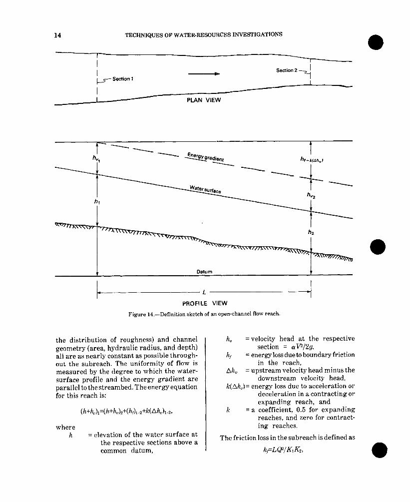
14 TECHNIQUES OF WATER-RESOURCES IlWE!3TIGATIONS
I I
c- Section 1
I I
--Y
-- Section 2 -I
--i PLAN VIE\N
-1 --- -r&l&
-- hf+klAh,l
h2
~--.----L----J PROFILE VIEW
Figure 14.-Definition sketch of an open-channel flow reach.
the distribution of roughness) and channel geometry (area, hydraulic radius, and depth) all are as nearly constant as possible through- out the subreach. The uniformity of flow is measured by the degree to which the water- surface profile and the energy gradient are parallel to the streambed. The energy equation for this reach is:
where h = elevation of the water surface at
the respective sections above a common datum,
h, = velocity head at the respective section = cuTn/2g,
hf = energy loss due to boundary friction in the reach,
Ah” = upstream velocity head minus the downstream velocity head,
k(.bh,)= energy loss due to acceleration or deceleration in a contracting or expanding reach, and
k = a coefficient, 0.5 for expanding reaches, and zero for contract- ing reaches.
The friction loss in the subreach is defined as
&WWG&,
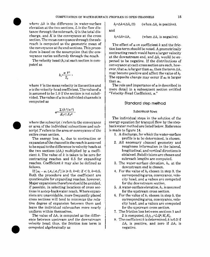
COMPUTATION OF WATER-SURFACE PROFILE23 IN OPEN CHANNELS 15
where Ah is the difference in water-surface elevation at the two sections, L is the flow dis- tance through the subreach, Q is the total dis- charge, and K is the conveyance at the cross section. The mean conveyance through the sub- reach is computed as the geometric mean of the conveyance at the end sections. This proce- dure is based on the assumption that the con- veyance varies uniformly through the reach.
The velocity head (h,) at each section is com- puted as
h,=a-2If , II
where Vis the mean velocity in the section and (Y is the velocity-head coefficient. The value of IX is assumed to be 1.0 if the section is not subdi- vided. The value of 01 in subdivided channels is computed as
where the subscript i refers to the conveyance or area of the individual subsections and sub- script T refers to the area or conveyance of the entire cross section.
The energy loss, h,, due to contraction or expansion of the channel in the reach is assumed to be equal to the difference in velocity heads at the two sections (Ah,) multiplied by a coeffi- cient k. The value of k is taken to be zero for contracting reaches and 0.5 for expanding reaches. Coefficient k may also be defined as follows.
If [a~ - (Y~ (AI/A,)~] is > 0, k=O; if < 0, k=0.5. Both the procedure and the coefficient are questionable for expanding reaches, however. Major expansions therefore should be avoided, if possible, in selecting locations of cross sec- tions in a step-backwater reach. Where expan- sions are unavoidable, more frequently placed cross sections will tend to minimize the rela- tive degree of expansion between them and leave the individual subreaches more nearly uniform within themselves.
The value of Ah, is computed as the differ- ence between upstream and the downstream velocitv head: thus. the friction loss term is a computed algebraically as
hf=Ah+(AhJ2) (when Ah, is positive),
and
hf=Ah+Ah, (when Ah, is negative).
The effect of (Y on coefficient k and the fric- tion loss term should be noted. A geometrically contracting reach would have a larger velocity at the downstream end, and Ah, would be ex- pected to be negative. If the distributions of conveyance at each cross section are such, how- ever, that (~1 is larger than (~2, then the term Ah, may become positive and affect the value of h,. The opposite change may occur if (~2 is larger than CY~.
The role and importance of (Y is described in more detail in a subsequent section entitled “Velocity-Head Coefficient, (Y.”
Standard step method
Subcritical flows
The individual steps in the solution of the energy equation for tranquil flow by the step- backwater method are listed below. Reference is made to figure 14.
1. A discharge, for which the water-surface profile is to be determined, is chosen.
2. All necessary channel geometry and roughness information in the lateral, longitudinal, and vertical directions is obtained. Subdivisions are chosen and subreach lengths are computed.
3. The water-surface elevation, h2, at the downstream end is chosen.
4. For the value of hz chosen in step 3, the corresponding area, conveyance, velo- city head, and (Y values are computed for the downstream section.
5. A water-surface elevation, hl, is assumed for the upstream cross section.
6. For the value of hl chosen in step 5, the corresponding area, conveyance, velo- city head, and [Y values are computed for the upstream cross section.
7. The friction loss between sections 1 and 2 is computed, (h&=L@/KlK2.
8. The coefficient k is determined; k is 0.5 if Ah, is positive, and zero if Ah, is negative.

16 TECHNIQUES OF WATER.-RESOURCES INVESTIGATIONS
9. The energy equation is solved. If the equation is acceptably balanced, the next operation is step 12.
10. If the energy equation is not balanced within an acceptable predetermined tolerance, a new value of hi is chosen for the upstream water-surface eleva- tion.
11. Steps 5 through 10 are repeated until the energy equation is satisfactorily balanced.
12. The solution moves one step, or sub- reach, farther upstream. The value of h! at the upstream end of the first sub- reach is now equivalent to the value of h2 at the downstream end of the new subreach. This operation is equivalent to step 3, above.
13. Steps 4-12 are repeated subreach by subreach until the water-surface pro- file throughout the entire reach has been computed.
If the first value of hz in step 3 for the most downstream cross section is above the normal- depth line, the profile computed will follow an Ml curve; if h2 is started originally at an eleva- tion below normal depth, the computed profile will follow an M2 curve. To determine the normal-depth line in a channel, the procedure is to choose two or more starting values of 1h at the most downstream cross section, and, for the same discharge, compute the resultant profiles until these profiles all converge farther upstream, and thereafter give identical values of water-surface elevation at succeeding cross sections. Limitations to this method of deter- mining convergence are discussed in the sec- tion entitled “Convergence of Backwater Curves.”
Because of the trial-and-error nature of the solution of the energy equation, manually deter- mining water-surface profiles is extremely tedious. Computer programs for the determi- nation of water-surface profiles by the step- backwater method are available for subcritical- flow conditions (Shearman, 1976).
Supercritical flows
For supercritical-flow conditions, the stand- ard step method of computing water-surface profiles, as described above for subcritical
applied similarly, but in a down- stream dire&ion. With reference to figure 14, the first step is to choose the upstream eleva- tioln, hl, and then to balance the energy equa- tioln by choosing an appropriate value of h2 for the downstream cross section. The solution progresses subreach by subreach in the direc- tion of the flow until the water-surface profile is determined throughout the entire length of reach in which the flow is supercritical. It is advantageous to choose the upstream elevation of the first subreach at critical depth, because generally, supercritical-flow computations would begin at a control point in natural chan- nels.
Much of the tediousness of a manual compu- tation olf a supercritical-flow water-surface profile is alleviated by partial use of an elec- tronic computer. Computer programs for sub- critical flow provide, as part of their output, ta.bles of cross-section properties at numerous elevations for all cross sections.in a reach. For each of the elevations, values of cross-sectional area, conveyance, velocity-head coefficient (QL), tolp width, stations at left and right edges of water, and wetted perimeter are given. If a sufficiently small elevation increment is speci- fied, it is a relatively easy matter to prepare plots or to interpolate directly from these com- puter tables, so that the appropriate values of area, colnveyance, and LY can be quickly deter- mined for any elevation. The trial-and-error procedure of balancing the energy equation is thus considerably simplified. Supercritical- flow conditions usually exist for only a few subreaches; therefore, the manual procedure described above should be used from a control point to a cross section downstream from it, at which a subcritical-flow profile solution has indicated the possibility of a hydraulic jump.
Field Data
All of the channel-geometry considerations that go into the selection of sites for slope-area a.nd n-verification measurements apply as well for each subreach of a step-backwater reach. Some of these are discussed in the following paragraphs, together with the special require- rnents Iof the step-backwater method.

COMPUTATION OF WATER-SURFACE PROFILES IN OPEN CHANNELS
A stadia survey Ol- equivalent stream channel is required for each study site. The surveys are run using the same basic techniques described by Benson and Dalrym- ple (1967) for indirect discharge measure- ments. A common datum must be established by levels throughout the length of the reach. Gage datum should be used in the vicinity of gaging stations.
Maps and ground elevations from photo- grammetric methods or from topographic maps with contours at close intervals are prac- tical alternatives to field surveys. Horizontal and vertical control points throughout the reach must be established.
Total reach length
Limiting total length of reach to be surveyed to the shortest useful distance is important in keeping costs of field surveys or photogram- metry reasonable. The length of reach needed to ensure convergence of computed backwater curves depends on the slope, the roughness, and the mean depth for the largest discharge for which the normal-depth profile is desired. Because the length depends on the depth, and the depth itself is the unknown which must ultimately be determined, the total reach length must be computed by estimating the normal depth.
Bresse’s equations (Woodward and Posey, 1941) for backwater curves may be used to determine the distances required for Ml and M2 backwater curves to converge to the nor- mal-depth profile. Figure 15 represents the equations in graphic form for steady, uniform, tranquil flow in a wide, rectangular channel, where the initial elevation of the M2 curve is 0.75 times the normal depth, and the initial elevation of the Ml curve is 1.25 times the nrmal depth. Profile convergence is accepted when the computed M2 depth is 0.97 times the normal depth, or the computed Ml depth is 1.03 times the normal depth.
The equations for the curves in figure 15 are:
L& y=O.86-0.64 F2 (M ,I
and
.I curve),
0.8
0.6
0 .I .2 .3 .4 .5 .6 .7 .8 .9 1.0
Figure 15.-Graphic determination of distances required for convergence of Ml and M2 backwater curves in rectangular channels.
L&l y- =0.57-0.79 F2 (M2 curve), ,I
where L is the required total reach length, So is the bed slope, yl, is the normal depth, and F is the Froude number.
After an estimate of the depth is made, the Froude number for the maximum discharge to be considered can be computed for a typical cross section. By entering figure 15 along the ordinate, where F2 is equal to @T/gA3, corres- ponding values of L&/y,, can be determined for either an Ml or an M2 curve. A mean bed- slope value is chosen for the reach, and the total convergence length is computed.
It is evident from figure 15 that an Ml curve that has started an equivalent distance above the normal depth (1.25 y,!), as compared to an M2 curve starting the same relative distance below the normal depth (0.75 y),), will require a much longer length of reach to converge to a comparable degree with the normal depth line.
An alternate estimate of the total length of reach required for an M2 backwater curve, starting at an elevation of about 0.75 y,,, to converge to within 3 percent of the normal- depth elevation (about 0.97 y,,), is given by the equation:
L,O.4 YH s,’

18 TECHNIQUES OF WATER-RESOU:RCES INVESTIGATIONS
where L, y,!, and So are defined as for figure 15. This equation is equivalent to a value of F2 of about 0.2 on the M2 curve of figure 15, or a value of F of about 0.45, which is representative of most natural flows.
Because channel roughness has a minor effect on the rate of convergence of computed backwater curves, n is neglected in these approximations of total length.
Locations of cross sections
In natural stream channels, cross sections are placed at intervals which will divide a total reach into a series of subreaches each of which is as uniform in geometry and roughness as practical. Dividing a reach is a relatively easy matter in slope-area and n-verification studies, where reaches are chosen for their conformity to ideal conditions. In profile computations through long stretches of a river, one must work with conditions as they are. Frequently they are far from ideal. Fairly uniform chan- nels will require fewer cross sections than those having many irregularities in size, shape, slope, or roughness. The cross sections should be representative of the reach between them and should have nearly the same characteris- tics. They should be located to enable proper evaluation of energy losses. With reference to figure 14, cross sections should be located at such intervals that the energy gradient, the water-surface slope, and the streambed slope are all as nearly parallel to each other as possi- ble and as close to being straight lines as possi- ble. If any channel feature causes one of these three profiles to curve, break, or run unparallel to the others locally, this is a clear indication that that particular subreach should be further subdivided. If cross sections are located accord- ing to the general criteria listed below, reason- able evaluations of energy losses can be made. Many of the criteria apply equally as well to slope-area and n-verification reaches. Cross sections:
1. Should be located at all major breaks in bed profile. If old flood profiles are available, cross sections should also be placed at major breaks in the known water-surface profile.
2. Should be placed at points of minimum and maximum cross-sectional areas.
3. Should be placed at shorter intervals in expanding reaches and in bends to minimize errors, because areas with upstream flow, dead water, or flow at an angle cannot be evaluated quantita- tively. To represent flow by the relation Q=K.W, it is necessary for the distri- bution of discharge across any section to be similar to the distribution of con- veyance in that cross section. In the computations, it is further assumed that all flow is downstream and per- pendicular to the cross sections. These assumptions are violated at expansions, embayments, and bends, where eddies or dead water may exist.
4. Should be placed at shorter intervals in reaches where the conveyance changes greatly as a result of changes in width, depth, or roughness. Because friction losses within subreaches are computed with a conveyance equal to the geo- metric mean of the end conveyances, the relation between upstream con- veyance, K,, and downstream convey- ance, K2, should satisfy the criterion: 0.7 < (KJK,) < 1.4. Conveyance, if it varies between cross sections, should do so at a uniform rate.
5. Should be located at points where rough- ness changes abruptly, for example, where the flood plain is heavily vege- tated or forested in one subreach, but has been cleared and cultivated by the land user at the adjacent subreach. In such an instance, the same cross sec- tion should be used twice, once as part of the rougher reach, and once again only a foot or two away, as part of the smoother reach. Because hsL@/KIK,, and L is extremely small, the effects of the error in h, are minimized. If flow from an upstream cross section with clear flood plains reaches a cross sec- tion where the overbanks are heavily vegetated, the condition is akin to a contracted opening. Similarly, if flow from an upstream cross section with heavily vegetated flood plains reaches a cross section where the flood plains

COMPUTATION OF WATER-SURFACE PROFILES IN OPEN CHANNELS 19
are clear and the roughness coefficient is relatively much smaller, the condi- tion is akin to expanding flow at the downstream end of a constriction. There are no adequate guidelines in these two situations for properly deter- mining friction losses, contraction losses, and expansion losses, nor for computing the water-surface profiles. The use of a cross section twice, in close proximity, and with different roughness values, must suffice for the present.
6. Should be placed between sections that change radically in shape, even if the two areas and the two conveyances are nearly the same. (Consider, for exam- ple, sections that change shape from just a main channel to a main channel with overbank flow, or from triangular to rectangular.)
7. Should be placed at shorter intervals in reaches where the lateral distribution of conveyance in a cross section changes radically from one end of the reach to the other, even though the total area, total conveyance, and cross-sectional shape do not change much. In general, the cross section having more subdivi- sions will have a larger (Y. A large value of (Y can have as much effect on the magnitude of a velocity head as can a change in cross-sectional area.
8. Should be placed at shorter intervals in streams of very low gradient which are significantly nonuniform, because the computations are very sensitive to the effects of local disturbances or irregularities. These effects can be reflected far upstream. Shorter sub- reaches may help to reduce these ef- fects. See the section entitled “Local Effects on Profiles.”
9. Should be located at and near control sections, and at shorter intervals im- mediately downstream from control sections, if supercritical-flow condi- tions exist.
10. Should be located at tributaries that contribute significantly to the main stem. The cross sections should be placed such that the tributary would
enter the main stem in the middle of a subreach.
11. Should be located at bridges in the same locations as required for computations of discharge at width constrictions(see Matthai, 1967):
(a) just downstream of the bridge, across the entire valley,
(b) at the downstream end of the bridge, within the constric- tion,
(c) at the approach cross section, one bridge-opening width upstream,
(d) if there is road overflow, along the higher of either the crown or curb, including the road approaches to the bridge, and the bridge deck.
It would seem, from a perusal of the list of suggested cross-section locations above, that the effects of almost all the undesirable features of nonuniform, natural stream channels can be lessened by taking more cross sections. This is true, but consideration must also be given to the time, cost, and effort to locate and survey additional cross sections. A balance must be set between the number of cross sections deemed desirable, and the number that is practical. These criteria for cross-section loca- tions serve, therefore, to call attention to the considerations behind the need for cross sec- tions, and. to help the engineer to understand anomalies in computed profiles if cross sec- tions are omitted. Practice will provide the engineer with the experience necessary to anticipate the circumstances that would per- mit relaxation of, or elimination of, some of these criteria, and the probable nature and magnitude of resultant errors.
Individual subreach lengths
In addition to the criteria for locations of cross sections, there are a few considerations as to reach lengths and number of subreaches which will influence the selection of cross sections:
1. The total reach length should be divided into at least lo-12 subreaches to be rea- sonably sure of convergence.

20 .-
TECHNIQUES OF WATER-RESOURCES INVESTIGATIONS >i
2. No subreach should be longer than about 75-100 times the mean depth for the largest discharge to be considered, or about twice the width of the subreach: This is a maximum limit, and applies only if other considerations for cross- section locations do not control.
3. The fall in a subreach should be equal to or greater than the larger of 0.50 foot, or the velocity head, unless bed slope is so flat as to require defaulting to the second criterion in this list.
4. The subreach length should be equal to or less than the downstream depth (for the smallest discharge to be considered) divided by the bed slope.
Profile computations for a range of dis- charges may require one set of subreach lengths for all discharges within banks and another set o:f subreach lengths for discharges with pver- bank flow. Extra cross sections may be neces- sary within the main channel for the lower discharges to satisfy some of the criteria listed in the section entitled “Locations of Cross Sections.”
Cross-section attributes
5. If the bed profile is a convex or concave curve, the reach should be broken up into shorter subreaches, because the losses within the reach might not be properly accounted for. In this method of computation, straight-line variation of bed elevations between end cross sec- tions is assumed.
Up to 200 points may be used to define the shape of each cross section in the U.S. Geologi- cal Survey’s computer solution (Shearman, 1976). Data for each point are a ground eleva- tion and a transverse station number (distance from a ref’erence point on the left bank) which increases in magnitude toward the right bank. At woss sections that start with negative sta- tion numbers, the stationing would be less negative toward the right bank. The ends of the cross section must be extended higher than the expected water-surface elevation of the largest flood that is to be considered in the subreach.
Weighted length of a subreach All cross sections must be perpendicular to
If water-surface profiles for several dis- charges are to be computed, the lengths be- tween any two cross sections may have to be computed differently for different discharges. Small discharges would stay entirely within banks and follow the meanders of the main channel. The length for the subreach would be a maximum. Large discharges may have flood- plain flows, and their effective flow distances would be shorter.
the flow direction throughout the entire width of the cross section. If the flow pattern warrants a broken, or dog-legged cross section, each subsection of the cross section should be per- pendicular to the direction of flow through that subsection. All subsections of a cross sec- tion should be straight lines.
For overbank flows, a weighted or effective subreach length must be used. The centroids of conveyance in the subsections of each cross section are determined and connected through the subreach by curvilinear or straight lines. One line will follow the main channel, and the others will be along the flood plains. The length of the main channel is multiplied by the con- veyance for the main channel, and the lengths along the flood plain are multiplied by the cor- responding overbank conveyances. The sum of these products is divided by the total convey- ance to obtain the weighted subreach length.
Cross sections should not cross each other within the live-flow boundaries of the channel, nor should they ever be drawn so as to share a common subsection on one end. There must be a measurable longitudinal distance between each subsection of one cross section, and a cor- responding subsection of the adjacent cross sections, upstream and downstream.
Cross sections at. bridges and at road-over- flows are described in detail in the section entitled “Bridges.”
Subdvisions of cross sections
Criteria for subdividing cross sections are the same as those described by Benson and Dalrymple (1967) for indirect measurements

COMPUTATION OF WATER-SURFACE PROFILES IN OPEN CHANNELS 21
of discharge. Subdivision should be done marily for major breaks in cross-sectional geometry. Besides these, major changes in roughness may call for additional subdivi- sions. The roughness coefficients verified by the Geological Survey (Barnes, 1967) are based on unit cross sections that have complete or nearly complete wetted perimeters. Basic shapes that are approximately rectangular, trapezoidal, semicircular, or triangular are unit sections having complete wetted perime- ters. Subdivisions for major breaks in geometry or for major changes in roughness should, therefore, maintain these approximate basic shapes so that the distribution of flow or con- veyance is nearly uniform in a subsection.
The importance of proper subdivision, as well as the effects of improper subdivision, can be illustrated very dramatically. In figure 16, a trapezoidal cross section having heavy brush and trees on the banks has been subdivided near the bottom of each bank because of the abrupt change of roughness there. A large percentage of the wetted perimeters(P) of the triangular subareas (AI and As) and possibly of the main channel (AZ) is eliminated. A smaller wetted perimeter abnormally increases the hydraulic radius (R=A/P), and this in turn results in a computed conveyance different from the conveyance determined for a section with a complete wetted perimeter. In figure 16, a conveyance (KT) has been computed for the cross section that would require a compo- site n value of 0.034. This is less than the ‘12 values of 0.035 and 0.10 that describe the roughness for the various parts of the basic trapezoidal shape. The basic shape should be left unsubdivided, and an effective value of n somewhat higher than 0.035 should be assigned to this cross section, to account for the addi- tional drag imposed by the larger roughness on the banks.
At the other extreme, the panhandle section in figure 17, having a main channel and an overflow plain, must be subdivided into two parts having nearly complete wetted perime- ters. The value of n is 0.040 throughout the section. If the section is not subdivided, the increase in wetted perimeter of the flood plain is relatively large with respect to the increase in area. The hydraulic radius is abnormally reduced, therefore, and a fictitious, lower value
of 0.028 for n is needed to obtain the conveyance equivalent to that of a unit section. It is clear that irregular cross sections such as that in figure 17 should be subdivided to create indi- vidual basic shapes.
The cross section shapes in figures 16 and 17 represent two extremes of the problems asso- ciated with improper subdivision. Between these two are shapes with benches or terraces, as shown at the top of figure 18. R. H. Tice, 1973, “Subdivision and the Hydraulic Radius Term in Flood-Flow Formulas:“(written com- munication) has suggested criteria which are generally quite satisfactory for subdivision of bench panhandle shapes. He recommends sub- division if the value of the ratio L/y is 5 or greater (see figure 18). He also recommends subdivision of a large, flat triangular shape with a central angle of 150” or more, because L/y would be about 5 or greater. If the value of L/y is almost 5, he recommends that the subdi- vision be made at a distance of about L/4 from the edge of water. For L/y equal to 20 or greater, Tice recommends several subdivisions. For very large values of L/y, the cross-sectional slope would become flatter, the depth would become more uniform, and, consequently, the distribution of velocities would be more uni- form; no subdivisions would be required on the basis of shape alone, but subdivisions on the basis of roughness distribution would be permissible.
Another shape criterion for subdivision has been proposed by Matthai (oral communica- tion, 1973) and is shown in figure 19. If the main-channel depth is more than twice the depth at the stream edge of the overbank area, Matthai recommends subdivision.
Subdivision on the basis of geometry should be coordinated with the expected range in depths. For example, the cross section of fig- ure 20 should be subdivided differently for different stages, as shown in the figure.
There are borderline cases in which the decision to subdivide could go either way. Subdivisions in adjacent sections should be similar to avoid large differences in CL There- fore, if a borderline case is between sections that do not require subdivision, do not subdi- vide; if between sections that must be subdi- vided, subdivide the borderline case. Where the section in question is between one that

22 TECHNIQUES OF WATER-RESOURCES INVESTIGATIONS
Subarea 1 Subarea 2
-I_
A, =A3=50 AZ= 500 P,=P3=14.14 Pz= 50 R, = R3=3.54 Rz= 10 K,=K3=1730 K2=98,500
KT=K,+K2+K3
= 102,000
Compositesolution: A,=600 PC= 78.3 I?,= 7.66
” = ‘.-w”=o 034 c KT
Figure 16.-Effects of subdivision on a trapezoidal section.
must be subdivided and one that should not be subdivided, proceed so that the sections are the best representation of a uniform reach.
Besides the shape and roughness criteria for subdivision described here, the step-backwater computer program used by the Geological Survey requires additional subdivision points.
One example of computer-required subdivi- sion of cross sections is associated with the Froude number test limit. The Froude number, as defined in the section on “Locus of Critical- Depth Stages,” is expressed by the equation
6 Q/A *=l/zmm '
in which the value of LY is frequently close enough to unity to be ignored. The Froude number does not directly enter computations in the step-backwater method: instead, it serves as a mechanism to warn of the possibility of supercritical-flow conditions. The Froude num-
ber for a cross section with relatively shallow overflow is not a reasonable index of either subcritical or supercritical flow. It is a reason- able index for aunit section such as a trapezoid- al main (channel. The Froude number for the main channel is considered a more reasonable index of flow conditions than Froude numbers for over:bank subsections. Therefore, a cross section with overbank flow should be subdi- vided so that the main-channel subsection will have the largest conveyance throughout the range of water-surface elevations expected. To be certain that this relation holds, extra subdi- visions may be necessary on wide overbank areas or those having very low roughness coef- ficients. Then the index Froude number for th,e main channel can be computed from the equation:
E’RDN= Qr KL
K,A,m’

COMPUTATION OF WATER-SURFACE PROFILES IN OPEN CHANNELS 23
1 Ift I
t loft
1
Subarea 1
n=0.040
Subarea 2
(Not drawn to scale)
lOOft- L
A,= 100 AZ= 670.5 P,’ 101 Pz= 79.7 R,= 0.990 R2= 8.41 K,=3700 K2=103,000
KT= K, + K2
= 107,000
Compositesolution: A,=770.5 P,=108.7 R,= 4.26
n = 1.466MPz0 028 c
KT
Figure 17.-Effects of subdivision on a panhandle section.
Subscripts T and L designate values for the total cross section and the subsection having the largest conveyance, respectively.
Other subdivisions are required where there are bridges within the reach. Approach cross sections at bridges should be subdivided on the basis of the location of the K,, subsection (Mat- thai, 1967) in addition to all the other consid- erations mentioned above.
The Geological Survey computer program provides for up to 20 subdivisions per cross section. As many of these should be used as necessary to adequately define (Y for the cross section.
Figure 21 illustrates the criteria for subdi- vision of an approach cross section at a bridge. The solid lines represent subdivision on the
basis of shape or roughness. In addition, the left overbank is subdivided (dashed line) to ensure that the subsection with the largest conveyance will be the main channel. Within the main channel section, another two subsec- tions are created by the limits of the K,, subsec- tion, representing the upstream projection of the boundaries of the constriction.
Velocity-head coefficient, 01
Effects of the velocity-head coefficient have been mentioned in the discussion of figure 14 and the energy equation. It is important to understand the role of (Y and the method of computing it in open-channel flow computa- tions.
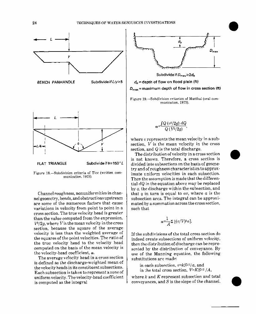
24 TECHNIQUES OF WATER-RESOURCES INVESTIGATIONS
BENCH PANHANDLE Subdivide if Uyr5
FLAT TRIANGLE Subdivideiftk150”L
Figure l&--Subdivision criteria of Tice (written com- munication, 1973).
Channel roughness, nonuniformities in chan- nel geometry, bends, and obstructions upstream are some of the numerous factors that cause variations in velocity from point to point in a cross section. The true velocity head is greater than the value computed from the expression, v2/2g, where Vis the mean velocity in the cross section, because the square of the average velocity is less than the weighted average of the squares of the point velocities. The ratio of the true velocity head to the velocity head computed on the basis of the mean velocity is the velocity-head coefficient, (Y.
The average velocity head in a cross section is defined as the discharge-weighted mean of thevelocity heads in its constituent subsections. Each subsection is taken to represent a zone of uniform velocity. The velocity-head coefficient is computed as the integral
Subdivide if Dmaxz2db
db = depth of flow on flood plain (ft)
D m,8X= maximum depth of flow in cross section (ft)
Figure 19.4ubdivision criterion of Matthai (oral com- munication, 1973).
azSQ (v2/2d dQ Q (W2.d '
where v represents the mean velocity in a sub- section, V is the mean velocity in the cross section, and Q is the total discharge.
The distribution of velocity in a cross section is not known. Therefore, a cross section is divided into subsections on the basis of geome- try and (of roughness characteristics to approx- innate uniform velocities in each subsection. Then the assumption is made that the differen- tial dQ in the equation above may be replaced by 4, the discharge within the subsection, and that 4 in turn is equal to av, where a is the subsection area. The integral can be approxi- mated by a summation across the cross section, such th,at
a=+ [(vlvyal. If the subdivisions of the total cross section do indeed create subsections of uniform velocity, then the distribution of discharge can be repre- sented by the distribution of conveyance. By use of the Manning equation, the following substitutions are made:
in each subsection, v=kW/a, and in the total cross section, V=KSI2 /A,
where k and K represent subsection and total conveyances, and S is the slope of the channel.

COMPUTATION OF WATER-SURFACE PROFILES IN OPEN CHANNELS 25
1C
C .,
8
7
ii f 6
z .
g E
P !Y 4 Lu
3
2
1
C
I-
i-
i-
I-
, _
1
‘,
I
10 20 30 40
STATION, IN FEET
Range of water-surface
Substation
elevation, in feet Station 20 Station 10 o-2 No - 2-4 Yes - 4-6 No -
6-8 No Yes 8-10 No No
Figure ZO.--Cross section in which subdivision could be dependent on expected elevations of water surface.
The latter is assumed to be identical in each subsection. The expression for the velocity-head coefficient thus reduces to the familiar form,
In general, the more subdivisions in a cross section, the larger (Y will become. Because of the effect (Y has in the velocity-head term, (~v2/29, the cross section should be subdivided, as needed, to validate as nearly as possible the assumptions mentioned.

26 TECHNIQUES OF WATER-RESOUFCCES INVESTIGATIONS
Figure 21.~Subdivision of an approa.ch cros:; section at a bridge.
In manual computations, it is possible to account for dead water or negative flows in parts of a cross section by assigning values of zero or of negative numbers for the subsection conveyances. Coefficient LY will, therefore, be properly computed. In machine computations, however, it is not easy to assign zero or nega- tive values because of the implicit understand- ing that conveyance and discharge are sim- ilarly distributed across a cross section. This implicit understanding is particularly impor- tant at bends, embayments, and expansions, and at cross sections downstream from natural and manmade constrictions. If dead water or upstream flow is suspected, subdivisions should isolate these parts. Then, by omitting the sub- sections or assigning very large n’s to them, a better (Y will be computed.
Instances have been reported of values of (Y in excess of 20, with no satisfactory explana- tions for the enormous magnitude of the coeffi- cient. If adjacent cross sections have compara- ble values, or if the changes are not sudden between cross sections, such values can be accepted, but if the change is sudden, some attempt should be made to obtain uniformity. This could be clone with more cross sections to achieve gradual change, or it can be done by resubdividing the cross section. Some subsec-
tions can be consolidated (as long as the main- channel subsection remains the largest one), but compensation should probably be made for the fewer subdivisions, possibly by increasing the roughness coefficients somewhat or by decreasing areas somewhat.
Roughness coefficients
Criteria for the selection of roughness coef- ficients for indirect discharge measurements are described in detail by Benson and Dal- rymple (1967), and they all apply equally well to computations of water-surface profiles by the step-backwater method. In addition to these, B’arnes (1967) provides color photographs and details of channel geometry for many slope- area reaches in which values of n, the roughness c’oefficient, were verified.
The Survey’s computer program has provi- sion for varying n with depth. (The depths referred to in this paragraph are mean hy- draulic depths.) For each subsection, two key mean depths may be selected, with a value of n for each. At all flows for which the mean depth corresponding to the water-surface elevation is equal to or less than the lower key mean depth, the subsection roughness coefficient
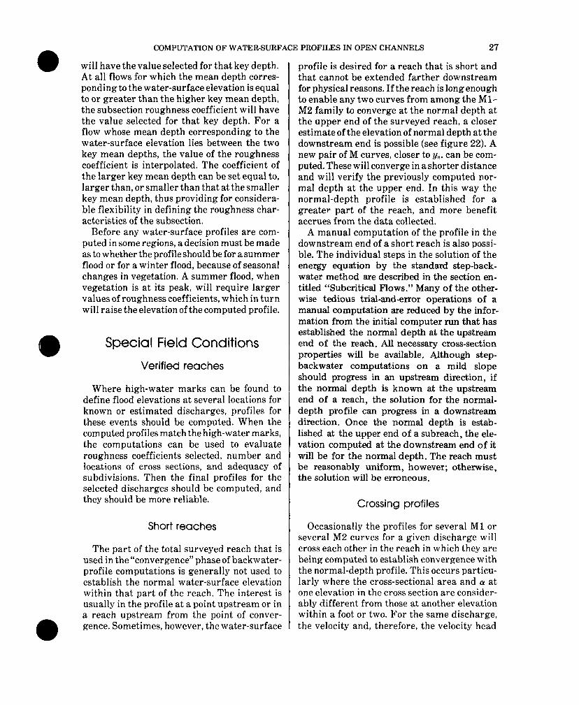
COMPUTATION OF WATER-SURFACE PROFILES IN OPEN CHANNELS 27
will have the value selected for that key depth. At all flows for which the mean depth corres- ponding to the water-surface elevation is equal to or greater than the higher key mean depth, the subsection roughness coefficient will have the value selected for that key depth. For a flow whose mean depth corresponding to the water-surface elevation lies between the two key mean depths, the value of the roughness coefficient is interpolated. The coefficient of the larger key mean depth can be set equal to, larger than, or smaller than that at the smaller key mean depth, thus providing for considera- ble flexibility in defining the roughness char- acteristics of the subsection.
Before any water-surface profiles are com- puted in some regions, a decision must be made as to whether the profile should be for a summer flood or for a winter flood, because of seasonal changes in vegetation. A summer flood, when vegetation is at its peak, will require larger values of roughness coefficients, which in turn will raise the elevation of the computed profile.
Special Field Conditions
Verified reaches
Where high-water marks can be found to define flood elevations at several locations for known or estimated discharges, profiles for these events should be computed. When the computed profiles match the high-water marks, the computations can be used to evaluate roughness coefficients selected, number and locations of cross sections, and adequacy of subdivisions. Then the final profiles for the selected discharges should be computed, and they should be more reliable.
Short reaches
The part of the total surveyed reach that is used in the “convergence” phase of backwater- profile computations is generally not used to establish the normal water-surface elevation within that part of the reach. The interest is usually in the profile at a point upstream or in a reach upstream from the point of conver- gence. Sometimes, however, the water-surface
profile is desired for a reach that is short and that cannot be extended farther downstream for physical reasons. If the reach is long enough to enable any two curves from among the Ml- M2 family to converge at the normal depth at the upper end of the surveyed reach, a closer estimate of the elevation of normal depth at the downstream end is possible (see figure 22). A new pair of M curves, closer toy,,, can be com- puted. These will converge in a shorter distance and will verify the previously computed nor- mal depth at the upper end. In this way the normal-depth profile is established for a greater part of the reach, and more benefit accrues from the data collected.
A manual computation of the profile in the downstream end of a short reach is also possi- ble. The individual steps in the solution of the energy equation by the standard step-back- water method are described in the section en- titled “Subcritical Flows.” Many of the other- wise tedious trial-and-error operations of a manual computation are reduced by the infor- mation from the initial computer run that has established the normal depth at the upstream end of the reach. All necessary cross-section properties will be available. Although step- backwater computations on a mild slope should progress in an upstream direction, if the normal depth is known at the upstream end of a reach, the solution for the normal- depth profile can progress in a downstream direction. Once the normal depth is estab- lished at the upper end of a subreach, the ele- vation computed at the downstream end of it will be for the normal depth. The reach must be reasonably uniform, however; otherwise, the solution will be erroneous.
Crossing profiles
Occasionally the profiles for several Ml or several M2 curves for a given discharge will cross each other in the reach in which they are being computed to establish convergence with the normal-depth profile. This occurs particu- larly where the cross-sectional area and CY at one elevation in the cross section are consider- ably different from those at another elevation within a foot or two. For the same discharge, the velocity and, therefore, the velocity head

28 TECHNIQUES OF WATER-RESOURCES INVESTIGATIONS
Second sat of M, CUN~~
~lrstset of M2cutv~~
Figure 22.-Establishment of the normal-depth profile in a short reach.
may be sufficiently higher for the lower of two profiles such that the water-surface elevation computed for the next section upstream will be higher for what was the lower profile than for what was the higher profile.
Profiles will also cross in the first subreach if the starting elevation for one profile is less than the elevation of critical depth at the first cross section and the other starting elevation is above the critical-depth line. Because there is no Froude number check at the first cross sec- tion, care must be taken to ensure that starting elevations for M2 profiles are never below the critical-depth line,
Profiles can cross elsewhere in a reach if the Froude number limit is set so high as to accept otherwise super-critical solutions. Solutions in- volving Froude numbers larger than 1.5 should not be accepted, and computed profiles for any reaches with Froude numbers unity should be closely examined.
larger than
Profiles that cross need not be more than a disconcerting problem if they occur in a steeply sloped stream, or if they occur on any M2 curves near the elevation of critical depth, where the M2 curve itself is naturally steep. Ordinarily, on steep bed slopes or on steep parts of M2 curves, the phenomenon shows up as a loca1 perturbation that is quickly “righted” within a few subreaches. On flat slopes, however, the effects of such crossed profiles could extend far upstream. Unless crossed profiles either
quickly converge or recross to their original relative positions, such a solution should be examined closely.
Transitions between inbank and overbank flow conditions
Solutions of water-surface profiles are rather straightforward either if the flow is confined to the main channel throughout the reach or if flow is a combination of main-channel and overbank flow throughout the reach. If flow conditions change from one of these to the other, there could be an interruption of the solution or an anomaly in computed values. Recognition of the circumstances under which these problems occur is essential to the proper handlingor interpretationofthecomputations.
When flow breaks out over the banks or returns to t.he main channel between two cross sections, the very small change in elevation is associated with comparatively small changes in cross-sectional area and conveyance. There is a sudden change, however, in cross-sectional shape and in velocity-head coefficient, (r. If there is asudden, otherwise inexplicable jump in computed elevations both in manual and in machine computations, an abrupt change in (Y between the two cross sections may be the cause. a

COMPUTATION OF WATER-SURFACE PROFILES IN OPEN CHANNELS 29
A sudden change in cross sectional shape might not create difficulties in manual compu- tations of water-surface profiles. In machine computations, however, the solution might abort because of a Froude number problem. The explanation is that one of the overbank subsections may be larger in conveyance than the main-channel subsection; therefore, the Froude number is for the shallower depths of the overbank subsection.
If overbank subsections are further subdi- vided to avoid a Froude number problem, the increased number of subsections will increase the magnitude of the differences in (Y and the velocity-head term, cyV/29. This will in turn create or compound the problem of a sudden, unreasonable change in computed water-sur- face elevations. On the other hand, a reduction in the amount of subdivision (and cy) might induce the Froude-number problem.
Additional cross sections in the vicinity of the transition would improve the profile, but such a costly step might not be the ideal solu- tion nor would it wholly solve the problem. Additional cross sections might be satisfactory for one discharge, but higher or lower dis- charges will simply translate the same prob- lem to other points in the reach.
Either or both of the following methods should give satisfactory results for the deter- mination of water-surface profiles in the region of transition: A. Method of interrupting the computed
profile. 1. If the flow in the downstream reach is
within the banks (over the banks) and if in the upstream reach it is overbanks (within the banks), stop the computa- tion at the last cross section at which the flow is still inbank (overbank).
2. Project the computed water-surface profile upstream to the next cross sec- tion where flow is out of banks (within banks) on the bases of the computed profile up to the downstream cross section and the local geometry and bed slope.
3. Start a new profile computation at this upstream cross section, using the pro- jected water-surface elevation in step 2 as the starting elevation.
B. Method of averaging computed profiles. 1. Compute the water-surface profile for a
discharge larger than the one under consideration so that the flow will be overbank throughout the transition reach.
2. Compute the water-surface profile for a discharge smaller than the one under consideration so that the flow will be completely within banks in the transi- tion reach.
3. Estimate the profile for the given dis- charge through the transition reach from the profiles of steps 1 and 2.
Additional complications and uncertainties further compound the problem of sudden transitions between inbank and overbank con- ditions. These result from a lack of experience. For example, the sudden expansion of flow onto the flood plain from a completely inbank- flow situation is associated with tremendous expansion losses for which normally used com- putation guidelines may be inadequate; only 50 percent loss of energy is accounted for in an expanding reach. Conversely, the sudden drainage of overbank flows back into the main channel could be likened to a contracted open- ing-one for which present methods, and coef- ficients of contraction or of discharge for bridges, would not quite be applicable.
Flow at tributaries
As the computation of water-surface eleva- tions progresses along the stream channel, the discharge must be known at each cross section so that the appropriate velocity heads and fric- tion losses can be properly evaluated. At the mouth of a tributary, therefore, three dis- charges must be known:
1. Q,,, the main stem discharge, upstream from the confluence,
2. Qt, the discharge in the tributary, and 3. Qr(, the main stem discharge, downstream
from the confluence (sum of Q, and QJ. The main stem discharge, Qd, will be the one used up to the confluence. To continue the computations above the tributary, Q, must be known. Unless the tributary discharge, Qt, is known, some estimate of it must be made. Tice

30 TECHNIQUES OF WATER-RESOURCES IiWESTIGATIONS
(oral,commnnication, 1973) suggests the fol- lowing approximation in the absence of a more reliable value:
where At is the drainage area of the tributary at its mouth, and Ad is the drainage area of the main stem just below the tributary mouth.
It is implicit that the arrivals of the peaks of discharges Q, and Qf at the confluence are simultaneous for the frequency of the main- stem discharge, Qa. That is to say, the value of the loo-year discharge in the tributary should not necessarily be subtracted directly from the loo-year discharge on the main stem down- stream from the confluence in order to cleter- mine the loo-year discharge on the main stem upstream. The engineer must adjust the dis- charges Q,, and Qf for any significant lag time between the peaks along those channels.
When the discharges at the confluence are determined, the values of velocity heads and channel friction loss for the subreach into which the tributary flows, are computed as follows:
downstream velocity head = ad(Q~/A#/Zg, upstream velocity head = ~,(Q~,IAdWs~ and
friction loss, hf
where subscripts d and u denote downstream and upstream cross sections, L is the subreach length, and K is conveyance.
Because of the averaging of discharges, where QI, applies more nearly to the upstream part of the subreach, and Qd applies to the downstream part, the cross sections should preferably be located at points equidistant from the tributary. The larger the tributary is, the more likely it is that K,, and Kd will be appreciably different, thus violating the cri- terion for proper evaluation of friction losses, 0.7 <(K,,/Kd) < 1.4. Therefore, keep subreaches involving relatively large tributaries as short as practical, thereby confining uncertainties to the immediate locality.
The special case of a tributary in the imme- diate vicinity of a bridge is discussed in the section entitled “Bridges.”
Flow past islands
If the channel in which water-surface pro- files are being computed has an island so large that the paths around it are considerably dif- ferent in length, slope, and roughness charac- teristics, each path around the island must be h:andled as a separate reach. For example, in figure 23, the total discharge, Qf, is split into two unknown components, QL and QR. The computation progressing upstream has stopped at cross section A, at the downstream end of the isIand. The water-surface elevation at cross section U, just upstream of the island, must be computed to continue the profiles farther up- stream. The problem is complicated because the division of the flow into components QL and QR is not known.
The junctions of the separate channels are considered to be similar to tributaries; and cross sections A, BL, BR, FR, KL, and U are located as described in the section entitled “IFlow at Tributaries.”
Each channel around the island is analyzed by establishing a stage-discharge relation for cross section U. For example, by beginning with cross section A, and working up the left channel, the water-surface profiles for various discharges, QL, are computed up to section U. To begin with, QL may be assumed to be equal to Qr, and the water surface at U is computed. The same thing is done for several lower dis- charges, down to the other extreme, QL assumed tlo be zero. The stage-discharge relation is plot- ted as in figure 24 with water-surface elevation at U as ordinate, and QL as abscissa. A similar relation is plotted for the right channel as in figure 24. The intersection of the two curves determines the proper division of Qr into com- ponents QR and QL, and it indicates the eleva- tion of the water surface at cross section U. The computations would resume at cross section 1;’ with the starting elevation as determined from figure 24, and with the discharge, Qr. The intersection of the two rating curves of figure

COMPUTATION OF WATER-SURFACE PROFILES IN OPEN CHANNELS
Figure 23.-Flow around an island.
‘24 may be defined with more precision by defining the curves with more trial runs in that vicinity.
If a known quantity of flow, QB, bypasses the main channel and later returns to it, the solu-
l tion is greatly simplified because the division of discharge is known. There is no need to stop
the computation below the point where QB returns to the main channel. Water-surface profile computations would progress up the main channel without interruption as follows: up to cross section A, the discharge QT would be used; discharge would change to (&T-&B) at cross section BE, and remain so up through

32 TECHNIQUES OF WATER-RESOURCES INVESTIGATIONS
&(RIGHT CHANNEL),IN CUBIC FEET PER SECOND
,Q (LEFT CHANNEL), IN CUBIC FEET PER SECOND
Figure 24.-Division of flow around an island.
cross section FE; discharge would change to QT at cross section U, and remain so farther upstream.
Multichannel flows
If the main-channel flow is divided into sev- eral branches rather than only two, as de- scribed for flow around an island, the following procedures are recommended. They will help to determine the discharge through each chan- nel and the water-surface elevation upstream from the branches. The method is based on that described by Woodward and Posey (1941).
The main-channel cross section, D-D, in figure 25A, is the last for which a water-surface elevation has been computed with the total discharge, QT. The elevation at the upstream cross section, U-U,, must be determined as well as the division of QT into components QL, QM, QR, and any other branches, and the water- surface profiles in each branch.
To solve for the unknowns, an approximate division of flow is estimated, and each channel is analyzed by computing the profile for that
channel’s discharge from cross section D-D up to cross section U-U. In figure 258 the eleva- tion at U-U is plotted as ordinate, and the discharge producing it is plotted as abscissa. The steps are repeated for other estimated div- isions of flow until a rating curve is defined for stage at section U-U corresponding to dis- charge in each channel. An additional rating curve i:s drawn to represent total discharge as abscissa by adding, for several elevations, the quantities QL, Q,M , and QR. This final curve gives the relation between total discharge and elevatilon at the upstream cross section, U-U. The known value of Qr is used with figure 25B to determine the corresponding value of water- surface elevation at cross section U-U. The discharge in each branch for that elevation of U-U is determined from the individual branch rating curves. These discharges, QL, QM, and QR, ar,e now used to compute water-surface elevations in each channel between cross sec- tions L)-D and U-U.
In the computations of profiles from section D-D to section U-U through any one of the branches, there will be a sudden and large change in magnitude of conveyance (a) between

COMPUTATION OF WATER-SURFACE PROFILES IN OPEN CHANNELS
I I
QT
D I DM,& DR
I I
u
t t t QM QM QR
I
U&JR U&JR ut7
t t
QT QT
A,PLAN VIEW OF MULTICHANNEL FLOW
ii k! - z 5
p u+ z _
g- a u _
t _
E -
>Q - Y QL+QM+QR=QT I Lu I I I I I I I
0 QT
DISCHARGE,IN CUBIC FEET PER SECOND
B, RATINGS FOR INDIVIDUAL CHANNELS
Figure 25.-Division of flow in multichannel reach.
33

34 TECHNIQUES OF WATER-RESOURCES INVESTIGATIONS
section D-D and the first cross section in the branch, and (b) between the last cross section in the branch and section U-U. To minimize errors in the computation of head losses which are due both to expansion and contraction, and to channel friction, a logical and consistent method of subdividing sections D-D and U-U must be used. Three possible methods are:
1. The shapes of sections D-D and U-U, as determined from plots of those cross sections, may reveal some obvious geo- metric basis for subdivision. If so, arti- ficially extend these boundaries to the upstream and downstream ends of the islands or embankments, thereby div- iding the stream into channels.
2. On the basis of the water surface at section D-D, make a reasonable estimate of the water surface at section U-U. For these elevations, plot the cumulative convey- ance versus distance from left bank for sections D-D and U-U. The total con- veyances are labeled KD and &. Com- pute conveyances, KL, KM, and K,+ based on water-surface elevation at section D-D for the minimum cross section in each channel. Compute positions for pseudo-boundaries in sections D-D and U-U to simulate the actual boundaries of each branch by multiplying Ku and Ku by the ratio KJKL + KM + KR) for the division between the left and middle channels, and by (KL + KM)/(KL + KM + Kd for the division between the middle and right channels. Extend pseudo-boun- daries to the upstream and downstream ends of the islands or embankments.
3. On the basis of the water-surface elevation at section D-D, determine the gross cross-sectional areas for the most con- stricted cross section in each channel. Project the gross width of each island or embankment to the upstream end and divide it on the basis of these gross areas in the adjacent channels, as is illustrated in figure 29. This pseudo- boundary between channels is projected upstream to section U-U, and down- stream to section D-D, as is shown in figure 25A.
by the first two methods might not yield similar 0 divisions of section D-D and U-U, or they might be neither parallel to each other nor to extensions of the general axes of the dividing islands. The third method, which is suggested for multiple bridges, is least ambiguous, and shlould be used if there is not good reason to fa,vor one of the other methods.
After QLY QM, and QR are determined, and thle wat.er-surface elevation at U-U is com- puted, the velocities at U-Ushould be checked to’ make certain that they are subcritical. If the main-channel flow at U-U is not tranquil, the proportion of flow going into each channel will depend upon flow conditions upstream from the point of division.
If the flow in anyone channel is not tranquil, the steps described in the sections entitled “Steep !SIopes,” and “Supercritical Flows” are followed. The rating curve, as shown in Figure 2!SB for each channel, can still be defined in terms of discharge and the elevation at U-U.
Any one or all of the individual waterways of figure 25B could be natural stream channels around islands, bypass canals, or control struc- tures such as bridges, culverts, or dams. Indeed, e:ach path itself could have a series of such structures and(or) stretches of natural stream channel between cross sections U-U and D-D. The methods of computing water-surface ele- vations at bridges and at culverts are de- scribed in the appropriately entitled sections in this manual. Regardless of whether the flow t’hrough any one of the individual channels in figure 25B is subcritical or supercritical, or even whet,her the flow regime successively changes between sections U-U and D-D, the final relation to be plotted is between the dis- charge and the water-surface elevation at sec- tion U--U for each path.
Bridges
Some engineering judgment must be used to select the best method. Boundaries determined
Water-surface profile computations may be carried through bridges and other constric- tions providing that tranquil open-channel flow conditions exist and that no pressure flow is involved for the discharges being considered.
The effects of bridges or other constrictions on the computed Ml and M2 backwater curves
’

Effects on Profiles.” Bridges do not present a serious problem if they are located in the reach downstream from the point of convergence of Ml or M2 curves. Bridges located in a channel for which the water-surface profile is being computed, also present no serious problems if the amounts of backwater are insignificant compared to the total fall in the approach reach. This would be true in a streambed hav- ing a fairly good slope and at sites where there is not much contraction involved.
The computation of water-surface profiles at bridges, including bridges with road over- flow, has been incorporated into a computer program (Shearman, 1976). The methodology and coefficients outlined by the Bureau of Pub- lic Roads (Bradley, 1960, 1970) are used. Be- cause of the methodology within the program and by Bradley, the computer solution is satis- factory only for the circumstances described in the preceding paragraph. At other bridges computer solutions should be stopped and backwater curves should be manually com- puted. Manual computations should be consid- ered, in particular, at the following sites:
1. reaches having extremely flat streambed slopes,
2. two or more bridges in close proximity, longitudinally along the stream,
3. sites at which the flow is greatly constric- ted, and
4. sites at which the vegetation in the over- banks is extremely dense (n in excess of 0.10).
If the contraction causes critical- or super- critical-flow conditions, it is acting as a control section through which water-surface profiles cannot be computed without a break in compu- tations. When the Froude number in the con- stricted cross section is 0.8 or greater, the manual methods of computing discharge (Mat- thai, 1967) or of backwater (Cragwall, 1953) are not reliable. Under such circumstances, terminate the profile at the downstream side of the bridge and attempt a manual routing of the flow through the constriction as if it were a culvert flowing as type 1, type 2, or type 5 (see Bodhaine, 1968).
Computations of water-surface profiles at constrictions having embankment or road over- flows involve a trial-and-error solution. The
COMPUTATION OF WATER-SURFACE PROFILES IN OPEN CHANNELS
were described in the section entitled “Local
35
division of flow must be estimated and the water-surface elevation at the approach cross section must be computed for each of the dis- charges until an acceptable approach-section elevation is found to satisfy the bridge-back- water and embankment-head requirements. Details of the iterative computer-program solu- tion are discussed by Shearman (1976). Criteria for the hydraulics of the flow over highway embankments, includingsubmerged-flow con- ditions, are discussed by Hulsing (1967).
Sometimes, the computer solutions will be disrupted if bridges have flow over very low embankments or the solution will result in an apparent discharge over the road larger than the discharge for which profiles are being computed. The main-channel subsection, as compared to the total cross-sectional area, could be quite small at such problem sites. If compu- tations are interrupted or if the results appear to be unrealistic, the probable cause is that the bridge-with-road-overflow computation is un- feasible. Ignore the presence of the bridge and replace the bridge sections with a cross section running from the left bank along the crest of the road, down into the main channel, and up the other bank along the crest of the road. In addition to it and the approach cross section, add a third cross section across the whole valley at flood-plain level, one bridge-opening width downstream. Substitution of these three cross sections for the bridge-associated sections will generally provide satisfactory results. If dif- ferences between these cross sections are quite significant, additional full-valley cross sections may be required at the upstream and down- stream faces of the embankment.
Tributaries are common in the immediate vicinity of bridges, but such flows (street runoff, drainage ditches, or very small tribu- taries) are generally small enough in compari- son to the main-channel discharge to be ignored. If a large tributary enters the main stream immediately upstream of the bridge but below the approach cross section, manual computa- tions of the bridge backwater present no par- ticular problem. In the Survey’s machine com- putation, however, the discharge cannot be changed in the subreach between the approach cross section and the constriction (Shearman, 1976). For computational purposes, therefore, such tributaries are assumed to enter imme-

36 TECHNIQUES OF WATER-RESOURCES INVESTIGATIONS
diately upstream from the approach cross sec- tion. As a consequence of this assumption, the next cross section above the approach cross section should be located at a distance equal to the width of the tributary mouth. Such a cross section need not be surveyed if channel condi- tions are almost identical with those at the approach cross section; it is sufficient to repeat and transpose the approach cross section and use an appropriate longitudinal station dis- tance.
Tributaries entering the main channel im- mediately downstream from the bridge do not present such problems. The computer pro- gram will permit a change in discharge be- tween the full-valley cross section at the exit of the bridge and the next downstream cross sec- tion. The full-valley bridge-exit cross section should be repeated and transposed down- stream, using an appropriate longitudinal river-station distance, such that the tributary will enter the main channel at mid-subreach. In such a transposition of cross sections, con- sideration should be given to vertical adjust- ments of ground elevations if there is appreci- able slope in the streambed.
Flow Through Culverts
Culvert flow has been classified into six types on the basis of the location of the control section and the relative heights of the head- water and tailwater elevations (Bodhaine, 1968). Of these types, only type 3 has tranquil flow throughout; therefore, it is only for type 3 flows that water-surface elevations may be computed by the step-backwater method through the culvert. All other types of flow through culverts involve either critical flows or pressure flows; the profile computations must be terminated at the downstream side of the culvert, and the elevation at the upstream side must be determined by other means.
If the culvert is one of the standard types described by Bodhaine, the following proce- dure is suggested. The U.S. Geological Survey computer program A5261 will produce a stage-
1 Matthai. H. F.. StuU. H. E.. and Davidian. Jamb. 1970. Preparation of in- put data for automatic computation of stagedischarpe rehtlons at culverts: unpublished data.
discharge relation for the culvert in terms of headwater elevation, tailwater elevation, and discharge. Inasmuch as the discharge is known and the tailwater elevation is that computed for a cross section located at the downstream end of the culvert, the headwater elevation can be determined easily. Begin the profile com- putations again at the approach cross section, using this headwater elevation and the total discharge.
Road overflow at culverts
Flow of water both through a culvert and over the road is not infrequent. Because culvert flows associated with road overflow are likely to involve pressure-flow conditions, the cul- verts and roads must be individually rated. Much of the work, however, can be done by computer, thereby simplifying the procedure.
Figure 26 depicts a culvert with road over- flow. The total discharge, Qr, is divided into unknown quantities Qc, flowing through the culvert,, and QR, flowing over the road. The tailwater elevation, H4, is known. The water- surface elevation HI at the approach cross sec- th must be determined.
The flow must be divided so that the head- water elevation computed for the flow through the culvert agrees within a selected tolerance with the headwater elevation computed for the flow over the road. The culvert itself can be calibrated by means of the Survey’s computer program A526. Plot the rating, headwater, HI, versus discharge, Qc (fig. 27). As long as Qc=Qn there will be no road overflow. The rating will have a family of curves if tailwater elevations, H4, become a factor. A rating curve can also be established for the flow over the road, QR, in terms of HI and H4. Criteria for the hydraulics of the flow over embankments, including submerged-flow conditions, are dis- cussed by Hulsing (1967).
The two ratings are plotted in the same manner as was done for flow around an island (see fig. 24). A composite rating is shown in :Pigure 27. The point at which the embank- Iment, or road-overflow rating crosses the cul- vert rating at the known tailwater elevation, H4, is shown with a filled circle. Lines through

COMPUTATION OF WATER-SURFACE PROFILES IN OPEN CHANNELS
/ Water-surface elevation
QC----
37
Jrface elevation
Figure 26.-Culvert W ith road overflow.
this point, extended to the upper and lower abscissas, and to the ordinate give the appro- priate values of QR, Qo, and HI.
Once HI is determined, computations of water-surface elevations for Qr can commence at the approach cross section and continue up the channel.
Storage at culverts
If headwater elevations are very high with respect to the elevation of the top of the culvert and if the size of the opening is very small with respect to the size of the approach cross section, reservoir-type storage effects are possible. The transition from an inflow hydrograph to an outflow hydrograph may be accompanied by attenuation in the peak rate and a time lag in the centroid. Figure 28 illustrates the effect of embankment-storage attenuation for a hypo-
thetical hydrograph routed through so-called “linear” storage. The peak rates of discharge for inflow and outflow hydrographs and the pond elevations upstream of the culvert can be influenced considerably. The culvert peak at- tenuation problem has been discussed by Young (1971) and Bodhaine (1968). Jennings (1977) describes culvert hydrograph analysis by a reverse routing method. Mitchell (1962) deve- loped techniques for correcting the outflow peak for the effects of embankment storage. His work is useful for culvert sites where only outflow peak is observed.
Multiple-Opening Constrictions
Multiple constrictions may be combinations of bridges or other constrictions spaced so that the embankments or even a small island be-

38 TECHNIQUES OF WATER-RESOUFLCES INVESTIGATIONS
ROAD OVERFLOW (Q, ), IN ClJBlC FEET PER SECOND
CULVERT DISCHARGE (Qc ),IN CUBIC: FEET PER SECOND
Figure 27.-Composite rating curve for culvert with road overflow.
tween them cannot be considered webs or piers in one very long bridge. The multiple-opening constriction is assumed to be a series of inde- pendent, single-opening constrictions, each geometrically and hydraulically distinct from theother(Davidian, Carrigan, and Shen, 1962). The discharge characteristics of the individual openings may then be defined in terms of those for single openings. This method requires that pseudo-boundaries be located in the reach up- stream from each of the openings to simulate the actual upstream boundaries of a single- opening constriction. The boundaries may be extended downstream from each opening, also. The techniques are similar to those described in the sections entitled “Flow Past Islands” and “Multichannel Flows.”
Qr
Division into single-opening units
The upstream flow boundaries may be located by first apportioning the width of each em- bankment in direct proportion to the gross flow areas of the openings on either side, the larger part of the embankment beingassigned t,o the larger opening. The sketch in figure 29 illustrates the division of an embankment of length ?V, into components W, and WR. The areas should be computed on the basis of the depths, appropriate to the water-surface eleva- tion at, the downstream side of the embank- ment for t.he full-valley cross section.
After division of each embankment between two openings has been determined, lines paral- lel to the mean direction of flow are projected

thus determined. @or computation, the lines are assumed to represent the fixed, solid up- stream boundaries of an equivalent single- opening constriction. At the constriction em- bankments, they are reasonably close to the points at which the flow separates; elsewhere, they rarely coincide with the actual limits of the separate flow regions. They do, however, provide an adequate and unambiguous means of dividing the constriction into independent single-opening units.
TIME, IN HOURS
0 COMPUTATION OF WATER-SURFACE PROFILES IN OPEN CHANNELS
upstream from the points on the embankments Flow Flow
Figure Z&-Hypothetical culvert hydrographs illustrating the effects of embankment storage.
Two-bridge openings
Figure 30 is a sketch of two bridge openings in the main channel. The water-surface eleva- tions will have been computed for the total discharge, Qr, at a cross section D-D down- stream from the constrictions and at I’,-V, at the downstream face of the embankments. The latter elevation is used to determine the cross- sectional areas in the openings, and the center embankment is divided as shown in figure 29. The pseudo-boundary between the two open- ings, the dashed line in figure 30, is projected upstream to a full-valley cross section U-U, at
39
I I I - WT-
I
wL=wT ( A&- )
wR=wT ( A+R )
W -Embankment width A -Gross area of cross section L,R -Subscripts denoting left and right openings T -Denotes total width
Figure 29.-Apportionment of width of embankment between two bridge openings.
the approach section to the larger opening. It is also projected downstream to full-valley cross section D-D.
Just as for flow around an island, the compu- tations involve the determination of the water- surface elevation at section U-Uand the proper subdivision of the total discharge into compo- nents QL and QR (see figure 24). In these com- putations for flow through each opening, an approach section is taken at one bridge-opening width upstream from each opening: section AL- AL for the left opening, and section AR-AR, which is part of section U-U, for the right opening. Section AL-AL can be estimated from sections U-U, V-V, and D-D, providing it is adequately representative of actual conditions one bridge width upstream from the smaller opening.
The computation of backwater through any one opening entails large changes in discharge and probably conveyance between adjacent sections. These sudden and large changes in magnitude are associated with improperly computed friction losses and large changes in velocity heads. To minimize errors and confine

40 TECHNIQUES OF WATER-RESOURCES INVESTIGATIONS
v
Dr;
QT 1
DRj DL
QT
J 1
Figure 30.-Division of flow at multiplebridge openings.
them to short subreaches, the following proce- dure is recommended. Cross sections D-D and U-U are divided on the basis of the pseudo- boundaries and each segment is considered to be a cross section. The computation of back- water through the left opening proceeds as follows:
1. Let DL-DL be the first cross section. Use the elevation already determined for section D-D with Qr as the starting ele- vation. Assume any value of &I, for computations.
2. Continue step-backwater computations at the valley cross section, VL-VI,; the constriction; the approach section, AI.- AL; and the left segment of the upstream cross section, lJ,-U,.
3. Plot the computed elevation at U~,--UL versus QL as in figure 24.
4. Repeat steps 1 through 3 for other trial values of QL until a rating is developed for the left opening.
AL
VL
DL
Perform the same operations for the right opening, up to approach section AR-AR, which is segment UR-UR of section U-U. After the elevation at U-U has been determined, make certain that flow conditions are subcritical at a.11 crolss sections in both the left and right channels for the appropriate values of QL and QE as determined from the composite stage- discharge relation. Flow conditions for the entire cross section, U-U, must also be subcrit- ical for the elevation from the stage-discharge relation, and for Qr. If these conditions are satisfied, full-valley computations can be re- sumed. Begin at section U-U, using Qr, and start with the water-surface elevation for U-U as chosen from the composite bridge ratings.
Three or more bridges
Should there be three or more bridges, or combinations of bridges, culverts, and bypass channels, the computation procedures would

COMPUTATION OF WATER-SURFACE PROFILES IN OPEN CHANNELS 41
be similar to those described earlier under “Multichannel Flows” and “Two-Bridge Open- ings.” Pseudo-boundaries are located using the concepts shown in figure 29 and discussed in the sections mentioned above. Each bridge opening is considered to be a single opening and a rating is established for it in terms of elevation of water surface at an upstream cross section and discharge. The ratings are plotted as in figure 25B. The individual ratings are added horizontally to establish an additional rating representing the upstream stageversus the sum of the discharges passing through the individual openings, which correspond to that upstream discharge. Inasmuch as the true value of QT is known, the values of the individ- ual discharges and of the water-surface eleva- tion of the full-valley cross section upstream are all easily determined.
Before further computations are resumed, a check should be made of flow conditions at each cross section in the individual channels and at the full-valley section upstream. Super- critical-flow conditions at any one of them will require special consideration; refer to the sec- tion entitled “Bridges.”
Alluvial Channels
The hydraulics of alluvial streams is com- plicated and not yet fully understood. The dis- charge, bed load, bed-material size, bed form, depth, and roughness coefficient are all inter- related in manners that are difficult to evaluate reliably. Scour, fill, and changes in configura- tion of the channel bed are continuous pro- cesses; therefore, the shape and position of the stage-discharge relation change with time and with changes in flow. The computation of water-surface profiles in such channels is, therefore, affected by such uncertainties. Even water temperature has been determined to be a factor in triggering a change in bed form in some streams and in laboratory studies. Famil- iarity with the results of research studies, such as Simons and Richardson, 1966, and the many references cited by Simons and Richardson, will assist the analyst with studies in alluvial streams.
Flow and bed forms in alluvial channels are classified into three major regimes:
A. Lower flow regime 1. Ripples 2. Dunes with ripples superposed 3. Dunes
B. Transition zone (bed roughness ranges from dunes to plane bed or antidunes)
C. Upper flow regime 1. Plane bed 2. Antidunes
a. Standing waves b. Breaking antidunes
3. Chutes and pools A relation which defines bed forms as a
function of hydraulic radius, R, in feet, slope, S, mean velocity, V, in feet per second, and grain size, has been proposed by Simons and Richardson (1966). It is shown in figure 31. Another useful criterion for the classification of flow regimes is the ratio
in which g is the acceleration of gravity in feet per second per second, d, is the mean depth in feet, and dso is the median grain size in feet. For values of this ratio less than 1 x 10³, the lower regime of bed forms will occur, and for values greater than 4 x 10³, the upper regime will occur. Between these two values, the bed will be in the transition zone.
To compute depths or water-surface profiles in alluvial streams, the bed elevations and the channel roughness must be known. The bed forms and roughness coefficients for the bed depend on the regime of the flow, which in turn requires knowledge of the velocity and depth. Because water-surface elevations are more likely to be computed for high flows, it is prob- able that such computations will be for upper- regime flow conditions.
Flows in the higher ranges of the transition zone, and in the upper regime, frequently, but not necessarily, are critical or supercritical. In antidune flow, the fact that the water and bed surfaces are inphase is a positive indication that the flow is rapid (F > 1). In many alluvial channels, the natural banks cannot withstand prolonged high-velocity flow without eroding. The erosion increases the cross-sectional area, and this reduces the average velocity and Froude number. Rarely does a Froude number,

42 TECHNIQUES OF WATER-RESOURCES INVESTIGATIONS
4.0 3.0
2.a
B z 1.0
- 5 0.8
2 0.6 L
2 0.4
2 t;; 0.3
0.2
MEDIAN GRAIN SIZE, IN MILLIMETERS
Figure 31.-Relation of form of bed roughness to stream power and median grain size (modified from Simons and Richarldson, 1966).
based on average velocity and depth, exceed unity for any extended time period in a natural stream with erodible banks.
Values of Manning’sn, for a hydraulic radius of 1.0 foot, were computed from the values off given by Simons and Richardson (1966, p. 56) by the equation
r. (1.48V f W6P n=
I “‘=
8g
(o oo858 n1,2
1. Ripples 2. Dunes
Lower flow regime 0.021 <n G 0.033 .019Gn< .037
Upper flow regime 1. Plane bed 0.013 <n < 0.016 2. Antidunes
Standing waves .013 <n G .017 Breaking waves .016 <n < .024
3. Chutes and pools .024 < n < .028 NOTE.-Multiply values tabulated by RI/6 for correct value of n.
The smaller value of n for a given bed form goes with smaller sizes of bed material. For example, for antidunes-standing waves, the range of n is given as 0.013 to 0.017 times RI/G. These data are based on laboratory tests for grain sizes (c&J of 0.19 mm, 0.27-0.28 mm, 0.45-0.47 mm, and 0.93 mm.
Nordin (1964) reports on resistance coeffi- cients measured in a reach of the Rio Grande near E:ernalillo, New Mexico. For upper-re- gime flows, largely plane bed, and an average bed miaterial size, c&o, of 0.29 mm, values of n range from 0.012 to 0.018 for mean depths ranging approximately between 2.0 and 4.5 feet.
In natural streams, standing and breaking waves associated with antidunes in upper- regim(e flow will generally be located in the middle of the cross section. The water surface :at the banks might be relatively quiet. There- fore, flow at the sides may be in the lower regime or in the transition zone while the cen- ter of the stream is in the upper flow regime. (Computations of depths, velocities, Froude

COMPUTATION OF WATER-SURFACE PROFILES IN OPEN CHANNELS 43
numbers, and water-surface elevations however, be based on the bulk cross-sectional values.
The choice of a reasonable roughness coeffi- cient is still a difficult problem. Therefore, a few studies of the resistance coefficients for alluvial channels, both in natural rivers and in laboratory flumes, are summarized below to indicate the relative magnitudes of the rough- ness factors to be expected. A considerable amount of judgment must be exercised by the analyst in choosing appropriate values.
Simons and Richardson (1966) offer some guidelines on resistance coefficients for allu- vial channels in terms of the Darcy-Weisbach resistance coefficient, f, and the Chezy dis- charge coefficient, C. The relation between J C, and Manning’s n is:
89=c= -, (1.486 E/6)
d7 n
in which g = acceleration due to gravity, ft/sz, R = hydraulic radius, ft, S = channel slope, V= mean velocity, ft/s.
Benson and Dalrymple (1967) state that values of Manning’s n for upper regime flow may be selected from the following table which shows the relation between median grain size and the roughness coefficient.
Median grain size Manning’s tz 0.2 mm 0.012
.3 .017
.4 .020
.5 .022
.6 .023
.8 .025 1.0 .026
Culbertson and Dawdy (1964) made a study of hydraulic variables at several sites along the Rio Grande in New Mexico. Figure 32 shows Chezy’s C as a function of c& for upper regime flows. The relation between hydraulic radius, velocity, and C is shown for one station, Rio Grande at Cochiti, in figure 33. The median diameter of bed material at Cochiti is approx-
imately 0.44 mm, and the mean depth for upper regime flow is between 3.6 and 4.8 feet.
The examples cited (Simons and Richard- son, 1966; Nordin, 1964; and Culbertson and Dawdy, 1964) are primarily for relatively shallow depths and for discharges that proba- bly are not as large as the design floods for which profiles are desired. Any information from past floods, such as measured profiles, bed forms, photographs, or eyewitness ac- counts, would be of great value in determining the probable regime of flow as well as in choos- ing appropriate values for the resistance coef- ficients.
Use of Step-Backwater Method for indirect Discharge
Measurements
The step-backwater technique can be applied to the determination of discharge by indirect means in a long, slope-area reach. The reach may be ideal in every respect for a slope-area measurement, having a uniform shape and roughness, and steep sides, but it may lack high-water marks except for an excellent mark or two at the upstream end. A stage-discharge relation can easily be established at the up- stream end where the high-water marks are located.
Cross sections (at least 8-10) can be located through the reach, and two or more M2 profiles can be computed for each of a series of assumed discharges about the magnitude of the expected discharge. The reach should be long enough for the several M2 curves for each discharge to converge. In this manner, a stage-discharge relation is established for the cross section at which the high-water mark is located, as in figure 34.
The discharge corresponding to the elevation of the high-water mark, as determined from a well-defined rating as in figure 34, should be every bit as reliable as a slope-area measure- ment made in that reach with good high-water marks to define the water-surface profile.

200
u
ZJ 100
is 0
50
TECHNIQUES OF WATER-RESOU:RCES INVESTIGATIONS
EXPLANATION
@ Sand-bed s tatlons In the RIO Grande basm, New Mexico X Sand-gravel statlons Otowl and San Fellpe, New Mexico
. 0 Sand-gravel statlons at Cochltl. New Mexico l Dawdy (1960) data for sand-bed stations
0
l O om. 0.
X q 90
X
x . X . G3
0 .
0 xJJ
X .
. .
Note: n= 1 .466R’m/C, where Ris hydraulic radim
I- I I I I,, 0.10 0.20 0.30 0.40 0.60 0.80
MEDIAN DIAMETER, IN IMILLIMETERS
3
Figure 32.-Variation of Chezy C with median diameter of bed material for upper regime flows (modified from Culbertson and Dawdy, 1964).
Floodway Analysis
The material in the next two paragraphs is paraphrased from Shearman (1976). Flood- way, as used in this manual, refers to a land use control measure widely used in the field of flood-plain management. In this context, a floodway may be defined as that portion of a watercourse required to convey a discharge of specified magnitude without exceeding a spec- ified surcharge (fig. 35). The discharge magni- tude and surcharge limit depend upon criteria established by the appropriate regulatory agency (which may be Federal, State, regional, or local).
I Encroachment of cross sections
Ideatlly, floodway limits should be located isuch that the encroachments on both sides of the watercourse contribute equally to the sur- charge. Encroachments could be based on equal area or equal horizontal distance. How- ever, elimination of an area of open pasture on one overbank would contribute far more to the surchzarge than would elimination of an area of dense forest on the other overbank. Likewise, encroachments of equal length on overbanks with unequal flow depths and(or) unequal roughness would also contribute unequally t,o the surcharge. Encroachments having equal

COMPUTATION OF WATER-SURFACE PROFILES IN OPEN CHANNELS
6
b ii! 5- Note: Within the limits of R,
z V, and C on this figure,
. n=O.O5PIV
s 4-
2
$
E3 ?
2
F I
2 I I Y / A/A I I I 2 4 8
VELOCITY (VI, IN FEET PER SECOND
9
Figure33.-Relation of roughness coefficient to hydraulic radius and velocity for Rio Grande at Cochiti, New Mexico (modified from Culbertson and Dawdy, 1964).
conveyance, which includes area (thereby length and depth) and roughness, would be more likely to contribute equally to surcharge. Therefore, conveyance is used in this manual as the basis for establishing floodway limits. Several problems may be posed as follows:
1. A surcharge, y, is acceptable if the side boundaries can be moved closer to the center. The conveyance to be removed from the left bank, KL, is to be equal to its counterpart on the right bank, KR, and their sum, KL+KR, is to be equal to the conveyance of the surcharged part, KS, such that y is not exceeded. Where are the side walls, L and R, to be located?
2. The left boundary, L, is to be at a prese- lected location on the left flood plain. Where should the right boundary, R, be placed such that KL+KR are equal to KS, and y is not to exceed a preselected value?
3. Move the left and right boundaries to any locations on their respective flood plains (KL#KR). At what depth will the dis- charge now flow in the constricted channel (y is not fixed)?
Many variations of these problems are pos- sible. It may be desirable to do either 1,2, or 3, as described above, at each cross section in the total reach. All the new left boundaries would
be connected, and their loci would define a new left edge of water. After this is repeated for the other bank, it may be desirable to go back and readjust some of the boundaries to achieve a more nearly uniform constricted channel shape and alinement throughout the reach. In doing this, the relation K,=K, must be preserved if that constraint had been selected; and the new depths must be checked so as not to violate the surcharge limit, y, if that constraint had been selected.
In another variation, a combination of prob- lems 1,2, and 3 may be used, with a different one at each cross section. It could be desirable to use none of these at some places, leaving the cross section unchanged.
In the manipulation of boundaries in flood- way studies, care must be taken at bridges and culverts. If there is any possibility of road overflow, the reach between the approach cross section and the road embankment, and an equal distance downstream, should be examined carefully before and after any encroachments are made on any cross sections within this sub- reach. Any computed road overflow must be able to reenter the live stream again on the downstream side of the embankment.
Floodway analyses are made after the nor- mal water-surface profiles are determined as described in the section entitled “Standard

46 TECHNIQUES OF WATER-RESOURCES INVESTIGATIONS
M1 curves -Z-f-
=-+ High-water mark 7!
DISCHARGE (Cl), IN CUBIC FEET PER SECOND
Figure 34.-Definition of a rating curve at the upper end of a long reach by means of the step-backwater method, using convergence of ML2 curves.
Step Method, Subcritical Flows.” Manual com- putations for a floodway analysis are imprac- tical. However, a solution by computer is not difficult. Shearman (1976) describes in detail the documentation of the Geological Survey computer program, E431, and the various options available for solution of problems sim- ilar to those mentioned above (1, 2, and 3). Several of these options are described briefly below.
VER option
In this floodway option the surcharge, y, is specified. The locations of boundaries L and R are not fixed, but they are positioned so that equal conveyances are removed from each bank. With reference to figure 35, the following requirements are satisfied: (1) KL=KR; (2) KS= KL+KR; and (3) KM+Ks=KL+KM+K,+
The VER option should be used preferably at cross sections having wide flood plains of roughly equal widths and(or) conveyances, and the reasonableness of the computed results should be evaluated, It is possible to obtain unsatisfactory solutions which would place both the L and the R boundaries on the same bank, or one of these boundaries in the main
channel. Should either of these unacceptable .solutions be obtained, some other option must be used, some constraints must be imposed, or some requirements must be relaxed. For ex- ample, it may be necessary to accept a solution from another option, one in which KL and KK are not necessarily equal, but their sum is still made equal to KS by preventing either boun- dary from being located anywhere but on its own flood plain.
VSA option
This option specifies the surcharge limit, y, and also imposes a subsection constraint. The requirement that KL equal KR is removed, but their sum is still to be equal to KS, and the quantity K,+Ks is to be equal to KL+KM+KR.
The subsection constraint is exercised by dedicating a certain subsection, usually the main channel, or a group of adjacent subsec- tions including the main channel, as part of the floodway. If the main channel subsection is not to be encroached upon by boundaries L or R, the computer will manipulate locations for them from the edge of the flood plain up to the demarcation of the dedicated subsection, but will not go beyond. If the computer finds that L

COMPUTATION OF WATER-SURFACE PROFILES IN OPEN CHANNELS 47
Normal depth forvalley cross section
Water surface for encroached channel Surcharge
Figure 35.-Effect of encroachment of flood plains on normal valley cross section.
should stop at the edge of such a subsection, it will compute KL up to that point. Then it will move R until it gets KL+Kp,=Ks, providing R will not encroach into the dedicated subsec- tion(s) also. If both L and R must stop at the edges of the dedicated subsection, the criteria for the VSA option mentioned above will not be fulfilled. Because the sum of KL and KR is less than it would be at the surcharge limit, y, the surcharge in the floodway channel between L and R is less than the limit allowed.
VHD option
In the VHD option, the maximum allowable surcharge, y, is specified. A horizontal dis- tance or limit constraint is also imposed on the locations of L and R, beyond which they may not be placed. It is thus possible to preserve an unencroachable part of the cross section by specifying the stationing of its edges. In all other respects thisoption is similar to the VSA option. KL and KR need not be equal, but their sum is equal to KS, and the quantity K,,.,+Ks is equal to the sum of KL+K~+K~. Because of the horizontal distance constraints on the loca- tions of L and R, the sum of Kr and KR may yield a value of KS which corresponds to a smaller surcharge than that allowed; therefore, the constraint on the magnitude of y will not be violated.
In specifying the limiting stations for the locations of L and R, the analyst should not try to create new subdivisions of the cross section. Such a step would unnecessarily affect the velocity-head coefficient, CL The specified sta- tions serve only as limits.
Despite the specification of limits for L and R, sometimes the computed water-surface ele- vation at that cross section may be so low that all the flow is confined entirely within the res- tricted area. The computer printout will, there- fore, show the stations of the left and right edges of water not to be at the limiting values of L and R, but within the restricted area. The criteria of the VHD option will not, however, have been violated. In this case, limits for L and R are not applicable. For higher dis- charges, the water-surface elevation will be higher, and the left and right edges of water will coincide with the locations of L and R if these boundaries are at their limiting stations and if the surcharge, y, is not exceeded.
HOR option
The HORoption hasspecified locations for L and R in figure 35. These are not variable loca- tions with limiting values for the station or distance; they are fixed locations for an en- croached cross section. There is no constraint on the surcharge, y. The effects of the encroach- ment are, therefore, reflected in the elevation of the computed water surface.
As is described for the VHD option, the speci- fication of limits, or the designation of specific locations, for boundaries L and R does not necessarily mean that the computed water surface will be high enough for the left and right edges of water to reach these stations for all discharges.
An example of an advantageous use of the HOR option is a study of “before and after” water-surface profiles for a given discharge in a reach that is to have a part of its flood plain removed from the available cross section. If a highway were to be placed along the flood plain at L in figure 35, and parallel to the main stream, the highway would be the effective new left bank boundary. The location of L would be known for each cross section. The right boundary would remain on the right edge

48 TECHNIQUES OF WATER-RESOURCES INVESTIGATIONS
of thevalley. The water-surface profile through- out the reach for this encroached channel would be determined by computing the result- ing surcharge, y, at each cross section.
The HOR option could also be applied to a study of levee heights and locations along the flood plains for various flood discharges.
Selected References
Anderson, D. G.. 1977, Averagingroughness losses in open channels: Unpublished dataon file in Water Resources Division library, U.S. Geological Survey, Reston, Virginia, 22 p., 3 figs.
Barnes, H. H., Jr., 1967, Roughness characteristics of natural channels: U.S. Geological Survey Water- Supply Paper 1849,213 p.
Benson, M. A., and Dalrymple, Tate, 1967, General field and office procedures for indirect discharge mea- surements: U.S. Geological Survey Techniques of Water-Resources Investigations, Book 3, Chapter Al, 30 p.
Bodhaine, G. L., 1968, Measurement of peak discbarge at culverts by indirect methods: U.S. Geological Survey Techniques of Water-Resources Investigations, Book 3, Chapter A3,60 p.
Bradley, J. N., 1960. Hydraulics of bridge waterways: Bureau of Public Roads Hydraulic Design Series No. 1, 53 P.
-1970, Hydraulics of bridge waterways: Bureau of Public Roads Hsdraulic Design Series No. 1. 111 D.
Chow, V. T., 1959, i)pen-channelhydraulics: New York, McGraw-Hill, 680 p.
Cragwall,. J. S., Jr., 1958, Computation of backwater at open-channel constrictions: U.S. Geological Survey OpenFile Report, 23 p., 4 figs.
Culbertson, J. K., and Dawdy, D. R., 1964, A study of flu- vial characteristics and hydraulic variables, Middle Rio Grande, New Mexico: U.S. Geological Survey Water-Supply Paper 1498-F, 74 p.
Davidian, Jacob, Carrigan, P. H.. Jr., and Shen, John, 1962, Flow through openings in width constrictions: U.S. Geological Survey Water-Supply Paper 1369-D, 29 p.
Dawdy, D. R., 1960, Depth-discharge relations: U.S. Geo- logical Survey Water-Supply Paper 1498-B, 16 p.
Hulsina. Harrv. 1967. Measurement of peak discharge at dams by indirect methods: U.S. Geological Su&ey Techniques of Water-Resources Investigations, Book 3, Chapter A5,29 p.
Jennings, M. E., 1977, Downstream-upstream reservoir routing: U.S. Department of Commerce, National Technical Information Service, PB-275 584, 48 p.
Matthai, H. F., 1967. Measurement of peak discharge at width contractions by indirect methods: U.S. Geologi- cal Survey Techniques of Water-Resources Investiga- tions, Book 3, Chapter A4, 44 p.
Mitchell., W. D., 1962, Effect of reservoir storage on peak flow:: U.S. Geological Survey Water-Supply Paper
- __. _
1580-C 25 p. Nordin. C. F.. Jr.. 1964. Asnects of flow resistance and sedi-
ment transport, Rio Grande near Bernalillo, New Mexico: U.S. Geological Survey Water-Supply Paper 1498-H, 41 p.
Shearman, J. O., 1976, Computer applications for step- backwater and floodway analyses: U.S. Geological Survey Open-File Report ‘76-499, 103 p.
Simons, D. B., and Richardson, E. V., 1966, Resistance to flow in alluvial channels: U.S. Geological Survey Pro- fessional Paper 422-J, 61 p.
Woodward, S. M., and Posey, C. J., 1941, Hydraulics of steady flow in open channels: New York, John Wiley, 151 p.
Young, G. K., 1971, Convergence criteria for iterative hy- drologic routing models: Water Resources Research, v. 7, no. 3, p. 536.