test methods & results of erosion potential of commonly ... · test methods & results of...

1

TECHNICAL REPORT

SUBMITTED TO THE

READY MIXED CONCRETE (RMC) RESEARCH AND EDUCATION FOUNDATION

Test Methods & Results of Erosion Potential of Commonly Used Subgrade and Base Materials

Keivan Neshvadian Bakhsh Graduate Research Assistant, Texas Transportation Institute

Dan Zollinger

Program Manager, Texas Transportation Institute

August 2014

TEXAS TRANSPORTATION INSTITUTE The Texas A&M University System

2

Table of Contents

Table of Contents ............................................................................................................................ 2

List of Figures ................................................................................................................................. 3

List of Tables .................................................................................................................................. 4

1. Background ............................................................................................................................. 5

2. Material Selection ................................................................................................................... 6

2.1 Gradation and Classification ................................................................................................. 7

2.2 Maximum Density and Optimum Moisture ........................................................................ 10

3. Method of Testing Erosion ................................................................................................... 10

3.1 Hamburg Wheel-Tracking Device ...................................................................................... 10

3.2 Test Plan.............................................................................................................................. 11

3.3 Stabilized Samples .............................................................................................................. 13

4. Test Results ........................................................................................................................... 14

4.1 Dry and Wet Erosion Tests (At Optimum Moisture) ......................................................... 14

4.2 Erosion Tests on Clays........................................................................................................ 18

4.3 Stabilized Clay Samples ..................................................................................................... 21

4.4 Stabilized Sand Samples ..................................................................................................... 23

5. Conclusions and Discussions ................................................................................................ 24

References ..................................................................................................................................... 26

Appendix A. Soil Samples Classifications ................................................................................... 28

Appendix B. Soil Samples Atterberg Limits ................................................................................ 36

Appendix C. Lime Stabilization on Clay Samples ....................................................................... 37

Appendix D. Hamburg Test Results ............................................................................................. 39

Appendix E. Suggested Test Procedure; Methylene Blue Test .................................................... 43

E.1 Principle and procedure ...................................................................................................... 43

E.2 Test Kit Contents ................................................................................................................ 44

E.3 Test Outcome...................................................................................................................... 44

E.3.1 Plasticity Index ............................................................................................................ 44

E.3.2 Percent of Clay ............................................................................................................ 45

E.3.3 Cohesion and Friction Angle ....................................................................................... 46

E. 4 Test Validation with Lab Data .......................................................................................... 47

3

List of Figures

Figure 1 Three Main Elements Contributing in Subbase Erosion and PCC Faulting. ................... 5 Figure 2 The Soil Classification Triangle and U.S. Soil Texture Classification Map [6]. ............. 7 Figure 3 Comparison Between Two of the Sample’s Gradation. ................................................... 8 Figure 4 PI for Each Sample Along with the Percent of Minus 200 (Silt and Clay). ..................... 8 Figure 5 Grading Curves for Collected Samples. ........................................................................... 9 Figure 6 Hamburg Wheel – Tracking Device (HWTD) [16]. ...................................................... 11 Figure 7 Schematic View Comparing the Infiltration and Permeability of Sand vs. Clay. .......... 13 Figure 8 Erosion Tests Results for all Unstabilized Samples (Wet and Dry Tests). .................... 15 Figure 9 Dry Erosion Tests Results for all Unstabilized Samples. ............................................... 15 Figure 10 Wet Erosion Tests Results for all Unstabilized Samples. ............................................ 16 Figure 11 Hamburg Test Results for each Subcategory Sample in both the Wet and Dry Condition....................................................................................................................................... 17 Figure 12 Hamburg Test Results for each soil Subcategory in the Dry Condition. ..................... 17 Figure 13 Hamburg Test Results for each Soil Subcategory in the Wet Condition. .................... 18 Figure 14 Results for Hamburg Test on Lean Clay and Fat Clay at Various Moisture and Tank Combinations. ............................................................................................................................... 19 Figure 15 Hamburg Tests for Lean Clay, Sample Number 7. ...................................................... 20 Figure 16 Hamburg Tests for Fat Clay, Sample Number 8. ......................................................... 20 Figure 17 Results for Hamburg Test on Stabilized Clays............................................................. 21 Figure 18 Hamburg Tests for Stabilized Lean Clay, Sample Number 7. ..................................... 22 Figure 19 Hamburg Tests for Stabilized Fat Clay, Sample Number 8. ........................................ 22 Figure 20 Results of HWTD Testing on Stabilized Sand. ............................................................ 23 Figure 21 Hamburg Tests for Stabilized Sand, Sample Number 1. .............................................. 24 Figure 22 Gradation Curve for Sample No. 1, Poorly Graded Sand. ........................................... 28 Figure 23 Gradation Curve for Sample No. 2, Poorly Graded Sand with Silt. ............................. 29 Figure 24 Gradation Curve for Sample No. 3, Silty Sand. ........................................................... 30 Figure 25 Gradation Curve for Sample No. 4, Sandy Silt. ........................................................... 31 Figure 26 Gradation Curve for Sample No. 5, Sandy Lean Clay. ................................................ 32 Figure 27 Gradation Curve for Sample No. 6, Sandy Lean Clay with Gravel. ............................ 33 Figure 28 Gradation Curve for Sample No. 7, Lean Clay with Sand. .......................................... 34 Figure 29 Gradation Curve for Sample No. 8, Fat Clay with Sand. ............................................. 35 Figure 30 Fine Particles Classifcation for Samples (ASTM D2487). .......................................... 36 Figure 31 pH Measurement Device. ............................................................................................. 37 Figure 32 pH Test Plot for Lean Clay, Sample No. 7. .................................................................. 37 Figure 33 pH Test Plot for Fat Clay, Sample No. 8. ..................................................................... 38 Figure 34 Erosion Test Results for Poorly Graded Sand. ............................................................. 39 Figure 35 Erosion Test Results for Poorly Graded Sand with Silt. .............................................. 39 Figure 36 Erosion Test Results for Silty Sand. ............................................................................. 40 Figure 37 Erosion Test Results for Sandy Silt. ............................................................................. 40 Figure 38 Erosion Test Results for Sandy Lean Clay. .................................................................. 41 Figure 39 Erosion Test Results for Sandy Lean Clay with Gravel. .............................................. 41 Figure 40 Erosion Test Results for Lean Clay with Sand. ............................................................ 42

4

Figure 41 Erosion Test Results for Fat Clay with Sand................................................................ 42 Figure 42 Methylene Blue Test Procedure. .................................................................................. 43 Figure 43 Methylene Blue Test Apparatus. .................................................................................. 44 Figure 44 MBV and Plasticity Index Relation with 90% Confidence Limits [19]. ...................... 45 Figure 45 Relationship Between MBV and Percent Fines Content (Only Clays) [19]. ............... 45 Figure 46 Hydrometric Results for South Carolina Sandy Silt..................................................... 47

List of Tables

Table 1 Soil Samples Location and Classification. ........................................................................ 9 Table 2 Compaction Test Results for Samples. ............................................................................ 10 Table 3 Erosion Tests using Hamburg Wheel-Tracking Device (HWTD)................................... 12 Table 4 Results of Dry and Wet Erosion Tests (At Optimum Moisture) for all Unstabilized Samples. ........................................................................................................................................ 14 Table 5 Results for Hamburg Test on Lean Clay and Fat Clay at Various Moisture and Tank Combinations. ............................................................................................................................... 19 Table 6 Results for Hamburg Test on Stabilized Clays. ............................................................... 21 Table 7 Results of HWTD Testing on Stabilized Sand. ............................................................... 23 Table 8 Gradation Table for Sample No. 1, Poorly Graded Sand. ............................................... 28 Table 9 Gradation Table for Sample No. 2, Poorly Graded Sand with Silt. ................................. 29 Table 10 Gradation Table for Sample No. 3, Silty Sand. ............................................................. 30 Table 11 Gradation Table for Sample No. 4, Sandy Silt. ............................................................. 31 Table 12 Gradation Table for Sample No. 5, Sandy Lean Clay. .................................................. 32 Table 13 Gradation Table for Sample No. 6, Sandy Lean Clay with Gravel. .............................. 33 Table 14 Gradation Table for Sample No. 7, Lean Clay with Sand. ............................................ 34 Table 15 Gradation Table for Sample No. 8, Fat Clay with Sand. ............................................... 35 Table 16 Atterberg limits for Samples. ......................................................................................... 36 Table 17 Typical Strength Characteristic for Different Soil Categories [20]. .............................. 46 Table 18 Test Results on South Carolina Sample Using Traditional Test Methods. ................... 47 Table 19 Comparison of Values Gained By Common Methods Vs. Values Using MBV. .......... 47

5

1. Background

One of the most important elements of concrete pavement design is the assessment of the supporting soil below the pavement and determining whether a subbase is required to meet the performance expectations specified by the project conditions. Evaluating the type and nature of the materials used as a subbase below the concrete slab is critical. An ideal subbase layer should provide sufficient strength, have moderate friction with the above concrete layer, and provide sufficient erosion resistance with uniform support. A subbase layer should also be adequately flexible to minimize curling and warping related stresses while reducing the potential for reflection cracking in the overlying concrete slab. Many distresses in jointed concrete pavements occur when the sublayer loses its capability to provide adequate support below the slab. According to field observations and lab tests, when this occurs, faulting is typically the major performance issue for jointed concrete pavements [1, 2]; however, other distresses like cracking, and ultimately slab failure may occur. Faulting is costly to repair since it often requires extensive grinding or, in some cases, full depth repair which involves lane closures that impact the traveling public with delays, etc. [3] [4]. Subbase erosion directly contributes to the process of joint faulting. However, for erosion to occur a combination of factors must be present which include traffic loading, existence of water in the subbase/slab interface, and the erosion potential of the base material [2] (Figure 1). When the interface between the slab and the subbase is saturated with water, vertical slab movement due to loading propels the water back and forth under the slab creating a pumping action. This action hydraulically displaces loosened material that is no longer bound creating a void under the departure slab and leading to a building up of fines under the approach slab resulting in faulting and lack of the support beneath the slab [5].

Figure 1 Three Main Elements Contributing in Subbase Erosion and PCC Faulting.

Despite the importance of erosion in jointed concrete pavements, little development has taken place to characterize key material properties that pertain to erosion or the resistance of slab-subbase interface. In many cases, the question is whether or not the subgrade material is sufficiently uniform and non-erodible to be used underneath a concrete slab. If the subgrade is adequate to meet the performance requirements, a subbase is not warranted which leads to more efficient designs and cost savings in raw materials, transportation, and placement. Another question that may need to be answered is whether or not simply improving the existing subgrade

Traffic Load

Erosion Rainfalls

6

through the addition of a stabilizing agent provides a non-erodible layer and uniform support thus eliminating the need for importing a subbase material. Particularly with local roads and parking lots that bear lower volumes and weights of traffic, engineers need to appropriately design the underlying support layer in order to avoid extra expenses for construction of the pavement. Often a variety of local materials or stabilizing options may be available for construction; however, engineers need a method to evaluate their utility to meet specific performance needs. For highly trafficked highways, aggregate bases and/or stabilized materials are commonly used to provide the needed performance; however, for lighter duty pavements these materials may not be necessary. The research discussed herein was conducted in order to develop an evaluation process to assist the designer in making this determination specific to soil type, local climate, and traffic conditions. A wide range of subgrade soil materials from seven locations in four states were tested and analyzed in order to evaluate the potential for erosion and the capability of the material to perform as a supporting layer. The selected samples cover different soil categories from non-plastic pure sand to high plasticity clay. The Hamburg Wheel-Tracking Device (HWTD) was used in order to test the subgrade samples. The following sections detail the material properties, HWTD, and the testing plan. Finally, the test results are presented in a database format.

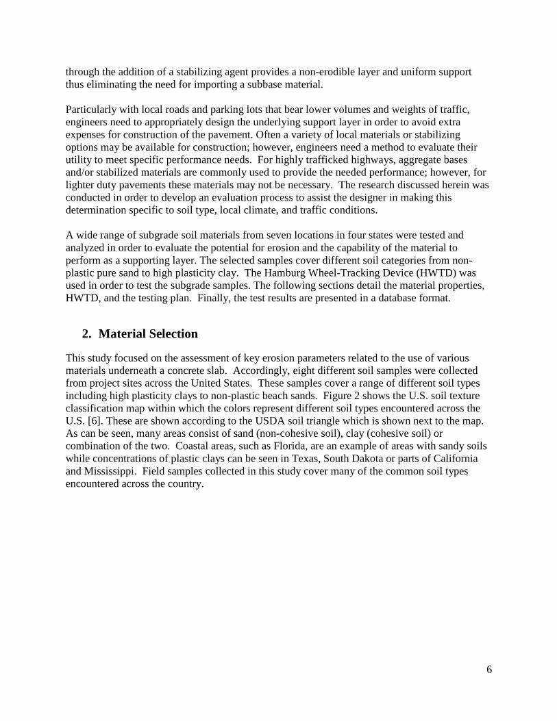
2. Material Selection

This study focused on the assessment of key erosion parameters related to the use of various materials underneath a concrete slab. Accordingly, eight different soil samples were collected from project sites across the United States. These samples cover a range of different soil types including high plasticity clays to non-plastic beach sands. Figure 2 shows the U.S. soil texture classification map within which the colors represent different soil types encountered across the U.S. [6]. These are shown according to the USDA soil triangle which is shown next to the map. As can be seen, many areas consist of sand (non-cohesive soil), clay (cohesive soil) or combination of the two. Coastal areas, such as Florida, are an example of areas with sandy soils while concentrations of plastic clays can be seen in Texas, South Dakota or parts of California and Mississippi. Field samples collected in this study cover many of the common soil types encountered across the country.

7

Figure 2 The Soil Classification Triangle and U.S. Soil Texture Classification Map [6].

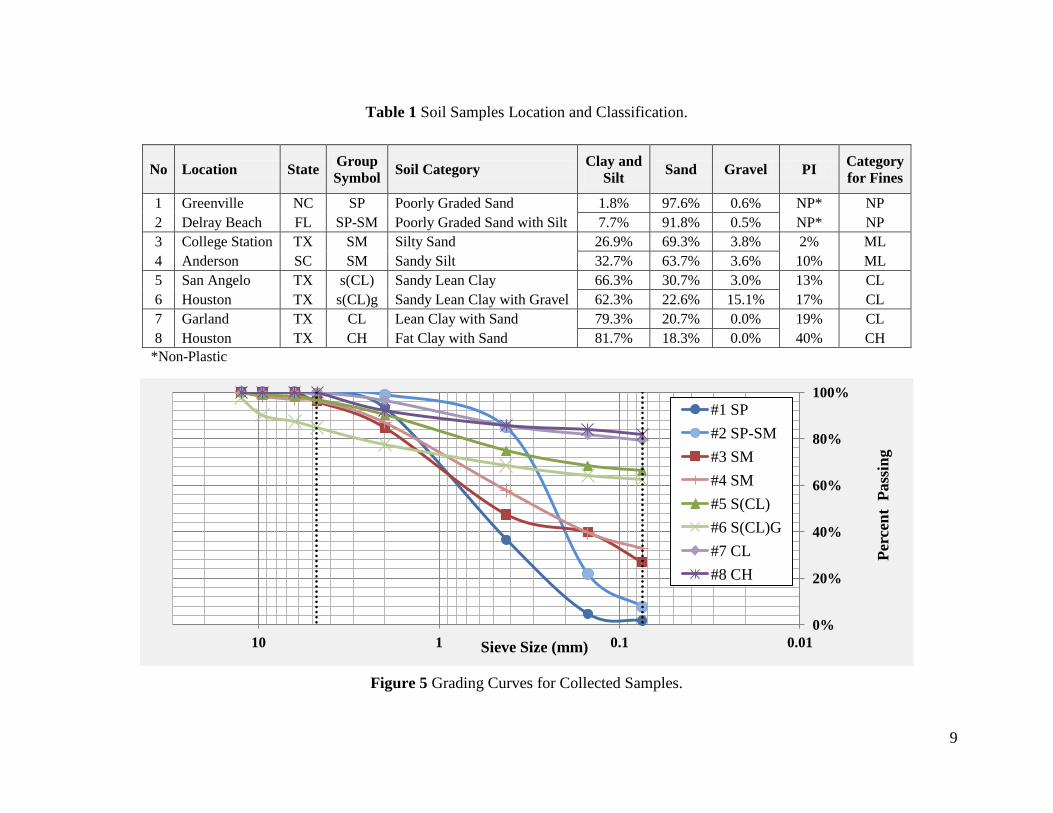
2.1 Gradation and Classification Dry and wet sieve analyses were performed on field soil samples to provide grading curves (ASTM D6913). Atterberg limits (liquid limit, plastic limit, and the plasticity index) on the fine portion of soils were determined (ASTM D4318). Soils were then classified according to the unified soil classification system (ASTM D2487) [7] [8] [9]. Results for the sieve analyses, grading curve, and Atterberg limits for each sample are shown in Appendix A and Appendix B. Table 1 summarizes the eight sample gradations and classifications. Sand is defined as particles of soil that pass a No. 4 (4.75 mm) sieve but are retained on the No. 200 (75 μm) sieve. Particles retrained on the No. 4 sieve (greater than 4.75 mm) are defined as gravel. Silt and clay are defined as particles that are smaller than 75 μm.[9]. Table 1 lists the samples in the order of increasing clay content and plasticity index. The soil samples were divided into four subcategories. The first two samples were considered to be pure sands with them being more than 90% of sand and non-cohesive. The sand from Florida (sample number two) is finer compared to the sand from North Carolina (sample number one). The second set of samples were sandy but contained silt. While the two samples in this set have similar grading, the plasticity index was significantly different between the two, with the sandy silt from South Carolina having a higher plasticity index than the silty sand from Texas. The third set was a combination of clay and sandy soils. The one from Houston (sample number six) had a higher plasticity index compared to the one from San Angelo (sample number five). And finally the last two samples were clays with plasticity indexes of 20% and 40%, while containing almost 80% or more of minus 200 sieve-sized particles. Figure 3 shows a comparison, distribution-wise, between a poorly graded sand and a fat clay demonstrating the significant differences in particle size. Figure 5 shows grading curves for the collected samples. Vertical dotted lines show the border between gravel-sand and sand-fine particles.

8

Figure 3 Comparison Between Two of the Sample’s Gradation.

Figure 4 shows the plasticity indices, PI, and percent minus #200 sieve of the collected samples. As mentioned before, samples are listed in the order of increasing clay content, as well as the plasticity index. These figures demonstrate that these samples represent common soil and base types found in the United States and used as sublayers for construction of concrete pavements.

Figure 4 PI for Each Sample Along with the Percent of Minus 200 (Silt and Clay).

1.8%

97.6%

0.6%

Poorly Graded Sand

% Fines

Sand

Gravel 81.7%

18.3% 0.0%

Fat Clay with Sand

Fines

Sand

Gravel

0%

20%

40%

60%

80%

100%

No.

1- S

P

No.

2- S

P-SM

No.

3- S

M

No.

4- S

M

No.

5- S

(CL

)

No.

6- S

(CL

)G

No.

7- C

L

No.

8- C

H

PI % Minus # 200 (Silt and Clay)

9

Table 1 Soil Samples Location and Classification.

No Location State Group Symbol Soil Category Clay and

Silt Sand Gravel PI Category for Fines

1 Greenville NC SP Poorly Graded Sand 1.8% 97.6% 0.6% NP* NP 2 Delray Beach FL SP-SM Poorly Graded Sand with Silt 7.7% 91.8% 0.5% NP* NP 3 College Station TX SM Silty Sand 26.9% 69.3% 3.8% 2% ML 4 Anderson SC SM Sandy Silt 32.7% 63.7% 3.6% 10% ML 5 San Angelo TX s(CL) Sandy Lean Clay 66.3% 30.7% 3.0% 13% CL 6 Houston TX s(CL)g Sandy Lean Clay with Gravel 62.3% 22.6% 15.1% 17% CL 7 Garland TX CL Lean Clay with Sand 79.3% 20.7% 0.0% 19% CL 8 Houston TX CH Fat Clay with Sand 81.7% 18.3% 0.0% 40% CH

*Non-Plastic

Figure 5 Grading Curves for Collected Samples.

0%

20%

40%

60%

80%

100%

0.01 0.1 1 10

Perc

ent

Pass

ing

Sieve Size (mm)

#1 SP #2 SP-SM #3 SM #4 SM #5 S(CL) #6 S(CL)G #7 CL #8 CH

10

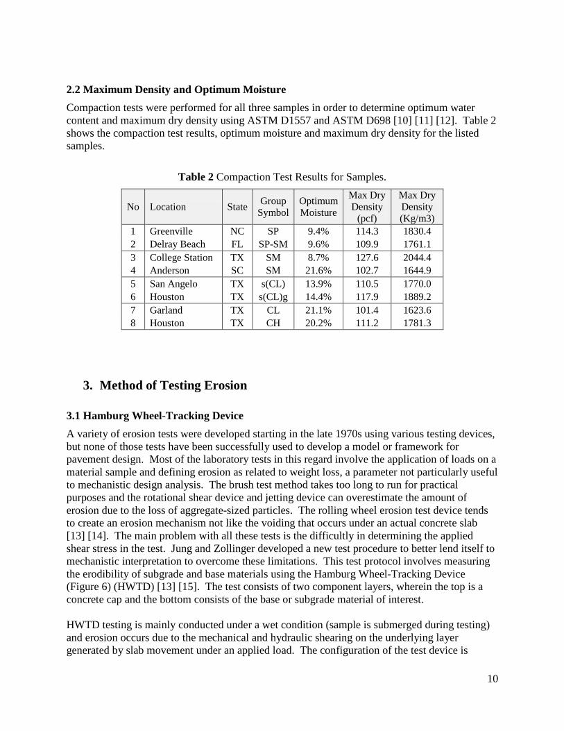
2.2 Maximum Density and Optimum Moisture Compaction tests were performed for all three samples in order to determine optimum water content and maximum dry density using ASTM D1557 and ASTM D698 [10] [11] [12]. Table 2 shows the compaction test results, optimum moisture and maximum dry density for the listed samples.

Table 2 Compaction Test Results for Samples.

No Location State Group Symbol

Optimum Moisture

Max Dry Density

(pcf)

Max Dry Density (Kg/m3)

1 Greenville NC SP 9.4% 114.3 1830.4 2 Delray Beach FL SP-SM 9.6% 109.9 1761.1 3 College Station TX SM 8.7% 127.6 2044.4 4 Anderson SC SM 21.6% 102.7 1644.9 5 San Angelo TX s(CL) 13.9% 110.5 1770.0 6 Houston TX s(CL)g 14.4% 117.9 1889.2 7 Garland TX CL 21.1% 101.4 1623.6 8 Houston TX CH 20.2% 111.2 1781.3

3. Method of Testing Erosion

3.1 Hamburg Wheel-Tracking Device A variety of erosion tests were developed starting in the late 1970s using various testing devices, but none of those tests have been successfully used to develop a model or framework for pavement design. Most of the laboratory tests in this regard involve the application of loads on a material sample and defining erosion as related to weight loss, a parameter not particularly useful to mechanistic design analysis. The brush test method takes too long to run for practical purposes and the rotational shear device and jetting device can overestimate the amount of erosion due to the loss of aggregate-sized particles. The rolling wheel erosion test device tends to create an erosion mechanism not like the voiding that occurs under an actual concrete slab [13] [14]. The main problem with all these tests is the difficultly in determining the applied shear stress in the test. Jung and Zollinger developed a new test procedure to better lend itself to mechanistic interpretation to overcome these limitations. This test protocol involves measuring the erodibility of subgrade and base materials using the Hamburg Wheel-Tracking Device (Figure 6) (HWTD) [13] [15]. The test consists of two component layers, wherein the top is a concrete cap and the bottom consists of the base or subgrade material of interest. HWTD testing is mainly conducted under a wet condition (sample is submerged during testing) and erosion occurs due to the mechanical and hydraulic shearing on the underlying layer generated by slab movement under an applied load. The configuration of the test device is

11

shown in Figure 6. The test configuration consists of a subgrade or base material, 154 mm (6 in.) in diameter and 25.4 mm (1 in.) thick, placed between a neoprene material (below) and a 25.4 mm (1 in.) thick jointed concrete block (above). The joint is sealed to simulate a joint in field conditions. A laboratory-compacted specimen or a core obtained from the field may be tested in the device. A wheel load of 71.6 kg (158 lb) is applied at a load frequency of 60-rpm. The depth of erosion at 11 locations is measured and then plotted versus the number of wheel load passes to graphically represent the erosion occurring in the base or soil sample [16] [5]. Erosion of the sublayer material is a result of the wheel load deflecting the concrete cap into the sublayer which induces shear stress and increased pore water pressure at the slab/sublayer interface. The HWTD is run until the point of failure in the sublayer.

Figure 6 Hamburg Wheel – Tracking Device (HWTD) [16].

3.2 Test Plan Since soil properties may change significantly due to changing moisture contents, some concern exists in regard to changes in a soil’s resistance against erosion. Water plays a significant role in the erosion process, particularly when the subgrade or base materials are saturated. Cohesive soils, like clays, are more sensitive to moisture content but since they contain higher portions of fine particles, it may take longer for water to fully saturate them. The test plan for erosion testing was designed to address various moisture contents experienced by base and subgrade materials with boundary conditions ranging from completely dry to fully saturated conditions. As previously explained, the HWTD contains a tank where the sample is placed and subjected to a passing wheel load. Under the wet condition, the tank is filled with water immediately prior to

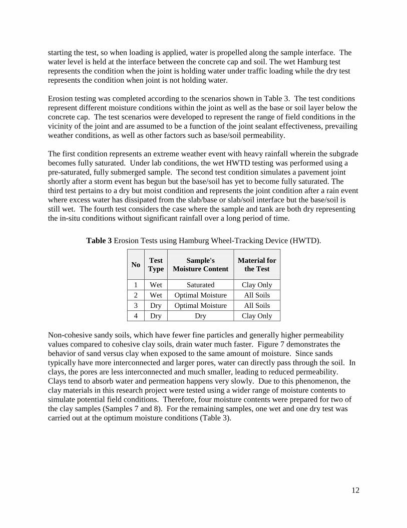
12

starting the test, so when loading is applied, water is propelled along the sample interface. The water level is held at the interface between the concrete cap and soil. The wet Hamburg test represents the condition when the joint is holding water under traffic loading while the dry test represents the condition when joint is not holding water. Erosion testing was completed according to the scenarios shown in Table 3. The test conditions represent different moisture conditions within the joint as well as the base or soil layer below the concrete cap. The test scenarios were developed to represent the range of field conditions in the vicinity of the joint and are assumed to be a function of the joint sealant effectiveness, prevailing weather conditions, as well as other factors such as base/soil permeability. The first condition represents an extreme weather event with heavy rainfall wherein the subgrade becomes fully saturated. Under lab conditions, the wet HWTD testing was performed using a pre-saturated, fully submerged sample. The second test condition simulates a pavement joint shortly after a storm event has begun but the base/soil has yet to become fully saturated. The third test pertains to a dry but moist condition and represents the joint condition after a rain event where excess water has dissipated from the slab/base or slab/soil interface but the base/soil is still wet. The fourth test considers the case where the sample and tank are both dry representing the in-situ conditions without significant rainfall over a long period of time.

Table 3 Erosion Tests using Hamburg Wheel-Tracking Device (HWTD).

No Test Type

Sample's Moisture Content

Material for the Test

1 Wet Saturated Clay Only 2 Wet Optimal Moisture All Soils 3 Dry Optimal Moisture All Soils 4 Dry Dry Clay Only

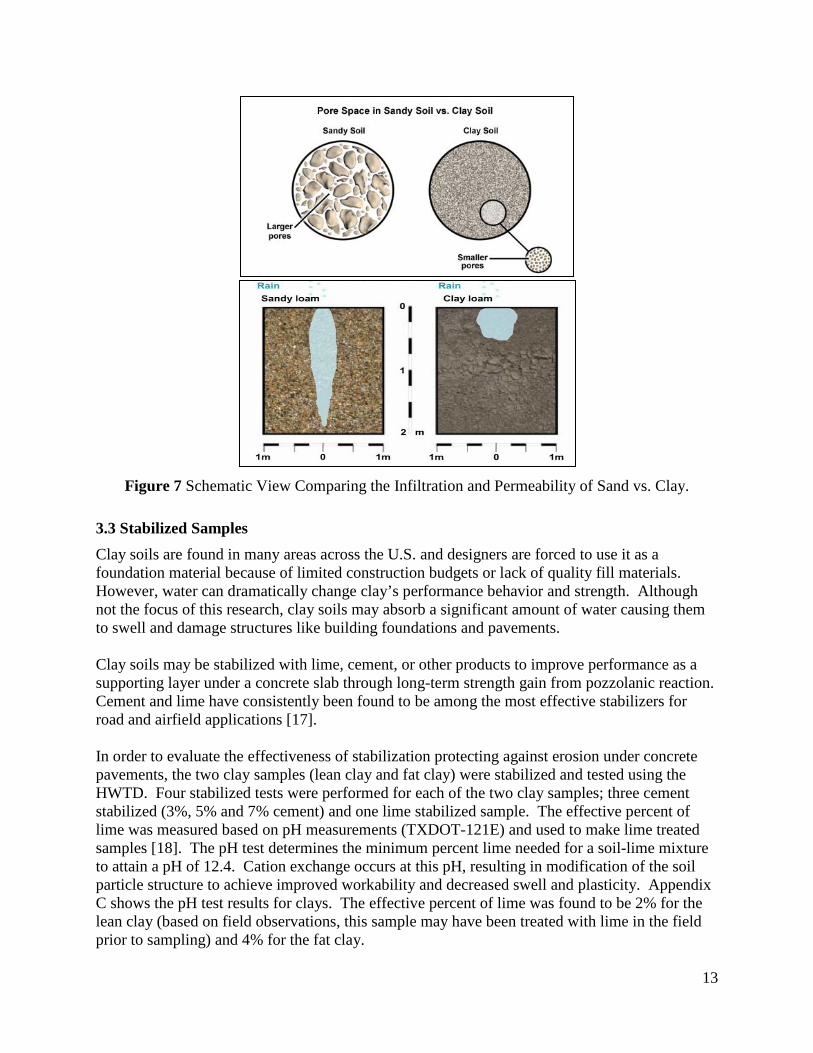
Non-cohesive sandy soils, which have fewer fine particles and generally higher permeability values compared to cohesive clay soils, drain water much faster. Figure 7 demonstrates the behavior of sand versus clay when exposed to the same amount of moisture. Since sands typically have more interconnected and larger pores, water can directly pass through the soil. In clays, the pores are less interconnected and much smaller, leading to reduced permeability. Clays tend to absorb water and permeation happens very slowly. Due to this phenomenon, the clay materials in this research project were tested using a wider range of moisture contents to simulate potential field conditions. Therefore, four moisture contents were prepared for two of the clay samples (Samples 7 and 8). For the remaining samples, one wet and one dry test was carried out at the optimum moisture conditions (Table 3).

13

Figure 7 Schematic View Comparing the Infiltration and Permeability of Sand vs. Clay.

3.3 Stabilized Samples Clay soils are found in many areas across the U.S. and designers are forced to use it as a foundation material because of limited construction budgets or lack of quality fill materials. However, water can dramatically change clay’s performance behavior and strength. Although not the focus of this research, clay soils may absorb a significant amount of water causing them to swell and damage structures like building foundations and pavements. Clay soils may be stabilized with lime, cement, or other products to improve performance as a supporting layer under a concrete slab through long-term strength gain from pozzolanic reaction. Cement and lime have consistently been found to be among the most effective stabilizers for road and airfield applications [17]. In order to evaluate the effectiveness of stabilization protecting against erosion under concrete pavements, the two clay samples (lean clay and fat clay) were stabilized and tested using the HWTD. Four stabilized tests were performed for each of the two clay samples; three cement stabilized (3%, 5% and 7% cement) and one lime stabilized sample. The effective percent of lime was measured based on pH measurements (TXDOT-121E) and used to make lime treated samples [18]. The pH test determines the minimum percent lime needed for a soil-lime mixture to attain a pH of 12.4. Cation exchange occurs at this pH, resulting in modification of the soil particle structure to achieve improved workability and decreased swell and plasticity. Appendix C shows the pH test results for clays. The effective percent of lime was found to be 2% for the lean clay (based on field observations, this sample may have been treated with lime in the field prior to sampling) and 4% for the fat clay.

14

Also, in order to test how sand’s behavior changes after stabilization, one of the sand samples was stabilized and tested under wet conditions using the HWTD.

4. Test Results

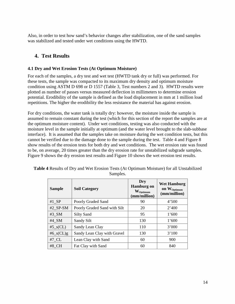
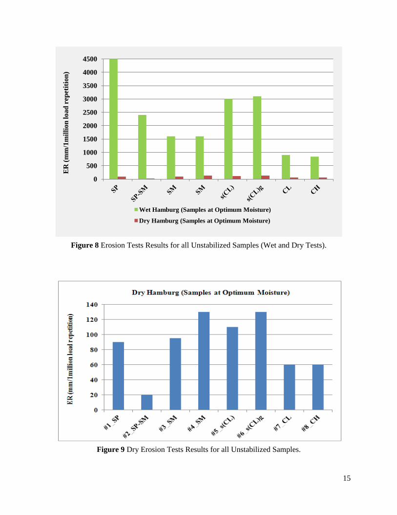
4.1 Dry and Wet Erosion Tests (At Optimum Moisture) For each of the samples, a dry test and wet test (HWTD tank dry or full) was performed. For these tests, the sample was compacted to its maximum dry density and optimum moisture condition using ASTM D 698 or D 1557 (Table 3, Test numbers 2 and 3). HWTD results were plotted as number of passes versus measured deflection in millimeters to determine erosion potential. Erodibility of the sample is defined as the load displacement in mm at 1 million load repetitions. The higher the erodibility the less resistance the material has against erosion. For dry conditions, the water tank is totally dry: however, the moisture inside the sample is assumed to remain constant during the test (which for this section of the report the samples are at the optimum moisture content). Under wet conditions, testing was also conducted with the moisture level in the sample initially at optimum (and the water level brought to the slab-subbase interface). It is assumed that the samples take on moisture during the wet condition tests, but this cannot be verified due to the damage done to the sample during the test. Table 4 and Figure 8 show results of the erosion tests for both dry and wet conditions. The wet erosion rate was found to be, on average, 20 times greater than the dry erosion rate for unstabilized subgrade samples. Figure 9 shows the dry erosion test results and Figure 10 shows the wet erosion test results.

Table 4 Results of Dry and Wet Erosion Tests (At Optimum Moisture) for all Unstabilized Samples.

Sample Soil Category

Dry Hamburg on

WOptimum (mm/million)

Wet Hamburg on WOptimum

(mm/million)

#1_SP Poorly Graded Sand 90 4’500 #2_SP-SM Poorly Graded Sand with Silt 20 2’400 #3_SM Silty Sand 95 1’600 #4_SM Sandy Silt 130 1’600 #5_s(CL) Sandy Lean Clay 110 3’000 #6_s(CL)g Sandy Lean Clay with Gravel 130 3’100 #7_CL Lean Clay with Sand 60 900 #8_CH Fat Clay with Sand 60 840

15

Figure 8 Erosion Tests Results for all Unstabilized Samples (Wet and Dry Tests).

Figure 9 Dry Erosion Tests Results for all Unstabilized Samples.

0

500

1000

1500

2000

2500

3000

3500

4000

4500 E

R (m

m/1

mill

ion

load

rep

etiti

on)

Wet Hamburg (Samples at Optimum Moisture)

Dry Hamburg (Samples at Optimum Moisture)

16

Figure 10 Wet Erosion Tests Results for all Unstabilized Samples.

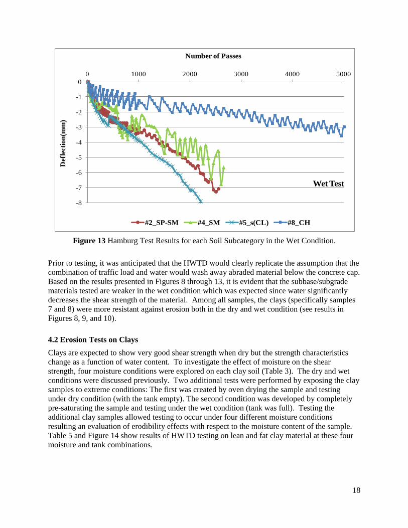
As previously discussed, samples were prepared from four subcategories of soils: sand, combination of silt and sand, combination of sand and clay, and clayey soils. Except for the sand, each of the materials from the other subcategories performed nearly the same under the wet and dry test conditions. As expected, the subgrade materials show relatively low erodibility in the dry condition and a high rate of erosion in the wet condition. Figure 11 shows the results of Hamburg tests for both the wet and dry samples from each subcategory. Individual results from each soil category under dry and wet conditions are shown on Figures 12 and 13, respectively. Appendix D includes graphs of all erosion test results collected for each sample.

17

Figure 11 Hamburg Test Results for each Subcategory Sample in both the Wet and Dry

Condition.

Figure 12 Hamburg Test Results for Each Soil Subcategory in the Dry Condition.

-8

-7

-6

-5

-4

-3

-2

-1

0 0 1000 2000 3000 4000 5000

Def

lect

ion(

mm

) Number of Passes

#2_SP-SM (Wet) #4_SM (Wet) #5_s(CL) (Wet) #8_CH (Wet) #2_SP-SM (Dry) #4_SM (Dry) #5_s(CL) (Dry) #8_CH (Dry)

-4.0

-3.5

-3.0

-2.5

-2.0

-1.5

-1.0

-0.5

0.00 1000 2000 3000 4000 5000

Def

lect

ion(

mm

)

Number of Passes

Dry Test

#2_SP-SM #4_SM #5_s(CL) #8_CH

18

Figure 13 Hamburg Test Results for each Soil Subcategory in the Wet Condition.

Prior to testing, it was anticipated that the HWTD would clearly replicate the assumption that the combination of traffic load and water would wash away abraded material below the concrete cap. Based on the results presented in Figures 8 through 13, it is evident that the subbase/subgrade materials tested are weaker in the wet condition which was expected since water significantly decreases the shear strength of the material. Among all samples, the clays (specifically samples 7 and 8) were more resistant against erosion both in the dry and wet condition (see results in Figures 8, 9, and 10).

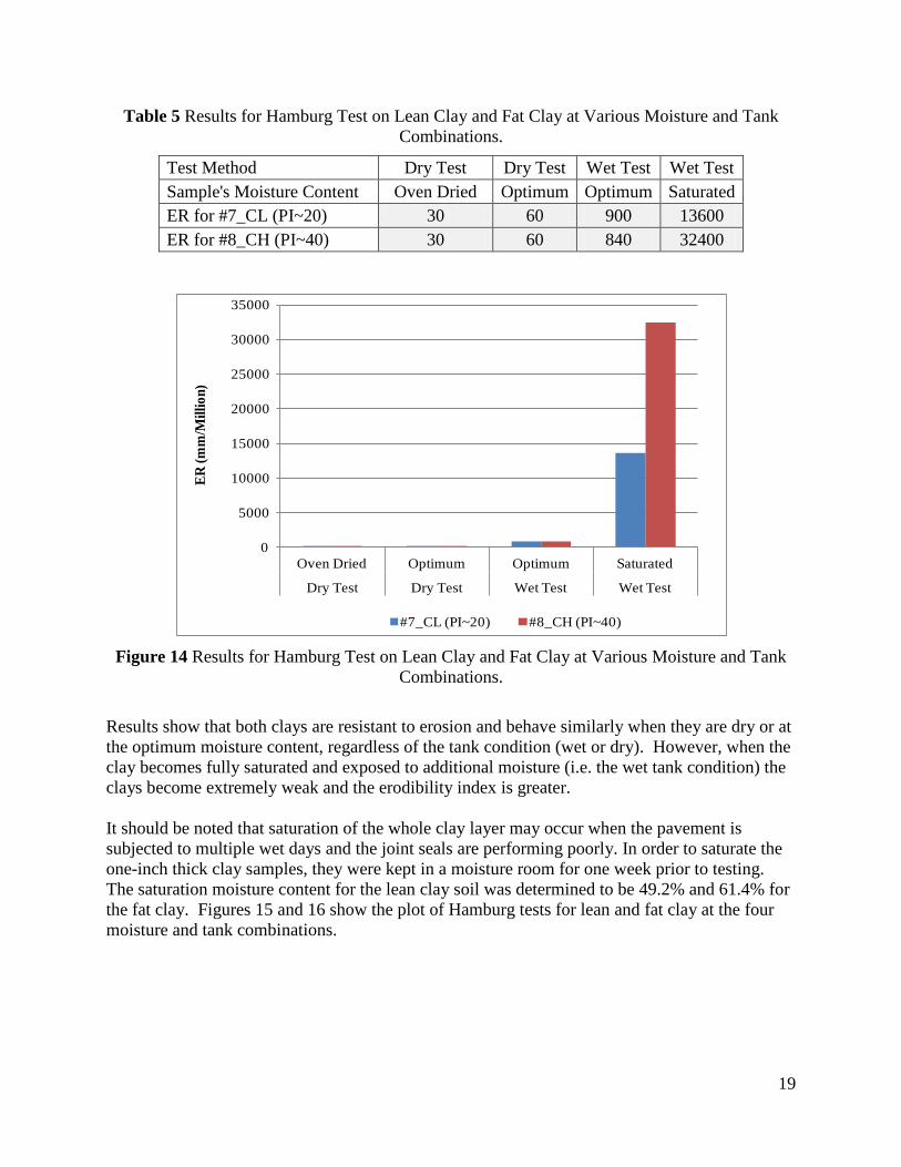
4.2 Erosion Tests on Clays Clays are expected to show very good shear strength when dry but the strength characteristics change as a function of water content. To investigate the effect of moisture on the shear strength, four moisture conditions were explored on each clay soil (Table 3). The dry and wet conditions were discussed previously. Two additional tests were performed by exposing the clay samples to extreme conditions: The first was created by oven drying the sample and testing under dry condition (with the tank empty). The second condition was developed by completely pre-saturating the sample and testing under the wet condition (tank was full). Testing the additional clay samples allowed testing to occur under four different moisture conditions resulting an evaluation of erodibility effects with respect to the moisture content of the sample. Table 5 and Figure 14 show results of HWTD testing on lean and fat clay material at these four moisture and tank combinations.

-8

-7

-6

-5

-4

-3

-2

-1

00 1000 2000 3000 4000 5000

Def

lectio

n(m

m)

Number of Passes

Wet Test

#2_SP-SM #4_SM #5_s(CL) #8_CH

19

Table 5 Results for Hamburg Test on Lean Clay and Fat Clay at Various Moisture and Tank Combinations.

Test Method Dry Test Dry Test Wet Test Wet Test Sample's Moisture Content Oven Dried Optimum Optimum Saturated ER for #7_CL (PI~20) 30 60 900 13600 ER for #8_CH (PI~40) 30 60 840 32400

Figure 14 Results for Hamburg Test on Lean Clay and Fat Clay at Various Moisture and Tank

Combinations. Results show that both clays are resistant to erosion and behave similarly when they are dry or at the optimum moisture content, regardless of the tank condition (wet or dry). However, when the clay becomes fully saturated and exposed to additional moisture (i.e. the wet tank condition) the clays become extremely weak and the erodibility index is greater. It should be noted that saturation of the whole clay layer may occur when the pavement is subjected to multiple wet days and the joint seals are performing poorly. In order to saturate the one-inch thick clay samples, they were kept in a moisture room for one week prior to testing. The saturation moisture content for the lean clay soil was determined to be 49.2% and 61.4% for the fat clay. Figures 15 and 16 show the plot of Hamburg tests for lean and fat clay at the four moisture and tank combinations.

0

5000

10000

15000

20000

25000

30000

35000

Oven Dried Optimum Optimum Saturated

Dry Test Dry Test Wet Test Wet Test

ER (m

m/M

illio

n)

#7_CL (PI~20) #8_CH (PI~40)

20

Figure 15 Hamburg Tests for Lean Clay, Sample Number 7.

Figure 16 Hamburg Tests for Fat Clay, Sample Number 8.

-9

-8

-7

-6

-5

-4

-3

-2

-1

00 500 1000 1500 2000 2500 3000 3500 4000 4500 5000

Def

lect

ion

(mm

)

Number of Passes

Oven Dry -Dry Test Saturated Wet TestOpt Moisture -Dry Test Opt Moisture -Wet Test

-9

-8

-7

-6

-5

-4

-3

-2

-1

00 500 1000 1500 2000 2500 3000 3500 4000 4500 5000

Def

lect

ion

(mm

)

Number of Passes

Oven Dry -Dry Test Saturated Wet Test

Opt Moisture -Dry Test Opt Moisture -Wet Test

21

4.3 Stabilized Clay Samples In order to evaluate the effectiveness of soil stabilization on erosion potential, four stabilized conditions were tested for the two clay samples described above. Three stabilization conditions were developed using cement at contents of 3%, 5% and 7%. One additional sample for each clay sample was prepared with lime. Samples were cured for 28 days and tested immediately after removal from the moisture room. The samples were also tested in the saturated condition because it was assumed that the erosion rate would have been minimal if tested dry or at optimum moisture. Effective percent of added lime was measured based on pH measurements following the Tex-121E test method [18]. The effective percent of lime was found to be 2% for the lean clay (based on field observations, this sample may have been treated with lime in the field prior to sampling) and 4% for the fat clay (see Appendix C for results from Tex-121-E). Table 6 and Figure 17 show results from HWTD testing on the stabilized clay samples. Figures 18 and 19 show the plot of HWTD testing for stabilized lean clay and fat clay samples.

Table 6 Results for Hamburg Test on Stabilized Clays.

Test Method Wet Test in Saturation

Wet Test in Saturation




% Stabilized 0% Cement 3% Cement 5% Cement 7% Cement Effective % of Lime

ER for #7_CL (PI~20) 13600 6400 3500 1100 3400 ER for #8_CH (PI~40) 32400 8200 5300 2200 4200

Figure 17 Results for Hamburg Test on Stabilized Clays.

0

5000

10000

15000

20000

25000

30000

35000

0% 3% 5% 7% Effective % of Lime

ER

(mm

/Mill

ion)

% Cement Stabilized #7_CL (PI~20) #8_CH (PI~40)

22

Figure 18 Hamburg Tests for Stabilized Lean Clay, Sample Number 7.

Figure 19 Hamburg Tests for Stabilized Fat Clay, Sample Number 8.

-9

-8

-7

-6

-5

-4

-3

-2

-1

00 200 400 600 800 1000 1200 1400

Def

lect

ion

(mm

)Number of Passes

Clay Garland Saturated Clay Garland 2% Lime Clay Garland 3% CementClay Garland 5% Cement Clay Garland 7% Cement

-6

-5

-4

-3

-2

-1

00 200 400 600 800 1000 1200 1400

Defle

ctio

n (m

m)

Number of Passes

Clay Houston Saturated Clay Houston 4% LimeClay Houston 3% Cement Clay Houston 5% CementClay Houston 7% Cement

23

As expected, stabilization significantly improved the resistance of the samples against erosion. Clays with less plasticity are shown to be stronger against erosion in the saturated condition when tested in the HWTD. Even though high plasticity clays have higher cohesiveness compared to low plastic clays, they absorbed more water when saturated; hence the reverse effect occurs because moisture weakens the high plasticity clay.

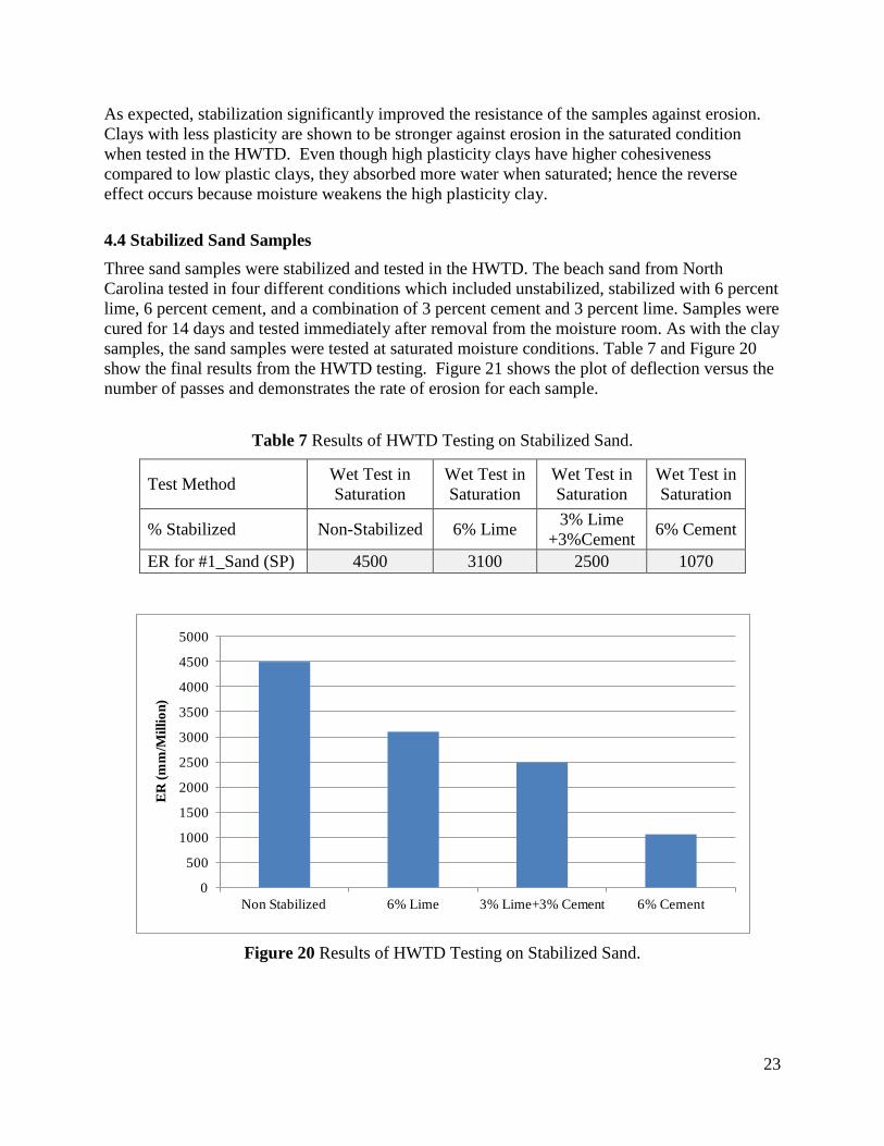
4.4 Stabilized Sand Samples Three sand samples were stabilized and tested in the HWTD. The beach sand from North Carolina tested in four different conditions which included unstabilized, stabilized with 6 percent lime, 6 percent cement, and a combination of 3 percent cement and 3 percent lime. Samples were cured for 14 days and tested immediately after removal from the moisture room. As with the clay samples, the sand samples were tested at saturated moisture conditions. Table 7 and Figure 20 show the final results from the HWTD testing. Figure 21 shows the plot of deflection versus the number of passes and demonstrates the rate of erosion for each sample.

Table 7 Results of HWTD Testing on Stabilized Sand.

Test Method Wet Test in Saturation




% Stabilized Non-Stabilized 6% Lime 3% Lime +3%Cement 6% Cement

ER for #1_Sand (SP) 4500 3100 2500 1070

Figure 20 Results of HWTD Testing on Stabilized Sand.

0

500

1000

1500

2000

2500

3000

3500

4000

4500

5000

Non Stabilized 6% Lime 3% Lime+3% Cement 6% Cement

ER

(mm

/Mill

ion)

24

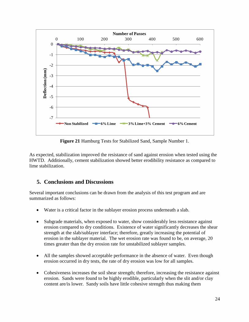
Figure 21 Hamburg Tests for Stabilized Sand, Sample Number 1.

As expected, stabilization improved the resistance of sand against erosion when tested using the HWTD. Additionally, cement stabilization showed better erodibility resistance as compared to lime stabilization.

5. Conclusions and Discussions

Several important conclusions can be drawn from the analysis of this test program and are summarized as follows:

• Water is a critical factor in the sublayer erosion process underneath a slab. • Subgrade materials, when exposed to water, show considerably less resistance against

erosion compared to dry conditions. Existence of water significantly decreases the shear strength at the slab/sublayer interface; therefore, greatly increasing the potential of erosion in the sublayer material. The wet erosion rate was found to be, on average, 20 times greater than the dry erosion rate for unstabilized sublayer samples.

• All the samples showed acceptable performance in the absence of water. Even though erosion occurred in dry tests, the rate of dry erosion was low for all samples.

• Cohesiveness increases the soil shear strength; therefore, increasing the resistance against erosion. Sands were found to be highly erodible, particularly when the slit and/or clay content are/is lower. Sandy soils have little cohesive strength thus making them

-7

-6

-5

-4

-3

-2

-1

00 100 200 300 400 500 600

Def

lect

ion

(mm

)

Number of Passes

Non Stabilized 6% Lime 3% Lime+3% Cement 6% Cement

25

susceptible to erosion. Clays, which typically have higher cohesiveness, on the other hand were found to be more resistant against erosion.

• While dried clays are very resistant against erosion, clays become extremely weak when

completely saturated. It should be noted that complete saturation of the whole clay layer rarely occurs unless a pavement system is in an extremely rainy climate with unsealed joints and poor drainage system.

• The results suggest that clays could be used as a suitable subgrade in a dry climate for minor roads or parking lots but using clays should be avoided in places with heavy rain and when unsealed joints may be used. Another potential problem with clays in changing moisture conditions is volume change that may cause damage to a concrete slab.

• Stabilization significantly improved the resistance of all samples against erosion. Seven

percent cement caused a decrease in erodibility index by 14 times in fat clays. Stabilization also improved the resistance of sand against erosion.

• Cement stabilization showed better erodibility resistance as compared to lime stabilization. Also, stabilization has greater impact on clay as compared to sands mainly because of faster and stronger chemical reactions of clay particles.

26

References

1. Selezneva, O., J. Jiang, and S.D. Tayabji, Preliminary Evaluation And Analysis Of LTPP Faulting Data-Final Report, 2000.

2. Neshvadian Bakhsh, K., D.G. Zollinger, and Y.-S. Jung. Evaluation of Joint Sealant Effectiveness on Moisture Infiltration and Erosion Potential in Concrete Pavement. in Transportation Research Board 92nd Annual Meeting. 2013.

3. Jung, Y.S., D.G. Zollinger, and T.J. Freeman, Evaluation and Decision Strategies for the Routine Maintenance of Concrete Pavement. 2009.

4. Freeman, T.J. and D.G. Zollinger, Guidelines for Routine Maintenance of Concrete Pavement, 2008.

5. Zollinger, D.G., et al., Subbase and Subgrade Performance Investigation and Design Guidelines for Concrete Pavement, 2012.

6. "USDA/The COMET Program". [Web] 2012 [cited 2012 10 September ]; Basic Hydrologic Science Course, Runoff Processes,Section Four: Soil Properties].

7. ASTM D6913 – 04 in Standard Test Methods for Particle-Size Distribution (Gradation) of Soils Using Sieve Analysis2009, American society for testing and materials.

8. ASTM D4318 – 10, in Standard Test Methods for Liquid Limit, Plastic Limit, and Plasticity Index of Soils2010, American Society for Testing and Materials.

9. ASTM D2487 – 11, in Standard Practice for Classification of Soils for Engineering Purposes (Unified Soil Classification System)2011, American Society for Testing and Materials.

10. ASTM D698 – 07, in Standard Test Methods for Laboratory Compaction Characteristics of Soil Using Standard Effort (12 400 ft-lbf/ft3 (600 kN-m/m3))2007, American Society for Testing and Materials.

11. ASTM D1557 – 09, in Standard Test Methods for Laboratory Compaction Characteristics of Soil Using Modified Effort (56,000 ft-lbf/ft3(2,700 kN-m/m3))2009, American Society for Testing and Materials.

12. ASTM D2216 – 10, in Standard Test Methods for Laboratory Determination of Water (Moisture) Content of Soil and Rock by Mass12010, American Society for Testing and Materials.

13. Jung, Y.S. and D.G. Zollinger, New Laboratory-Based Mechanistic-Empirical Model for Faulting in Jointed Concrete Pavement. Transportation Research Record: Journal of the Transportation Research Board, 2011. 2226(-1): p. 60-70.

14. De Beer, M., Aspects of Erodibility Lightly Cementitious Materials. South African Council for Scientific Industrial Research. . 1989: Flexible Pavement Programme.

15. TxDoT, Tex-242-F, in HAMBURG WHEEL-TRACKING TEST2009, Texas Department of Transportation.

27

16. Jung, Y.S., D.G. Zollinger, and A.J. Wimsatt, Test Method and Model Development of Subbase Erosion for Concrete Pavement Design. Transportation Research Record: Journal of the Transportation Research Board, 2010. 2154(-1): p. 22-31.

17. Kawamura, M. and S. Diamond, Stabilization of clay soils against erosion loss, 1975.

18. Tex-121-E, in SOIL-LIME TESTING2002, Texas Department of Transportation.

19. Sahin, H., F. Gu, and R.L. Lytton, Development of Soil Water Characteristic Curve for Flexible Base Materials Using the Methylene Blue Test. Transportation Research Record: Journal of the Transportation Research Board 2013. Under Press.

20. Lindeburg, M.R., Civil engineering reference manual for the PE exam. 2012: www. ppi2pass. com.

28

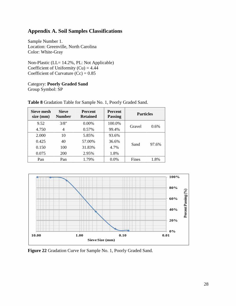
Appendix A. Soil Samples Classifications

Sample Number 1. Location: Greenville, North Carolina Color: White-Gray Non-Plastic (LL= 14.2%, PL: Not Applicable) Coefficient of Uniformity (Cu) = 4.44 Coefficient of Curvature (Cc) = 0.85 Category: Poorly Graded Sand Group Symbol: SP

Table 8 Gradation Table for Sample No. 1, Poorly Graded Sand.

Sieve mesh size (mm)

Sieve Number

Percent Retained

Percent Passing Particles

9.52 3/8" 0.00% 100.0% Gravel 0.6%

4.750 4 0.57% 99.4% 2.000 10 5.85% 93.6%

Sand 97.6% 0.425 40 57.00% 36.6% 0.150 100 31.83% 4.7% 0.075 200 2.95% 1.8% Pan Pan 1.79% 0.0% Fines 1.8%

Figure 22 Gradation Curve for Sample No. 1, Poorly Graded Sand.

0%

20%

40%

60%

80%

100%

0.010.101.0010.00

Perc

ent P

assin

g (%

)

Sieve Size (mm)

29

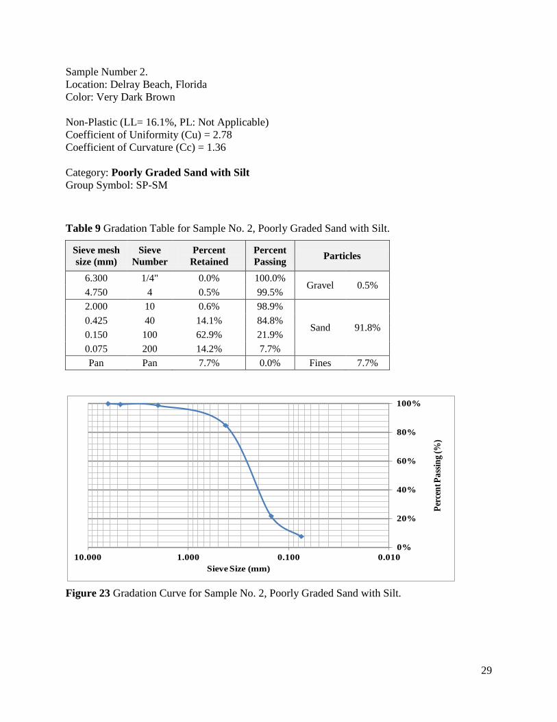
Sample Number 2. Location: Delray Beach, Florida Color: Very Dark Brown Non-Plastic (LL= 16.1%, PL: Not Applicable) Coefficient of Uniformity (Cu) = 2.78 Coefficient of Curvature (Cc) = 1.36 Category: Poorly Graded Sand with Silt Group Symbol: SP-SM

Table 9 Gradation Table for Sample No. 2, Poorly Graded Sand with Silt.


Sieve Number

Percent Retained


6.300 1/4" 0.0% 100.0% Gravel 0.5%

4.750 4 0.5% 99.5% 2.000 10 0.6% 98.9%


Figure 23 Gradation Curve for Sample No. 2, Poorly Graded Sand with Silt.

0%

20%

40%

60%

80%

100%

0.0100.1001.00010.000

Perc

ent P

assin

g (%

)

Sieve Size (mm)

30

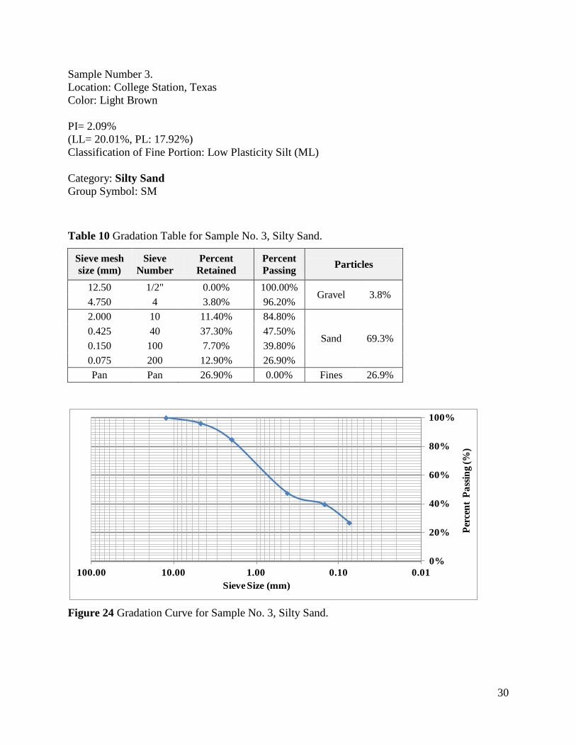
Sample Number 3. Location: College Station, Texas Color: Light Brown PI= 2.09% (LL= 20.01%, PL: 17.92%) Classification of Fine Portion: Low Plasticity Silt (ML) Category: Silty Sand Group Symbol: SM

Table 10 Gradation Table for Sample No. 3, Silty Sand.


Sieve Number

Percent Retained


12.50 1/2" 0.00% 100.00% Gravel 3.8%

4.750 4 3.80% 96.20% 2.000 10 11.40% 84.80%


Figure 24 Gradation Curve for Sample No. 3, Silty Sand.

0%

20%

40%

60%

80%

100%

0.010.101.0010.00100.00

Perc

ent

Pass

ing (

%)

Sieve Size (mm)

31

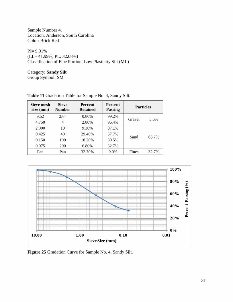
Sample Number 4. Location: Anderson, South Carolina Color: Brick Red PI= 9.91% (LL= 41.99%, PL: 32.08%) Classification of Fine Portion: Low Plasticity Silt (ML) Category: Sandy Silt Group Symbol: SM

Table 11 Gradation Table for Sample No. 4, Sandy Silt.


Sieve Number

Percent Retained


9.52 3/8" 0.80% 99.2% Gravel 3.6%

4.750 4 2.80% 96.4% 2.000 10 9.30% 87.1%


Figure 25 Gradation Curve for Sample No. 4, Sandy Silt.

0%

20%

40%

60%

80%

100%

0.010.101.0010.00

Perc

ent

Pass

ing (

%)

Sieve Size (mm)

32

Sample Number 5. Location: San Angelo, Texas Color: Dark Brown PI= 13.36% (LL= 32.36%, PL: 19.00%) Classification of Fine Portion: Low Plasticity Clay (CL) Category: Sandy Lean Clay Group Symbol: s(CL)

Table 12 Gradation Table for Sample No. 5, Sandy Lean Clay.


Sieve Number

Percent Retained


12.50 1/2" 0.0% 100.0% Gravel 3.0%

4.750 4 3.0% 97.0% 2.000 10 6.7% 90.3%


Figure 26 Gradation Curve for Sample No. 5, Sandy Lean Clay.

0%

20%

40%

60%

80%

100%

0.010.101.0010.00

Perc

ent P

assin

g (%

)

Sieve Size (mm)

33

Sample Number 6. Location: Houston, Texas Color: Brown PI= 17.34% (LL= 33.59%, PL: 16.25%) Classification of Fine Portion: Low Plasticity Clay (CL) Category: Sandy Lean Clay with Gravel Group Symbol: s(CL)g

Table 13 Gradation Table for Sample No. 6, Sandy Lean Clay with Gravel.


Sieve Number

Percent Retained


12.50 1/2" 2.5% 97.5% Gravel 15.1%

4.750 4 12.6% 84.9% 2.000 10 7.3% 77.6%


Figure 27 Gradation Curve for Sample No. 6, Sandy Lean Clay with Gravel.

0%

20%

40%

60%

80%

100%

0.010.101.0010.00

Perc

ent

Pass

ing (

%)

Sieve Size (mm)

34

Sample Number 7. Location: Garland, Texas Color: Grayish Brown PI= 19.17% (LL= 41.78%, PL: 22.61%) Classification of Fine Portion: Low Plasticity Clay (CL) Category: Lean Clay with Sand Group Symbol: CL

Table 14 Gradation Table for Sample No. 7, Lean Clay with Sand.


Sieve Number

Percent Retained


12.50 1/2" 0.00% 100.0% Gravel 0.0%

4.750 4 0.00% 100.0% 2.000 10 3.50% 96.5%


Figure 28 Gradation Curve for Sample No. 7, Lean Clay with Sand.

0%

20%

40%

60%

80%

100%

0.010.101.0010.00

Perc

ent

Pass

ing (

%)

Sieve Size (mm)

35

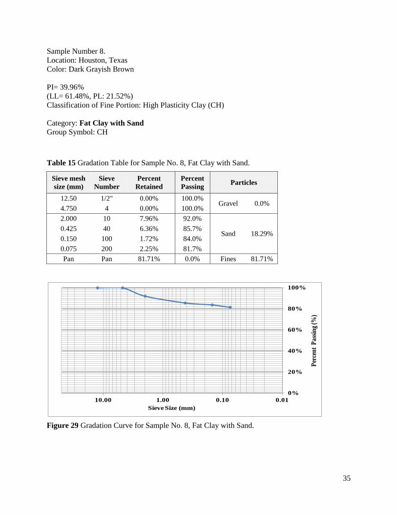
Sample Number 8. Location: Houston, Texas Color: Dark Grayish Brown PI= 39.96% (LL= 61.48%, PL: 21.52%) Classification of Fine Portion: High Plasticity Clay (CH) Category: Fat Clay with Sand Group Symbol: CH

Table 15 Gradation Table for Sample No. 8, Fat Clay with Sand.


Sieve Number

Percent Retained


12.50 1/2" 0.00% 100.0% Gravel 0.0%

4.750 4 0.00% 100.0% 2.000 10 7.96% 92.0%


Figure 29 Gradation Curve for Sample No. 8, Fat Clay with Sand.

0%

20%

40%

60%

80%

100%

0.010.101.0010.00

Perc

ent P

assin

g (%

)

Sieve Size (mm)

36

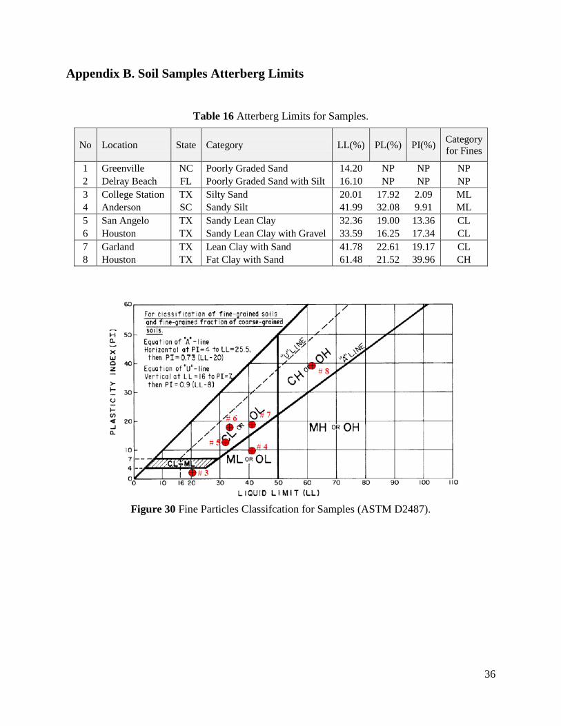
Appendix B. Soil Samples Atterberg Limits

Table 16 Atterberg Limits for Samples.

No Location State Category LL(%) PL(%) PI(%) Category for Fines

1 Greenville NC Poorly Graded Sand 14.20 NP NP NP 2 Delray Beach FL Poorly Graded Sand with Silt 16.10 NP NP NP 3 College Station TX Silty Sand 20.01 17.92 2.09 ML 4 Anderson SC Sandy Silt 41.99 32.08 9.91 ML 5 San Angelo TX Sandy Lean Clay 32.36 19.00 13.36 CL 6 Houston TX Sandy Lean Clay with Gravel 33.59 16.25 17.34 CL 7 Garland TX Lean Clay with Sand 41.78 22.61 19.17 CL 8 Houston TX Fat Clay with Sand 61.48 21.52 39.96 CH

Figure 30 Fine Particles Classifcation for Samples (ASTM D2487).

37

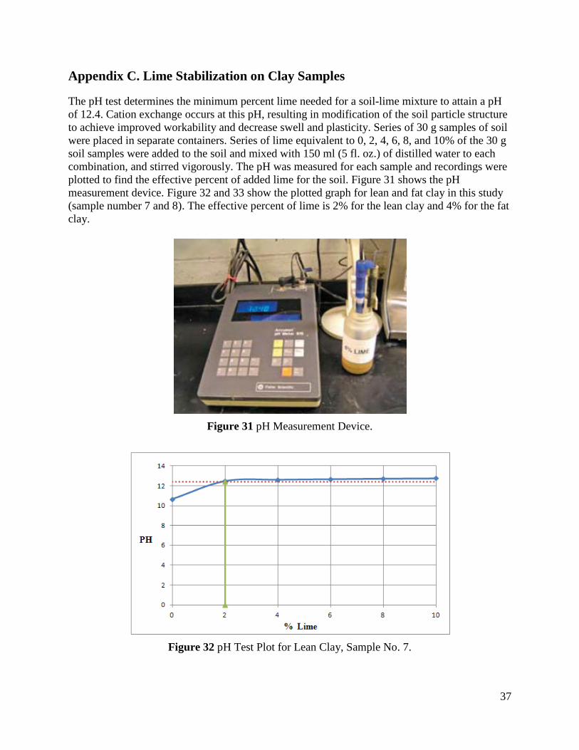
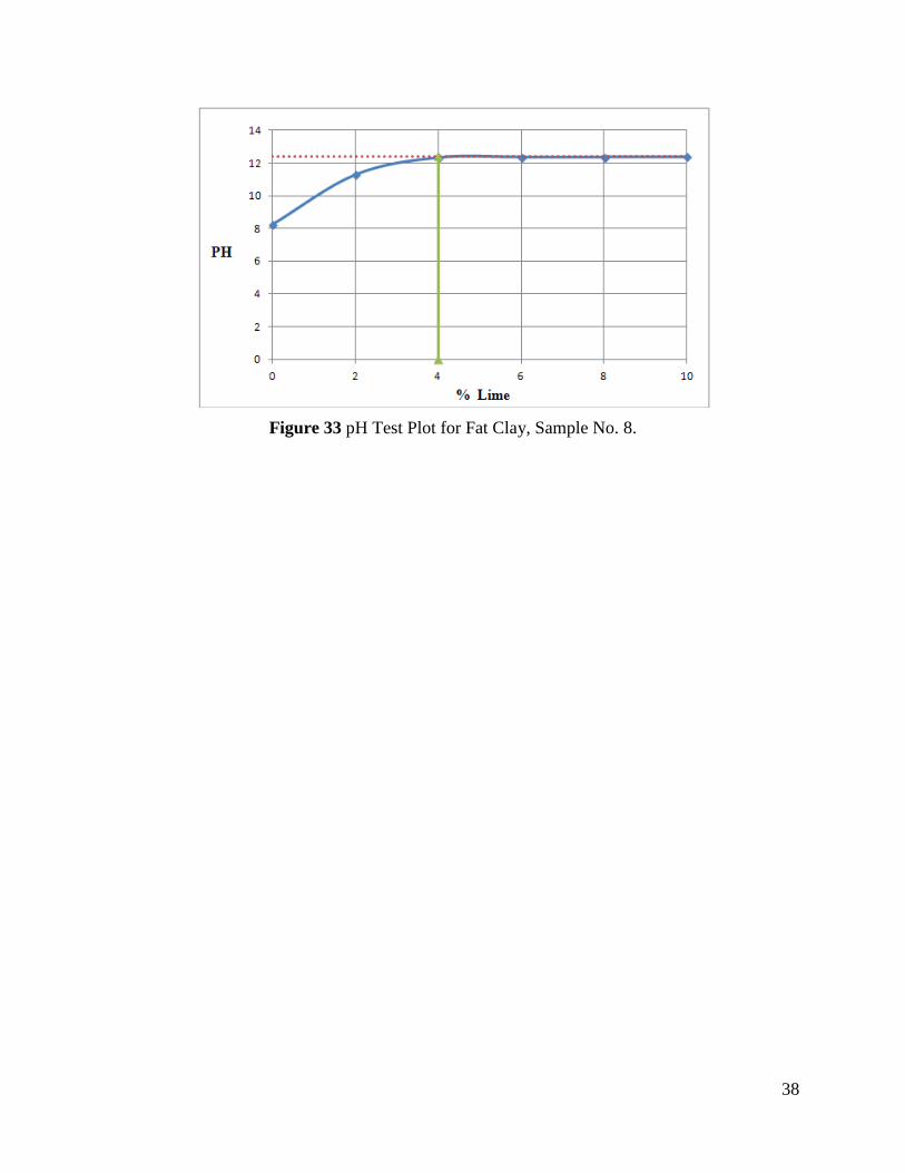
Appendix C. Lime Stabilization on Clay Samples

The pH test determines the minimum percent lime needed for a soil-lime mixture to attain a pH of 12.4. Cation exchange occurs at this pH, resulting in modification of the soil particle structure to achieve improved workability and decrease swell and plasticity. Series of 30 g samples of soil were placed in separate containers. Series of lime equivalent to 0, 2, 4, 6, 8, and 10% of the 30 g soil samples were added to the soil and mixed with 150 ml (5 fl. oz.) of distilled water to each combination, and stirred vigorously. The pH was measured for each sample and recordings were plotted to find the effective percent of added lime for the soil. Figure 31 shows the pH measurement device. Figure 32 and 33 show the plotted graph for lean and fat clay in this study (sample number 7 and 8). The effective percent of lime is 2% for the lean clay and 4% for the fat clay.

Figure 31 pH Measurement Device.

Figure 32 pH Test Plot for Lean Clay, Sample No. 7.

38

Figure 33 pH Test Plot for Fat Clay, Sample No. 8.

39

Appendix D. Hamburg Test Results

Erosion test results for each of the collected sample are shown in this Appendix.

Figure 34 Erosion Test Results for Poorly Graded Sand.

Figure 35 Erosion Test Results for Poorly Graded Sand with Silt.

-8 -7 -6 -5 -4 -3 -2 -1 0

0 1000 2000 3000 4000 5000

Def

lect

ion(

mm

)

Number of Passes

#1_SP(Wet) #1_SP(Dry)

-8 -7 -6 -5 -4 -3 -2 -1 0

0 1000 2000 3000 4000 5000

Def

lect

ion(

mm

)

Number of Passes

#2_SP-SM (Wet) #2_SP-SM (Dry)

40

Figure 36 Erosion Test Results for Silty Sand.

Figure 37 Erosion Test Results for Sandy Silt.

-8 -7 -6 -5 -4 -3 -2 -1 0

0 1000 2000 3000 4000 5000

Def

lect

ion(

mm

) Number of Passes

#3_SM (Wet) #3_SM (Dry)

-8 -7 -6 -5 -4 -3 -2 -1 0

0 1000 2000 3000 4000 5000

Def

lect

ion(

mm

)

Number of Passes

#4_SM (Wet) #4_SM (Dry)

41

Figure 38 Erosion Test Results for Sandy Lean Clay.

Figure 39 Erosion Test Results for Sandy Lean Clay with Gravel.

-8 -7 -6 -5 -4 -3 -2 -1 0

0 1000 2000 3000 4000 5000 D

efle

ctio

n(m

m)

Number of Passes

#5_s(CL) (Wet) #5_s(CL) (Dry)

-8 -7 -6 -5 -4 -3 -2 -1 0

0 1000 2000 3000 4000 5000

Def

lect

ion(

mm

)

Number of Passes

#6_s(CL)g (Wet) #6_s(CL)g (Dry)

42

Figure 40 Erosion Test Results for Lean Clay with Sand.

Figure 41 Erosion Test Results for Fat Clay with Sand.

-8 -7 -6 -5 -4 -3 -2 -1 0

0 1000 2000 3000 4000 5000 D

efle

ctio

n(m

m)

Number of Passes

#7_CL (Wet) #7_CL (Dry)

-8 -7 -6 -5 -4 -3 -2 -1 0

0 1000 2000 3000 4000 5000

Def

lect

ion(

mm

)

Number of Passes

#8_CH (Wet) #8_CH (Dry)

43

Appendix E. Suggested Test Procedure; Methylene Blue Test

In order to define the soil classification, another test method is suggested. The Methylene Blue Value (MBV) provides an indication of amount and activity of clay present in soil sample. The MBV is a new, rapid method for measuring Methylene Blue Value. In contrast to time consuming traditional tests, the Methylene Blue Test is quick and is completed in nearly 10 minutes. The apparatus is portable and the procedure is simple. The direct outcome of the MBV test is to define the percent of clay in the soil sample. That can be used to get Plasticity Index (PI), Liquid Limit (LL), and Cohesion value with an acceptable accuracy. Appendix E contains an explanation of MBV test. It also includes comparison of values gained by common test methods for one of the soil samples (sample number four) to the values gained by MBV method which shows the accuracy of the MBV test results.

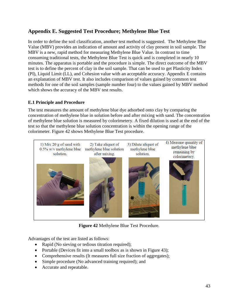
E.1 Principle and Procedure The test measures the amount of methylene blue dye adsorbed onto clay by comparing the concentration of methylene blue in solution before and after mixing with sand. The concentration of methylene blue solution is measured by colorimetery. A fixed dilution is used at the end of the test so that the methylene blue solution concentration is within the opening range of the colorimeter. Figure 42 shows Methylene Blue Test procedure.

Figure 42 Methylene Blue Test Procedure.

Advantages of the test are listed as follows:

• Rapid (No sieving or tedious titration required); • Portable (Devices fit into a small toolbox as is shown in Figure 43); • Comprehensive results (It measures full size fraction of aggregates); • Simple procedure (No advanced training required); and • Accurate and repeatable.

44

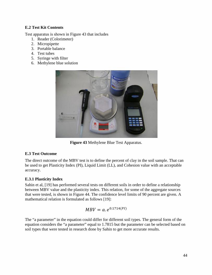
E.2 Test Kit Contents Test apparatus is shown in Figure 43 that includes

1. Reader (Colorimeter) 2. Micropipette 3. Portable balance 4. Test tubes 5. Syringe with filter 6. Methylene blue solution

Figure 43 Methylene Blue Test Apparatus.

E.3 Test Outcome The direct outcome of the MBV test is to define the percent of clay in the soil sample. That can be used to get Plasticity Index (PI), Liquid Limit (LL), and Cohesion value with an acceptable accuracy.

E.3.1 Plasticity Index Sahin et al, [19] has performed several tests on different soils in order to define a relationship between MBV value and the plasticity index. This relation, for some of the aggregate sources that were tested, is shown in Figure 44. The confidence level limits of 90 percent are given. A mathematical relation is formulated as follows [19]:

𝑀𝐵𝑉 = 𝑎. 𝑒0.1714(𝑃𝐼) The “a parameter” in the equation could differ for different soil types. The general form of the equation considers the “a parameter” equal to 1.7815 but the parameter can be selected based on soil types that were tested in research done by Sahin to get more accurate results.

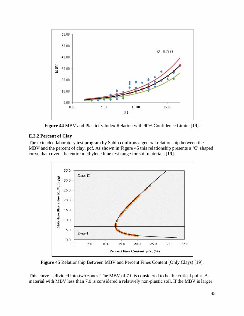
45

Figure 44 MBV and Plasticity Index Relation with 90% Confidence Limits [19].

E.3.2 Percent of Clay The extended laboratory test program by Sahin confirms a general relationship between the MBV and the percent of clay, pcf. As shown in Figure 45 this relationship presents a ‘C’ shaped curve that covers the entire methylene blue test range for soil materials [19].

Figure 45 Relationship Between MBV and Percent Fines Content (Only Clays) [19].

This curve is divided into two zones. The MBV of 7.0 is considered to be the critical point. A material with MBV less than 7.0 is considered a relatively non-plastic soil. If the MBV is larger

46

than 7.0 the material has high plasticity. A mathematical correlation model is determined between MBV and percent fines content. The model present quantitative amount of clay content as follows [19]:

𝑝𝑐𝑓 =27.601𝑀𝐵𝑉0.923 + 1.552 (𝑀𝐵𝑉)

Where MBV is the methylene blue value; pcf is the percent clay content. The coefficients are the general forms but there are tables based on soil types that help to get even more accurate values.

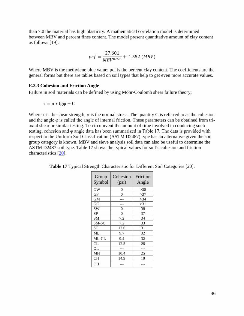
E.3.3 Cohesion and Friction Angle Failure in soil materials can be defined by using Mohr-Coulomb shear failure theory; τ = σ ∗ tgφ + C Where τ is the shear strength, σ is the normal stress. The quantity C is referred to as the cohesion and the angle φ is called the angle of internal friction. These parameters can be obtained from tri-axial shear or similar testing. To circumvent the amount of time involved in conducing such testing, cohesion and φ angle data has been summarized in Table 17. The data is provided with respect to the Uniform Soil Classification (ASTM D2487) type has an alternative given the soil group category is known. MBV and sieve analysis soil data can also be useful to determine the ASTM D2487 soil type. Table 17 shows the typical values for soil’s cohesion and friction characteristics [20].

Table 17 Typical Strength Characteristic for Different Soil Categories [20].

Group Symbol

Cohesion (psi)

Friction Angle

GW 0 >38 GP 0 >37 GM --- >34 GC --- >31 SW 0 38 SP 0 37 SM 7.2 34 SM-SC 7.2 33 SC 13.6 31 ML 9.7 32 ML-CL 9.4 32 CL 12.5 28 OL --- --- MH 10.4 25 CH 14.9 19 OH --- ---

47

E. 4 Test Validation with Lab Data In order to validate the MBV test and corresponding values, one of the soil samples was tested. The sandy silt from Anderson, South Carolina (Sample No.4) was tested and the MBV value for the sample is 6.44. Also, the hydrometric analysis was performed in order to find the percent of clay. The total percent of fines (clay and silt) was known from sieve analysis (32.07%). Horiba la-910 was used for hydrometric analysis. Horiba LA-910 is a laser scattering particle size analyzer. Hydrometric results are shown in Figure 46. Accordingly, 12.2% of the sample is clay (particle size smaller than 2 micro millimeters).

Figure 46 Hydrometric Results for South Carolina Sandy Silt.

Table 18 shows the test results on South Carolina sample using traditional test methods. Table 19 compares values calculated by traditional test methods versus the values using MBV value. It can be seen that errors are negligible and the MBV results are close to the common test results.

Table 18 Test Results on South Carolina Sample Using Traditional Test Methods.

Sample Location

Group Symbol Category Percent

of Fines Percent of Sand

Percent of

Gravel PI Percent

of Clay

Anderson, Sc SM Sandy Silt 32.7% 63.7% 3.6% 9.92% 12.20%

Table 19 Comparison of Values Gained By Common Methods Vs. Values Using MBV.

MBV PI % of Error pcf % of Error 6.44 9.52% 4.05% 11.72% 3.94%

https://www.google.com/url?sa=t&rct=j&q=&esrc=s&source=web&cd=6&cad=rja&ved=0CEoQFjAF&url=http%3A%2F%2Fmax.materials.drexel.edu%2Flab-facilities%2Fimg_0339%2F&ei=OhFGUq6FJMag2gXL_4HwCA&usg=AFQjCNGWeueLd9e93vlr1Jo5M6PqCeXvCw&sig2=n740xLmOE_bf0NmgQiDm8Q&bvm=bv.53217764,d.b2I

https://www.google.com/url?sa=t&rct=j&q=&esrc=s&source=web&cd=6&cad=rja&ved=0CEoQFjAF&url=http%3A%2F%2Fmax.materials.drexel.edu%2Flab-facilities%2Fimg_0339%2F&ei=OhFGUq6FJMag2gXL_4HwCA&usg=AFQjCNGWeueLd9e93vlr1Jo5M6PqCeXvCw&sig2=n740xLmOE_bf0NmgQiDm8Q&bvm=bv.53217764,d.b2I

test methods & results of erosion potential of commonly ... · test methods & results of...

Documents